SCHUMPETER DISCUSSION PAPERS Quiet please! Adverse...

SCHUMPETER DISCUSSION PAPERS

Quiet please! Adverse effects of noise on child development

Anna Makles and Kerstin Schneider

SDP 2016-002 ISSN 1867-5352

© by the author

1

Quiet please! Adverse effects of noise on child development

Anna Makles* - Kerstin Schneider+#

May 2016

Abstract

Noise pollution is detrimental to health and to cognitive development of children. This is not

only true for extreme levels of noise in the neighborhood of an airport but also to traffic noise

in urban areas. Using a census of preschool children, we show that children who are exposed

to intensive traffic noise significantly fall behind in terms of school readiness. Being exposed

to additional 10 dB(A) compares to about 3 months in kindergarten. We contribute to the lit-

erature and the policy debate by working with administrative data and focusing on everyday

exposure to noise. The proposed method is easily applied to other regions. We assess the pub-

lic costs of different abatement instruments and compare the costs to the benefits. It turns out

that the commonly used abatement measures like quiet pavement or noise protection walls in

densely populated areas of about 3,000 to 5,000 inhabitants per km2 can be cost efficient,

even with a conservative assessment of the benefits.

Keywords: Noise; child development; early education; abatement; abatement costs

JEL Classification: Q53; I18; I26; H23; H54

*Anna Makles, Wuppertal Research Institute for the Economics of Education (WIB), Univer-sity of Wuppertal, Gaußstr. 20, 42119 Wuppertal, [email protected], www.wib.uni-wuppertal.de +Kerstin Schneider, Wuppertal Research Institute for the Economics of Education (WIB), University of Wuppertal, Gaußstr. 20, 42119 Wuppertal, [email protected], www.wib.uni-wuppertal.de and CESifo #Corresponding Author: Phone: +49 (0)202 439 2483, Fax: +49 (0)202 439 3649

SCHUMPETER DISCUSSION PAPERS 2016-002

2

Introduction

Children are exposed to noise throughout the day and also at night. In kindergarten, for exam-

ple, the noise level produced by children themselves may even exceed 120 dB(A)1, which

corresponds to a jet take-off in 160 meters distance. And if the kindergarten is located at a

busy street, children are exposed to a permanent sound level of about 90 dB(A). This is louder

than a hairdryer and might cause severe and chronic hearing damage (Tamburlini 2002, p.

32). Back at home, TV noise, background music, the vacuum cleaner and toys produce intru-

sive or annoying sounds. A rubber duck causes the same sound pressure level as a diesel

truck; but, off course, no one is exposed to the sound of a rubber duck 24 hours a day. More

importantly, exposure to aircraft and traffic noise has become one of the biggest problems of

industrial countries and especially urban regions (WHO 2011).

The effect of environmental pollution on child development has been on the research

agenda with a focus on air pollution (for a survey cf. Currie et al. 2014, Coneus/Spiess 2012).

The effects of noise are less prominent in the economic literature, but have been studied in

many ways. Impairment of early childhood development caused by noise may have lifelong

effects on academic achievement and health. Especially indirect adverse effects of persistent

noise on children’s health and development are fairly well understood. There is evidence for

negative effects on child’s health through different channels, e.g. blood pressure, stress hor-

mones, sleep quality or mental health (Babisch 2003, Rosenberg 1991, Cohen et al. 1980,

Babisch et al. 2009, Öhrström et al. 2006, Lercher et al. 2002) and cognitive development.

Already in 1973 Cohen/Glass/Singer published a study on the effects of expressway traffic on

child’s auditory discrimination and reading ability. The study looked at children from middle-

income families living in the same apartment building but on different floors. All children

were enrolled in a neighborhood elementary school. The noise level was measured outside

1 dB(A) is a measure of sound level in decibels A-weighted. This approximates the sensitivity of the human ear. (Clark et al. 2006)


3

and inside the apartments. It turned out that children living on the lower floors showed an

impairment of auditory discrimination. The effect persists even after controlling for back-

ground characteristics like fathers and mothers education and years of exposure (length of

residence). In addition, Cohen/Glass/Singer (1973) show that impaired auditory discrimina-

tion has a significant negative effect on reading ability, i.e., vocabulary and reading compre-

hension. Hence, auditory discrimination mediates the adverse effect of noise on cognitive

ability. Hygge/Evans/Bullinger (2002) used a natural experiment to provide evidence for the

link between noise and cognitive performance of school children. In 1992 the airport Mün-

chen-Riem in Bavaria, Germany was closed and the new ‘Franz Josef Strauß’ airport was

opened. The study started six months prior to the closure/opening and ended two years after-

wards. During that period, the health of children of the same age and with similar socioeco-

nomic status was monitored. Besides that, cognitive tests were performed. After the opening

of the new airport, children living nearby showed an impairment of long-term memory and

reading ability. At the same time, short-term memory of the group of children living close to

the old and closed airport improved. Results of the RANCH2-project for the Netherlands, the

UK and Spain are similar (Clark et al. 2006, Stansfeld et al. 2005). The negative relationship

between reading comprehension and aircraft or road traffic noise is significant. Although none

of these studies claims causal effects, there is sufficiently strong evidence for an existing link

between noise, health and academic achievement.

While the focus in the literature and the media is more on extreme levels of noise, like

noise emissions from commercial or military aircrafts, the majority of the population in indus-

trialized countries is not exposed to extreme noise but to more moderate but permanent and

nevertheless significant noise from road and railroad traffic. Estimates show that 42 million

2 RANCH is the abbreviation for „Road traffic and Aircraft Noise Exposure and Children’s Cognition and Health“.


4

people in Europe3 are affected by road noise of at least 55 dB(A) in agglomerations during the

day (29.6 million with at least 50 dB(A) at night) and 28.1 (17.7) million outside agglomera-

tions. This compares to 1.7 million people (0.64 million) affected by noise related to commer-

cial aircrafts and 0.32 million people who are affected by industrial noise (Houthuijs et al.

2014). Knowing that noise adversely affects regeneration at night, it is in particular noise

from road traffic at night that ought to be focused on. Moreover, from a public policy perspec-

tive road traffic is relevant as significant public funds are already being spent on noise protec-

tion. For instance, in 2012 Germany spent 223.1 million Euros on noise protection and reno-

vation at federal freeways (Autobahnen) and federal highways (Bundesstrassen). Between

1978 and 2014 the total costs amount to 5,344.6 million Euros which was on average 3.5% of

total expenditure for road construction (BMVI 2015). The government of North-Rhine West-

phalia (NRW), the most populated German federal state, estimates that ¾ of the noise affected

population suffers from noise from inner city traffic. The municipalities in NRW need an es-

timated 500 million Euros to finance the necessary noise protection measures.4

The aim of the present study is to evaluate the link between noise and cognitive devel-

opment of children in more detail and to provide additional evidence, in particular for a causal

interpretation of noise effects. Our study adds to the literature by showing evidence for a cen-

sus of preschool children in Wuppertal, a large German city in a densely populated area of

NRW. The approach has three advantages: First, we use administrative data of a compulsory

school readiness assessment and on noise pollution. Hence, we can study the population of

preschool children and noise pollution in a region. A second advantage for policy recommen-

dations derived from the analysis is that it can be applied to other regions as well because

these administrative data sources are available in all German municipalities. Third, we do not

3 EEA33 (EU28 plus Iceland, Liechtenstein, Norway, Switzerland and Turkey). 4 https://www.umwelt.nrw.de/pressebereich/detail/news/2015-03-03-landeskabinett-beschliesst-umfangreiche-laermminderungsstrategie/


5

focus on extremely high levels of noise, like airport noise, but the everyday exposition of

children to traffic noise in urban areas which is the most policy relevant level of noise.

In our analysis, the estimated adverse effect of one additional dB(A) on school readi-

ness can be compensated by about 0.36 additional months in kindergarten. Moreover, we pro-

pose the idea of a cost-benefit analysis comparing different means of noise protection.

The paper proceeds as follows: Section 2 describes the administrative data and the

way school readiness and traffic noise is measured. In Section 3 we discuss our empirical

strategy and Section 4 summarizes the results. Since noise protection is costly, we provide

some preliminary cost-benefit analysis for different noise protection/abatement measures,

based on adverse effects of noise on preschool children, in Section 5. Section 6 closes with

some thoughts on the value of the study and potential extensions of the analysis.

Data and key measures

To estimate the effect of traffic noise on cognitive ability before school entry we combine

information from three administrative sources: first, individual level information on cognitive

ability before school entry; second, noise maps, i.e. raster data on noise in the city of Wupper-

tal caused by road traffic, railway traffic and the suspension railway (Schwebebahn), and

third, residential city block information covering information on the population’s socioeco-

nomic status. Data on individuals is drawn from the Schuleingangsuntersuchung (school en-

trance medical examination) a compulsory standardized school readiness assessment that pro-

vides information on abilities, kindergarten enrollment and background characteristics like

age, gender, residence, and ethnic origin. The noise data on road traffic and the suspension

railway as well as the city block information is provided by the city of Wuppertal, the depart-

ment for environmental protection and the department of statistics. Data on railroad noise is

provided by the German Federal Railway Authority. The different data sources are described

in more detail in the following sections.


6

2.1. School entrance medical examination

The school entrance medical examination (SEnMed) is a compulsory and standardized exam-

ination of preschool children at the average age of 5 years and 11 months. The SEnMed is a

census of all children about to enter primary school. It is conducted to assess the previous and

current health status as well as cognitive and non-cognitive development of preschoolers in

order to attest school readiness. The data includes information on birth weight, obesity, ear

and eye conditions, social and emotional development plus several dimensions of cognitive

and non-cognitive abilities. In addition, other individual characteristics like age, gender, resi-

dence, and ethnic origin are recorded, along with the information on kindergarten and the

child’s prospective primary school.

In our analysis we use data of 5,561 preschool children from two examination cohorts

born between 2006 and 2008 who took the SEnMed between 2012 and 2014.5 The children’s

abilities were assessed using state-wide standardized tests.6 Theoretically, the lowest possible

score to achieve in the tests is zero (no task completed) and the maximum depends on the

number of tasks within a test area. There are nine test areas corresponding to different ability

dimensions such as visual and analytical skills, numerical and quantitative skills, language

skills, speech, and fine and gross motor skills. Typical tests include retracing of figures, visual

discrimination (finding figures that follow logically from other figures), counting, estimating

and comparing quantities, neglect tests to assess visual and selective attention, using preposi-

tions, plural forming and repeating made-up words. Gross motor ability is assessed by asking

children to jump on one leg or to walk on a straight line.

Based on the test results and the child’s health status, physicians decide whether a

child should be enrolled in primary school or held back for a year. Note that the results of all

5 75 disabled children were excluded from the analysis because their cognitive test results are not comparable to the results of non-disabled children. 308 children not born in Germany were also excluded because it is un-known, when they migrated to Germany. Hence, information on the years of exposure to noise is missing.

6 The tests are confidential and neither the tests nor the (aggregate) test results are published.


7

tests, the child’s health and the child’s behavior during the exam jointly determine the deci-

sion of physicians on a child’s school readiness. There exists no general threshold for satisfac-

tory school readiness. Hence, for the physicians, the overall test results are a one-dimensional

latent scale of school readiness. Following this idea, we reduce the nine ability dimensions to

a one-dimensional scale of school readiness. The scale is generated by an exploratory factor

analysis in which we predict a school readiness index using the regression method. The results

of the factor analysis confirm the conjecture of a one-dimensional factor, with 98.9% of the

variance in the ability items explained by the first factor.7 Therefore, we use the factor of

school readiness as our outcome variable. To better interpret the estimation results, we trans-

form the factor to a scale between 0 and 100. The highest value of school readiness (100%)

corresponds to a score of 130 successfully completed tasks. The distribution of school readi-

ness is shown in Figure 1.

-- Figure 1 about here --

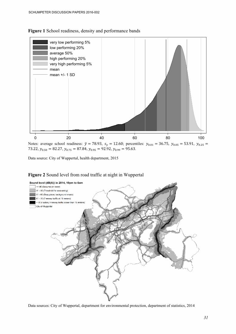
The performance bands in Figure 1 characterize five groups: the very low performing 5%, low

performing 20%, average 50%, high performing 20%, and the very high performing 5%. Av-

erage school readiness is 78.9% (SD = 12.6%) and the variable is left-skewed. The weakest

5% achieve only 54% school readiness, the medium 50% achieve 73%-88% school readiness.

In addition to information on abilities, there is a large set of background variables in

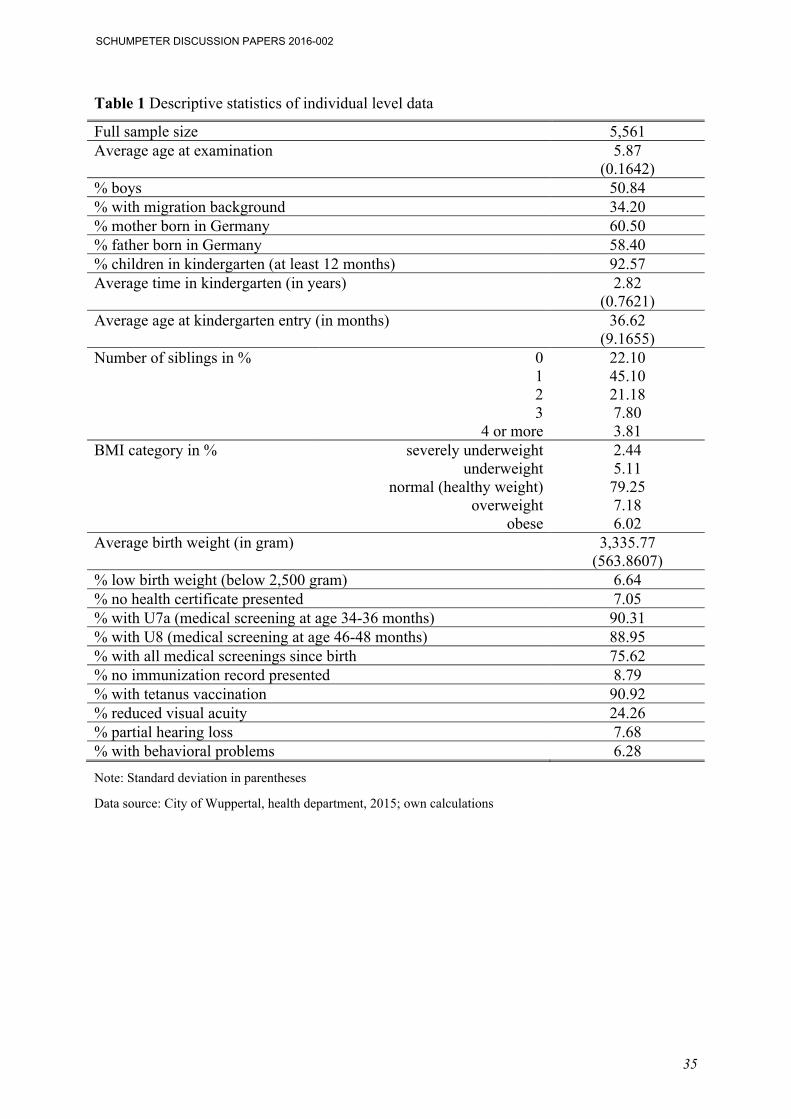
the SEnMed data. Table 1 summarizes the data. The sample comprises 5,561 children,

50.84% of whom are boys; 34.20% of the children are immigrants where migration status is

defined by the language spoken with the child during the first four years. If parents report a

language other than German, the child is said to have a migration background.

7 The overall KMO criterion is 0.8246; item KMO criteria lie between 0.7144 and 0.9098.


8

-- Table 1 about here --

On average, the children have attended kindergarten for 2.82 years (about 2 years and 10

months) before taking the exam. About 45% have one sibling; 3.81% have four or more sib-

lings. The share of overweight or obese children is larger than the share of (severely) under-

weight children. About 79% of the children have a healthy weight.

2.2. Noise pollution

The data on noise pollution is provided by the department for environmental protection of the

city of Wuppertal and the Federal Railway Authority (EBA, Eisenbahn-Bundesamt). In the

federal state of North-Rhine Westphalia, the municipalities are legally obligated to collect

data on noise exposure. Guidelines and requirements are specified by the Ministry for Climate

Protection, Environment, Agriculture, Conservation and Consumer Protection of the State of

North Rhine-Westphalia (MKULNV, Ministerium für Klimaschutz, Umwelt, Landwirtschaft,

Natur- und Verbraucherschutz des Landes Nordrhein-Westfalen) and are, therefore, standard-

ized and comparable. The reason for collecting the data is to measure the extent of noise pol-

lution and to develop state-wide concepts for noise reduction and noise protection. Common

structural measures for noise protection are soundproof walls, banks, tunnels or porous as-

phalt, the so-called quiet pavement, which absorbs sound better than regular asphalt. Between

2005 and 2014 the federal state of NRW invested about 506.1 Million Euros for noise protec-

tion and reconstruction at federal freeways (Autobahnen) (BMVI 2015). In addition, there

exist strict thresholds for tolerable noise exposure for new or extended freeways and after

reconstruction works. Noise levels at new or extended freeways must not exceed 49 dB(A) in

residential zones at night and 57 dB(A) after reconstruction (BMVI 2015). In comparison, the

noise levels of a quiet or standard conversation is 50 dB(A).


9

According to the guidelines of the MKULNV, the municipalities compute the extent

of ambient noise depending on its source (freeway (Autobahn), highway (Bundesstraße), in-

ner city road, railway, airport, industrial site, etc.) and the usage (e.g. traffic volume, maxi-

mum speed, type of asphalt, etc.). In addition, information on noise reducing or noise increas-

ing factors as well as noise abatement is taken into account, e.g. the natural topography, or

whether the road passes natural barriers or high buildings or the distance to soundproof walls.

The information on ambient noise is available for 2014 and comprises information on

noise during the day (6am to 10pm) and at night (10pm to 6am) collected between 2011 and

2014. Moreover, the data distinguishes noise from roads, from Wuppertal’s suspension rail-

way (Schwebebahn) and from the German Federal Railway. As noted earlier, in our analysis

we focus on the data available on noise at night. Of course, the noise level is lower at night

but it is even more likely to have a significant effect on health and cognitive development, as

it impairs the quality of sleep and regeneration (WHO 2009). This is in particular true for

children and elderly people. Moreover, children spend most of their time in the evening and at

night at home. Here, a noise level exceeding susurrus (about 40 dB(A)) is sufficient to wake

someone up (WHO 2009, p. XIII) and thus to cause disordered sleep.

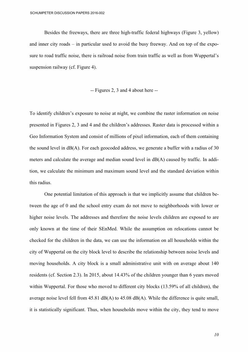
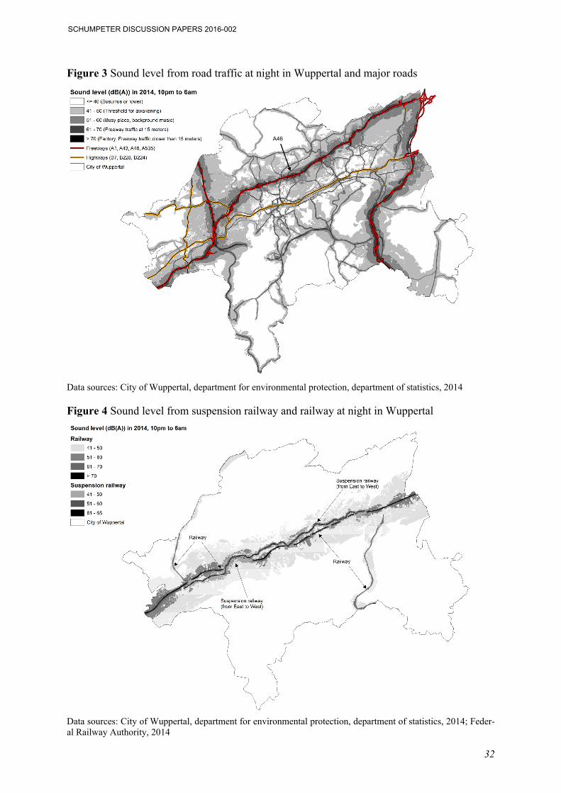
Due to its topography, traffic noise is of major concern in Wuppertal (see Figure 2 and

3) in particular at the so called ‘Talachse’ (valley axis) ranging from northeast to southwest.

The city of Wuppertal is divided by one of the high-traffic freeways in NRW, the A46 (Figure

3, red), which connects the Rhine area (Düsseldorf, Köln) with the Ruhr area (Dortmund, Bo-

chum, Essen). In the northeast of the city, the A46 connects with the A1 and A43, which are

another important freeways linking the Ruhr metropolitan region to Köln. In the southwest,

the A46 leads to the A535. In addition, the A46 is also considered a city freeway, which

means that it is not only used for long distance traffic. On average 71,600 vehicles per day use

the freeway passing through Wuppertal (BASt 2011).


10

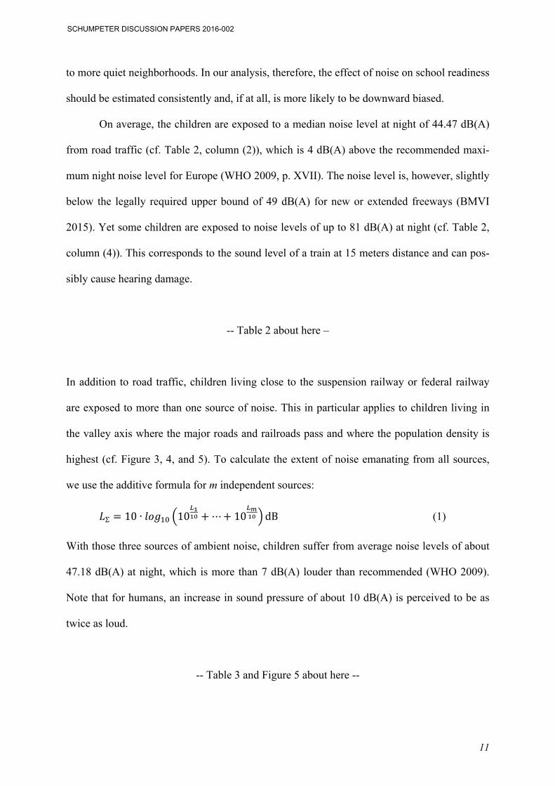
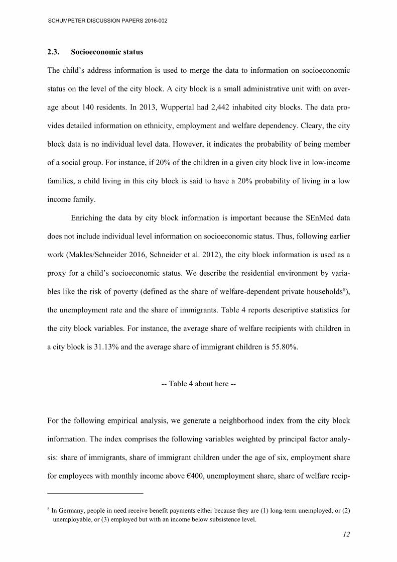
Besides the freeways, there are three high-traffic federal highways (Figure 3, yellow)

and inner city roads – in particular used to avoid the busy freeway. And on top of the expo-

sure to road traffic noise, there is railroad noise from train traffic as well as from Wuppertal’s

suspension railway (cf. Figure 4).

-- Figures 2, 3 and 4 about here --

To identify children’s exposure to noise at night, we combine the raster information on noise

presented in Figures 2, 3 and 4 and the children’s addresses. Raster data is processed within a

Geo Information System and consist of millions of pixel information, each of them containing

the sound level in dB(A). For each geocoded address, we generate a buffer with a radius of 30

meters and calculate the average and median sound level in dB(A) caused by traffic. In addi-

tion, we calculate the minimum and maximum sound level and the standard deviation within

this radius.

One potential limitation of this approach is that we implicitly assume that children be-

tween the age of 0 and the school entry exam do not move to neighborhoods with lower or

higher noise levels. The addresses and therefore the noise levels children are exposed to are

only known at the time of their SEnMed. While the assumption on relocations cannot be

checked for the children in the data, we can use the information on all households within the

city of Wuppertal on the city block level to describe the relationship between noise levels and

moving households. A city block is a small administrative unit with on average about 140

residents (cf. Section 2.3). In 2015, about 14.43% of the children younger than 6 years moved

within Wuppertal. For those who moved to different city blocks (13.59% of all children), the

average noise level fell from 45.81 dB(A) to 45.08 dB(A). While the difference is quite small,

it is statistically significant. Thus, when households move within the city, they tend to move


11

to more quiet neighborhoods. In our analysis, therefore, the effect of noise on school readiness

should be estimated consistently and, if at all, is more likely to be downward biased.

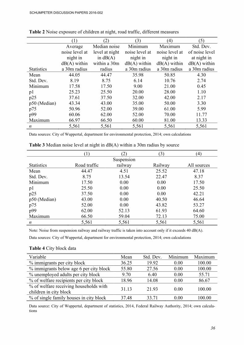
On average, the children are exposed to a median noise level at night of 44.47 dB(A)

from road traffic (cf. Table 2, column (2)), which is 4 dB(A) above the recommended maxi-

mum night noise level for Europe (WHO 2009, p. XVII). The noise level is, however, slightly

below the legally required upper bound of 49 dB(A) for new or extended freeways (BMVI

2015). Yet some children are exposed to noise levels of up to 81 dB(A) at night (cf. Table 2,

column (4)). This corresponds to the sound level of a train at 15 meters distance and can pos-

sibly cause hearing damage.

-- Table 2 about here –

In addition to road traffic, children living close to the suspension railway or federal railway

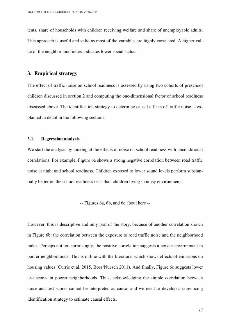
are exposed to more than one source of noise. This in particular applies to children living in

the valley axis where the major roads and railroads pass and where the population density is

highest (cf. Figure 3, 4, and 5). To calculate the extent of noise emanating from all sources,

we use the additive formula for m independent sources:

dB (1)

With those three sources of ambient noise, children suffer from average noise levels of about

47.18 dB(A) at night, which is more than 7 dB(A) louder than recommended (WHO 2009).

Note that for humans, an increase in sound pressure of about 10 dB(A) is perceived to be as

twice as loud.

-- Table 3 and Figure 5 about here --


12

2.3. Socioeconomic status

The child’s address information is used to merge the data to information on socioeconomic

status on the level of the city block. A city block is a small administrative unit with on aver-

age about 140 residents. In 2013, Wuppertal had 2,442 inhabited city blocks. The data pro-

vides detailed information on ethnicity, employment and welfare dependency. Cleary, the city

block data is no individual level data. However, it indicates the probability of being member

of a social group. For instance, if 20% of the children in a given city block live in low-income

families, a child living in this city block is said to have a 20% probability of living in a low

income family.

Enriching the data by city block information is important because the SEnMed data

does not include individual level information on socioeconomic status. Thus, following earlier

work (Makles/Schneider 2016, Schneider et al. 2012), the city block information is used as a

proxy for a child’s socioeconomic status. We describe the residential environment by varia-

bles like the risk of poverty (defined as the share of welfare-dependent private households8),

the unemployment rate and the share of immigrants. Table 4 reports descriptive statistics for

the city block variables. For instance, the average share of welfare recipients with children in

a city block is 31.13% and the average share of immigrant children is 55.80%.


For the following empirical analysis, we generate a neighborhood index from the city block

information. The index comprises the following variables weighted by principal factor analy-

sis: share of immigrants, share of immigrant children under the age of six, employment share

for employees with monthly income above €400, unemployment share, share of welfare recip-

8 In Germany, people in need receive benefit payments either because they are (1) long-term unemployed, or (2) unemployable, or (3) employed but with an income below subsistence level.


13

ients, share of households with children receiving welfare and share of unemployable adults.

This approach is useful and valid as most of the variables are highly correlated. A higher val-

ue of the neighborhood index indicates lower social status.

Empirical strategy

The effect of traffic noise on school readiness is assessed by using two cohorts of preschool

children discussed in section 2 and computing the one-dimensional factor of school readiness

discussed above. The identification strategy to determine causal effects of traffic noise is ex-

plained in detail in the following sections.

3.1. Regression analysis

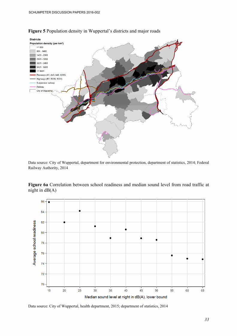
We start the analysis by looking at the effects of noise on school readiness with unconditional

correlations. For example, Figure 6a shows a strong negative correlation between road traffic

noise at night and school readiness. Children exposed to lower sound levels perform substan-

tially better on the school readiness tests than children living in noisy environments.

-- Figures 6a, 6b, and 6c about here --

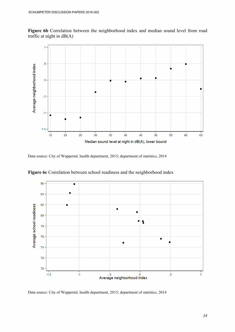
However, this is descriptive and only part of the story, because of another correlation shown

in Figure 6b: the correlation between the exposure to road traffic noise and the neighborhood

index. Perhaps not too surprisingly, the positive correlation suggests a noisier environment in

poorer neighborhoods. This is in line with the literature, which shows effects of emissions on

housing values (Currie et al. 2015, Boes/Nüesch 2011). And finally, Figure 6c suggests lower

test scores in poorer neighborhoods. Thus, acknowledging the simple correlation between

noise and test scores cannot be interpreted as causal and we need to develop a convincing

identification strategy to estimate causal effects.


14

3.1.1. Linear model and potential omitted variable bias

The equation to be estimated is

(2)

In eq. (2), is the outcome variable, i.e. school readiness of student i in cohort t, is a

vector of observed individual variables, like migration background, gender, number of sib-

lings, time in kindergarten, immunization record, early health conditions, or the neighborhood

variables. is unobserved innate ability. The variable is our measure of noise exposure,

e.g. the median sound level of traffic noise within a radius of 30m. is the unobserved fami-

ly background, like the parents’ valuation of education, the parents’ educational background

or the valuation of a quiet living environment. is a cohort fixed effect and is the error

term. Eq. (2) can be estimated by OLS which yields a consistent and unbiased estimate of ,

our coefficient of interest, as long as the unobserved is not correlated with the exposure to

noise, which, however, cannot be ruled out. The potential omitted variable bias can be written

as

, (3)

where is the vector of coefficients obtained from the regression of .on (An-

grist/Pischke 2009). We expect unobserved family background to be negatively related to

noise, because high income individuals can afford quiet housing and are willing to pay for

less noise exposure, thus . In eq. (2) , because higher status correlates positively

with higher school readiness. Thus, the estimated coefficient in (2) tends to overestimate the

true negative effect of noise on school readiness.

Moreover, innate ability is also unobserved which could be of potential concern

since we have no panel data. But, the problem of omitted variable bias due to unobserved in-

dividual ability is not substantial in the present setting as long as it can be assumed that innate

ability is not correlated with the way in which noise affects cognitive development. In other


15

words, noise is assumed to affect children of high ability just as it affects children of lower

ability.

The issue of unobserved innate ability known from the returns to education literature

comes up again, however, when estimating another important relationship: the effect of time

spent in kindergarten. The returns to education literature deals with two potential sources of

bias in this context: the omitted variable bias because of missing controls, like preferences,

and the problem that unobserved ability affects both the demand for education as well as the

outcome. The second source of endogeneity is not relevant in this paper. It is uncritical to

assume that parents in Germany enroll their children in kindergarten regardless of the child’s

ability. However, (unobserved) parental educational preferences as well the need of child care

might be important. It is unclear whether ambitious parents demand more time in kindergarten

or less, as kindergarten in Germany is not thought to be part of the schooling system; there is

no curriculum and attendance is voluntary. But more importantly, parents choose a kindergar-

ten that fits their preferences for kindergarten quality. Thus, the potential bias due to unob-

served kindergarten quality needs to be addressed.

3.1.2. Identification strategy

In a first step, we control for several observables by including comprehensive background

information from our rich data. The background information is available on the individual as

well as on the neighborhood level and can reduce the omitted variable bias resulting from

missing socioeconomic controls on the family level. However, educational preferences and

the child’s ability cannot be proxied by neighborhood information. And while time spent in

kindergarten is known, the effect of kindergarten duration is not easily identified because in

addition to unobserved parental input, the (unobserved) quality of the kindergarten will affect

cognitive development.


16

As noted above, children are enrolled in kindergarten for two reasons: First, parents

need day care and second, kindergarten has an educational purpose. Parents with strong pref-

erences for education will choose a kindergarten that fits their educational needs best. Our

strategy to deal with potential omitted variable bias in this case is as follows: First, besides

using the available individual level information, we control for characteristics on the city

block level. The information allows controlling for the ethnic composition, unemployment,

and welfare dependency rates. Since it can be reasonably assumed that families within a city

block are a fairly homogenous group, the unobserved part of the socioeconomic background

might not be as important to begin with if educational preferences are correlated with the ob-

served characteristics of the families, as is reasonable to assume. We also include a large set

of individual level control variables which are related to cognitive development. For example,

in addition to migration background and gender, we control for maturity effects, and family

related variables, like the number of siblings or the mother’s or father’s country of birth. We

control for health conditions or the number of health check-ups since birth. In addition, the

data comprises information on birth weight which is used as a proxy for early health condi-

tions.

In a next step and more importantly, we control for kindergarten fixed effects, , to

account for unobserved kindergarten quality. Furthermore, kindergarten fixed effects allow

controlling for the socioeconomic composition of the kindergarten as well as noise exposure

in kindergarten during the day. As mentioned in the introduction, noise exposure in kindergar-

ten might be substantial but also different across kindergartens. Since measures exposure

to noise at night and most children attend a kindergarten during the day, relying on noise at

night only results in measurement error if the noise level at night is a poor proxy for overall

(day and night) exposure to noise. Our data includes information on noise during the day and

at night, and it turns out that these noise levels at the children’s home are highly correlated.


17

In our setting, kindergarten fixed effects serve yet another purpose. Families are free

to choose a kindergarten, and kindergartens are fairly segregated (Makles/Schneider (2016)).

The diversity of kindergarten quality in Germany is large, since no curriculum for preschool

education exists. Kindergartens can be run by the municipalities, the church or by private ini-

tiatives (with or without public subsidies). Thus, the choice of the kindergarten also reflects

the socioeconomic status and in particular the unobserved educational preferences of the

families. This helps identifying the causal effect of noise on child development. Including

kindergarten fixed effects is expected to reduce the estimated negative noise effect, as we tend

to overestimate the detrimental effect due to the omitted variable bias. And finally, as the

child’s prospective primary school is known as well, additional school fixed effects, , can

be included in the analysis to even better control for parental educational preferences. Hence,

the equation to be estimated is modified to

, (4)

where the index denotes the kindergarten and denotes the school.

Besides identifying the noise effect, , kindergarten fixed effects also help to identify

the effect of kindergarten attendance. Recall that family preferences play a role when deciding

on the duration of kindergarten as well as the choice of the kindergarten. Those preferences

are accounted for by kindergarten and school fixed effects. Thus, identification of the kinder-

garten duration effect on school readiness stems from kindergarten and school fixed effects.

Nonetheless, full information on the child’s innate ability, educational preferences and educa-

tional inputs is missing; that might well affect the child’s cognitive outcome and also the

choice of residence which in turn correlates with the noise level in the neighborhood. There-

fore, some concerns about the exogeneity of exposure to noise at night remain even after con-

trolling for the full set of variables and kindergarten and primary school fixed effects. Hence,

in the following – but this is merely meant as a robustness check – we apply an instrumental

variables approach and test for endogeneity.


18

3.1.3. Robustness check

Since two variables are potentially endogenous, noise and time in kindergarten, both variables

need to be instrumented for. Our instrument for noise at night is the standard deviation of

noise at night within a radius of 100m (200m) around the child’s address, i.e. the variation in

the neighborhood. We use the exogenous variation in noise levels in the neighborhood to

identify the causal effect of permanent ambient noise on cognitive development. To be a valid

instrument, the instrument should correlate with noise but not affect a child’s cognitive ability

directly.

The main idea is to instrument the noise level at a child’s home by using information

on the neighbors. Noise levels are correlated within a neighborhood but there is no social sort-

ing within a radius of 100m (200m) around the child’s home. We argue that the standard de-

viation of noise exposure or the coefficient of variation within a neighborhood of 100m

(200m) is variation that is exogenous with respect to socioeconomic status. Families indeed

choose neighborhoods depending on the social composition and possibly the proximity to

good kindergartens, schools and green space. In addition, higher status families might choose

quieter environments. However, there is variation in noise exposure within a neighborhood

that cannot be fully controlled. Thus, families in the same neighborhood might be exposed to

different levels of noise although they are of similar socioeconomic background and have

similar educational preferences.

Time in kindergarten is instrumented by proxies for exogenous kindergarten supply

and legal rules on kindergarten admittance. The supply of kindergarten is measured by the

distance to the closest kindergarten. Legal rules help us to determine the theoretical kindergar-

ten age, i.e. the duration in kindergarten given the child enters kindergarten on his or her third

birthday. The theoretical kindergarten duration is used as an instrument, which has been prov-

en to be valid in school age studies (Bedard/Dhuey 2006, Mühlenweg/Puhani 2010, Jür-

ges/Schneider 2011). Unlike in school entry decisions, the rules are not as clear cut in case of


19

kindergarten. However, children in our data are entitled to attend kindergarten at the age of

three years. In addition, there is an older rule that the kindergarten year starts on August 1st

and all new children enter kindergarten on August 1st. While this rule is not legally binding, it

is still in practice and affects time in kindergarten depending on the month of birth. We there-

fore use assigned age (defined as 7 minus month of birth for children born between January

and July and 19 minus month of birth for children born between August and December (c.f.

Bedard/Dhuey 2006, p. 9)) as an additional instrument to describe the legal rules and to ad-

dress month of birth effects.

3.1.4. Varying treatment definition

Finally, the existing studies on the effects of noise do not explicitly analyze the functional

form of the relationship between noise and development. Noise is typically reported in decibel

A-weighted which is non-linear in loudness. Thus, even if the relationship between dB(A) and

development is linear, the relationship between loudness (subjective perception) and devel-

opment is not. We present some variations as a starting point for the discussion.

3.2. Cost-benefit analysis

To complete the analysis, we suggest an admittedly tentative cost-benefit analysis. As has

been noted earlier, public funds are being spent on noise protection and legal rules force gov-

ernments to engage in noise protection. While noise exposure might reduce cognitive devel-

opment, kindergarten education enhances development. The costs of various noise protection

measures are known. Once we have an estimate of the adverse effect of noise on cognitive

ability and an estimate of the school readiness improving effect of kindergarten attendance,

we can conduct a cost-benefit analysis. Hence, the main idea is to compensate the adverse

noise effect by additional education, the cost of which is known.


20

For doing so, we need an estimate of the cost of noise protection, for instance the cost

of a soundproof wall per km/year with depreciation period T, which we denote by noise. In

addition we need an estimate of the reduction in ambient noise resulting from the measure of

noise protection, dB(A) Those costs are compared with the cost of additional time in kinder-

garten kiga. With the estimated coefficients we can compute the relative effect on school

readiness as / kiga. Hence / kiga denotes the time spend in kindergarten (in months) that

has the same effect on school readiness as a one dB(A) reduction in noise. Multiplied by kiga

(per month), this gives the cost per child in kindergarten to match the effect of noise protec-

tion. Equating cost of noise protection per child and year, , times minus the reduction of

noise resulting from noise protection ( dB(A) to the alternative spending on kindergarten

education, allows solving for the critical number of children to benefit from noise protection,

N. This defines the breakeven point. Hence,

noisedB(A)

kigakiga

dB(A)

noise kiga

kiga (5)

The analysis is clearly simplifying at this point and partial in nature. However, we argue that

this presents a very conservative estimate. First, the focus is on early childhood development.

We know from the literature, that early childhood conditions are of importance for later life

development. Hence, we tend to underestimate the benefit from noise protection. However,

since we compare benefits from lower noise levels with effects from attending kindergarten,

which is also thought to have a long term effect, the bias might not be severe after all. Second,

and more importantly, we do not account for the effects on other individuals in the neighbor-

hood. Adults, younger and older children benefit as well. In particular for the adult popula-

tion, the evidence for severe health effects of noise is compelling (EEA 2014).


21

Regression results

4.1. OLS Estimates

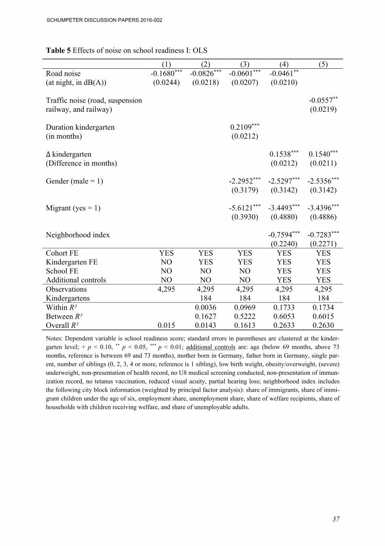
Table 5 summarizes the regression results. As the dependent variable, our index of school

readiness, is between 0 and 100, the effects of all variables can be interpreted as changes in

school readiness in percentage points (or in %).


As argued above, we expect the adverse effect of noise measured by the median sound level

from road traffic in dB(A) at night to be overestimated due to the omitted variable bias. In

fact, the noise coefficient in our basic model without fixed effects (cf. Table 5, column (1)) is

twice as large as the coefficient when accounting for kindergarten fixed effects (column (2)).

The effect decreases from -0.168 to -0.083. However, it remains significant on the 1% level.

Children living in noisy environments perform worse on the school entry examination than

children living in quiet areas. Adding individual controls (column (3)) like kindergarten dura-

tion, gender and migration status reduces the estimated effect slightly. However, changes are

not substantial and the effect of noise from road traffic on school readiness remains negative

and significant at the 1% level. All included controls have the expected effect on school read-

iness. Immigrant status, for instance, has the expected strong negative effect whereas time

spent in kindergarten has a positive effect.

To further control for individual characteristics and the families’ socioeconomic sta-

tus, we add additional controls along with health variables in model (4). The health variables

include dummy coded information on low birth weight, overweight/obese, partial hearing

loss, and reduced visual acuity and the number of medical screenings since birth. These varia-

bles indicate physical health which may affect school readiness and some of them also capture

the socioeconomic status of the family. Socioeconomic status (SES) and some of the health


22

variables chosen in the analysis are correlated. Higher SES children are less likely to be

obese, have higher birth weight and are more likely to attend the recommended medical

screenings. The model in column (4) also includes the neighborhood index which uses the city

block data and describes the socioeconomic structure of the neighborhood as discussed in

section 2.3. The index of low SES of the neighborhood has the expected negative and signifi-

cant impact. Since high values represent low SES, low SES goes along with lower school

readiness. Finally, we need to address another variable: the duration in kindergarten. Since

kindergarten is an educational institution that aims at fostering children’s cognitive develop-

ment, time spent in kindergarten is an important variable to explain school readiness. But

clearly, the variable has two potential problems. First, we are aware of the aforementioned

omitted variable bias, which we address by kindergarten and school fixed effects as well as

the individual and neighborhood controls in model (4). Second, the variable might measure

maturity effects because children who are older at the school entry exam might outperform

the younger peers. Even though this is not a systematic problem in Wuppertal, since children

are invited to the school entry exam according to birth date and are about 69 to 73 months old

when examined, we address this issue in model (4) by adding two dummy variables for chil-

dren that are younger than 69 months and children who are older than 73 months. In addition,

we compute the theoretical kindergarten duration (age at examination minus 36 months) and

use the variable kindergarten which is the difference between time in kindergarten and the

theoretical time in kindergarten in the regression. The effect of time in kindergarten drops in

model (4) to 0.154 but remains significant at the 1% level.

In models (1) to (4) we focus on noise from road traffic only. But, since noise pollu-

tion does not only result from road traffic, but also includes railroads and other rail vehicles,

like trams or the suspension railway in Wuppertal, we compute the overall noise level as de-

scribed in Section 2.3 and use it as the treatment variable in column (5). The effect of ambient


23

noise on school readiness is now slightly stronger with -0.056 than the effect of road traffic

only. The coefficients of the controls remain essentially unaffected.

4.2. IV Estimates

As discussed in Section 3.1, the data might not include all desirable individual level infor-

mation like parents’ education or educational preferences. While we are confident that our

identification strategy identifies the causal effect of noise on school readiness, we suggest a

robustness check and perform an IV estimation approach using the instruments as discussed in

section 3.1.3 and check the exogeneity of the treatment assumption in the models of Table 5.

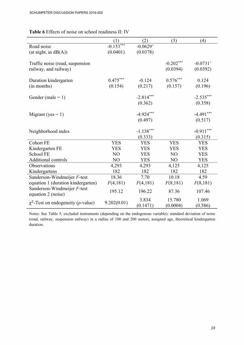
Table 6 summarizes the results for this robustness check. In model (1), the only con-

trols are kindergarten duration, the kindergarten fixed effects and the cohort fixed effect. Road

noise as well as kindergarten duration affect school readiness significantly. The reported first

stage multivariate F-statistics are the Sanderson-Windmeijer test on weak identification

(Sanderson/Windmeijer 2015). The test on endogeneity which compares OLS with IV rejects

the null hypothesis of no endogeneity. Model (2) is the full model as specified in Table 5,

column (4). The coefficients drop and the coefficient for kindergarten duration is no longer

significant. The noise variable drops and is close to the OLS specification in Table 5 but only

marginally significant. The test on endogeneity no longer rejects the null hypothesis of exog-

eneity. Hence our conjecture that the specification in Table 5, column (4) adequately address-

es the omitted variable bias is supported. In models (3) and (4), the noise variable includes

noise from road traffic, railway traffic and the suspension railway. The conclusions are similar

to the model with road traffic only. While our models pass the tests on identification and the

instruments are not weak according to the method proposed in Sanderson/Windmeijer (2015),

the null hypothesis of exogeneity of the regressors cannot be rejected in the full models. Thus,

our strategy to identify the effect by a saturated model with kindergarten and school fixed

effects (cf. Table 5, column (4) and (5)) is supported.


24

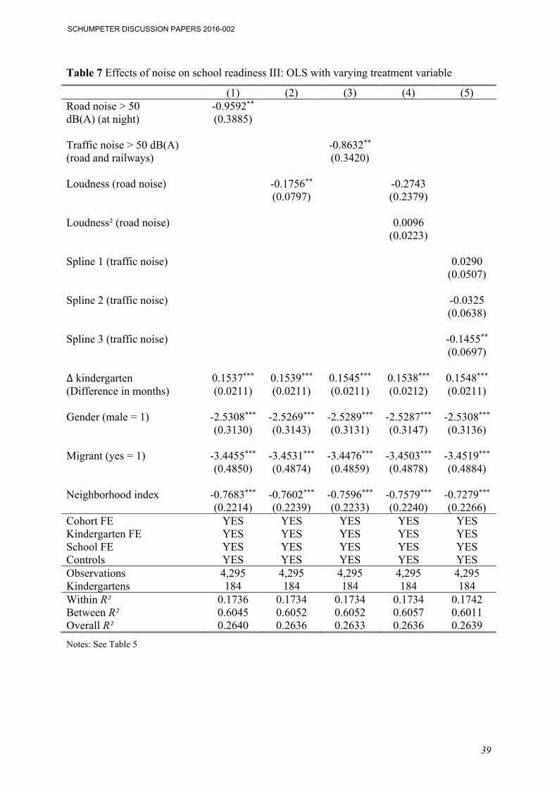
4.3. Estimates for different specifications of the treatment variables

Table 7 extends the analysis to different specifications of the noise variables. Noise is meas-

ured in dB(A) which is not a linear measure of experienced loudness. An increase of 10

dB(A) amounts to a doubling of the noise level. While there is no exact formula to translate

dB(A) in loudness, the approximate relationship is

dB(A) (6)

Since the relationship between dB(A) and loudness is not linear, the effect of noise on child

development is not linear either, even if the effect of noise measured in dB(A) on develop-

ment is linear. Moreover, low levels of noise are not harmful, but high levels are. Identifying

a threshold beyond which noise is harmful is clearly beyond the scope of this study. However,

in Table 7 we provide some first evidence on how various measures of noise affect school

readiness. The models reported there include the controls as in Table 5, model (4). Only the

noise variable differs between the models. In column (1) the noise variable is a dummy which

has a value of one if the noise level exceeds 50 dB(A), a commonly used threshold for ad-

verse health effects of noise. The effect is strong, negative and significant. Compared to the

effect of kindergarten attendance, the effect is more than 6 months in kindergarten or about

one half of the gender difference. Put differently, children who are exposed to permanent high

levels of noise at night are about half a kindergarten year behind. In model (2) the measure of

loudness (cf. eq. (6)) is used, and specification (3) uses the level of traffic noise from all

sources instead of road noise only. The effects are rather similar. Including loudness and

loudness squared in model (4) eliminates any significant effects due to high multicollinearity.

In model (5) we finally estimate a spline model with 3 splines (the noise is measured in dB(A)

and includes all sources (road, railway and suspension railway)). The significant effect is only

at the last spline. The first two splines are insignificant. Thus, the adverse effect of noise does

in fact occur only at higher levels of noise. Public spending on noise reduction might there-


25

fore be well advised to focus on regions with severe ambient noise levels with more than 50

dB(A) at night.

How much to spend on noise abatement?

Noise protection is high on the political agenda. While the cost of investing in noise abate-

ment should be readily available, the benefits are hard to grasp. At this point, and using our

data, we cannot provide a full cost-benefit analysis. However, we can use our results to com-

pare the cost of the adverse effects of ambient noise on child development with the cost of

noise protection measures such as walls or quiet pavement. Using our estimates of the adverse

effects of noise on child development in Table 5, column (4), we can compute the breakeven

points as discussed in Section 3.2.

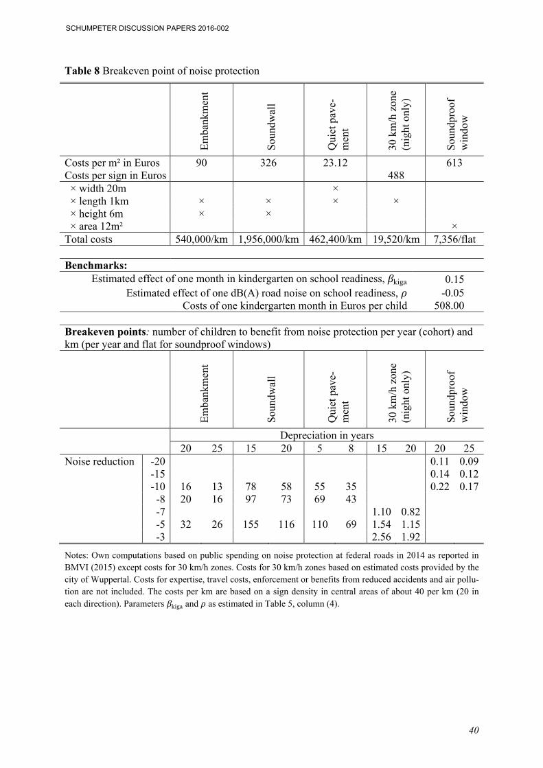
Table 8 summarizes the results for examples of noise abatement methods: noise pro-

tection embankment and soundwalls as protection measures at highways and quiet pavement

and 30 km/h zones in inner city areas. In addition, we do calculations for soundproof win-

dows, a passive noise protection method. Soundproof windows and 30 km/h zones are suita-

ble to reduce noise from inner city roads, where other abatement measures like soundproof

walls are not an option.


Provided the resulting reduction in noise is 10 dB(A) and the depreciation period is 20 years,

the breakeven point for an investment in noise protection embankment is reached for 16 chil-

dren per km and cohort. With an investment in soundwalls, the number of children is 58. As-

suming a shorter depreciation period of 15 years only, the number of children rises to 78.

Quiet pavement is less expensive, although the costs vary depending on the location (BMVI,

2015) and the durability is still uncertain. For a depreciation period of 8 years the breakeven


26

point is reached at 35 children. If the pavement is less durable, i.e. only 5 years, the number of

children is 55. As shown in Table 8, those figures are less favorable, if the noise reduction is

only 8 or 5 dB(A). Given a reduction in noise of 5 dB(A) only and a depreciation period of 15

years, the soundwall breaks even at 155 children per cohort and km.

Establishing a 30 km/h zone comes at lower monetary costs but it is very unpopular as

it slows down traffic. The costs in Table 8 only include costs for setting up the street signs.

Additional time costs or enforcement costs are not included. The same applies to additional

benefits from reduced local air pollution or fewer accidents. Reducing speed limit from 50

km/h to 30 km/h within a urban area reduces the noise level between 3 dB(A) and 7 dB(A).

Assuming a reduction of 3 dB(A) and a depreciation period of 20 years, 30 km/h signs break

even at 1.92 children per cohort and km. But clearly, without knowing the time costs, this

estimate is not sufficiently reliable.

In addition to active noise protection measures, we also compute the breakeven point

for soundproof windows. Soundproof windows can absorb additional 10 dB(A) or even up to

25 dB(A) compared to a standard window9 and cost on average 613 Euros/m2 (BMVI 2015).10

Hence, soundproof windows effectively reduce noise form inner city traffic at night. Assum-

ing an average flat with about 4 to 6 windows, an area of 12m² has to be equipped with

soundproof windows. With a noise reduction of 20 dB(A) and a depreciation period of 25

years this investment breaks even at 0.09 children per flat and year. In the less favorite case

with a depreciation period of 20 years and a noise reduction of 10 dB(A), the number is at

0.22 children per flat and year. Put differently, in the less favorite case the windows have to

protect a newborn every 4.5 years per flat from noise. Given that about 150.000 households

are suffering from severe inner city traffic (about ¾ of all flats in Wuppertal), even in the fa-

vorite case (-20 dB(A), 25 years) the breakeven point is reached at 13,500 children per cohort,

9 According to the VDI guideline 2719 of the German Engineers Association (Verein Deutscher Ingenieure) 10 Note that additional cost for ventilation are not included.


27

which is far more than a cohort size in Wuppertal. Or alternatively, given that the costs of

soundproof windows are 7,356 per flat and the noise abatement of 20 dB(A) has the same

effect as 6.66 month in kindergarten, the benefits are worth 3,383 Euros. Hence if there are

2.17 children per family and flat (over a time period of 25 years), the investments breaks

even.

These computations can only serve as a starting point for the discussion. There are cer-

tainly some caveats besides the limited selection of noise abatement instruments in the analy-

sis. For instance, the depreciation periods are estimates. If quiet pavement is not as long last-

ing as 5 years, the results change. Also, when looking at the cost of embankments, we under-

estimate the true costs, because in an urban area like Wuppertal, embankments are even more

expensive than soundwalls simply because of limited space. In fact, in densely populated are-

as embankments might not be a realistic option in the first place and a mix of different

measures, like quiet pavement, soundproof windows and 30 km/h zones has to be discussed.

But keeping the limitations in mind, the computations show that breakeven points can be cal-

culated for all types of active and passive noise abatement instruments as long as their costs

are known. And, as noted earlier, this is a conservative estimate, as other groups of the popu-

lation also benefit from reduced noise levels but are not included in our calculations.

A glance at Figure 5 suggests that the population density is high close to the highways

and freeways around the valley axis of Wuppertal (running from northeast to southwest). As-

suming a density of 5,000 inhabitants per km2 and 1% of the population being one school co-

hort, our estimates suggest to invest in noise abatement around the valley axis of Wuppertal,

but possibly not to invest at the roads in the northwestern or southeastern part of the city, un-

less embankments are an option.


28

Conclusion and Discussion

Noise pollution is detrimental to health and to cognitive development of children. This is not

only true for extreme level of noise, like noise from an airport, but also for traffic noise in a

typical urban area. Using a census of preschool children of a city in Germany, this paper

shows that children who are exposed to permanent traffic noise during the night fall signifi-

cantly behind in terms of school readiness. Being exposed to 10 dB(A) additional noise elimi-

nates the positive effect on school readiness of about 3 months in kindergarten. Moreover, the

effect becomes stronger for children who are exposed to permanent noise levels higher than

50 dB(A) at night. We contribute to the literature and the policy debate by working with ad-

ministrative data and focusing on the everyday exposure to noise instead of looking at case

studies with exceptionally high levels of noise. Possible policy instruments are either publicly

provided noise abatement, like soundwalls and quiet pavement, or legal rules like 30 km/h

zones. In this paper, we assess the public cost of five different abatement instruments and

compare them to the benefits. It turns out that abatement in densely populated urban areas of

about 3,000 to 5,000 per km2 can be cost efficient, even with a conservative assessment of the

benefits.

Acknowledgments

We gratefully acknowledge support by several departments of the city of Wuppertal in partic-

ular for granting access to SEnMed, road traffic noise, suspension railway noise, and city

block data. Data on railway noise by courtesy of the German Federal Railway Authority.

References

Angrist, J. D.; Pischke, J.-S. (2009): Mostly Harmless Econometrics. New Jersey: Princeton University Press.

Babisch W. (2003): Stress Hormones in the Research on Cardiovascular Effects of Noise. In: Noise Health, 5(18), 1-11.


29

Babisch, W.; Neuhauser, H.; Thamm, M.; Seiwert, M. (2009): Blood Pressure of 8-14 Year Old Children in Relation to Traffic Noise at Home – Results of the German Environ-mental Survey for Children (GerES IV). In: Science of the Total Environment, 407(22), 5839-5843.

BASt - Bundesanstalt für Straßenwesen (2011): Manuelle Straßenverkehrszählung 2010. [LINK]

Bedard, K. and Dhuey, E. (2006): The Persistence of Early Childhood Maturity: International Evidence of Long-Run Age Effects. In: Quarterly Journal of Economics 121, 1437–1472.

BMVI - Bundesministerium für Verkehr und digitale Infrastruktur (eds.) (2015): Statistik des Lärmschutzes an Bundesfernstraßen 2014. Bonn: BMVI. [LINK]

Boes, S.; Nüesch, S.; (2011): Quasi-experimental evidence on the effect of aircraft noise on apartment rents. In: Journal of Urban Economics, 69(2), 196-204.

Clark, C.; Martin, R.; Kempen, E. v.; Alfred, T.; Head, J.; Davies, H. W.; Haines, M. M.; Lopez Barrio, I.; Matheson, M.; Stansfeld, S. A. (2006): Exposure-Effect Relations be-tween Aircraft and Road Traffic Noise Exposure at School and Reading Comprehen-sion. In: American Journal of Epidemiology, 163(1), 27-37.

Cohen, S.; Evans, G. W.; Krantz, D. S.; Stokols, D. (1980): Physiological, Motivational, and Cognitive Effects of Aircraft Noise on Children. In: American Psychologist, 35(3), 231-243.

Cohen, S.; Glass, D. C.; Singer, J. E. (1973): Apartment Noise, Auditory Discrimination, and Reading Ability in Children. In: Journal of Experimental Social Psychology, 9(5), 407-422.

Coneus, K.; Spiess, C. K. (2012): Pollution exposure and child health: Evidence for infants and toddlers in Germany. In: Journal of Health Economics, 31(1), 180-196.

Currie, J.; Davis, L.; Greenstone, M.; Walker, R. (2015): Environmental Health Risks and Housing Values: Evidence from 1,600 Toxic Plant Openings and Closings. In: Ameri-can Economic Review, 105(2), 678-709.

Currie, J.; Graff Zivin, J. S.; Mullins, J; Neidell, M. J. (2014): What Do We Know About Short- and Long-Term Effects of Early-Life Exposure to Pollution? In: Annual Review of Resource Economics, 6, 217-247.

EEA - European Environment Agency (2014): Noise in Europe 2014, EEA Report No 10/2014, doi:10.2800/763331.

Houthuijs, D. J. M.; van Beek; A. J.; Swart, W. J. R.; van Kempen, E. E. M. M. (2014): Health implication of road, railway and aircraft noise in the European Union. Provision-al results based on the 2nd round of noise mapping, RIVM Report 2014-0130. [LINK]

Hygge, S.; Evans, G. W.; Bullinger, M. (2002): A Prospective Study of Some Effects of Air-craft Noise on Cognitive Performance in Schoolchildren. In: Psychological Science, 13(5), 469-474.

Jürges, H.; Schneider, K. (2011): Why young boys stumble: Early tracking, age and gender bias in the German school system. In: German Economic Review, 12(4), 371-394.


30

Lercher, P.; Evans, G. W.; Meis, M.; Kofler W. W. (2002): Ambient Neighborhood Noise and Children’s Mental Health. In: Occupational & Environmental Medicine, 59(6), 380-386.

Makles, A.; Schneider, K. (2016): Extracurricular educational programs and school readiness: evidence from a quasi-experiment with preschool children. In: Empirical Economics (forthcoming).

Mühlenweg, A. M.; Puhani, P. A. (2010): The Evolution of the School-Entry Age Effect in a School Tracking System. In: Journal of Human Resources, 45(2), 407-438.

Öhrström, E.; Skånberg, A.; Svensson, H.; Gidlöf-Gunnarsson (2006): Effects of road traffic noise and the benefit of access to quietness. In: Journal of Sound and Vibration. 295(1-2), 40-59.

Rosenberg, J. (1991): Jets over Labrador and Quebec: Noise Effects on Human Health. In: Canadian Medical Association Journal, 144(7), 869-875.

Sanderson, E.; Windmeijer, F. (2015): A Weak Instrument F-Test in Linear IV Models with Multiple Endogenous Variables. In: Journal of Econometrics, doi: 10.1016/j.jeconom.2015.06.004.

Schneider, K.; Schuchart, C.; Weishaupt, H.; Riedel, A. (2012): The effect of free primary school choice on ethnic groups - Evidence from a policy reform. In: European Journal of Political Economy, 28(4), 430-444.

Stansfeld, S. A.; Berglund, B.; Clark, C.; Lopez Barrio, I.; Fischer, P.; Öhrström, E.; Haines M. M.; Head, J.; Hygge, S.; Kamp, I. v.; Berry, B. F. (2005): Aircraft Noise and Road Traffic Noise and Children’s Cognition and Health: a cross-national study. In: Lancet, 365(9475), 1942-1949.

Tamburlini, G. (2002): Environmental hazards in specific settings and media: an overview. In: Tamburlini, G.; Ehrenstein, O. S. v.; Berollini, R. (eds.): Children’s health and envi-ronment: A review of evidence. Copenhagen: European Environment Agency & World Health Organziation, 29-42.

WHO – World Health Organization (2009): Night Noise Guidelines for Europe. Copenhagen: World Health Organization.

WHO – World Health Organization (2011): Burden of Disease from Environmental Noise: Quantification of Healthy Life Years Lost in Europe. Copenhagen: World Health Or-ganization.


31

Figure 1 School readiness, density and performance bands

Notes: average school readiness: , ; percentiles: . . , .

, . , . , . , . .

Data source: City of Wuppertal, health department, 2015

Figure 2 Sound level from road traffic at night in Wuppertal

Data sources: City of Wuppertal, department for environmental protection, department of statistics, 2014

0 20 40 60 80 100

very low performing 5%low performing 20%average 50%high performing 20%very high performing 5%meanmean +/- 1 SD


32

Figure 3 Sound level from road traffic at night in Wuppertal and major roads

Data sources: City of Wuppertal, department for environmental protection, department of statistics, 2014

Figure 4 Sound level from suspension railway and railway at night in Wuppertal

Data sources: City of Wuppertal, department for environmental protection, department of statistics, 2014; Feder-al Railway Authority, 2014

A46


33

Figure 5 Population density in Wuppertal’s districts and major roads

Data source: City of Wuppertal, department for environmental protection, department of statistics, 2014; Federal Railway Authority, 2014

Figure 6a Correlation between school readiness and median sound level from road traffic at night in dB(A)

Data source: City of Wuppertal, health department, 2015; department of statistics, 2014


34

Figure 6b Correlation between the neighborhood index and median sound level from road traffic at night in dB(A)


Figure 6c Correlation between school readiness and the neighborhood index



35

Table 1 Descriptive statistics of individual level data

Full sample size 5,561 Average age at examination 5.87 (0.1642) % boys 50.84 % with migration background 34.20 % mother born in Germany 60.50 % father born in Germany 58.40 % children in kindergarten (at least 12 months) 92.57 Average time in kindergarten (in years) 2.82 (0.7621) Average age at kindergarten entry (in months) 36.62 (9.1655) Number of siblings in % 0 22.10

1 45.10 2 21.18 3 7.80

4 or more 3.81 BMI category in % severely underweight 2.44

underweight 5.11 normal (healthy weight) 79.25

overweight 7.18 obese 6.02

Average birth weight (in gram) 3,335.77 (563.8607) % low birth weight (below 2,500 gram) 6.64 % no health certificate presented 7.05 % with U7a (medical screening at age 34-36 months) 90.31 % with U8 (medical screening at age 46-48 months) 88.95 % with all medical screenings since birth 75.62 % no immunization record presented 8.79 % with tetanus vaccination 90.92 % reduced visual acuity 24.26 % partial hearing loss 7.68 % with behavioral problems 6.28

Note: Standard deviation in parentheses

Data source: City of Wuppertal, health department, 2015; own calculations


36

Table 2 Noise exposure of children at night, road traffic, different measures

(1) (2) (3) (4) (5)

Statistics

Average noise level at

night in dB(A) within a 30m radius

Median noise level at night

in dB(A) within a 30m

radius

Minimum noise level at


Maximum noise level at


Std. Dev. of noise level

at night in dB(A) within a 30m radius

Mean 44.05 44.47 35.98 50.85 4.30 Std. Dev. 8.19 8.75 6.14 10.76 2.74 Minimum 17.58 17.50 9.00 21.00 0.45 p1 25.23 25.50 20.00 28.00 1.10 p25 37.61 37.50 32.00 42.00 2.17 p50 (Median) 43.34 43.00 35.00 50.00 3.30 p75 50.96 52.00 39.00 61.00 5.99 p99 60.06 62.00 52.00 70.00 11.77 Maximum 66.97 66.50 60.00 81.00 13.33 n 5,561 5,561 5,561 5,561 5,561

Data sources: City of Wuppertal, department for environmental protection, 2014; own calculations

Table 3 Median noise level at night in dB(A) within a 30m radius by source

(1) (2) (3) (4)

Statistics Road traffic Suspension

railway Railway All sources Mean 44.47 4.51 25.52 47.18 Std. Dev. 8.75 13.54 22.47 8.37 Minimum 17.50 0.00 0.00 17.50 p1 25.50 0.00 0.00 25.50 p25 37.50 0.00 0.00 42.21 p50 (Median) 43.00 0.00 40.50 46.64 p75 52.00 0.00 43.82 53.27 p99 62.00 52.13 61.93 64.60 Maximum 66.50 59.04 72.13 75.00 n 5,561 5,561 5,561 5,561

Note: Noise from suspension railway and railway traffic is taken into account only if it exceeds 40 dB(A).

Data sources: City of Wuppertal, department for environmental protection, 2014; own calculations

Table 4 City block data

Variable Mean Std. Dev. Minimum Maximum % immigrants per city block 36.25 19.92 0.00 100.00 % immigrants below age 6 per city block 55.80 27.56 0.00 100.00 % unemployed adults per city block 9.70 6.40 0.00 55.71 % of welfare recipients per city block 18.96 14.08 0.00 86.67 % of welfare receiving households with children in city block

31.13 21.93 0.00 100.00

% of single family houses in city block 37.48 33.71 0.00 100.00

Data source: City of Wuppertal, department of statistics, 2014, Federal Railway Authority, 2014; own calcula-tions


37

Table 5 Effects of noise on school readiness I: OLS

(1) (2) (3) (4) (5) Road noise -0.1680*** -0.0826*** -0.0601*** -0.0461** (at night, in dB(A)) (0.0244) (0.0218) (0.0207) (0.0210) Traffic noise (road, suspension -0.0557** railway, and railway) (0.0219) Duration kindergarten 0.2109*** (in months) (0.0212)

kindergarten 0.1538*** 0.1540*** (Difference in months) (0.0212) (0.0211) Gender (male = 1) -2.2952*** -2.5297*** -2.5356*** (0.3179) (0.3142) (0.3142) Migrant (yes = 1) -5.6121*** -3.4493*** -3.4396*** (0.3930) (0.4880) (0.4886) Neighborhood index -0.7594*** -0.7283*** (0.2240) (0.2271) Cohort FE YES YES YES YES YES Kindergarten FE NO YES YES YES YES School FE NO NO NO YES YES Additional controls NO NO NO YES YES Observations 4,295 4,295 4,295 4,295 4,295 Kindergartens 184 184 184 184 Within R² 0.0036 0.0969 0.1733 0.1734 Between R² 0.1627 0.5222 0.6053 0.6015 Overall R² 0.015 0.0143 0.1613 0.2633 0.2630

Notes: Dependent variable is school readiness score; standard errors in parentheses are clustered at the kinder-garten level; + p < 0.10, ** p < 0.05, *** p < 0.01; additional controls are: age (below 69 months, above 73 months, reference is between 69 and 73 months), mother born in Germany, father born in Germany, single par-ent, number of siblings (0, 2, 3, 4 or more, reference is 1 sibling), low birth weight, obesity/overweight, (severe) underweight, non-presentation of health record, no U8 medical screening conducted, non-presentation of immun-ization record, no tetanus vaccination, reduced visual acuity, partial hearing loss; neighborhood index includes the following city block information (weighted by principal factor analysis): share of immigrants, share of immi-grant children under the age of six, employment share, unemployment share, share of welfare recipients, share of households with children receiving welfare, and share of unemployable adults.


38

Table 6 Effects of noise on school readiness II: IV

(1) (2) (3) (4) Road noise -0.153*** -0.0629+ (at night, in dB(A)) (0.0401) (0.0378) Traffic noise (road, suspension -0.202*** -0.0731+ railway, and railway) (0.0394) (0.0392) Duration kindergarten 0.475*** -0.124 0.576*** 0.124 (in months) (0.154) (0.217) (0.157) (0.196) Gender (male = 1) -2.814*** -2.535*** (0.362) (0.358) Migrant (yes = 1) -4.924*** -4.491*** (0.497) (0.517) Neighborhood index -1.138*** -0.911*** (0.333) (0.315) Cohort FE YES YES YES YES Kindergarten FE YES YES YES YES School FE NO YES NO YES Additional controls NO YES NO YES Observations 4,293 4,293 4,125 4,125 Kindergartens 182 182 182 182 Sanderson-Windmeijer F-test equation 1 (duration kindergarten)

18.36 F(4,181)

7.70 F(4,181)

10.18 F(8,181)

4.59 F(8,181)

Sanderson-Windmeijer F-test equation 2 (noise)

195.12 196.22 87.36 107.46

-Test on endogeneity (p-value) 9.202(0.01) 3.834

(0.1471) 15.780

(0.0004) 1.069

(0.586)

Notes: See Table 5; excluded instruments (depending on the endogenous variable): standard deviation of noise (road, railway, suspension railway) in a radius of 100 and 200 meters, assigned age, theoretical kindergarten duration.


39

Table 7 Effects of noise on school readiness III: OLS with varying treatment variable

(1) (2) (3) (4) (5) Road noise > 50 -0.9592** dB(A) (at night) (0.3885) Traffic noise > 50 dB(A) -0.8632** (road and railways) (0.3420) Loudness (road noise) -0.1756** -0.2743 (0.0797) (0.2379) Loudness² (road noise) 0.0096 (0.0223) Spline 1 (traffic noise) 0.0290 (0.0507) Spline 2 (traffic noise) -0.0325 (0.0638) Spline 3 (traffic noise) -0.1455** (0.0697)

kindergarten 0.1537*** 0.1539*** 0.1545*** 0.1538*** 0.1548*** (Difference in months) (0.0211) (0.0211) (0.0211) (0.0212) (0.0211) Gender (male = 1) -2.5308*** -2.5269*** -2.5289*** -2.5287*** -2.5308*** (0.3130) (0.3143) (0.3131) (0.3147) (0.3136) Migrant (yes = 1) -3.4455*** -3.4531*** -3.4476*** -3.4503*** -3.4519*** (0.4850) (0.4874) (0.4859) (0.4878) (0.4884) Neighborhood index -0.7683*** -0.7602*** -0.7596*** -0.7579*** -0.7279*** (0.2214) (0.2239) (0.2233) (0.2240) (0.2266) Cohort FE YES YES YES YES YES Kindergarten FE YES YES YES YES YES School FE YES YES YES YES YES Controls YES YES YES YES YES Observations 4,295 4,295 4,295 4,295 4,295 Kindergartens 184 184 184 184 184 Within R² 0.1736 0.1734 0.1734 0.1734 0.1742 Between R² 0.6045 0.6052 0.6052 0.6057 0.6011 Overall R² 0.2640 0.2636 0.2633 0.2636 0.2639

Notes: See Table 5


40

Table 8 Breakeven point of noise protection

Em

bank

men

t

Sou

ndw

all

Qui

et p

ave-

men

t

30 k

m/h

zon

e (n

ight

onl

y)

Sou

ndpr

oof

win

dow

Costs per m² in Euros 90 326 23.12 613 Costs per sign in Euros 488 × width 20m × × length 1km × × × × × height 6m × × × area 12m² × Total costs 540,000/km 1,956,000/km 462,400/km 19,520/km 7,356/flat Benchmarks:

Estimated effect of one month in kindergarten on school readiness, kiga 0.15 Estimated effect of one dB(A) road noise on school readiness, -0.05

Costs of one kindergarten month in Euros per child 508.00 Breakeven points: number of children to benefit from noise protection per year (cohort) and km (per year and flat for soundproof windows)

Em

bank

men

t

Sou

ndw

all

Qui

et p

ave-

men

t

30 k

m/h

zon

e (n

ight

onl

y)

Sou

ndpr

oof

win

dow

Depreciation in years 20 25 15 20 5 8 15 20 20 25 Noise reduction -20 0.11 0.09 -15 0.14 0.12 -10 16 13 78 58 55 35 0.22 0.17 -8 20 16 97 73 69 43 -7 1.10 0.82 -5 32 26 155 116 110 69 1.54 1.15 -3 2.56 1.92

Notes: Own computations based on public spending on noise protection at federal roads in 2014 as reported in BMVI (2015) except costs for 30 km/h zones. Costs for 30 km/h zones based on estimated costs provided by the city of Wuppertal. Costs for expertise, travel costs, enforcement or benefits from reduced accidents and air pollu-tion are not included. The costs per km are based on a sign density in central areas of about 40 per km (20 in each direction). Parameters kiga and as estimated in Table 5, column (4).


SCHUMPETER DISCUSSION PAPERS Quiet please! Adverse...

Documents

Transcript of SCHUMPETER DISCUSSION PAPERS Quiet please! Adverse...