SCHREYER HONORS COLLEGE DEPARTMENT OF GEOSCIENCES …
57
THE PENNSYLVANIA STATE UNIVERSITY SCHREYER HONORS COLLEGE DEPARTMENT OF GEOSCIENCES USING TRACE ELEMENTS TO DETECT OIL REFINERY POLLUTION ON CURAÇAO CORIANA H. FITZ FALL 2015 A thesis submitted in partial fulfillment of the requirements for a baccalaureate degree in Energy Engineering with honors in Geosciences Reviewed and approved* by the following: Tim White Senior Research Associate, Earth and Environmental Systems Institute Thesis Supervisor Lee Kump Head and Professor of Geosciences Thesis Supervisor Maureen Feineman Assistant Professor of Geosciences Honors Adviser * Signatures are on file in the Schreyer Honors College.
Transcript of SCHREYER HONORS COLLEGE DEPARTMENT OF GEOSCIENCES …

THE PENNSYLVANIA STATE UNIVERSITY SCHREYER HONORS COLLEGE
DEPARTMENT OF GEOSCIENCES
USING TRACE ELEMENTS TO DETECT OIL REFINERY POLLUTION ON CURAÇAO
CORIANA H. FITZ FALL 2015
A thesis submitted in partial fulfillment
of the requirements for a baccalaureate degree
in Energy Engineering with honors in Geosciences
Reviewed and approved* by the following:
Tim White Senior Research Associate, Earth and Environmental Systems Institute
Thesis Supervisor
Lee Kump Head and Professor of Geosciences
Thesis Supervisor
Maureen Feineman Assistant Professor of Geosciences
Honors Adviser
* Signatures are on file in the Schreyer Honors College.

i
ABSTRACT
The Isla Oil Refinery on the island country of Curaçao has been operating almost 100 years with
no technical or mechanical updates. Its stacks belch post combustion gases and particulate matter into the
atmosphere, and some of the residents of the capitol city, Willemstad, complain of the stench of sulfur.
There has been some discussion on whether to update the refinery, continue as-is, or tear it down.
Quantifying the pollution that the refinery causes would make the decision easier. In this project, soil,
mud core, tree core, and sediment samples were gathered throughout Curaçao and prepared for analysis.
Due to time and financial constraints, the tree cores were not analyzed. The other samples were analyzed
for trace metal content with emphasis on Vanadium and Nickel. The results of the silt and sediment
samples were inconclusive due to the majority of the samples consisting of Calcium Carbonate. The
metals in the soil samples showed an increase over time when compared to another soil study
accomplished in the early 1990s. The concentration of metals was also greater in the southern portion of
the island around the refinery than elsewhere. The mud cores did not show a clear trend in trace metals
throughout the depth of the core. This indicates that the input of these elements did not change
significantly over the course of approximately 100 years. Because the number and types of samples
analyzed was not as many as desired, it is difficult to come to an overall conclusion. Analysis of a greater
amount and variety of samples would be the next step in increasing the accuracy of the study.

ii
TABLE OF CONTENTS
List of Figures .......................................................................................................................... iii
List of Tables ........................................................................................................................... v
Acknowledgements .................................................................................................................. vi
Introduction .............................................................................................................................. 1
Sample Collection .................................................................................................................... 3
Soil.. ................................................................................................................................. 3 Sediment ........................................................................................................................... 4 Tree Cores ........................................................................................................................ 4 Mud Cores ........................................................................................................................ 5
Sample Preparation .................................................................................................................. 5
Soil.. ................................................................................................................................. 5 Sediment ........................................................................................................................... 6 Tree Cores ........................................................................................................................ 6 Mud Cores ........................................................................................................................ 7
Data Analysis ........................................................................................................................... 10
Soil.. ................................................................................................................................. 10 Mud Cores ........................................................................................................................ 21
Conclusion ............................................................................................................................... 32
Appendix A Contact List for Experiment ............................................................................... 33
Appendix B Mud Core Correlation Coefficient Figures ......................................................... 34
Appendix C Tools and Instruments ........................................................................................ 41
Appendix D Concentration and Location Data for Elements ................................................. 43
Appendix E Tau and Location Data for Elements .................................................................. 45
BIBLIOGRAPHY .................................................................................................................... 47
ACADEMIC VITA .................................................................................................................. 49

iii
LIST OF FIGURES
Figure 1. Types and Locations of samples gathered on Curaçao in 2014. ............................... 3
Figure 2. Locations of all the Soil Samples. ............................................................................ 11
Figure 3. Raw Copper Concentration from 2014 Data ............................................................ 12
Figure 4. Raw Nickel Concentration from 2014 Data ............................................................. 13
Figure 5. Raw Vanadium Concentration for 2014 data. .......................................................... 14
Figure 6. Raw Copper Concentration from 1992 Geological Survey ...................................... 15
Figure 7. Raw Nickel Concentration from 1992 Geological Survey. ...................................... 16
Figure 8. Raw Iron Concentration from 1992 Geological Survey ........................................... 17
Figure 10. Copper Tau Data 2014 ............................................................................................ 18
Figure 11. Nickel Tau Data 2014 ............................................................................................. 19
Figure 12. Vanadium Tau Data 2014 ....................................................................................... 20
Figure 13. Locations of Mud Cores and Estimated Sedimentation Rates ................................ 21
Figure 14. Closeup Map of Core 3 and 4 Lagoons7 ................................................................ 23
Figure 15. Core 1 vs. Time with Al2O3 Normalized Concentrations ....................................... 24
Figure 16. Core 2 vs. Time with Al2O3 Normalized Concentrations ....................................... 25
Figure 17. Core 3 vs. Time with Al2O3 Normalized Concentrations ....................................... 26
Figure 18. Core 4 vs. Time with Al2O3 Normalized Concentrations ....................................... 27
Figure 19. Core 5 vs. Time with Al2O3 Normalized Concentrations ....................................... 28
Figure 20. Core 1: Cu vs Cr ..................................................................................................... 34
Figure 21. Core 1: Zr vs V ....................................................................................................... 35
Figure 22. Core 2: Cu vs Cr ..................................................................................................... 35
Figure 23. Core 2: Ni vs Cu ..................................................................................................... 36

iv
Figure 24. Core 2: Zr vs V ....................................................................................................... 36
Figure 25. Core 2: Ni vs Cr ...................................................................................................... 37
Figure 26. Core 2: V vs Cr ....................................................................................................... 37
Figure 27. Core 2: Zr vs Ni ...................................................................................................... 38
Figure 28. Core 3: Ni vs Cu ..................................................................................................... 38
Figure 29. Core 3: Zn vs Cr ..................................................................................................... 39
Figure 30. Core 3: Zr vs Ni ...................................................................................................... 39
Figure 31. Core 4: Zr vs Cu ..................................................................................................... 40
Figure 32. Core 5: Zn vs V ...................................................................................................... 40
Figure 33. Tree Coring in Curaçao .......................................................................................... 41
Figure 34. Mud Core Collected on Curaçao ............................................................................ 41
Figure 35. ICP Atomic Emission Spectromoter (American Assay 2015)................................ 41
Figure 36. LEICA Microtome (ASU 2015) ............................................................................. 42
Figure 37. Portable Ashing Furnace (NACAAF 2015) ........................................................... 42

v
LIST OF TABLES
Table 1. Amount and Labels of Mud Core Segments .............................................................. 8
Table 2. Mud Core Segments with Organic Material Extracted .............................................. 8
Table 3. Mud Core Samples Chosen for ICP-AES Analysis ................................................... 9
Table 4. Core 1 Correlation Coefficients ................................................................................. 29
Table 5. Core 2 Correlation Coefficients ................................................................................. 29
Table 6. Core 3 Correlation Coefficients ................................................................................. 29
Table 7. Core 4 Correlation Coefficients ................................................................................. 30
Table 8. Core 5 Correlation Coefficients ................................................................................. 30
Table 9. Contact List for Experiment....................................................................................... 33
Table 10. 2014 Concentration and Location Data for Soil Samples ........................................ 43
Table 11. 2014 Tau Values and Locations for Soil Samples ................................................... 45

vi
ACKNOWLEDGEMENTS
Thank you to the 2014 CAUSE class: Liz Andrews, Rochelle Linsenbigler, Everleigh Stokes,
Madeline Muto, Lissy Poyner, Bobby Reynolds, Anton Patton, Jenna Thomas, Marissa Defratti, and Josh
Turner. It’s been challenging, frustrating, at times death-defying, and always fun. Also thanks to Rob Crane,
one of the professors for CAUSE, as well as Lee Kump and Tim White, the other professors as well as my
thesis advisers from the College of Earth and Mineral Sciences. Thank you for all the guidance and helpful
suggestions.
1
Introduction
The Isla Oil Refinery on Curaçao is currently a critical environmental issue because it is outdated, inefficient, and
a threat to human and ecosystem health. However, it benefits the island nation by providing income from exporting 340,000
barrels of oil per day and providing jobs for residents (Grainger, 2012). Currently, the refinery is leased by PDVSA, a state
owned oil and natural gas company in Venezuela. The lease ends in 2019, and there is debate about whether to continue
operation, shut it down, or update the ninety-six year old refinery (Grainger, 2012). A strategy to identify pollution from
the oil refinery would be of paramount importance before the final verdict on the fate of the oil refinery is made.
Here, a determination of vanadium (V) concentration, along with nickel (Ni), copper (Cu) and a few other trace
metals, was used to explore the extent of refinery pollution in lagoon, soil, and reef sediments as well as tree cores. The
hypothesis to be tested was that the refinery was causing traceable pollution to the island. Vanadium was an ideal tracer for
oil refinery pollution on Curaçao because it is abundant in nearly all Venezuelan crude oils (Genesis, 2013). Venezuelan
crude oils also have high sulfur (S) content, which has a strong positive correlation with V content (DHHS, 2012). Vanadium
does not biodegrade and can be found in soil samples (DHHS, 2012). Oil refineries are one of the main contributors to V in
the environment, through particulate matter and leaks (Khalaf et al., 1982). Because of this, V, Ni, and some other trace
elements, are often successfully used as markers for refinery pollution (Celo et al., 2012). This study focused on
concentration measurements of Cu, Ni, and V as tracers.
Inductively Coupled Plasma Atomic Emission Spectroscopy (ICP-AES) was the analytical technique utilized. The
samples were analyzed using the Perkin-Elmer Optima 300DV ICP-AES in the Laboratory for Isotopes and Metals in the
Environment (LIME) at Penn State University. It was hypothesized that V would display the highest concentration closest
to the refinery.
Using mud coring techniques at Curaçao’s lagoons and taking soil grab samples at evenly spaced sites based on
bedrock type and ease of access were the strategies used to collect samples to test for V onshore. The immediate vicinity

2
surrounding the oil refinery was not accessible due to a fence bordering the perimeter. Coring trees and taking sediment
samples from around the reefs were strategies to collect more samples to test for V concentration in the terrestrial and marine
environment, respectively.
Determining whether pollution from the refinery existed was complicated. Earth has some V in its soil naturally, so
the presence of V in the soil did not necessarily mean that it was from the oil refinery. A study done in 2003 in Tarragona
County (Spain) detected pollution from a petrochemical industry by comparing levels of As, Cd, Cr, Hg, Mn, Pb, and V
from an industrial area with similar data from an unpolluted area (Nadal et al., 2003). Since Curaçao is a small island, an
area without pollution does not necessarily exist.
There were, however, several questions whose answers would determine whether the refinery was the pollution
source.
1. Do Vanadium and other trace metal contents in post-refinery aged soil exceed that observed in pre-refinery muds
when compared with a Curaçao geochemical study done in 1992 (de Vries, 2000)?
2. Does the concentration of V and other trace metals in the surface soil samples become progressively lower further
from the refinery, with a steep gradient leveling off with increasing distance?
3. Do the soil and mud samples have a significantly higher V concentration than a global of 100 ppm (DHHS,
2012)?
4. Is V concentration significantly higher than the rock parent material?
3
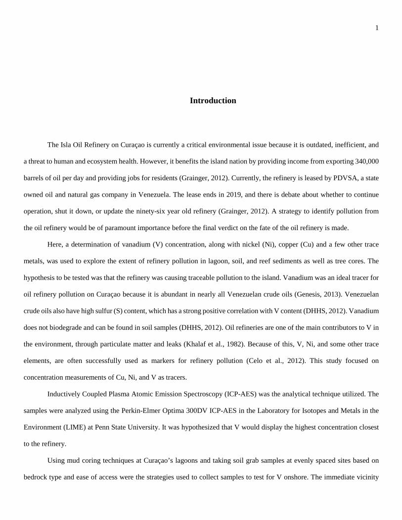
Sample Collection
Samples from Curaçao’s soil, rocks, mud, trees, and sediment were gathered throughout the island to achieve the
goal of tracing potential pollution from the Isla Oil Refinery. The sample types and locations are shown in Figure 1.
Figure 1. Types and Locations of samples gathered on Curaçao in 2014.
Soil
To collect a soil sample, an area was chosen no less than twenty feet away from a roadway or human habitation. A
greater distance away was desired and often available, but sometimes thick underbrush with thorns prevented further travel.
Once a sample location was determined, a shallow hole was dug to remove leaf debris. Without contaminating the sample
by touching the soil, the sample was scooped into a falcon tube.
4
Samples were gathered on each part of the island, paying special attention to the area ringing the oil refinery. The
refinery itself was not available for public access. Figure 1 shows where each sample was taken. A total of eighty nine soil
samples were gathered throughout the island by a team of eleven students who were instructed on proper techniques.
Rocks were also chosen at several locations. The rocks were considered parent material to the residual soil above
them, and thus would provide a standard against which Vanadium concentration was compared (discussed later). The
location of each rock sample is displayed in Figure 1. Five rocks of different parent material were gathered, representing
the major bedrock types on Curaçao.
Sediment
To collect sediment samples from the ocean, snorkel or SCUBA gear was needed. The sampler dove to the ocean
bottom and collected the sediment with a falcon tube. Samples were not touched due to potential contamination. Figure 1
shows the approximate location from which each sample was taken, labeled Sediment Sample. The GPS coordinates mark
the beach nearest to the sampling place, rather than the ocean location, since GPS does not work underwater.
Tree Cores
Cores were extracted from thirteen Haematoxylum Brasiletto trees. This type of tree was chosen because of its
abundance on the island. To obtain a core, the tree corer was twisted by hand into the tree at a point approximately four and
a half feet off the ground. The corer was inserted further until a small clicking or snapping sound was heard. That was the
indication that the corer had been filled with tree matter and had sliced the core to disconnect it from the tree. To extract the
core, the core tube was removed from the tree corer while the corer was still in the tree. The core sample was removed from
the core tube and placed in a plastic bag. The corer could then be removed from the tree by untwisting it. Figure 1 shows
the location of the trees where coring took place. To view a photo of the coring process, see Appendix 3.

5
Before shipping, the tree cores were slid inside a clean plastic drinking straw to prevent breakage. The straw was
taped shut on each end and returned to a plastic bag. Some cracking did occur during transportation. However, the straw
prevented the pieces from becoming disordered.
Mud Cores
A 5cm diameter and 1m length plastic mud coring tube was utilized to obtain mud cores. Mud core sampling
locations were chosen that had up to two feet of water coverage and mud at least eighteen inches deep. To take a mud core,
the caps on each end of the corer were removed, and the corer was pressed through the water and mud. Care was taken not
to block the top of the corer, as this would cause air pressure to build and prevent mud from entering the core. The corer
was pushed into the mud until the top reached the level of the water, and then a hole was dug around the tube to reach the
end farthest in the mud. Once the deep end of the corer was reached, a hand was placed over the end of the core to prevent
the sample from falling out, and the core was removed from the water. Both ends of the core were capped, and the core was
labeled to ensure the top and bottom of the core were not confused with each other. To view one of the mud cores taken at
the site, see Appendix 3.
Sample Preparation
Soil
A portable ashing furnace was used to ash the samples. A similar ashing furnace can be seen in Appendix 3. Each
sample was poured into a crucible and heated to a temperature of 800ºC for an average of two hours in the furnace. Once
ashed, each sample was poured into a glass vial for storage and shipping.
6
To further prepare the soil samples for analysis, a mortar and pestle was used to grind each sample so that the
particle size was below 150 microns, which helps the sample dissolve into a solution prior to entering the ICP-AES
instrument. After grinding, each sample was sieved. Because of different minerals in each sample, some sample aliquots
that did not pass through the sieve needed to be ground multiple times.
To prepare rock samples for analysis, each rock was hammered into smaller pieces. The rocks were wrapped in
paper towels to prevent contamination from the hammer or the metal surface they were pounded against. A mortar and
pestle were then used to further grind down the rocks. Samples were then treated as described for the soil samples.
Sediment
The sediment samples were separated into sand and silt by sieving. Each sample was poured into a 100 micron
sieve, and then water was poured into the sieve to separate the individual particles. The sieve was shaken for 5 minutes by
hand. Silt particles smaller than 100 microns passed through the sieve, leaving the sand particles behind. Once the sand and
silt were separated, the samples were poured into pans and heated on the stove to remove water. The dry samples were then
poured into glass vials for storage and shipping.
To prepare samples for analysis, each sand and silt sample was poured into a shallow aluminum cup and weighed.
The samples were then baked at 50 °C for 48 hours. The sample weights were recorded after 24 hours of baking and once
the baking had completed.
Tree Cores
To prepare tree cores for analysis, they were air dried. This was done by slicing the straws they were stored in to
let moisture evaporate.
7
The cores were then sliced lengthwise using a Leica CM 370 microtome to heighten the clarity of the rings and
prepare a flat core surface for laser ablation. A picture of a similar microtome can be seen in Appendix 3. Effectiveness of
laser ablation is increased when the surface being analyzed is flat rather than rounded.
To use the microtome, each core was sliced into segments between ¾ in and 1 ¼ in long using a razor blade. Each
segment was connected to a metal disc using cryomatrix and placed inside the instrument. Once the cryomatrix froze,
attaching the core firmly to the disc, the disc was placed into the cutting slot and the core was shaved down lengthwise by
approximately one third, revealing the rings and creating a flat core surface. The core segments were then removed from
the instrument, placed in plastic bags, and labeled.
Mud Cores
Each of the five mud cores were extruded from the core tubes and sliced into 1 cm segments. They were labeled
according to their core number and a letter of the alphabet. For example, the label 1A would represent the oldest and deepest
segment of core 1. The labeling scheme and number of segments in each core can be seen in Table 1. The segments were
placed on aluminum foil and air dried at room temperature. After air drying for several days, the segments were weighed.
They were then baked in aluminum cups for 24 hours at 50 °C and weighed again. A final baking session of 24 more hours
was used to remove the remainder of the moisture. After the total 48 hours of baking, the final weight of each mud core
segment was recorded.

8
Table 1. Amount and Labels of Mud Core Segments
Core Number Core Segment Labels Total Number of Segments in Core
1 1A-1V 22
2 2A-2V 22
3 3A-3O (some segments missing) 13
4 4A-4AB 28
5 5A-5S 19
Discrete samples of organic material were taken from some segments of each core and archived for possible
radiocarbon dating at a later date. Types of organics included leaves, stems, tar, and shells. The segments that the organics
were collected from are listed in Table 2.
Table 2. Mud Core Segments with Organic Material Extracted
Core Segment Label
1F
1Q
2B
2I
3A
4A
4N
5B
5M

9
Five samples of each core were chosen for ICP-AES analysis so that a potential trend, if present, could be observed
in the concentration of vanadium and nickel through time and in each core. Thus, not every mud core segment was processed
and analyzed due to time and financial constraints. To prepare the samples, a quarter of each chosen core segment was
ground. The edge that had touched the core tube was scraped away to prevent sample smearing. The remainder was then
ground using a mortar and pestle and sieved to a size below 150 microns. Core segments that were ground for analysis can
be seen in Table 3.
Table 3. Mud Core Samples Chosen for ICP-AES Analysis
Core 1 Core 2 Core 3 Core 4 Core 5
1A 2A 3A 4A 5A
1G 2G 3D 4H 5D
1L 2L 3J 4M 5J
1Q 2Q 3M 4X 5S
1V 2V 3O 4AB 5P
10
Data Analysis
Due to uncontrollable situations, usable data was not gleaned from every sample type. The laser ablation instrument
was under maintenance throughout the data analyzing process, so an elemental analysis on tree cores was not performed.
Laboratory analyses were successfully achieved for all processed soil, mud, and sediment samples. Because there was little
to no clay in the sediment samples taken, the results in that portion of the experiment were inconclusive. Trace metals do
not adsorb to the calcium carbonate sand as well as they do to clay. The soils and mud of Curaçao, though, revealed relevant
information. The remainder of this discussion will focus on the results obtained from those media.
Soil
All of the points from the soil analysis are displayed in Figure 2. The ring of samples in the southwestern part of
the island encircles the refinery. Except for the southernmost tip of the island where there were no roads, samples were
gathered throughout much of the island. Because of the number of samples gathered, the soil analysis is considered to be
the most robust data set for assessing potential refinery-related pollution.

11
Figure 2. Locations of all the Soil Samples.
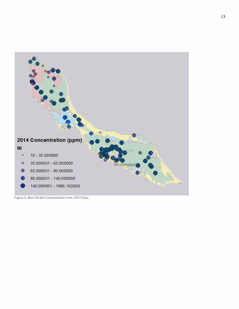
Concentration data for oil pollution tracers Cu, Ni, and V can be seen in Figures 3-5. In the background of each
map is a color coded representation of the geology of Curaçao. Each color indicates a different parent rock material. Red is
for the Knip Group, green for Curaçao Lava Formation, blue for Middle Curaçao Formation, and yellow for Quaternary
Limestone. The data table for the elements can be seen in Appendix D.

12
Figure 3. Raw Copper Concentration from 2014 Data
13
Figure 4. Raw Nickel Concentration from 2014 Data

14
Figure 5. Raw Vanadium Concentration for 2014 data.
From these maps alone, it is difficult to see any existing trend that may indicate pollution. The raw elemental
concentrations must be compared against a baseline of values. One such baseline would be concentration data from an old
study. In 1992, a soil geochemical survey of Curaçao took place, and concentrations of elements including Cu and Ni were
measured in soil throughout the island (de Vries, 2000). If the refinery was responsible for environmental pollution, then
measurable buildup would likely occur over the years. Comparing the 22 year old data maps in Figures 6 and 7 with the
maps in Figures 3 and 4 suggests some interesting relationships.

15
Figure 6. Raw Copper Concentration from 1992 Geological Survey

16
Figure 7. Raw Nickel Concentration from 1992 Geological Survey.
In both maps, there is a marked increase in concentrations of Cu and Ni over the twenty-two year period, especially
in the middle and northern sections of the island. The southern part of the island is where the refinery is located, so the
concentration of pollution tracers would likely show the most increase there. This indeed seems to be the case.
Though Fe was not part of the 2014 study, it is also an oil pollution indicator and was part of the geological survey
of 1992 (de Vries, 2000). In Figure 8, the Fe concentration map shows a similar trend to the maps of Cu and Ni. Though
there are a few spots of high concentration in the northern part of the island, the majority of the Fe is located south, nearer
to the refinery.

17
Figure 8. Raw Iron Concentration from 1992 Geological Survey
To determine whether the concentration of a particular element in the soil is unusually high, the soil’s raw
concentration must be compared to the parent rock concentration. This is done using Equation 1, the tau equation. Tau gives
a value that effectively compares concentration of a mobile element to its concentration in the parent material.
𝑇𝑇𝑇𝑇𝑇𝑇 = (𝐶𝐶𝑚𝑚𝑆𝑆𝑜𝑜𝑜𝑜𝑜𝑜 × 𝐶𝐶𝑜𝑜𝐶𝐶𝑇𝑇𝐶𝐶𝐶𝐶𝐶𝐶𝐶𝐶)/(𝐶𝐶𝑚𝑚𝐶𝐶𝑇𝑇𝐶𝐶𝐶𝐶𝐶𝐶𝐶𝐶 × 𝐶𝐶𝑜𝑜𝐶𝐶𝑜𝑜𝑜𝑜𝑜𝑜) − 1 Equation 1. 𝐶𝐶𝑚𝑚𝑆𝑆𝑜𝑜𝑜𝑜𝑜𝑜 = Concentration of mobile element in soil 𝐶𝐶𝑜𝑜𝐶𝐶𝑇𝑇𝐶𝐶𝐶𝐶𝐶𝐶𝐶𝐶 = Concentration of immobile element in parent rock 𝐶𝐶𝑚𝑚𝐶𝐶𝑇𝑇𝐶𝐶𝐶𝐶𝐶𝐶𝐶𝐶 = Concentration of mobile element in parent rock 𝐶𝐶𝑜𝑜𝐶𝐶𝑜𝑜𝑜𝑜𝑜𝑜 = Concentration of immobile element in soil

18
The immobile element used for the tau equation was Zirconium (Zr). Cu, Ni, and V were the mobile elements. The
mapped results of the tau comparison can be seen in Figures 9-11. The table of tau values for each element and their locations
can be viewed in Appendix E. All negative values were recorded as “0” to maintain a useful data set.
Figure 9. Copper Tau Data 2014

19
Figure 10. Nickel Tau Data 2014

20
Figure 11. Vanadium Tau Data 2014
Most of the samples that display a high elemental concentration in the soil compared to the parent material occurred
close to the refinery. For the Ni and V maps, the southwest portion of the ring around the refinery showed the highest tau
values. This could be due to the southwest trade winds that Curaçao experiences. The winds could potentially blow the
metal as particulate matter from the refinery’s stacks and deposit it in the ocean and southwestern edge of the island.
Looking at the maps as a whole, there appears to be an increase in raw concentration from 1992 to 2014 for both
Ni and Cu. Calculating tau values indicated that compared to the parent material, there was more Ni, V, and Cu around the

21
refinery, especially in the southwestern portion. These results could indicate that the refinery has polluted Curaçao’s soil
environment.
Mud Cores
The location of the five mud cores gathered from the island can be seen in Figure 12. Though the number of cores
was few, they were spaced widely throughout the island for a more accurate description of the island’s metal concentration
in lagoonal mud. The sedimentation rate for each core was estimated by using a value from literature and relative
sedimentation rates between cores (Klosowska et all, 2004). The details of this strategy are discussed below. This helped to
formulate an idea of what core depth corresponded to what year. Each rate is displayed in Figure 12 next to the core number.
Figure 12. Locations of Mud Cores and Estimated Sedimentation Rates
Using ICP-AES analysis, concentrations of Ni and V were calculated for five segments of each core (see Table 3)

22
to observe varying concentration trends throughout the island’s history and potentially ascertain evidence of refinery impact.
Concentrations of other elements and compounds, Cu, Cr, Zn, Zr, and Al2O3 were calculated to normalize the raw element
concentrations and assist in determining the core’s timeline.
The concentration of elements was normalized by dividing by the concentration by Al2O3, which adjusts for
variations in clay content. Though organic pieces of each core were taken, there was a lack of time and resources to carbon
date them. Instead, to estimate the timeline of the cores, the depth of the Cr and/or Cu peak was assumed to occur at a similar
time for all cores because of a spike in input. By comparing the depth of these peaks, a timeline of the cores relative to each
other could be created.
The sedimentation rate in a lagoon in Curaçao (Klosowska et al, 2007) was found to average 1.65 mm/year.6 Our
Core 5 was taken from the same lagoon, so the sedimentation rates were assumed to be the same or similar. Approximate
absolute time lines for each core were then constructed using the literature value and the relative time lines between cores.
These sedimentation rates are displayed in Figure 12.
The timeline was constructed under the assumption that the elemental peaks occurred at the same moment in time.
If that was not the case, the results would differ. However, the sedimentation rates obtained can be rationalized. Core 3 and
4 at the southernmost part of the island would be expected to have similar sedimentation rates not only because of their
proximity, but they also both had mangroves - small salt water habitat trees - near their lagoons and the outlet to the sea.
This can be seen in the close up map in Figure 13.7 Mangroves, with their complex root system, contribute to erosion
prevention, so an area with mangroves would have a higher sedimentation rate than an area without because the accumulated
sediment would not be washed away. This is indeed reflected in the calculated sedimentation rates.

23
Figure 13. Closeup Map of Core 3 and 4 Lagoons7
Core 3 was shorter than the other cores, so the depth of the Cr/Cu peak was not revealed. It had to be estimated
based on the concentration of Cr at the deepest point and at what depth/time the peak existed in other cores after reaching a
similar concentration. The five graphs of how the normalized elemental concentrations varied with time can be seen in
Figures 14-18.

24
Figure 14. Core 1 vs. Time with Al2O3 Normalized Concentrations

25
Figure 15. Core 2 vs. Time with Al2O3 Normalized Concentrations

26
Figure 16. Core 3 vs. Time with Al2O3 Normalized Concentrations

27
Figure 17. Core 4 vs. Time with Al2O3 Normalized Concentrations
28
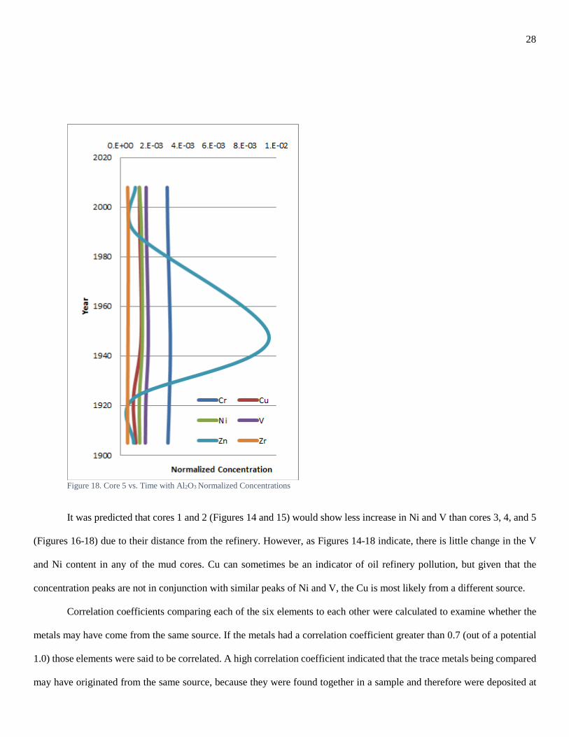
Figure 18. Core 5 vs. Time with Al2O3 Normalized Concentrations
It was predicted that cores 1 and 2 (Figures 14 and 15) would show less increase in Ni and V than cores 3, 4, and 5
(Figures 16-18) due to their distance from the refinery. However, as Figures 14-18 indicate, there is little change in the V
and Ni content in any of the mud cores. Cu can sometimes be an indicator of oil refinery pollution, but given that the
concentration peaks are not in conjunction with similar peaks of Ni and V, the Cu is most likely from a different source.
Correlation coefficients comparing each of the six elements to each other were calculated to examine whether the
metals may have come from the same source. If the metals had a correlation coefficient greater than 0.7 (out of a potential
1.0) those elements were said to be correlated. A high correlation coefficient indicated that the trace metals being compared
may have originated from the same source, because they were found together in a sample and therefore were deposited at

29
approximately the same time. Tables 4-8 show the correlation coefficients of the six trace elements examined in the mud
cores, normalized to Al2O3. The elements that correlated were highlighted.
Table 4. Core 1 Correlation Coefficients
Cr ratio Cu ratio Ni ratio V ratio Zn ratio Zr ratio Cr ratio 1 Cu ratio -0.87993 1 Ni ratio -0.65158 0.85984 1 V ratio -0.20341 -0.09088 -0.52339 1 Zn ratio -0.73839 0.383436 0.017658 0.761077 1 Zr ratio 0.098361 0.207546 0.570495 -0.97974 -0.71177 1
Table 5. Core 2 Correlation Coefficients
Cr ratio Cu ratio Ni ratio V ratio Zn ratio Zr ratio Cr ratio 1 Cu ratio 0.952089 1 Ni ratio -0.96917 -0.9629 1 V ratio -0.88191 -0.75052 0.864466 1 Zn ratio -0.81675 -0.61048 0.721847 0.828259 1
Zr ratio 0.84944 0.748234 -0.89284 -0.96194 -0.77489 1
Table 6. Core 3 Correlation Coefficients
Cr ratio Cu ratio Ni ratio V ratio Zn ratio Zr ratio Cr ratio 1 Cu ratio 0.33139 1 Ni ratio 0.224454 0.991528 1 V ratio 0.75395 -0.24542 -0.31652 1 Zn ratio 0.944335 0.242445 0.160782 0.852166 1 Zr ratio 0.016442 0.858295 0.887493 -0.50545 -0.00029 1

30
Table 7. Core 4 Correlation Coefficients
Cr ratio Cu ratio Ni ratio V ratio Zn ratio Zr ratio Cr ratio 1 Cu ratio -0.31026 1 Ni ratio 0.70218 0.21767 1 V ratio 0.4671 0.613974 0.531542 1 Zn ratio 0.289144 -0.09446 -0.14675 0.489772 1 Zr ratio 0.044649 0.917971 0.428633 0.871348 0.188492 1
Table 8. Core 5 Correlation Coefficients
Cr ratio Cu ratio Ni ratio V ratio Zn ratio Zr ratio Cr ratio 1 Cu ratio -0.01699 1 Ni ratio 0.525939 0.735135 1 V ratio 0.694762 0.69506 0.856845 1 Zn ratio 0.775501 0.566924 0.786263 0.938173 1 Zr ratio 0.104565 0.668293 0.82733 0.522531 0.317094 1
Looking only at the number of highlighted values, it would seem that there may be significance in the correlating
elements. However, instead of making that assumption, a p-value was calculated for each of the highly correlating metals.
If the p-value was smaller than 0.05, it indicated that the null hypothesis (no relationship until proven otherwise) could be
rejected with 95% confidence. Only 38% of the highly correlated metals had a p-value <0.05. Figures depicting the highly
correlated elements with p-values <0.05 can be viewed in Appendix B. Of those few, there was no significant relationship
between the metals in each core that were correlated.
These results from the concentration vs time plots and the correlation calculations indicate that:
1. The mud in the tested lagoons does not reflect any definitive change in pollution from refinery activity throughout
the course of the refinery’s existence.
2. The pollution indicator metals were not deposited in a revealing pattern together through time.
Neither of these results, however, means that pollution does not exist. Wind or ocean outlets may have contributed
to sweeping away the trace metal indicators before they drifted to the mud. Other lagoons not sampled may reflect different
results. Perhaps if permission was granted for mud closer to the refinery to be analyzed, a different picture would emerge.

31
Sample collecting any closer was prohibited because of fencing that kept the area around the refinery off limits to civilians,
however. Also, only five 1 cm long samples from each core were analyzed through ICP-AES. This limitation in the number
of samples, due to time and resource constraints, makes the mud core analysis much less accurate than the soil analysis,
which had nearly 200 analyzed samples. If more samples were analyzed, a more complete picture of the island’s pollution
history might be revealed.

32
Conclusion
Trace elements such as V, Ni, and Cu, were used to trace potential pollution from the Isla Oil Refinery on Curaçao.
Both soil sample and mud core data must be taken into consideration before concluding whether or not there is refinery
pollution in the terrestrial environment of the island. The soil data maps shown in Figures 3, 4, 6, and 7 indicate that the
concentration of Ni and Cu both increased between 1992 and 2014. Calculating tau values of elements in the soil showed
that compared to the parent rock material, there was more Ni, V, and Cu close to the refinery than in other areas of the
island. These results indicate that soil pollution from the refinery is a likely possibility.
The mud core results were more difficult to interpret than the soil data. There were far fewer cores than soil samples
(five cores compared to almost 200 soil samples), and only five segments of each core were analyzed by ICP-AES.
Nevertheless, the time lines constructed for each core did not indicate any significant increases in Ni or V over the course
of the refinery’s life for any of the locations. There were some significant Cu peaks, but since Cu does not increase in
conjunction with Ni or V, the input most likely does not originate from the refinery. There was also no significant pattern
in the correlation between the trace metals in each core. These results do not necessarily mean that the refinery is not
polluting the mud. Taking more cores and analyzing more samples from each core would give a more accurate picture of
the island’s elemental history.
Overall, there is a real possibility that the Isla Oil Refinery is significantly impacting Curaçao’s terrestrial
environment. More data and more varieties of data would need to be analyzed for this proposition to be conclusive, though.
Analyzing the tree cores, additional mud cores, a greater number of sediment samples, and possibly collecting air samples
would all be beneficial next steps to continue the investigation.

33
Appendix A
Contact List for Experiment
Table 9. Contact List for Experiment
First Name Last Name Email
Coriana
Elizabeth
Fitz
Andrews
Rochelle
Lissie
Linsenbigler
Poyner
Anton
Bobby
Everleigh
Jenna
Madeline
Josh
Marissa
Paton
Reynolds
Stokes
Thomas
Muto
Turner
Defratti

34
Appendix B
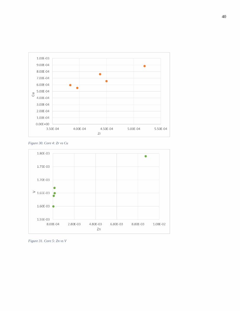
Mud Core Correlation Coefficient Figures
All figures plot the normalized concentration (ppm) of one trace metal against another trace metal. Based on these
values, correlation coefficients were calculated for each element pair in each core. The coefficients themselves can be
viewed in Tables 4-8 in the analysis.
Figure 19. Core 1: Cu vs Cr

35
Figure 20. Core 1: Zr vs V
Figure 21. Core 2: Cu vs Cr

36
Figure 22. Core 2: Ni vs Cu
Figure 23. Core 2: Zr vs V

37
Figure 24. Core 2: Ni vs Cr
Figure 25. Core 2: V vs Cr

38
Figure 26. Core 2: Zr vs Ni
Figure 27. Core 3: Ni vs Cu

39
Figure 28. Core 3: Zn vs Cr
Figure 29. Core 3: Zr vs Ni
40
Figure 30. Core 4: Zr vs Cu
Figure 31. Core 5: Zn vs V

41
Appendix C
Tools and Instruments
Figure 32. Tree Coring in Curaçao
Figure 33. Mud Core Collected on Curaçao
Figure 34. ICP Atomic Emission Spectromoter (American Assay 2015)

42
Figure 35. LEICA Microtome (ASU 2015)
Figure 36. Portable Ashing Furnace (NACAAF 2015)

43
Appendix D
Concentration and Location Data for Elements
Table 10. 2014 Concentration and Location Data for Soil Samples
V (ppm) Cu (ppm) Ni (ppm) Latitude (°) Longitude (°) 312.342 125.4499 86.79105 12.35293 -69.1465 150.381 75.8916 24.66825 12.33915 -69.1469 238.357 161.2862 337.5762 12.29482 -69.1264 236.539 122.8259 221.7198 12.28003 -69.1153 311.229 163.3056 119.7579 12.24675 -69.0628 256.807 129.9642 148.6959 12.3238 -69.1513 97.337 102.7143 83.1385 12.34457 -69.1419
316.790 134.6441 102.1909 12.37242 -69.137 45.501 76.60535 71.70985 12.34927 -69.1061
260.480 94.1103 126.6793 12.33217 -69.0913 308.310 213.1547 62.8391 12.31195 -69.0909 368.192 161.6204 100.7004 12.29622 -69.098 163.816 91.3059 125.7206 12.22937 -69.0339 182.007 103.6685 80.1903 12.2033 -69.0136 209.511 102.5745 301.3225 12.27346 -69.0664 202.534 117.3372 286.8936 12.09021 -68.8237 235.872 104.3554 253.1755 12.10541 -68.8405 212.668 138.5634 131.8299 12.11473 -68.8322 243.316 116.3055 263.0713 12.13808 -68.9379 180.681 113.7252 218.9547 12.07226 -68.8127 289.923 172.3757 207.1162 12.0931 -68.861 371.094 125.0656 224.6074 12.13038 -68.9496 278.275 147.6733 221.5834 12.13408 -68.9504 299.949 168.7727 185.7799 12.13642 -68.9473 445.501 310.3544 366.0675 12.1367 -68.9417 230.037 219.8314 149.7323 12.12028 -68.9097 182.212 259.8841 104.8256 12.11202 -68.9116 201.029 93.29675 293.2971 12.10738 -68.9206 186.372 173.5857 141.2106 12.11398 -68.9297 128.690 60.0965 172.9174 12.11528 -68.9448 229.307 102.5787 234.0329 12.11997 -68.9474 389.295 154.6464 305.1385 12.1252 -68.9561 231.741 120.4812 234.5774 12.12272 -68.9563 579.233 94.90805 265.6943 12.12283 -68.9564 312.933 155.2922 243.2473 12.13582 -68.9511 211.344 149.2878 255.9136 12.15943 -68.9718 251.255 139.2898 185.6886 12.12803 -68.8976 269.854 149.23 150.6592 12.16098 -68.9442 29.707 37.31945 27.782 12.18353 -68.9643
189.018 72.56155 138.8277 12.18112 -68.989 197.118 121.6718 151.9162 12.16 -68.99

44
57.863 41.32985 30.8995 12.30687 -69.1446
162.392 71.3481 78.62455 12.12743 -68.825 113.047 64.1997 126.8342 12.07338 -68.8614 214.388 461.3863 70.19812 12.27202 -69.1228 76.987 98.925 54.02815 12.35192 -69.114 89.437 2023.379 49.8262 12.33573 -69.1073 29.332 16247.76 216.337 12.32046 -69.1489
214.766 154.1215 356.7707 12.35211 -69.0805 324.872 184.2195 249.0319 12.32032 -69.1483 342.655 158.7675 1986.163 12.264 -69.091 -1.308 18.3775 27.2738 12.318 -69.151
332.313 170.029 73.6661 12.214 -69.055 8.554 46.8595 20.81645 12.119 -68.96
82.431 67.817 35.86755 12.3364 -69.1474 108.476 109.631 23.1111 12.35093 -69.1451 296.862 140.5875 150.1305 12.30692 -69.1386 137.703 72.0085 81.5157 12.26935 -69.098 178.823 84.6335 86.63785 12.33985 -69.1553 254.503 153.869 111.3653 12.38647 -69.146 325.976 153.9195 103.1521 12.37793 -69.1563 115.993 86.9565 47.7503 12.36752 -69.1219 175.555 70.544 141.9852 12.22503 -69.0607 168.446 84.5325 97.02185 12.21292 -69.0514 192.466 80.9975 132.7918 12.20692 -69.0197 219.085 80.139 143.3357 12.20692 -69.0197 319.635 194.976 132.7605 12.19942 -69.0504 322.856 157.1515 148.4429 12.21922 -69.0231 177.249 100.339 104.1874 12.2502 -69.0564 188.446 73.271 196.8443 12.27262 -69.0721 275.611 142.153 104.002 12.28905 -69.0721 216.821 119.8825 212.5821 12.09418 -68.827 300.352 142.052 233.8814 12.13783 -68.961 356.398 123.973 264.5859 12.12587 -68.9627 241.212 147.001 212.6229 12.11853 -68.9617 134.573 88.3705 84.16295 12.10873 -68.9502 199.742 157.707 238.0394 12.12303 -68.9487 294.074 137.709 287.1041 12.12595 -68.9489 223.992 196.1375 147.5334 12.13982 -68.933 264.880 206.0355 177.0936 12.14357 -68.926 196.956 172.756 146.1304 12.14375 -68.921 202.897 125.0335 138.7729 12.13778 -68.9183 225.018 153.9195 167.665 12.13635 -68.9127 231.768 347.1325 199.8146 12.13147 -68.9088 235.542 129.6795 203.0854 12.12732 -68.8261 312.228 188.007 78.66295 12.12753 -68.8546 216.229 119.2765 305.6798 12.10728 -68.9035 184.611 131.548 120.734 12.17552 -68.872 241.235 169.2715 217.6719 12.1561 -68.9056 250.111 141.2945 180.0652 12.14525 -68.9318 316.550 119.226 320.3353 12.35469 -69.0941

45
Appendix E
Tau and Location Data for Elements
Table 11. 2014 Tau Values and Locations for Soil Samples
Nitau Vtau Cutau Latitude (°) Longitude (°)
0 0 3.5008 12.33573 -69.1073
0 0 0 12.35211 -69.0805
0 0 0 12.3069 -69.1386
0 0 0.008 12.29481 -69.1265
0 0 0 12.28004 -69.1153
0 0 0 12.26939 -69.098
0 0 0 12.24691 -69.0627
0 1.383 0 12.38987 -69.1553
0 0 0 12.38646 -69.146
0 0 0 12.37794 -69.1563
0 0 0 12.37241 -69.137
0 0 0 12.36749 -69.1219
0 0 0 12.29626 -69.0978
0 0 0 12.22504 -69.0607
1324.179 0 0 12.30305 -69.1192
0 0 0 12.20686 -69.0197
918.745 0 0 12.20585 -69.0244
0 0 1.124 12.19942 -69.0504
0 0 0 12.22936 -69.0339
0.815 0 0 12.21906 -69.0229
0 0 0 12.20297 -69.0139
0.045 0 0 12.2502 -69.0564
0.369 2.189 0 12.27265 -69.0535
0.148 6.406 0 12.28921 -69.0722
0.435 0 0 12.0942 -68.827
0 0 0 12.27346 -69.0664
0.904 0 0 12.09021 -68.8237
0.571 0 0 12.10541 -68.8405
0 0 0 12.11473 -68.8322
0.516 0 0 12.13808 -68.9379
0.356 0 0 12.07226 -68.8127
0.292 0 0.063 12.0931 -68.861

46
0.684 0.125 0.011 12.13782 -68.961
1.035 0.426 0 12.12588 -68.9627
1.322 5.411 0 12.11855 -68.9616
0.311 55083.43 1.043 12.1087 -68.9502
1.02 0 0.323 12.12303 -68.9487
1.219 0.182 0.052 12.12601 -68.9489
0.392 0.196 0 12.13043 -68.9496
0.33 0 0 12.13409 -68.9503
0.191 0 0.069 12.13641 -68.9473
0.695 0.073 0.421 12.13671 -68.9417
0.099 0 0.444 12.1398 -68.933
0.113 0 0.28 12.14359 -68.9259
0 0 0.016 12.14374 -68.921
0.164 0 0.037 12.13778 -68.9183
0.244 0 0.129 12.13636 -68.9127
0.429 0 1.454 12.13148 -68.9088
0 0 0.388 12.12029 -68.9097
0.116 3.721 0.229 12.11201 -68.9116
1.277 0 0 12.10738 -68.9206
0.628 4.229 0 12.11397 -68.9297
1.239 3.054 0 12.11529 -68.9448
0.738 0 0 12.11999 -68.9474
0.859 0.233 0 12.12522 -68.9561
0.618 0 0 12.12271 -68.9563
0.129 0.279 0 12.12284 -68.9564
0.506 0.007 0 12.13582 -68.9511
0.609 0 0 12.15941 -68.9719
0.239 0 0 12.1273 -68.8261
0 0 0.04 12.12759 -68.8546
1.192 0 0 12.10729 -68.9035
0.087 0 0 12.12802 -68.8974
0 1.96 0 12.17555 -68.872
0.361 0 0.046 12.15616 -68.9056
0.143 0 0 12.14705 -68.928
0 0 0 12.14528 -68.9318
0 0 0 12.16116 -68.945
0 0 0 12.18374 -68.9643
2.5954 0 0 12.1815 -68.989

47
BIBLIOGRAPHY
1. American Assay Laboratories, 2015, Atomic Emission Spectrometry, web. http://www.aallabs.com/technology/icp-aes
2. ASU Knowledge Enterprise Development, 2015, Leica CM 1950 Cryostat, web.
http://sharedresources.asu.edu/resources/5066
3. Celo, Valbona, Dabek–Zlotorzynska , Ewa, Zhao, Jiujiang, Bowman, David, 2012, Concentration and source origin of
lanthanoids in the Canadian atmospheric particulate matter: a case study, Atmosphere Pollution Research, pg. 270-278.
http://www.atmospolres.com/articles/Volume3/issue3/APR-12-030.pdf
4. de Vries, A.J., 2000, The Semi-arid Environment of Curaçao: a Geochemical Survey, Netherlands Journal of
Geosciences, Vol 79, Issue 4, pg. 479-494.
5. Ellsworth, Brian, 2008, Curaçao Refinery Sputters on, Despite Emissions, Reuters, Web article.
http://www.reuters.com/article/2008/07/01/us-energy-curacao-idUSN2929170620080701
6. Genesis Group, 2013, Venezuela Oil Specifications, Web. http://www.genesisny.net/Commodity/Oil/OSpecs.html
7. Grainger, Sarah, 2012, Carribean island Curaçao faces oil refinery dilemma, BBC News, Curaço, Web.
http://www.bbc.com/news/world-latin-america-17290626
8. Khalaf F., Literathy P., Anderlini V., 1982, Vanadium as a tracer of oil pollution in the sediments of Kuwait,
Developments in Hydrobiology, Volume 9, Abstract. http://link.springer.com/chapter/10.1007%2F978-94-009-8009-9_14

48
9. Klosowska, B. B., Troelstra, S. R., van Hinte, J. E., Beets, D., & van der Borg, K., 2004, Late Holocene environmental
reconstruction of St. Michiel saline lagoon, Curaçao (Dutch Antilles). Radiocarbon, Vol 46, No 2.
10. Nadal, M. Schuhmacher, M. Domingo, J.L., 2003, Metal Pollution of Soils and Vegetation in an Area with
Petrochemical Industry, Elsevier, Science of the Total Environment, Vol 321, Issues 1-3, pg. 59-69.
http://www.sciencedirect.com/science/article/pii/S0048969703005023
11. National Analytical Corporation, 2015, Ashing Chamber Furnaces, 1450, web. http://www.nationalanalyticalcorp.com/ashing-
chamber-furnaces.html
12. Pors , Leendert P. J. J., Nagelkerken, Ivan A.1997, Curaçao, Netherlands Antilles, Unesco, Coastal Regions and Small
Islands Publications, Web article. http://www.unesco.org/csi/pub/papers/pors.htm
13. US Department of Health and Human Services, 2012, Toxological Profile for Vanadium,Ch. 6, pg 121-153.
http://www.atsdr.cdc.gov/toxprofiles/tp58-c6.pdf

49
ACADEMIC VITA
Coriana Fitz [email protected]
________________________________________
EDUCATION The Pennsylvania State University, Schreyer Honors College Expected Graduation Date December 2015 Bachelor of Science in Energy and Mineral Engineering Minor in Environmental Engineering Dean’s list 8/9 semesters
EMS CAUSE 2014 Research class and Curaçao trip (2014) Conducted research, sample collection, preparation, analysis, and discussion on Isla Oil Refinery’s
potential anthropogenic impact on the island of Curaçao. GREEN Program, Costa Rica (2013) Visited solar, geothermal, wind, hydro, and biomass renewable energy plants Installed rainwater collection system on local home Worked on a renewable energy research project. WORK EXPERIENCE
Science-U Program Assistant, Penn State University (2015) Mentored kids ages 6-17 through curriculum in Science-U camps Prepared science experiments for camps Prepared supplies for each new camp week
Microbiology Lab Assistant, Penn State University (2015) Determined Minimum Inoculation Concentration of antifungal compounds Identified synergism of commercial antifungals with boron compounds Monitored growth of various fungi
Teaching Assistant for EGEE 101 and EGEE 102, Penn State University (2013-15) Corrected student homework and answer student questions
Arcade Manager at Valley Worlds of Fun (2014) Monitored games to ensure proper function
Summer Intern at Core Tech, an engineering service firm in New York (2013) Constructed mock-up of pipe connection prototype and tested Communicated with parts manufacturers Wrote technical documents
Summer Internship at NASA Independent Verification & Validation Facility (2011) Global Precipitation Measurement Project Identified faults in the launch and initial processes sequence

50
VOLUNTEER ACTIVITIES Centre County PAWS Volunteer (2015) Penn State University Catholic Campus Ministry Mass Lector (2012-
2015) Penn State University Mission Mexico Trip to Casa Hogar de los
Ninos Orphanage (2011) St. Mary’s Parish Vacation Bible School Teacher (2007-2011) Teen Leadership Camp Counselor (2011-2012)
EXTRACURRICULAR ACTIVITIES Penn State Newman Catholic Club (2011-2015) Licensed recreational SCUBA diver (2014) Penn State Archery Club (2012) Penn State Aikido Club (2011) Reading, Writing, Hiking, Biking, Running, Swimming