School of InformationUniversity of Michigan

SI 614Network visualization (& leftovers from last week)

Lecture 3

Instructor: Lada Adamic

Practical issues

auditing and wanting access to cTools email me so I can add you

cTools usability are there any problems? helpful content?

Pajek any difficulties? discussion threads on cTools

Reading: The structure and function of complex networks by Mark Newman Will be denoted by MEJN followed by a section # or letter

Perl class for SI students (4 Saturday afternoons) The sign up sheet has been posted on the bulletin board outside of the

PEP office, room 406 in West Hall.

Outline

Network sampling Clustering coefficients Question from last time: how web links are stored

Visualization General tips for effective visualizations Visualizing networks

layout algorithms options for large networks longitudinal data visualization software besides Pajek & GUESS

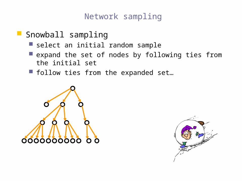
Network sampling

Snowball sampling select an initial random sample expand the set of nodes by following ties from the initial set follow ties from the expanded set…

Network sampling pros and cons

Advantages Finding ‘hidden’ populations

young, male, unemployed cocaine users people with HIV

Well suited for interview-based qualitative research Appropriate where trust is needed to initiate contact

Disadvantages Bias

sample could be biased toward initial set the nodes you are referred to may not be ‘typical’ in connectivity

Inaccurate referrals Difficulty in assuring confidentiality

Snowball sampling and connectivity bias

Probability that you encounter a node with k links is proportional to k

Snowball sampling encounters ‘popular’ nodes more often than unpopular ones

Sampling the internet

Using traceroute to map connections between routers

Accuracy increases as we add more starting points

*Massive deployment: www.tracerouteathome.net ; netdimes.org

source

target

underlying networkderived network:

two sources, two targets

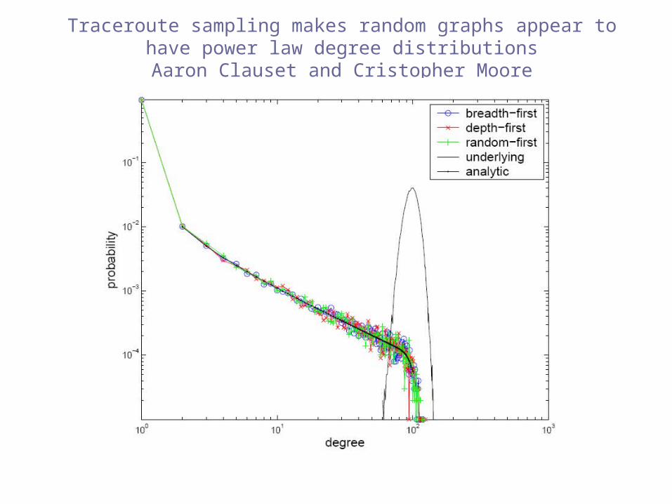
Traceroute sampling makes random graphs appear to have power law degree distributions

Aaron Clauset and Cristopher Moore

How are web links stored efficiently by search engines

From Broder et al, ‘Graph structure of the Web’ Constructed a ‘connectivity server 2’ (CS 2) In CS2, an average of only 3.4 bytes are used per URL database is stored in memory.  On a 465 MHz Compaq AlphaServer 4100, a BFS

reaches 100M nodes in 4 minutes CS2 was built from a crawl performed at AltaVista in

May, 1999. The CS2 database contains 203 million URLs and 1466

million links (all of which fit in 9.5 GB of storage). 

Compressing the web graph

From: Efficient and Simple Encodings of the Web GraphGuillaume et al.

Each URL is assigned a numerical identifier The nth line contains the identifiers of outbound links of

the nth URL Lines are compressed and only the relevant block is

uncompressed to read the links for the nth URL Various other optimizations…

Clustering

Transitivity: if A is connected to B and B is connected to C

what is the probability that A is connected to C?

my friends’ friends are likely to be my friends

Global clustering coefficient3 x number of triangles in the graph

number of connected triples of verticesC =

A

B

C?

Local clustering coefficient (Watts&Strogatz 1998)

For a vertex i The fraction pairs of neighbors of the node that are themselves

connected Let ni be the number of neighbors of vertex i

number of connections between i’s neighbors

maximum number of possible connections between i’s neighbors

# directed connections between i’s neighbors

ni * (ni -1)

# undirected connections between i’s neighbors

ni * (ni -1)/2

Ci =

Ci directed =

Ci undirected =

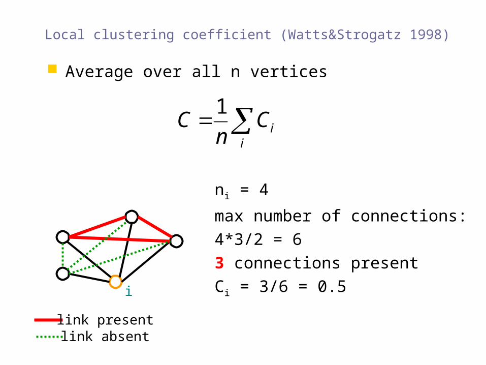
Local clustering coefficient (Watts&Strogatz 1998)

Average over all n vertices

i

iCnC

1

i

ni = 4

max number of connections:

4*3/2 = 6

3 connections present

Ci = 3/6 = 0.5

link absentlink present

John W Tukey

coined word softwarecoined expression exploratory data analysiscoined expression Better to have an approximate answer to the right question than a precise answer to the wrong question

slide: Mick McQuaid

Tufte’s first book popularized many of Tukey’s ideas, especially in the public policy realm

slide: Mick McQuaid

Tips for effective visualizations

"The success of a visualization is based on deep knowledge and care about the substance, and the quality, relevance and integrity of the content.“

(Tufte, 1983) know thy network!

Five Principles in the Theory of Graphic Display Above all else show the data. Maximize the data-ink ratio, within reason. Erase non-data ink, within reason. Erase redundant data-ink. Revise and edit.

Aesthetic criteria for network visualizations

minimize edge crossings

uniform edge lengths (connected nodes close together but not too close)

don’t allow nodes to overlap with edges that are not incident on them

better than

better than

better than

Cool looking visualizations are not always most informative

slide adapted from Katy Borner

http://ridge.icu.ac.jp/gen-ed/ecosystem-jpgs/food-web.jpg http://news.bbc.co.uk/2/hi/science/nature/2288621.stm

Viewing a subset of the network and highlighting node attributes through shape and color enhances understanding

slide adapted from Katy Borner

An Attraction Network in a Fourth Grade Class (Moreno, ‘Who shall survive?’, 1934).

Alden Klovdahl: The core (n~ 450) of a social network of over 5,000 urban residents in Canberra, Australia

Overlaying a network on geographical context

byte traffic into the ANS/NSFnet T3 backbone for the month of November, 1993. Cox & Patterson http://www.caida.org/tools/visualization/walrus/gallery1/

Walrus images of Skitter internet mapping data

Walrus is available under GPL

Longitudinal comparison

Circular layout Circular layout

IPv4 internet graph

AS-level internet map

copyright UC Regents 2004

What counts in a network visualization

Use of color Internet nodes were colored by outdegree Edges colored by degree of endpoints

Use of meaningful coordinates Polar coordinates

r – nodes with higher degree closer in throws leaf nodes toward the outer edge of the graph

or distance from the most central node position along ring denotes geographical latitude

Use of different sizes nodes sized by degree

What else is left? node shape edge thickness

Random Layout

Choose x & y coordinates at random advantage: very fast disadvantage: impossible to

interpret

layout in GUESS

Layout nodes along a circle and draw in all edges between them

Advantages Circular coordinates can

represent a property of the data (e.g. latitude or ‘age’)

Very fast Disadvantages

difficult to interpret for large networks

many overlapping edges many long edges (connected

nodes need not be close together)

clusters hard to identify

Circular layout

layout in GUESS

Circular layout in GUESS

circleLayout(edge_weight, center_node)

image: Andrea Wigginshttp://www-personal.si.umich.edu/~akwiggin/research.html

Place all nodes on a circle

Place center node in the middle

Place center node’s neighbors in a circle around at a radius depending on the weight of the edge

Radial Layout

Start with one node, draw all other nodes in circular layers according to how many hops it takes to reach them

Fast, but no optimization for nodes that are connected to be close together within a layer

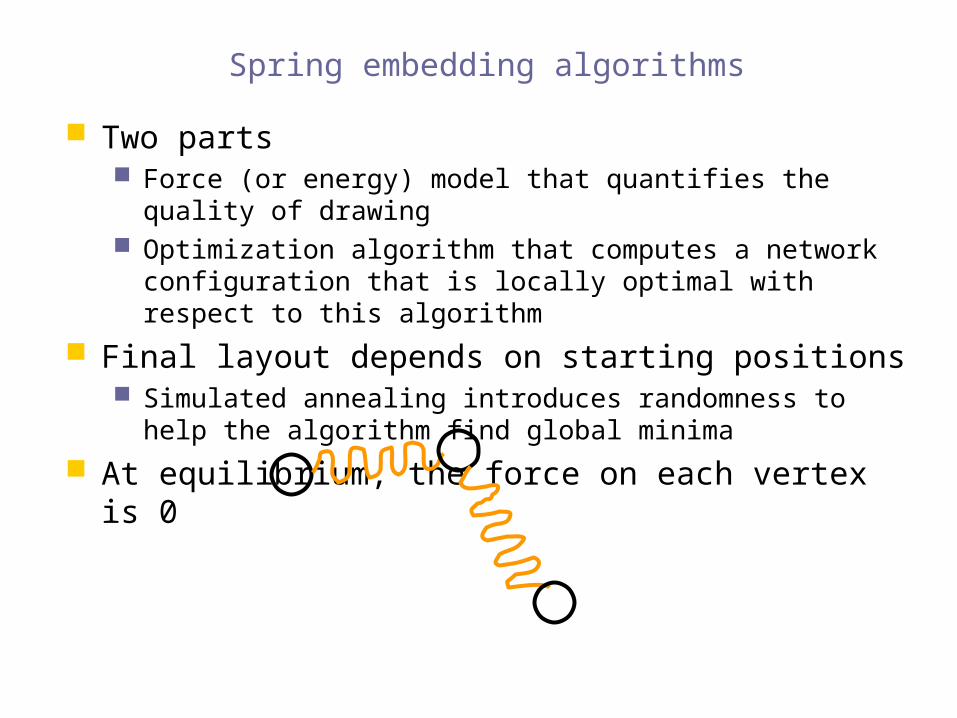
Spring embedding algorithms

Two parts Force (or energy) model that quantifies the quality of drawing Optimization algorithm that computes a network configuration

that is locally optimal with respect to this algorithm

Final layout depends on starting positions Simulated annealing introduces randomness to help the

algorithm find global minima

At equilibrium, the force on each vertex is 0

“manual” spring layouts

Grant's Drawing of a Target Sociogram of a First Grade Class (from Northway, 1952).

McKenzie's Target Sociogram Board (from Northway, 1952).

Pegs and rubber bands used to determine an individual’s location in the sociogram.

computerized spring layouts

Iterative procedure At each time step, allow springs to expand or contract

toward a neutral position

select optimal edge length (node distance) k

repeat

for each node v do

for each pair of nodes (u, v)

compute repulsive force fr(u,v) = - c•

for each edge e = (u,v)

compute attractive force fa(u,v) = c•

sum all force vectors F(v) = ∑ fr(u,v) + ∑ fa(u,v)

move node v according to F(v)

until DONE

Spring layout algorithms: Fruchterman and Reingold

Model roughly corresponds to electrostatic attraction between connected nodes

Use adjacency matrix directly Iterative optimization

at each step, every node reacts to the pulls and pushes of the springs that tie it to all the other nodes

Can be slow as the network grows

layout in GUESS

Spring layout algorithms: Kamada Kawai

All nodes are connected by springs with a resting length proportional to the length of the shortest path between them

Need to calculate all pairs shortest paths first

Iterative optimization Advantage: can be used on

edge- weighted graphs Can be slow as the network

grows

layout in GUESS

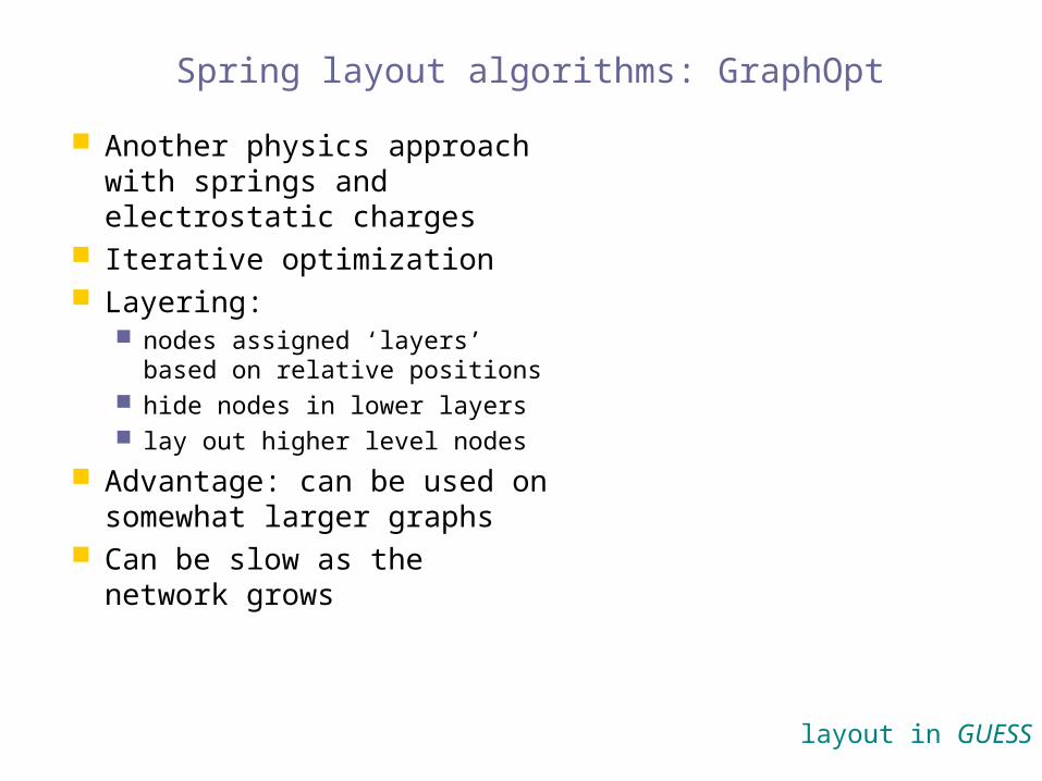
Spring layout algorithms: GraphOpt

layout in GUESS

Another physics approach with springs and electrostatic charges

Iterative optimization Layering:

nodes assigned ‘layers’ based on relative positions

hide nodes in lower layers lay out higher level nodes

Advantage: can be used on somewhat larger graphs

Can be slow as the network grows

There are many variations on spring layout algorithms…

Spring() layout in GUESS

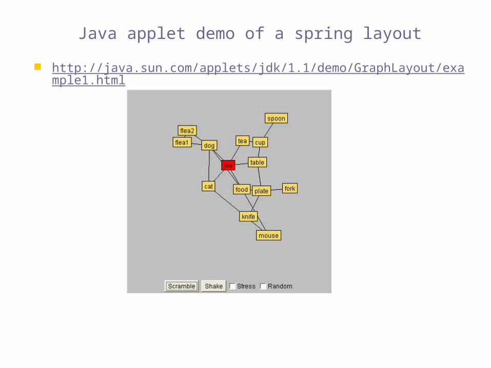
Java applet demo of a spring layout

http://java.sun.com/applets/jdk/1.1/demo/GraphLayout/example1.html

Network layout by gravity

after: Lothar Krempel

unweighted edges weighted edges

locations of blue nodes are fixed

red node experiences gravitational pull from the blue nodes

GEM (graph embedding) Layout

Embedding algorithm with speed & layout optimizations Significantly faster than KK or FR In GUESS, you can lay out 1,000 – 10,000 node graphs,

depending on the edge density

layout in GUESS

Multidimensional scaling concept

Metric MDS gives an exact solution based on a Singular Value Decomposition of the input matrix.

Input matrix can be the all pairs shortest path or another ‘distance matrix’

Usually the data is plotted according to the eigenvectors corresponding to the two largest eigenvalues

Multidimensional scaling

using random edge weights rather than average shortest paths

layout in GUESS

Strategies for visualizing large graphs

Reduce the number of nodes and edges introduce thresholds

only authors who have written at least x papers only edges with weight > y only nodes with degree > z (e.g. removing leaf nodes)

show minimum spanning trees can visualize all the nodes with a subset of the edges

use pathfinder network scaling (http://iv.slis.indiana.edu/sw/pfnet.html) triangle inequality to eliminate redundant or counter-intuitive links remaining edges are more representative of internode relationships

than minimum spanning trees collapse nodes into clusters

show multiple nodes as a single node display connections between clusters e.g. displaying the internet graph on the autonomous system level

rather than the individual router level

From the Pajek manual: approaches to deal with large networks

Example of coarsening network

structure

Newman & Girvan 2004

co-authorship network of physicists writing papers on networks

clustering algorithm identifies different subcommunities

each node is a community – size represents number of authors

each edge thickness represents the number of co-author pairs between communities

Zoomable interfaces

GUESS lays out networks on an infinite plane that one can zoom in and out of (demo)

hyperbolic browser (InXight demo): http://www.inxight.com/VizServerDemos/demo/orgchart.html map a hyperbolic plane onto a circular layout in a hyperbolic plane each child node gets as much space as its parent focus of hyperbolic plane is displayed in the middle of a unit circle rest fades off-perspective toward the edge of the disk in the browser, change focus by clicking on node to bring it to the center good for visualizing large hierarchies another demo with Lexis-Nexis: http://

www.lexisnexis.com/startree/interactiveview.asp

Example: Information visualization authors

(Ke, Visvanath & Börner, 2004)

U Berkeley

CMU

PARC

U. Minnesota

Georgia Tech

Wittenberg

Bell Labs

Virginia Tech

U Maryland

After Stuart Card, IEEE InfoVis Keynote, 2004.

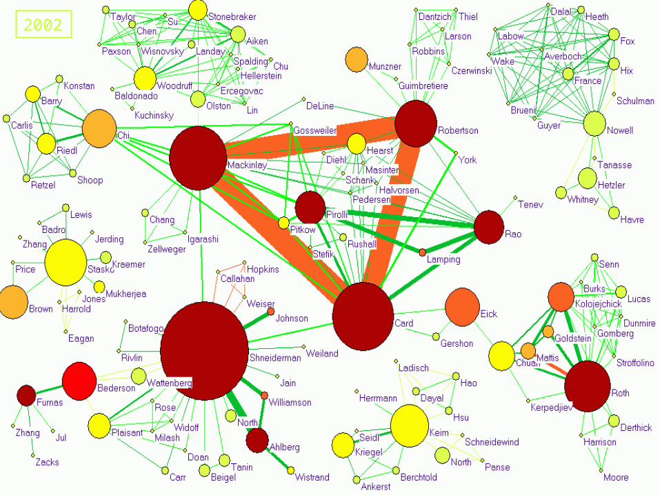
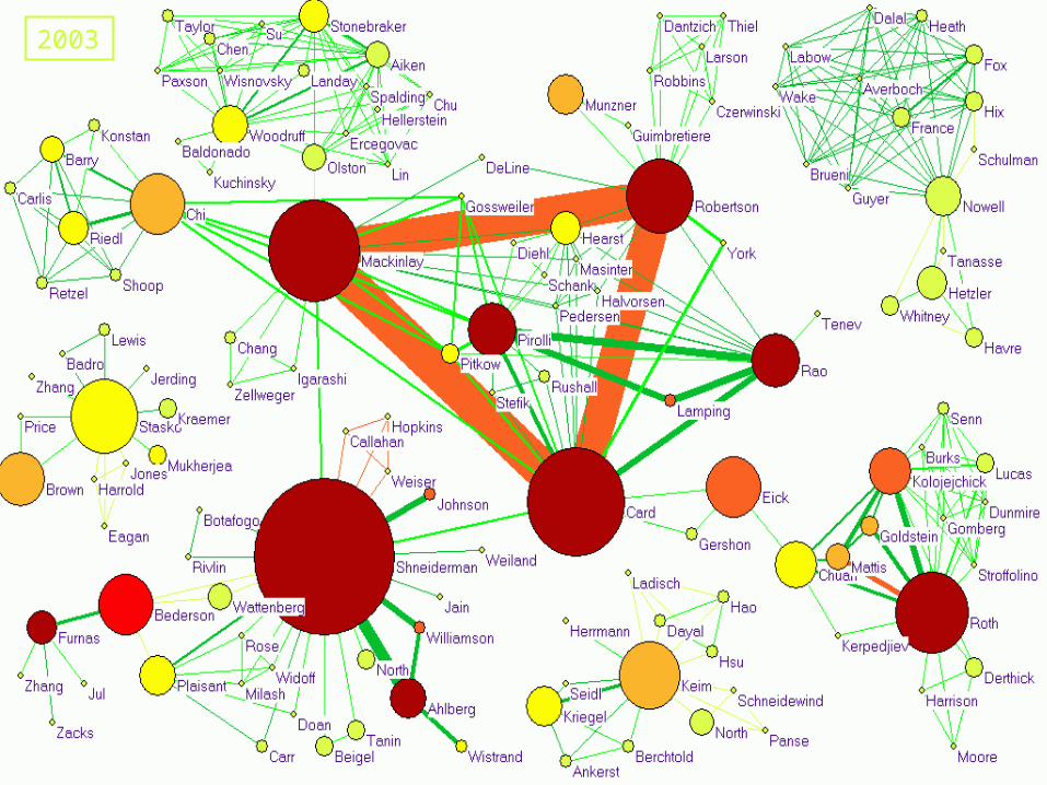
Showing longitudinal data with animations

1988

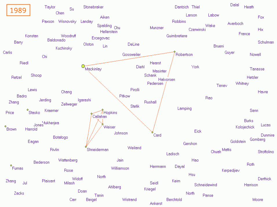
1989

1990

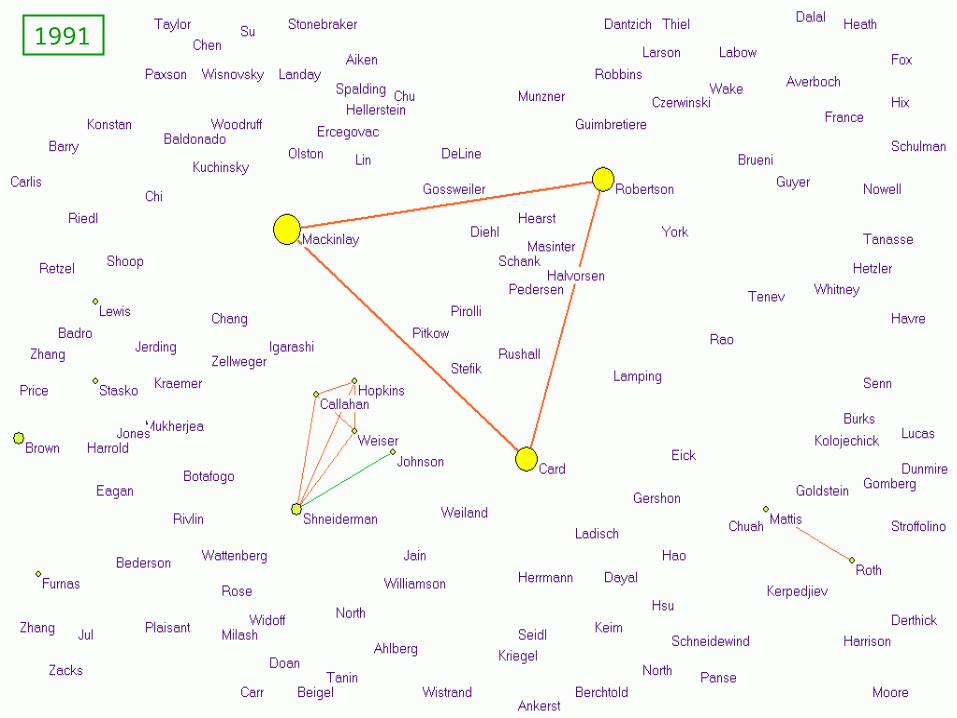
1991

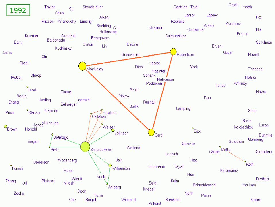
1992

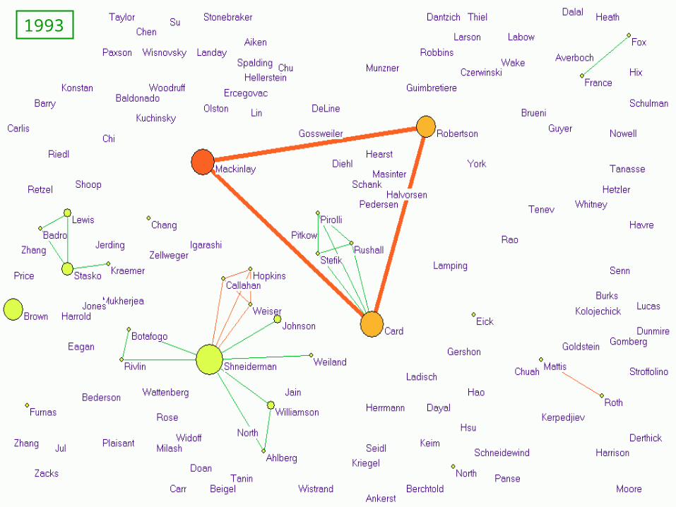
1993

1994

1995

1996

1997

1998

1999

2000

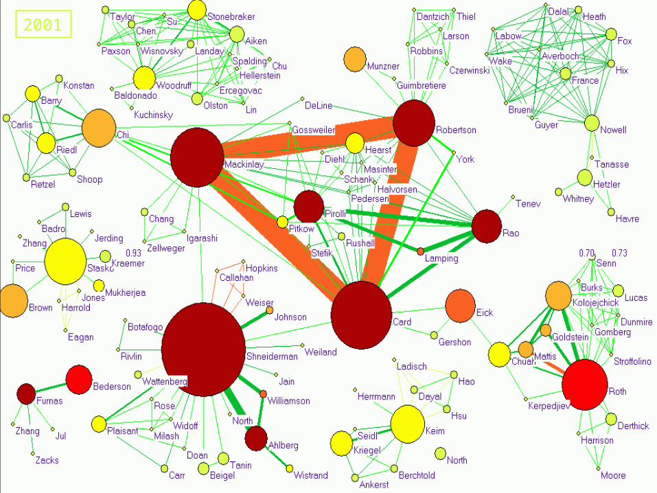
2001

2002

2003

2004

Displaying longitudinal data through animation

Nodes should move little between different timepoints to make it easier to track them

Most people can track 3-7 objects simultaneously (your network can have hundreds or more)

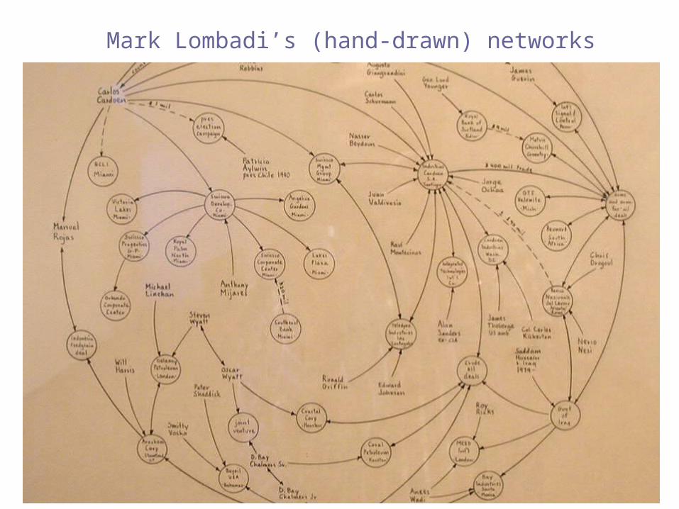
Mark Lombadi’s (hand-drawn) networks

What else could be added to this visualization?

What else could be added to this visualization?

Visualizing attributes (gender)

High school dating: Data drawn from Peter S. Bearman, James Moody, and Katherine Stovel, Chains of affection: The structure of adolescent romantic and sexual networks, American Journal of Sociology 110, 44-91 (2004).

(Image by Mark Newman)

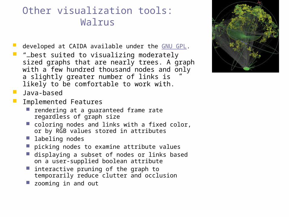
Other visualization tools: Walrus

developed at CAIDA available under the GNU GPL. “…best suited to visualizing moderately sized graphs

that are nearly trees. A graph with a few hundred thousand nodes and only a slightly greater number of links is likely to be comfortable to work with.”

Java-based Implemented Features

rendering at a guaranteed frame rate regardless of graph size

coloring nodes and links with a fixed color, or by RGB values stored in attributes

labeling nodes picking nodes to examine attribute values displaying a subset of nodes or links based on a user-

supplied boolean attribute interactive pruning of the graph to temporarily reduce

clutter and occlusion zooming in and out

Other visualization tools: GraphViz

Takes descriptions of graphs in simple text languages Outputs images in useful formats Options for shapes and colors Standalone or use as a library

dot: hierarchical or layered drawings of directed graphs, by avoiding edge crossings and reducing edge length

neato (Kamada-Kawai) and fdp (Fruchterman-Reinhold with heuristics to handle larger graphs)

twopi – radial layout circo – circular layout

http://www.graphviz.org/

Dot (GraphViz)

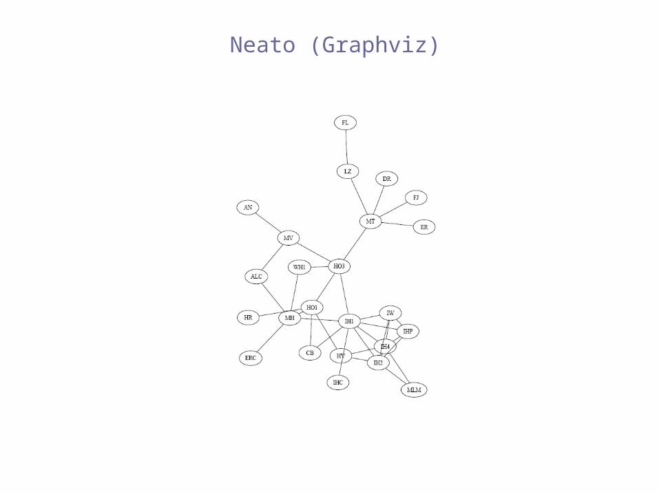
Neato (Graphviz)

Summary

What we covered snowball sampling clustering coefficient network visualization

What we didn’t cover countless other visualization tools 3D, etc.