SCHOOL OF ENGINEERING & BUILT ENVIRONMENT

Mathematics

Basic Algebra

1. Operations and Expressions 2. Common Mistakes 3. Division of Algebraic Expressions 4. Exponential Functions and Logarithms 5. Operations and their Inverses 6. Manipulating Formulae and Solving Equations 7. Quadratic Equations – A Reminder 8. Simultaneous Equations – A Reminder

Tutorial Exercises

Dr Derek Hodson

Contents Page 1. Operations and Expressions ................................................................................ 1 2. Common Mistakes .............................................................................................. 4 3. Division of Algebraic Expressions ...................................................................... 4 4. Exponential Functions and Logarithms .............................................................. 8 5. Operations and their Inverses .............................................................................. 10 6. Manipulating Formulae and Solving Equations ................................................... 11 7. Quadratic Equations – A Reminder ..................................................................... 24 8. Simultaneous Equations – A Reminder ............................................................... 25 Tutorial Exercises ................................................................................................ 27 Answers to Tutorial Exercises ............................................................................. 33

1

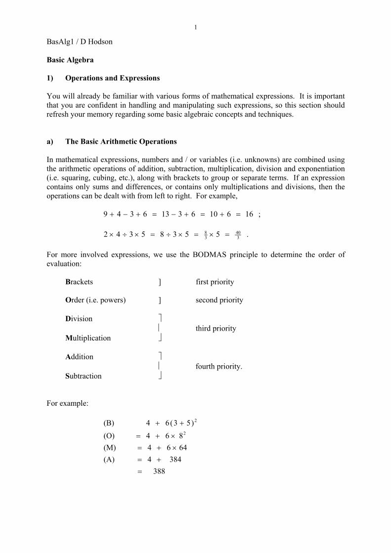
BasAlg1 / D Hodson Basic Algebra 1) Operations and Expressions You will already be familiar with various forms of mathematical expressions. It is important that you are confident in handling and manipulating such expressions, so this section should refresh your memory regarding some basic algebraic concepts and techniques. a) The Basic Arithmetic Operations In mathematical expressions, numbers and / or variables (i.e. unknowns) are combined using the arithmetic operations of addition, subtraction, multiplication, division and exponentiation (i.e. squaring, cubing, etc.), along with brackets to group or separate terms. If an expression contains only sums and differences, or contains only multiplications and divisions, then the operations can be dealt with from left to right. For example, 1661063136349 =+=+−=+−+ ; 3

4038 55385342 =×=×÷=×÷× .

For more involved expressions, we use the BODMAS principle to determine the order of evaluation: Brackets ] first priority Order (i.e. powers) ] second priority Division ⎤ ⎥ third priority Multiplication ⎦ Addition ⎤

⎥ fourth priority. Subtraction ⎦ For example:

3883844(A)

6464(M)864(O)

)53(64(B)2

2

=+=

×+=×+=

++

2

Another example:

268(S)

62

16(D)

62

4(O)

62

)31((B)

2

2

=−=

−=

−=

−+

b) Indices (Powers) The simple use of powers or indices to represent repeated multiplication should be familiar, for example aaa ×=2

aaaa ××=3

, ]terms[... naaaaa n ×××= but you must also be clear on the wider interpretation of indices. The lines below collate the important aspects of indices:

• 1 0 =a

• nn

aa 1

=− and nn a

a=−

1

• aa =21 and m aa m =

1

• mn mn aaa +=

• mnm

n

aaa −=

• nmmn aa =)(

• mmm baba =)(

• m

mm

ba

ba

=⎟⎠⎞

⎜⎝⎛

These results will be needed in both the expansion and simplification of algebraic expressions.

3

Examples (1) (a) Expand . )65()73( 2222 yxyx −+

4224

422224

2222222222

42171542351815

)65(7)65(3)65()73(

yyxxyxyyxxyxyyxxyxyx

−+=

−+−=

−+−=−+

(b) Expand . 3)4( +x

64481264324168

)168(4)168()168()4(

)4()4()4(

23

223

22

2

23

+++=

+++++=

+++++=

+++=

++=+

xxxxxxxxxxxxx

xxxxxx

(c) Simplify 824

32

3)(15

zyxzyx .

23

213

824

63

824

32

5

5

315

3)(15

zxy

zyx

zyxzyx

zyxzyx

=

=

=

−−

See the Tutorial Exercises for practice.

4

2) Common Mistakes Here are just a few common mistakes to avoid when manipulating algebraic expressions:

• 3 : 3 2)2( xx = 3333 82)2( xxx ==

• 22 : 2 2)( yxyx +=+ 22 2)( yyxxyx ++=+

• db

ca

dcba

+=++ :

dcb

dca

dcba

++

+=

++

• caba : ccba =)( bacba =)(

• nm : nm aaa +=+ nmnm aaa =+

• 33 2

21 −= xx

: 33 2

12

1 −= xx

3) Division of Algebraic Expressions Providing the denominator (i.e. the bottom bit) of a division contains no +’s or −’s, the division itself is usually straightforward to carry out. Examples

352

26

210

24

26104

2

2323

+−=

+−=+−

aa

aa

aa

aa

aaaa

(2) (a) (b)

)3(2

62

424

48

424

2

2

23

2

32

2

2332

xyx

xyx

yxyx

yxyx

yxyxyx

−=

−=

−=−8

When the denominator does contain +’s and / or −’s, we may require polynomial division. Note: , , are examples of polynomials.32 +x 542 +− xx 623 23 +−+ xxx

5

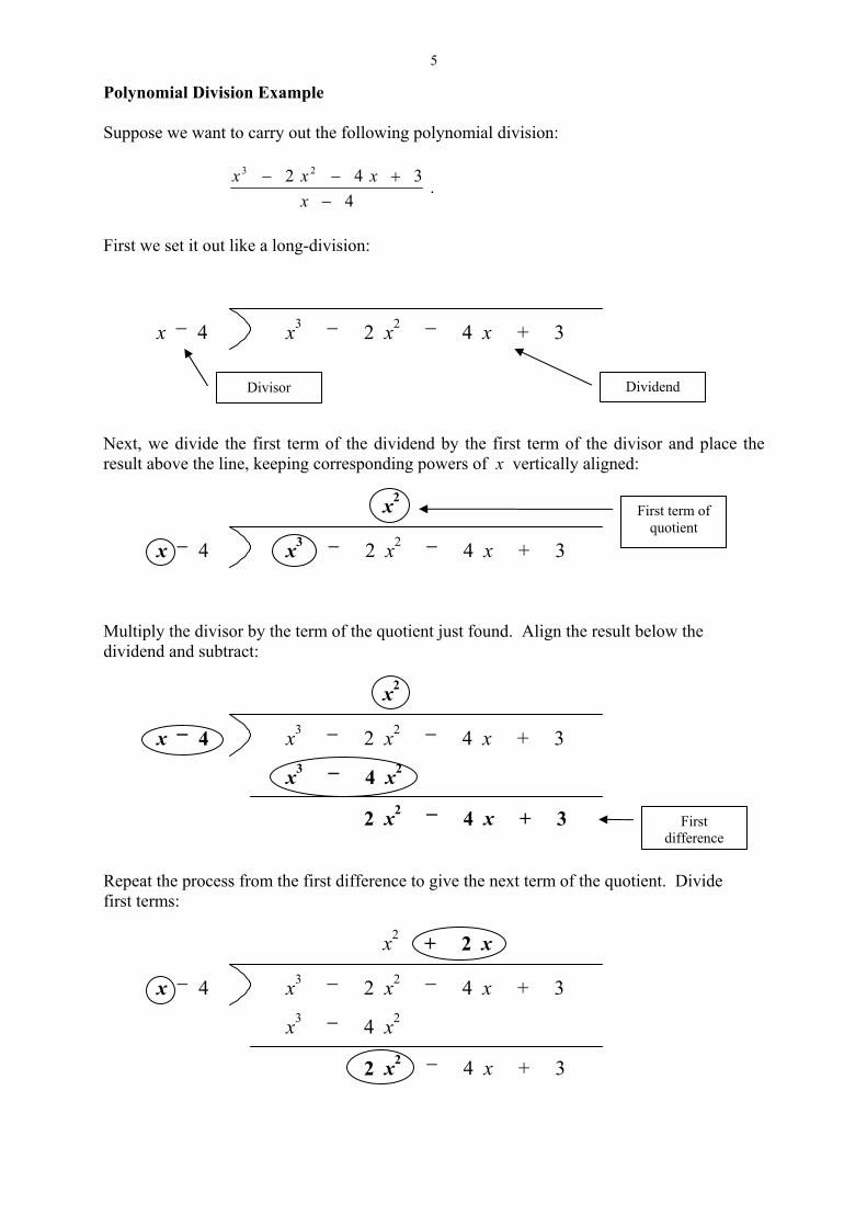
Polynomial Division Example Suppose we want to carry out the following polynomial division:

4

342 23

−+−−

xxxx .

First we set it out like a long-division:

x3 − 2 x2 − 4 x + 3 x − 4

Dividend Divisor

Next, we divide the first term of the dividend by the first term of the divisor and place the result above the line, keeping corresponding powers of x vertically aligned:

x2 + 2 x + 4

x3 − 2 x2 − 4 x + 3 x − 4

First term of quotient

Multiply the divisor by the term of the quotient just found. Align the result below the dividend and subtract:

x2 + 2 x + 4

x3 − 2 x2 − 4 x + 3

x3 − 4 x2 − 4 x + 3

x3 − 2 x2 − 4 x + 3

x − 4

First difference

Repeat the process from the first difference to give the next term of the quotient. Divide first terms:

x2 + 2 x + 4

x3 − 2 x2 − 4 x + 3

x3 − 4 x2 − 4 x + 3

x3 − 2 x2 − 4 x + 3

x − 4

6

Multiply divisor and subtract:

x2 + 2 x + 4

x3 − 2 x2 − 4 x + 3

x3 − 4 x2 − 4 x + 3

x3 − 2 x2 − 4 x + 3

x3 − 2 x2 − 8 x + 3

x3 − 2 x2 − 4 x + 3

x − 4

Second difference

Repeat to complete quotient and determine the remainder:

x2 + 2 x + 4

x3 − 2 x2 − 4 x + 3

x3 − 4 x2 − 4 x + 3

x3 − 2 x2 − 4 x + 3

x3 − 2 x2 − 8 x + 3

x3 − 2 x2 − 4 x + 3

x − 4

x2 + 2 x + 4

x3 − 2 x2 − 4 x + 3

x3 − 4 x2 − 4 x + 3

x3 − 2 x2 − 4 x + 3

x3 − 2 x2 − 8 x + 3

x3 − 2 x2 − 4 x + 3

x3 − 2 x2 − 4 x − 16

x3 − 2 x2 − 4 x + 19

x − 4

Remainder

7

Removing the annotation we have

x2 + 2 x + 4

x3 − 2 x2 − 4 x + 3

x3 − 4 x2 − 4 x + 3

x3 − 2 x2 − 4 x + 3

x3 − 2 x2 − 8 x + 3

x3 − 2 x2 − 4 x + 3

x3 − 2 x2 − 4 x − 16

x3 − 2 x2 − 4 x + 19

x − 4

. In general,

Divisor

RemainderQuotientDivisor

Dividend+= ,

so for the above example we can write

4

19424

342 223

−+++=

−+−−

xxx

xxxx .

Important note: Care must be taken when any of the polynomials have “missing terms”. These should be included with zero coefficients to ensure correct alignment and to minimise mistakes. For example, if we have , 1

1

2 23 −+ xx then this should be written as . 02 23 −++ xxx

8

4) Exponential Functions and Logarithms An exponent is another name for a power or index. Exponents can be used to create exponential functions: . )1,0:0(, ≠>= aaay x

In this context, a is called the base of the exponential function. Commonly used bases are 10 and the exponential constant : 71828.2≈e ; xy 10= . xey = The function with the exponential constant e as its base is so important in mathematics, science and engineering that it is referred to as the exponential function, all others being subordinate. Related to exponential functions are logarithms. If we express a number N as a power of a, i.e. , xaN = then the power is defined to be the (base a ) logarithm of N : ( log of N to the base a ) Nx alog= Note that because of the importance of the exponential constant, logarithms to base e are given the special name of natural logarithms and denoted by . )(ln Examples (3) (a) → 210100 = 2)100(log10 = (b) → 3101000 = 3)1000(log10 = (c) → 6264 = 6)64(log2 = The definition can be extended to fractional powers with logarithms to base 10 and base e obtainable from calculators: (4) (a) (to 6 decimal places) 698970.2)500(log10 = (b) (to 7 decimal places) 7376696.3)42(ln =

9

Because logs are by definition indices, we can use the rules for combining indices to determine the so-called laws of logarithms:

• S [L1] RSR aaa loglog)(log +=

• SRSR

aaa logloglog −=⎟⎠⎞

⎜⎝⎛ [L2]

• Rn . [L3] R an

a log)(log =

We can use these to expand or contract expressions involving logarithms: Examples

(5) (a) Expand ⎟⎟⎠

⎞⎜⎜⎝

⎛2

43

10logz

yx .

]L3[)(log2)(log4)(log3

]L1[)(log)(log)(log

]L2[)(log)(loglog

101010

210

410

310

210

43102

43

10

zyx

zyx

zyxz

yx

−+=

−+=

−=⎟⎟⎠

⎞⎜⎜⎝

⎛

(b) Write )(ln3)(ln6)(ln4 yzyx −++ as a single logarithm.

]L2[)(ln

]L1[)(ln])([ln

]L3[)(ln])([ln)(ln)(ln3)(ln6)(ln4

3

64

364

364

⎥⎦

⎤⎢⎣

⎡ +=

−+=

−++=−++

yzyx

yzyx

yzyxyzyx

We shall return to exponentials and logs later.

10

5) Operations and their Inverses Each basic arithmetic operation that we may encounter (with a few exceptions) has associated with it a corresponding inverse operation. An operation and its inverse, when applied in sequence, effectively cancel out one and other. For example, suppose we start off with x . If we now add a and then subtract a , we are back to x again. That is, xaax =−+ . We can say that the inverse of adding a is subtracting a (and also vice versa!). Similarly, if we multiply x by a , then divide by a , we are again back to x :

xaxa

= .

So the inverse of multiplying by a is dividing by a (and vice versa). The table below shows operations and their inverses, including the exponentials and logs from the previous section, and some others you may already be familiar with:

xaax =−+ xaax =+−

xaxa

= xaax

=

xxba

ab =

This is a special case of the entry above. Multiplying by ba is

the same as multiplying by a and dividing by b. Hence the

inverse operation is multiplying by ab .

xx =2 or xx =21)( 2 ( ) xx =

2 or xx =2)( 2

1

xx =3 3 or xx =31)( 3 ( ) xx =

33 or xx =3)( 3

1

xxn n = or xx nn =1)( ( ) xx

nn = or xx nn =)( 1

xx =10log10 xx =)10(log10

xe x =ln xe x =)(ln

xx =− )sin(sin 1 xx =− )sin(sin 1

xx =− )cos(cos 1 xx =− )cos(cos 1

xx =− )tan(tan 1 xx =− )tan(tan 1

11

6) Manipulating Formulae and Solving Equations The operation / inverse operation effect described in the previous section provides the key to manipulating formulae and solving equations. A formula is an equation that expresses a relationship between “quantities”. In particular, it expresses how to determine the value of one quantity from the values of one or more other quantities. Below are some examples of formulae that you may have seen before:

• )32(95 −= FC

• 334 rV π=

• 221 tatud +=

• t auv +=

• R iv =

In each of these formulae, the quantity on the left is called the subject of the formula. Often, when working with a formula, we want to change the subject to one of the other quantities. For example:

→ Riv =Rvi = - i is now the subject.

This is a very simple example. However, the manipulation of formulae is an aspect of algebra that can pose difficulties for students. Consider the formula in the above list that relates temperature in degrees Celsius to temperature in degrees Fahrenheit: )32(9

5 −= FC . It is quite easy to make F the subject of this formula. How you would tackle this would probably depend on methods brought from school. If you are thinking something like, “move terms from one side of the equation to the other to get F on its own”, then please think again. Although the “method” of “moving” terms will probably get you the correct answer in this case, it is not a mathematically correct way of thinking and can cause problems in more complicated formulae. Let us now look at the correct way to manipulate a formula or equation. This will let you see what is really happening when terms appear to “move” around an equation. Warning: Ignore the following at your peril!

12

First, let us look at the formula as given and the mathematical operations within it: )32(9

5 −= FC . Given a value of F , (following BODMAS) we would determine the corresponding value of C by:

• subtracting 32

• multiplying by 95 .

A formula (or, in fact, any equation) is like a balanced set of scales:

C )32(95 −F =

When working with an equation, we must not upset the balance. This means that if we do something to one side of the equation, then we must do the exact same thing to the other side. This is the one and only rule of algebraic manipulation. [Note: We can, of course, swap the sides around, but that is just like turning the scales around; it does not affect the balance.] To change the subject of a formula, we apply carefully chosen operations to both sides of the equation whose net effect is to isolate the new subject. These operations are the inverse operations of the those within the original formula. That is:

• subtract 32

• multiply by 95

are reversed and inverted to give

• multiply by 59

• add 32 .

These operations are now applied, in turn, to both sides of the equation.

13

The process in full is as follows: )32(9

5 −= FC Multiply both sides by 5

9 : )32(95

59

59 −= FC

)32(5

9 −= FC 325

9 −= FC Add 32 to both sides: 3232325

9 +−=+ FC FC =+ 325

9 Swap sides: 325

9 += CF ... and with pictures:

C )32(95 −F =

Formula:

C59 )32(9

559 −F =

Multiply both sides by 59 :

C59 32−F =

3259 +C 3232 +−F=

Add 32 to both sides:

3259 +C F =

F 3259 +C =

Swap sides:

14

In practice, we needn’t put in as much detail. For such a simple formula we might simply set down the following lines: )32(9

5 −= FC Multiply both sides by 5

9 : 3259 −= FC

Add 32 to both sides: FC =+ 325

9 Swap sides: 325

9 += CF . This abbreviated version may give the impression that terms are moving around the equation, but they are not. You must always keep in mind what is truly happening in the background. Always think BALANCE. Further Examples Note: In the following examples, full details are shown. In practice, the level of detail you

show in you own working will depend on your own confidence and ability; as these grow, you will naturally display less.

(6) For the formula make x the subject. 243 xy += [Note: This is the same as saying, solve for x .] Analyse operations. Given x, how is y calculated?

• square • multiply by 4 • add 3

Reverse and invert operations:

• subtract 3 • divide by 4 • square root

15

Apply inverse operations to formula: Formula: 243 xy += Subtract 3 : 3433 2 −+=− xy 243 xy =−

Divide by 4 : 4

44

3 2xy=

−

2

43 xy

=−

At this point it is useful to swap sides

4

32 −=

yx

Square root: 4

32 −=

yx

4

3−=

yx

Shortened version (for the more confident): Formula: 243 xy += Subtract 3 : 243 xy =−

Swap sides and divide by 4 : 4

32 −=

yx

Square root: 4

3−=

yx

16

(7) For the formula 334 rV π= , make r the subject.

Analyse operations. Given r , how is V calculated?

• cube (or raise to the power 3) • multiply by 3

4π Reverse and invert operations:

• multiply by π43

• cube root (or raise to the power 31 )

Apply inverse operations to formula: Formula: 3

34 rV π=

3

34 rV π=

Multiply by π4

3 : 33

443

43 rV π

ππ = 3

43 rV =π

Swap sides: π4

33 Vr = Raise to the power 3

1 : ( ) ( ) 31

31

433πVr =

( ) 3

1

43πVr =

Shortened version: Formula: 3

34 rV π=

Swap sides and multiply by π4

3 : π433 Vr =

Raise to the power 3

1 : ( ) 31

4πr = 3V

17

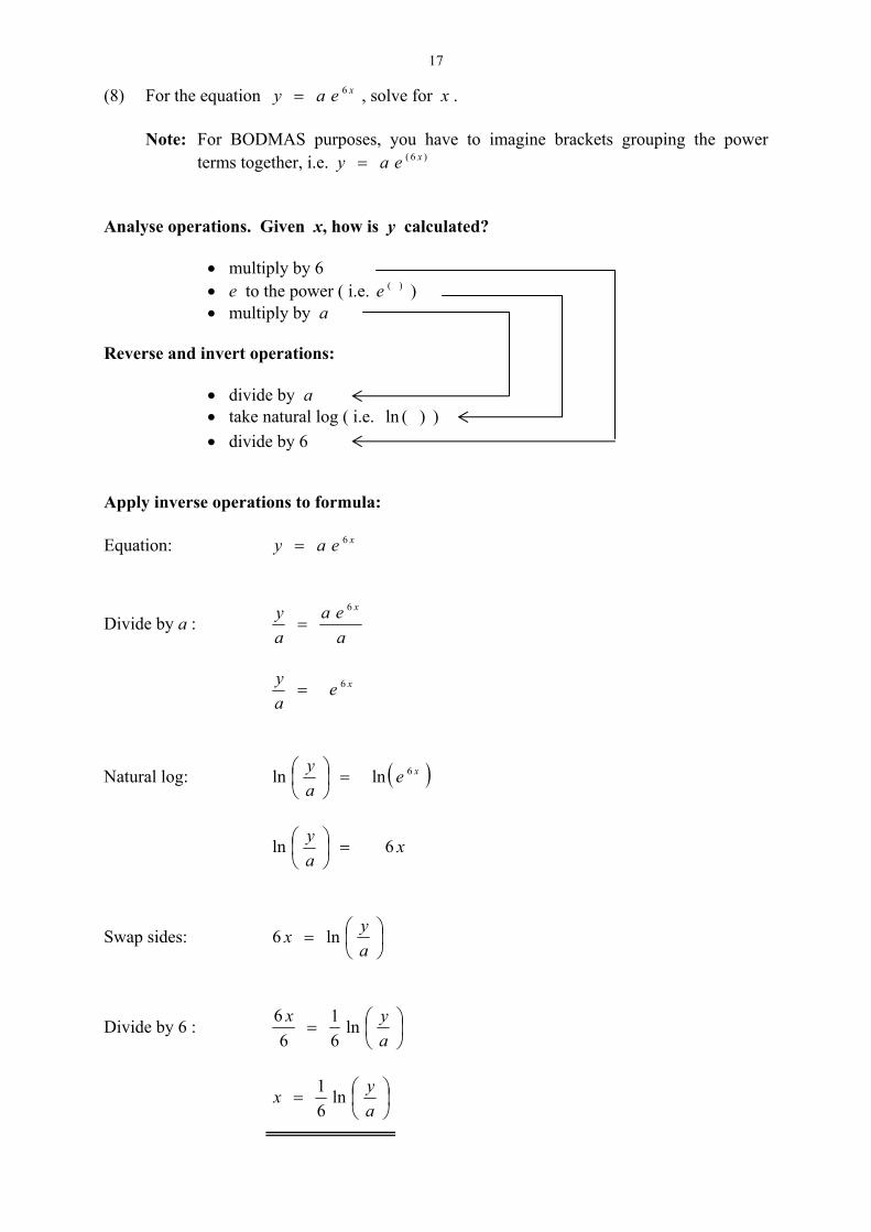
(8) For the equation , solve for x . xeay 6= Note: For BODMAS purposes, you have to imagine brackets grouping the power

terms together, i.e. )6( xeay = Analyse operations. Given x, how is y calculated?

• multiply by 6 • e to the power ( i.e. )(e ) • multiply by a

Reverse and invert operations:

• divide by a • take natural log ( i.e. )(ln ) • divide by 6

Apply inverse operations to formula: Equation: xeay 6=

Divide by a : aea

ay x6

=

xeay 6=

Natural log: ( )xeay 6lnln =⎟⎠⎞

⎜⎝⎛

xay 6ln =⎟⎠⎞

⎜⎝⎛

Swap sides: ⎟⎠⎞

⎜⎝⎛=

ayx ln6

Divide by 6 : ⎟⎠⎞

⎜⎝⎛=

ayx ln

61

66

⎟⎠⎞

⎜⎝⎛=

ayx ln1

6

18

Shortened version: Equation: xeay 6=

Divide by a : xeay 6=

Swap sides and take natural log: ⎟⎠⎞

⎜⎝⎛=

ayx ln6

Divide by 6 : ⎟⎠⎞

⎜⎝⎛=

ayx ln

61

Examples (with less detail): (9) Determine t when . 810 5.0 =t

This is not a formula with a subject, so we cannot write down a sequence of operations. It is, however, an equation (with an unknown) and the concept of balance still applies. In manipulating this equation, we want to end up with the form )(=t . Clearly we must manipulate t down to the level of the equals sign. One of the laws of logarithms will help here: Equation: 810 5.0 =t

Take log (base 10) of both sides: ( ) )8(log10log 10

5.010 =t

)8(log5.0 10=t

Multiply both sides by 2 : )8(log25.02 10=× t

)8(log2 10=t 8062.1≈t

19

(10) Determine t when . 5.04 =− te Equation: 5.04 =− te Take natural log of both sides: ( ) )5.0(lnln 4 =− te

)5.0(ln4 =− t Divide both sides by : 4− )5.0(ln4

1−=t (same as multiplying by 4

1− ) 1733.0≈t (11) Determine x when . 62 4 =x

Equation: 62 4 =x

Take log (base 10) of both sides: ( ) )6(log2log 10

410 =x

)6(log)2(log4 1010 =x

Divide both sides by : )2(log4 10 )2(log4)6(log

10

10=x

6462.0≈x Note: You could use natural logs and get the same answer.

20

Applied Examples (12) The current (i) in the branch of an electronic circuit changes with time (t) in line with

the formula . tkeii −= 0

The initial current (i.e. when 0=t ) is 15 mA. It takes for the current to drop to

(i.e. half its initial value). s7.4

mA5.7 (i) From the numerical information given, determine the values of the parameters

and k . 0i

(ii) Determine the current when s5.6=t . (iii) Determine t when the current is 25% of its initial value. (i) When , 0=t 15=i (Note: As long as we are consistent, we don’t need to convert mA

to A). Input these values into the formula: 0.

015 kei −= 1

5

.15 0i= → 10 =i tkei −= 15 When , 7.4=t 5.7=i . Input these values into the updated formula and solve for k : ke 7.4155.7 −= 5.07.4 =− ke ( ) )5.0(lnln 7.4 =− ke )5.0(ln7.4 =− k

147478123.07.4

)5.0(ln≈

−=k

Completed formula is: i ; we use this to answer the remaining parts. te 14748.015 −=

21

(ii) Set in formula and evaluate i : 5.6=t . m75.515 5.614748.0 == ×−ei A

5

(iii) ; set in formula and solve for t : 75.315of%25 = 75.3=i te 14748.01575.3 −= 2.014748.0 =− te ( ) )25.0(lnln 14748.0 =− te

)25.0(ln14748.0 =− t

s40.914748.0

)25.0(ln=

−=t .

(13) The decay of the radioactive element radium is modelled by the formula

16200 )5.0(

tAA =

where is the initial amount of radium and A is the amount remaining after t years. 0A (i) How much radium remains in a 1 kg sample after 1000 years? (ii) How long would it take for a 1 kg sample to decay to 0.01 kg? (i) Set , in formula and evaluate: 10 =A 1000=t

kg6519.0)5.0( 16201000

==A . (ii) Set , 10 =A 01.0=A in formula and solve for t :

1620)5.0(01.0t

=

)01.0(ln)5.0(ln 1620 =t

)01.0(ln)5.0(ln1620

=t

years10763)5.0(ln

)01.0(ln1620==t

22

(14) In the formula

21

21

RRRR

R+

=

make the subject. 1R Because the new subject appears in more than one position in the formula, we cannot deconstruct the formula into a sequence of operations that reveal how it should be manipulated. This means we have to try and determine the appropriate operations as we go. Ultimately, we want to achieve to form , only)and with expression( 21 RRR = so we must manipulate the equation in such a way that the are combined. Fractions can be awkward to handle, so let us get rid of the fraction.

s'1R

Multiply both sides of the formula by the denominator 21 RR + :

21

212121 )()(

RRRRRRRRR+

+=+

This simplifies to 2121 )( RRRRR =+ . Now multiply out the brackets: 2121 RRRRRR =+ . Subtract from both sides: RR1

RRRRRRRRRR 121121 −=−+ RRRRRR 1212 −= .

1R now appears on one side of the equation and at the same level. Swap sides and take out a common factor: RRRRR 221 )( =− . Now divide both sides by to give the desired result: RR −2

RR2

RRR−

= 21 .

See over for the shortened version with less detail:

23

Formula: 21

21

RRRRR+

=

Manipulations: 2121 )( RRRRR =+ . 2121 RRRRRR =+ . RRRRRR 1212 −= . RRRRR 221 )( =− .

RR

RRR−

=2

21 .

The above examples illustrate the process of algebraic manipulation, but every possible twist and turn cannot be covered. You must now develop your understanding of the process through practice and be prepared to wrestle with problems to achieve a result.

24

7) Quadratic Equations – A Reminder One type of equation that crops up quite frequently is the quadratic equation: . 02 =++ cxbxa This type of equation is solved either by factorisation (which isn’t always possible) or by use of the quadratic formula

a

cabbx

242 −±−

= .

Examples (15) (a) Solve by factorisation. 0822 =−+ xx 0

0

822 =−+ xx )2()4( =−+ xx

→ ⎪⎭

⎪⎬

⎫

=−

=+

0)2(or

0)4(

x

x

⎪⎭

⎪⎬

⎫

+=

−=

2or

4

x

x

(b) Solve +x by the quadratic formula. 0822 =−x → 0822 =−+ xx 8,2,1 −=== cba

2or4

24or

28

262

2362

12)8(1422

24

2

2

−=

−=

±−=

±−=

×−××−±−

=

−±−=

acabb

x

Note: Quadratic equations may have two real solutions, one real solution or no real

solutions, depending on the value of the discriminant cab 42 − .

25

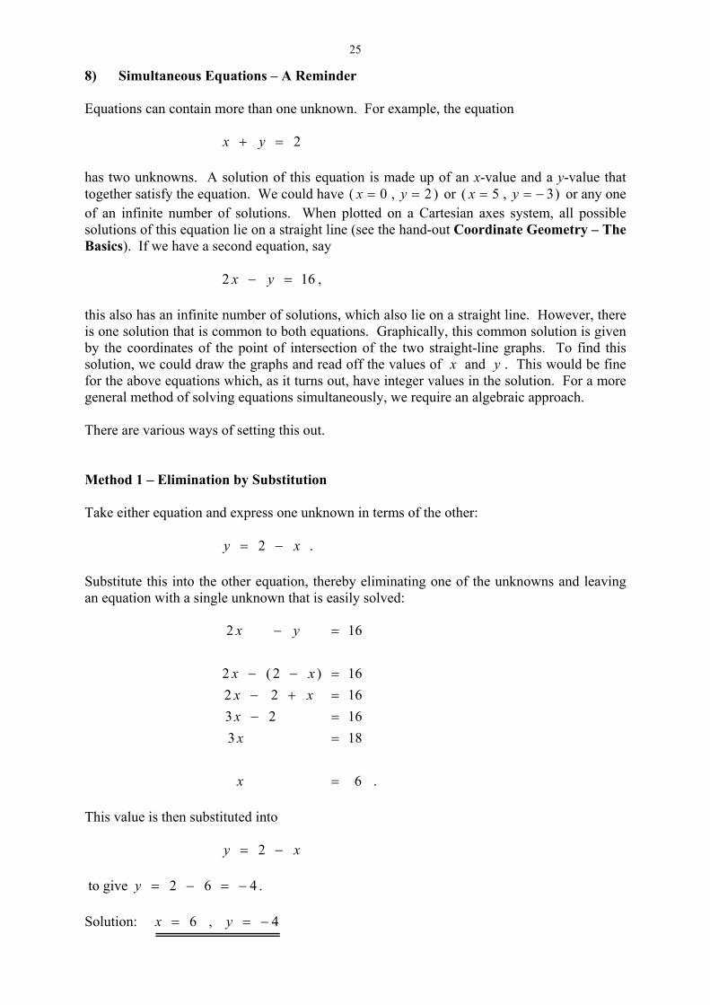
8) Simultaneous Equations – A Reminder Equations can contain more than one unknown. For example, the equation 2=+ yx has two unknowns. A solution of this equation is made up of an x-value and a y-value that together satisfy the equation. We could have )2,0( == yx or )3,5( −== yx or any one of an infinite number of solutions. When plotted on a Cartesian axes system, all possible solutions of this equation lie on a straight line (see the hand-out Coordinate Geometry – The Basics). If we have a second equation, say , 12 =− yx 6 this also has an infinite number of solutions, which also lie on a straight line. However, there is one solution that is common to both equations. Graphically, this common solution is given by the coordinates of the point of intersection of the two straight-line graphs. To find this solution, we could draw the graphs and read off the values of x and y . This would be fine for the above equations which, as it turns out, have integer values in the solution. For a more general method of solving equations simultaneously, we require an algebraic approach. There are various ways of setting this out. Method 1 – Elimination by Substitution Take either equation and express one unknown in terms of the other: . xy −= 2 Substitute this into the other equation, thereby eliminating one of the unknowns and leaving an equation with a single unknown that is easily solved:

.6

1831623162216)2(2

162

=

==−=+−=−−

=−

x

xx

xxxx

yx

This value is then substituted into xy −= 2 to give . 462 −=−=y Solution: 4−== y,6x

26

Method 2 – Elimination by the Addition or Subtraction of Equations Line up the equations one above the other:

.162

2=−=+

yxyx

If necessary, multiply up one or other or both equations to obtain common coefficients on one of the unknowns:

or 1622

=−=+

yxyx

.162422

=−=+

yxyx

Next, eliminate the unknown with the common coefficient by adding or subtracting corresponding sides of the equations:

6:Solve183:Add

1622

==

=−=+

xx

yxyx

or

.4:Solve123:Subtract

162422

−=−=

=−=+

yy

yxyx

Solution: 4,6 −== yx Whichever method you use, always check your answers by substituting the values into the original equations:

RHS2

)4(6LHS :equation1st

==

−+=+= yx

. RHS16

412)4(62

2LHS :equation 2nd

==

+=−−×=

−= yx

27

Tutorial Exercises (1) Expansion of Algebraic Expressions Containing Brackets (Revision) (1.1) Expand the following expressions involving products and powers: (i) (ii) )9 )5()3( 42 xx ()8( 53 xx (iii) (iv) )7()4( 32 yxyx )6()3( 9843 yxyx− (v) (vi) )7()5( 9372 yxyx − )5()3( 2 baba − (vii) (viii) )8()5( 232 yxyx −− )4()3( 32 baba −− (ix) (x) . )()()4( 2 babaa − 222 )()4()3( bababa −− (1.2) Open out the following bracketed expressions: (i) )3()2( ++ xx (ii) )73()52( −+ xx (iii) (iv) )32()32( +− xx )136()84( −− yy (v) (vi) 2)4( +x 2)32( yx + (vii) (viii) 2)32( yx − )54()2( 2 +−+ xxx (ix) (x) )73()12( 2 +−− xxx )5()4()3( +−+ xxx . (1.3) Factorise the following quadratic expressions: (i) (ii) 232 ++ xx 452 ++ xx (iii) (iv) 2 442 ++ xx 2 −+ xx (v) (vi) 6 22 −− xx 52 −+ xx (vii) (viii) 6 652 −− xx 2 −+ xx (ix) (x) . 62 −− xx 12112 2 ++ xx (1.4) Show that and use the result to 22)()( bababa −=−+ (i) expand: ; )2()2( −+ xx )32()32( +− xx (ii) factorise: ; . 162 −x 6425 2 −x

28

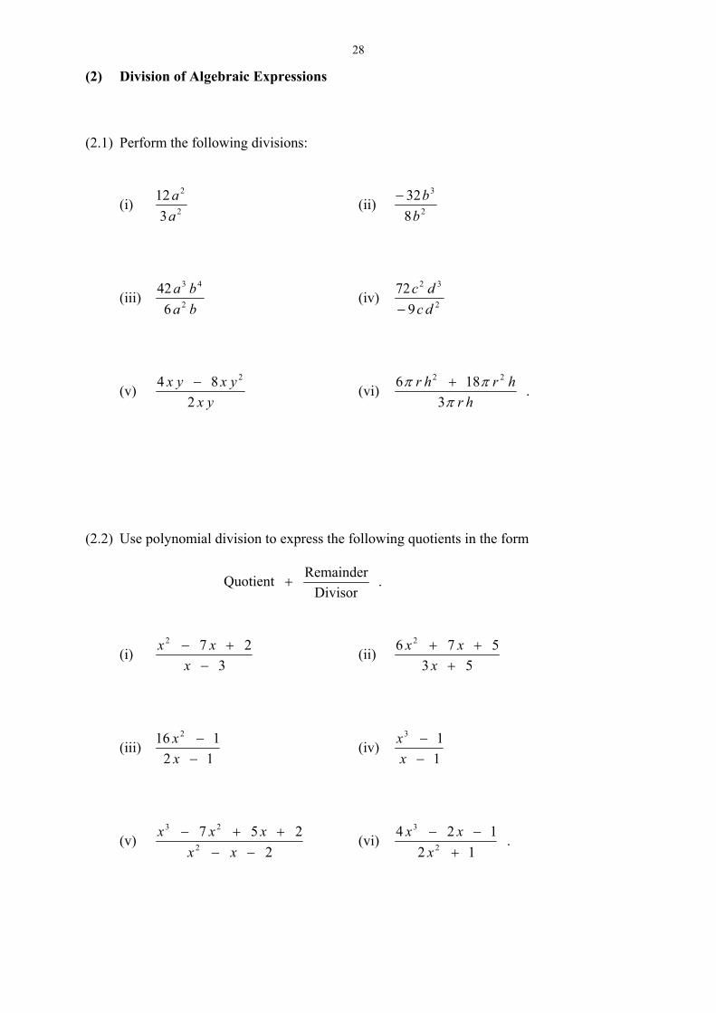
(2) Division of Algebraic Expressions (2.1) Perform the following divisions:

(i) 2

2

312

aa (ii) 2

3

832b

b−

(iii) baba

2

43

642 (iv) 2

32

972

dcdc

−

(v) yx

yxyx2

84 2− (vi) hr

hrhrπ

ππ3

186 22 + .

(2.2) Use polynomial division to express the following quotients in the form

Divisor

RemainderQuotient + .

(i) 3

272

−+−

xxx (ii)

53576 2

+++

xxx

(iii) 12116 2

−−

xx (iv)

113

−−

xx

(v) 2

2572

23

−−++−

xxxxx (vi)

12124

2

3

+−−

xxx .

29

(3) Exponentials and Logarithms – The Basics (3.1) Use your calculator functions, namely log (which is actually ) and , to

evaluate the following expressions. Comment on the results for parts (v) – (viii). 10log x10

(i) (ii) )1000(log10 )5.2(log10

(iii) (iv) 5.310 4.110 −

(v) (vi) ) )10(log 5.3

10 10(log 4.110

−

(vii) (viii) . )1.6(log1010 )5.0(log1010 (3.2) Use your calculator functions, namely ln (which is actually ) and , to evaluate

the following expressions. Comment on the results for parts (v) – (viii). elog xe

(i) (ii) )5.4(ln )75.2(ln (iii) (iv) 6.0e 5.1−e (v) (vi) )(ln 6.0e )(ln 5.1−e (vii) (viii) . )5.2(lne )75.0(lne (3.3) Write each of the following expressions as sums and differences of logarithms (where

possible, without using powers):

(i) ⎟⎟⎠

⎞⎜⎜⎝

⎛yx 2

103log (ii) ⎟⎟

⎠

⎞⎜⎜⎝

⎛4

ln22 yx

(iii) ⎟⎟⎠

⎞⎜⎜⎝

⎛+ 1

100log10 x (iv) ⎟⎟

⎠

⎞⎜⎜⎝

⎛+ 32

ln2

xe

(v) 1log 210 +x (vi)

)2()1()1(ln

3

+−+

xxx .

(3.4) Write each of the following as a single logarithm: (i) zyx 101010 log4log2log3 −+ (ii) zyx 102

110 log)(log2 −+

(iii) yx lnln3 3

1+ (iv) . zyx ln2)2(ln4 −+

30

(4) Changing the Subject of a Formula (4.1) For each of the following formulae, change the subject to the quantity indicated in

brackets: (i) tauv += )( t (ii) 2

21 tas = )( t

(iii) 2

21 tatus += )( u

(iv) 2

21 tatus += )( a

(v) sauv 22 += )( s (vi) sauv 22 += )( u (vii) 3xbay += )( x (viii) tei 5= )( t (ix) tei 28 −= )( t (x) )12(10 += xy )( x (xi) )23(10 −= xy )( x (xii) . tkeacy −+= 00 )( t (4.2) For each of the following formulae, change the subject to the quantity indicated in

brackets:

(i) xxy

+−

=32 (ii) )( x

xxy

−+

=5

24 )( x

(iii) yx

yxz+

= ) (iv) ( y21

21

CCCCC−

= . )( 2C

31

(5) Solution of Equations (5.1) Solve the following equations: (i) (ii) 854 =+x 12810 −=−x (iii) (iv) 5236 −=+ xx 2593 +=− xx (v) (vi) 3235 2 =+ x 03205 3 =+x (vii) (viii) 75.0=xe 2.04 =xe (ix) (x) 785 =−− xe 13124 3 =+ − xe (xi) 2)3(ln −=x (xii) 03)2(ln5 =+x (xiii) (xiv) 10)4(ln35 −=− x 25.0)46(ln =+x (xv) (xvi) 5.210 =x 75.110 23 =−x

(xvii) (xviii) 32.0)4(log10 =x 65.0)45(log10 =+x (xix) (xx) 52 14 =−x 63 42 =+x

(5.2) Solve the following quadratic equations by factorisation, then repeat using the quadratic

formula: (i) (ii) 01522 =−+ xx 02092 =+− xx (iii) (iv) . 025102 =++ xx 0472 2 =−− xx

32

(5.3) The following quadratic equations do not have any real solutions. Try solving them by the quadratic formula and see what happens:

(i) (ii) . 0222 =++ xx 0432 2 =+− xx (5.4) Solve the following sets of simultaneous equations:

(i) (ii) ⎭⎬⎫

=−=+

162234

yxyx

⎭⎬⎫

−=+=+

234125

yxyx

(iii) (iv) . ⎭⎬⎫

−=+−=−

7542026

yxyx

⎭⎬⎫

=−=−

5.10325.2458

yxyx

33

Answers (1.1) (i) (ii) 615 x 872 x (iii) (iv) 4328 yx 131118 yx− (v) (vi) 16535 yx− 3345 ba− (vii) (viii) 3540 yx 4312 ba (ix) (x) 244 ba− 6512 ba (1.2) (i) (ii) 652 ++ xx 356 2 −+ xx (iii) (iv) 10410024 94 2 −x 2 +− yy (v) (vi) 1682 ++ xx 22 9124 yyxx ++ (vii) (viii) 22 9124 yyxx +− 1032 23 +−− xxx (ix) (x) 71772 23 −+− xxx 60174 23 −−+ xxx (1.3) (i) (ii) )2()1( ++ xx )1()4( ++ xx (iii) (iv) 2)2( +x )1()2( −+ xx (v) (vi) )1()2( +− xx )1()6( −+ xx (vii) (viii) )2()1()6( +− xx )3( −+ xx (ix) (x) )2()3( +− xx )4()32( ++ xx (1.4) (i) ; 4)2()2( 2 −=−+ xxx 94)32()32( 2 −=+− xxx (ii) ; )4()4(162 −+=− xxx )85()85(6425 2 −+=− xxx (2.1) (i) (ii) 4 b4− (iii) (iv) 37 ba dc8− (v) (vi) y42 − rh 62 +

34

(2.2) (i) 3

10)4(−

−−x

x (ii) 53

10)12(+

+−x

x

(iii) 12

3)48(−

++x

x (iv) [no remainder] 12 ++ xx

(v) 2

10)6( 2 −−−

+−xx

xx (vi) 12

142 2 ++

−xxx

(3.1) (i) 3 (ii) 0.397940008 (iii) 3162.27766 (iv) 0.039810717 (v) 3.5 (vi) −1.4 (vii) 6.1 (viii) 0.5 (3.2) (i) 1.504077397 (ii) 1.011600912 (iii) 1.822118800 (iv) 0.223130160 (v) 0.6 (vi) −1.5 (vii) 2.5 (viii) 0.75 (3.3) (i) yx 101010 loglog23log −+ (ii) 4lnln2ln2 −+ yx (iii) (iv) )1(log2 10 +− x )32(ln2 +− x (v) )1(log 2

1021 +x

(vi) ])2(ln)1(ln)1(ln3[2

1 +−−++ xxx

(3.4) (i) ⎟⎟⎠

⎞⎜⎜⎝

⎛4

23

10logz

yx (ii) ⎥⎥⎦

⎤

⎢⎢⎣

⎡ +zyx 2

10)(log

(iii) ⎟⎠⎞⎜

⎝⎛ 3

13ln yx (iv) ⎥⎦

⎤⎢⎣

⎡ +2

4)2(lnz

yx

35

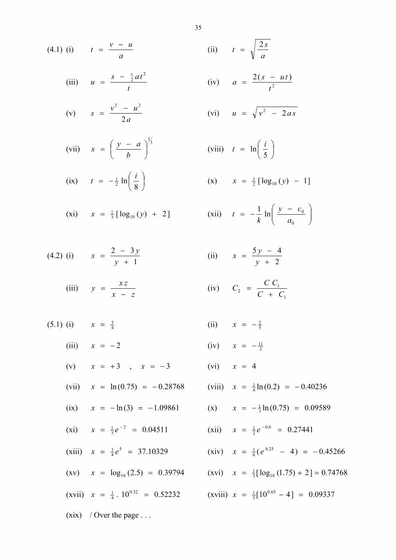
(4.1) (i) a

uvt −= (ii)

ast 2

=

(iii) t

tasu

221−

= (iv) 2

)(2t

tusa −=

(v) a

uvs2

22 −= (vi) savu 22 −=

(vii) 3

1

⎟⎠⎞

⎜⎝⎛ −

=b

ayx (viii) ⎟⎠⎞

⎜⎝⎛=

5ln it

(ix) ⎟⎠⎞

⎜⎝⎛−=

8ln2

1 it (x) ]1)(log[ 1021 −= yx

(xi) ]2)(log[ 1031 += yx (xii) ⎟⎟

⎠

⎞⎜⎜⎝

⎛ −−=

0

0ln1a

cyk

t

(4.2) (i) 1

32+−

=y

yx (ii) 245

+−

=yyx

(iii) zx

zxy−

= (iv) 1

12 CC

CCC+

=

(5.1) (i) 4

3=x (ii) 52−=x

(iii) (iv) 2−=x 2

11−=x (v) , (vi) 43+=x 3−=x =x (vii) (viii) 28768.0)75.0(ln −==x 40236.0)2.0(ln4

1 −==x (ix) (x) 09861.1)3(ln −=−=x 09589.0)75.0(ln3

1 =−=x (xi) 04511.02

31 == −ex (xii) 27441.06.0

21 == −ex

(xiii) 10329.375

41 == ex (xiv) 45266.0)4( 25.0

61 −=−= ex

(xv) (xvi) 39794.0)5.2(log10 ==x 74768.0]2)75.1(log[ 103

1 =+=x (xvii) 52232.010. 32.0

41 ==x (xviii) 09337.0]410[ 65.0

51 =−=x

(xix) / Over the page . . .

36

(xix) 83048.012log5log

10

1041 =⎥

⎦

⎤⎢⎣

⎡+=x [could also use natural logs]

(xx) 18454.143log6log

10

1021 −=⎥

⎦

⎤⎢⎣

⎡−=x [could also use natural logs]

(5.2) (i) , (ii) 5−=x 3+=x 4+=x , 5+=x (iii) [repeated root] (iv) 5−=x 2

1−=x , 4+=x (5.3) Negative values under the square root sign indicate no real solutions. Solutions only

possible by moving into complex numbers. (5.4) (i) (ii) 6,5 −== yx 2,1 −== yx (iii) (iv) 1,3 =−= yx 5.2,5.1 −== yx