School of Economics and FinanceThe Changing Transmission of Uncertainty Shocks in the US:

Working Paper No. 735 December 2014 ISSN 1473-0278

Haroon Mumtaz and Konstantinos Theodoridis

An Empirical Analysis

The changing transmission of uncertainty shocks in the US: anempirical analysis∗

Haroon Mumtaz† Konstantinos Theodoridis‡

December 11, 2014

Abstract

This paper investigates if the impact of uncertainty shocks on the US economy has changed over time. Tothis end, we develop an extended Factor Augmented VAR model that simultaneously allows the estimationof a measure of uncertainty and its time-varying impact on a range of variables. We find that the impact ofuncertainty shocks on real activity and financial variables has declined systematically over time. In contrast, theresponse of inflation and the short-term interest rate to this shock has remained fairly stable. Simulations froma non-linear DSGE model suggest that these empirical results are consistent with an increase in the monetaryauthorities’ anti-inflation stance and a ‘flattening’ of the Phillips curve.

JEL Codes: C15,C32, E32Key Words: FAVAR, Stochastic Volatility, Uncertainty Shocks, DSGE Model

1 Introduction

The recent financial crisis and ensuing recession have led to a renewed interest in the possible relationship betweeneconomic uncertainty and macroeconomic variables. A number of proxies for uncertainty have been proposed in therecent literature and several papers use VAR based analyses to estimate the impact of uncertainty shocks (see forexample Bloom (2009) and Jurado et al. (2013) ). In addition, a growing DSGE based literature has documentedthe transmission mechanism of these shocks from a theoretical point of view (see for example Fernandez-Villaverdeet al. (2011)and Fernández-Villaverde et al. (2011)).

Overall, the empirical literature on this subject provides strong evidence that uncertainty shocks can have asignificant adverse impact on the economy. For example, the analysis in Bloom (2009) suggests that a unit increasein uncertainty leads to a 1% decline in US industrial production and similar results are reported in related papers.However, the estimates reported in these papers are typically based on data that spans the last three or four decadesand thus cover periods potentially characterised by changing dynamics, policy regimes and economic shocks.There has been limited focus on exploring whether the impact of uncertainty shocks has changed over time and

identifying the factors that can possibly explain any temporal shifts. An exception is Beetsma and Giuliodori (2012)who focus on shocks to US stock market volatility and show that the impact of these shocks on GDP has declinedover time. However, the results in Beetsma and Giuliodori (2012) relate to stock market volatility rather thanthe impact of macroeconomic volatility. In addition, and perhaps more importantly, the authors do not provide atheoretical explanation for the identified change in the transmission mechanism.1

This paper attempts to fill these gaps and to introduce a general framework for exploring this issue. First, wepropose an extended factor augmented VAR (FAVAR) model that allows the estimation of a measure of uncertaintythat encompasses volatility from the real and financial sector of the economy and is a proxy for macroeconomicuncertainty. The proposed FAVAR allows for time-varying parameters and simultaneously provides an estimateof the time-varying response of macroeconomic variables to shocks to this uncertainty measure, thus allowing theinvestigation of temporal shifts in a coherent manner. We estimate this model using a comprehensive dataset for

∗The views expressed in this paper are those of the authors, and not necessarily those of the Bank of England.†Queen Mary College. Email: h.mumtaz@qmul.ac.uk‡Bank of England. Email: Konstantinos.Theodoridis@bankofengland.co.uk1Benati (2014) uses a time-varying VAR to examine the importance of policy uncertainty shocks, but focusses on the great recession

rather than structural changes over a longer time-period. Caggiano et al. (2014) and Alessandri and Mumtaz (2014) consider thepossibility of non-linearities in the impact of uncertainty shocks but do not investigate if the impact may have changed gradually acrosstime.

1

the US. Second, we use a non-linear DSGE model to explore the possible reasons behind the identified shifts inimpulse responses and thus attempt to provide a structural explanation for the empirical results.Our results suggest that impact of uncertainty shocks on measure of real activity, asset prices and indicators of

financial conditions has declined systematically over time. For example, the magnitude of the impact of this shockon GDP and the corporate bond spread at the two year horizon over the current period is estimated to be halfof that prevalent during the 1970s and the 1980s. In contrast, the estimated response of inflation and short-terminterest rates has been fairly constant over time. We also find a negative co-movement between output and inflationconditional on uncertainty shocks which supports the conclusions reached in Fernández-Villaverde et al. (2011).Simulations from the DSGE model suggest that a possible explanation for these changes may be the structuralshifts highlighted in Fernandez-Villaverde and Rubio-Ramirez (2008)— i.e. an increase in the Federal Reserve’santi-inflationary stance and a change in the parameters of the Phillips curve that imply a rise in price stickinessand a fall in indexation to past inflation. An increase in the magnitude of the Taylor rule inflation coefficient impliesthat inflation responds less to an increase in uncertainty as agents become less concerned about expected inflation.This in-turn allows the monetary authority to reduce interest rates more quickly than otherwise possible to tacklethe adverse real activity effects of the uncertainty shock and thus reduces the magnitude of the decline in outputand asset prices. The simultaneous increase in price stickiness and decrease in the degree of indexation in the modelincreases the positive response of inflation to the uncertainty shock (as agents hedge against being locked into acontract with an unfavourable price) and thus dampens the initial impact of a rise in the Fed’s anti-inflation stance.This implies that the inflation and interest rate response remains fairly constant at short and medium horizons.The analysis in the paper adds to the literature on uncertainty by systematically investigating how the impact

of uncertainty has changed over time and provides a structural explanation for the estimated shifts. The empir-ical model proposed in the paper builds upon exisiting VAR and FAVAR models by simultaneously allowing theestimation of time-varying volatility and the time-varying impact of this volatility on the endogenous variables. Inaddition, the theoretical analysis in the paper contributes to the DSGE applications to this issue by showing howthe impact of uncertainty shocks varies with the parameters of various key sectors in the model.Our results have important implications. Our empirical findings suggest that uncertainty remains an important

concern for inflation developments. This is particularly important in the current climate where uncertainty hasbeen elevated after the financial crisis and this may go some way in explaining the puzzling persistence of inflationnoted by Watson (2014). However, our results suggest that with the decline of the output response to uncertainty,the negative trade-off between inflation and output conditional on uncertainty has declined. This suggests that Fedhas additional leeway in dealing with the adverse effects of an uncertainty shock than would be suggested by a fixedcoefficient model.The paper is organised as follows: Sections 2 and 3 introduce the empirical model and discuss the estimation

method. The results from the empirical model are presented in Section 4. We introduce the DSGE model andpresent the model simulations in Section 5.

2 Empirical model

The core of the empirical model is the following time-varying parameter vector autoregression (TVP VAR):

Zt = ct +P∑j=1

βtjZt−j +J∑j=0

γtj lnλt−j +Ω1/2t et (1)

where Zt is a matrix of endogenous variables that we describe below. The law of motion for the VAR coefficientsis given by:

B = vec([c;β; γ]) (2)

Bt = Bt−1 + ηt, V AR (ηt) = QB

As in Primiceri (2005), the covariance matrix of the residuals is defined as:

Ωt = A−1t HtA

−1′t

where At is lower triangular. Each non-zero element of At evolves as a random walk

at = at−1 + gt, V AR(gt) = G (3)

where G is block diagonal as in Primiceri (2005).

2

Following Carriero et al. (2012) the volatility process is defined as

Ht = λtS (4)

S = diag(s1, .., sN )

The overall volatility evolves as an AR(1) process

lnλt = α+ F lnλt−1 + ηt, V AR(ηt) = Qλ (5)

The structure defined by equation 4 suggests that the specification is characterised by two features. First, themodel does not distinguish between the common and idiosyncratic component in volatility and λt is a convolutionof both components. While seperating these unobserved components may be interesting in its own right, it is notdirectly relevant for our application where the key aim is to estimate overall volatility which, by definition, is acombination of the two components. Secondly equation 4 implies that λt is a simple average of volatility of eachshock with equal weights given to each individual volatility. As we show below, this simple scheme produces volatilityestimates that are plausible from a historical perspective and compare favourably to non-parametric estimates ofuncertainty recently suggested in the literature.The formulation presented in equations 4 and 5 is related to a number of recent empirical contributions. For

example, the structure of the stochastic volatility model used above closely resembles the formulations used intime-varying VAR models (see Cogley and Sargent (2005) and Primiceri (2005)). Our model differs from thesestudies in that it allows a direct impact of the volatilities on the level of the endogenous variables. The modelproposed above can be thought of as a multivariate extension of the stochastic volatility in mean model proposedin Koopman and Uspensky (2000) and applied in Berument et al. (2009), Kwiatkowski (2010) and Lemoine andMougin (2010). In addition, our model has similarities with the stochastic volatility models with leverage studiedin Asai and McAleer (2009) and the non-linear model proposed in Aruoba et al. (2011). Finally, the model isbased on the VAR with stochastic volatility introduced in Mumtaz and Theodoridis (n.d.). While Mumtaz andTheodoridis (n.d.) focus on the impact of volatility associated with the output shock, we focus on an overall measureof uncertainty that incorporates the variance of all shocks in the model. In addition the model proposed aboveincorporates time-variation, a feature missing from the studies that consider stochastic volatility in mean models.In our application of this model, we attempt to incorporate a large number of macroeconomic and financial

variables in Zt. This allows us to account for the possibility of omitted variables and implies that the estimate ofλt captures a broad range of economic and financial uncertainty. As is well known in the TVP-VAR literature,the stability of the VAR coefficients at each point in time is difficult to achieve when the number of endogenousvariables exceeds 4 (see Koop and Potter (2011)). We deal with this issue by incorporating a factor structure intothe model. In particular, we define an observation equation

Xit = ΛtZt +R1/2εit (6)

In other words, Zt are assumed to be a set of K unobserved factors that summarise an underlying dataset Xit viathe factor loading matrix Λt. We allow for time-variation in the factor loadings as in Delnegro and Otrok (2005)which evolve as

Λt = Λt−1 + ηt, V AR (ηt) = QΛ

The idiosyncratic components are defined by εit with a diagonal covariance matrix R. As described below, Xitcontains key real activity variables, measures of inflation, short and long-term interest rates, money and creditgrowth and financial variables such as corporate bond spreads, stock market variables and other asset prices.Therefore, the factors Zt contain a large amount of information and as a consequence, the measure of uncertaintyλt spans the volatility across the key sectors of the US economy.

3 Estimation and model specification

The model defined in equation 1 and 6 is estimated using an MCMC algorithm. In this section we summarisethe key steps of the algorithm and provide the details in the technical appendix.2 The appendix also presents thedetails on the prior distributions which are standard. It is worth noting that we follow Cogley and Sargent (2005)

2The appendix presents a small Monte-Carlo experiment that shows that the algorithm displays a satisfactory performance.

3

in setting the prior for the variance of the shock to the transition equations for the time-varying parameters (QBand Qλ). The prior for these covariance matrices is assumed to be inverse Wishart:

P (QB) ˜IW (QB,OLS × T0 ×K,T0)P (Qλ) ˜IW (Qλ,OLS × T0 ×K,T0)

where T0 = 40 is the length of the training sample and QB,OLS and QλOLS are the OLS estimate of the coefficientcovariances using the training sample where Zt is approximated by principal components. The prior scale matrix ismultiplied by the factor K which is set to 3.5×10−4 as in Cogley and Sargent (2005), but as shown in the sensitivityanalysis, the key results also hold for smaller values of K. As noted in Bernanke et al. (2005), the FAVAR modelis subject to rotational indeterminancy of the factors and factor loadings. Following Bernanke et al. (2005), weimpose a normalisation under which the first K ×K block of Λt is fixed to an identity matrix for all time periods.

The MCMC algorithm consists of the following steps:

1. Conditional on a draw for the stochastic volatility λt, the factors Zt and the time-varying matrix At, and thevariances S and QB equation (1) represents a VAR model with time-varying coefficients. The algorithm ofCarter and Kohn (2004) is used to draw Bt from their conditional posterior density and rejection samplingis employed to ensure that the VAR coefficients are stable at each point in time. Conditional on Bt thecovariance matrix QB can be drawn from the inverse Wishart (IW) density.

2. Conditional on a draw for the stochastic volatility Zt, λt, Bt and G the time-varying elements of At are drawnequation by equation using the Carter and Kohn (2004) algorithm. Conditional on at, the respective blocksof G are drawn from the IW density.

3. Given At and λt, The elements of S have an inverse Gamma posterior and these parameters can be easilysimulated from this distribution.

4. Conditional on λt, the constant α, autoregressive parameter F and variance Qλ can be drawn using standardresults for linear regressions.

5. Conditional on a draw for the factors Zt, QΛ and R, the algorithm of Carter and Kohn (2004) is used to drawΛt. Conditional on Λt the covariance matrix QΛ can be drawn from the inverse Wishart (IW) density.

6. Conditional on a draw for the factors Zt and the factor loadings Λt, standard results for linear regressions canbe used to draw from the posterior distribution of the variance of the idiosyncratic components R.

7. Conditional on Zt, Bt, At, S, α, F and Qλ, the stochastic volatility λt is simulated using a date by date in-dependence Metropolis step as described in Cogley and Sargent (2005) and Jacquier et al. (1994) (see alsoCarlin et al. (1992)).

8. Given the parameters of the observation equation 6 and the transition equation 1, the Carter and Kohn (2004)algorithm is used to draw from the conditional posterior distribution of the factors Zt.

In the benchmark specifications, we use 500,000 replications and base our inference on the last 5,000 replications.The recursive means of the retained draws (see technical appendix) show little fluctuation providing support forconvergence of the algorithm.

3.1 Model specification

We consider models with 2 to 4 factors and select the model which minimises the Bayesian Deviance InformationCriterion (DIC). Note that for models with more than 4 factors it is difficult to ensure stability of the VARcoefficients at each point in time and step 1 of the algorithm described above becomes largely infeasible. Thereforethe maximum number of factors is limited to 4. We show in the sensitivity analysis below that the key resultsremain the same across models with different number of factors.Introduced in Spiegelhalter et al. (2002), the DIC is a generalisation of the Akaike information criterion — it

penalises model complexity while rewarding fit to the data. As shown in the appendix, the DIC can be calculatedas DIC = D+pD where D measures goodness of fit and pD approximates model complexity. A model with a lowerDIC is preferred. Table 1 shows that the DIC is minimised for the model with 2 factors. Therefore, we select 2factors in our benchmark model. We show in the sensitivity analysis below that the key results are preserved in a3 factor model.

4

DIC2 factors 15447.53 factors 17873.94 factors 20589.5

Table 1: Model Comparison via DIC. Best fit indicated by lowest DIC

Following Cogley and Sargent (2005) and Primiceri (2005) the lag length P is set equal to 2 and we set j = 2 inthe benchmark specification. This choice of P reflects the fact that as the number of lags increase, the stability ofthe VAR model is adversely affected. Given that we employ quarterly data, we allow the possibility of an impactof λt within a three-month period. We show in the sensitivity analysis below, that the key results are similar whenlonger lags are employed and when the contemporaneous impact of volatility is set to zero.

3.2 Data

The dataset is quarterly and runs from 1950Q1 to 2014Q2. We employ a panel of 39 variables listed in section1.7 of the technical appendix. These variables include the key aggregates from the dataset of Stock and Watson(2012) that are available from 1950 onwards. We include real activity series such as consumption, investment, GDP,taxes, government spending, employment, unemployment, hours and surveys of economic activity. Data on pricesis covered by CPI, consumption and GDP deflator and the producer price index. The dataset includes short-termand long term interest rates, various corporate bond spreads and series on money and credit growth. Finally, dataon stock market variables, commodity prices and exchange rates is included. In summary, the dataset covers thekey sectors of the US economy and incorporates a wide range of information.

4 Empirical results

4.1 Estimated volatility

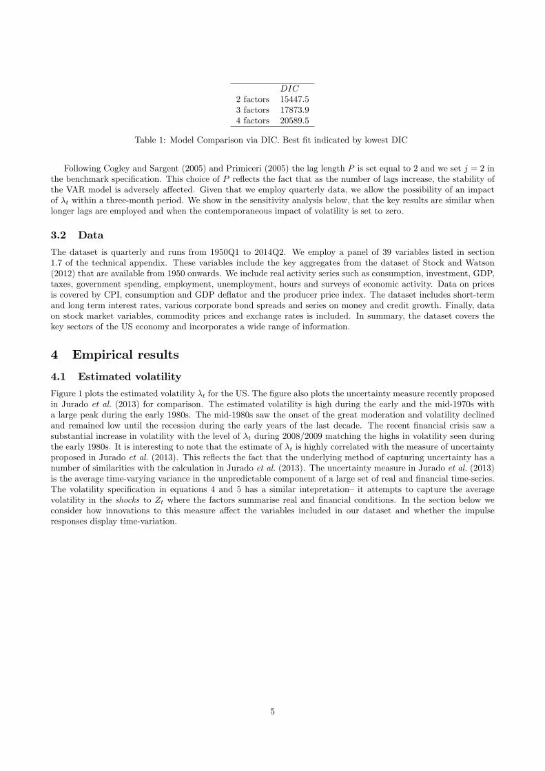
Figure 1 plots the estimated volatility λt for the US. The figure also plots the uncertainty measure recently proposedin Jurado et al. (2013) for comparison. The estimated volatility is high during the early and the mid-1970s witha large peak during the early 1980s. The mid-1980s saw the onset of the great moderation and volatility declinedand remained low until the recession during the early years of the last decade. The recent financial crisis saw asubstantial increase in volatility with the level of λt during 2008/2009 matching the highs in volatility seen duringthe early 1980s. It is interesting to note that the estimate of λt is highly correlated with the measure of uncertaintyproposed in Jurado et al. (2013). This reflects the fact that the underlying method of capturing uncertainty has anumber of similarities with the calculation in Jurado et al. (2013). The uncertainty measure in Jurado et al. (2013)is the average time-varying variance in the unpredictable component of a large set of real and financial time-series.The volatility specification in equations 4 and 5 has a similar intepretation— it attempts to capture the averagevolatility in the shocks to Zt where the factors summarise real and financial conditions. In the section below weconsider how innovations to this measure affect the variables included in our dataset and whether the impulseresponses display time-variation.

5

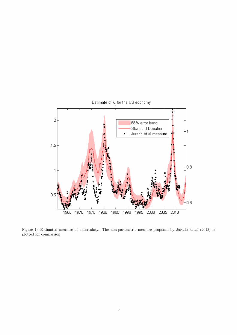
Figure 1: Estimated measure of uncertainty. The non-parametric measure proposed by Jurado et al. (2013) isplotted for comparison.

6

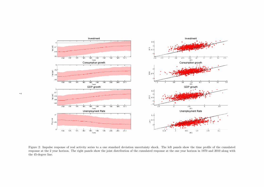
Figure 2: Impulse response of real activity series to a one standard deviation uncertainty shock. The left panels show the time profile of the cumulatedresponse at the 2 year horizon. The right panels show the joint distribution of the cumulated response at the one year horizon in 1970 and 2010 along withthe 45-degree line.

7

Figure 3: Impulse response of inflation series to a one standard deviation uncertainty shock. The left panels show the time profile of the cumulated responseat the 2 year horizon. The right panels show the joint distribution of the cumulated response at the one year horizon in 1970 and 2010 along with the45-degree line.

8

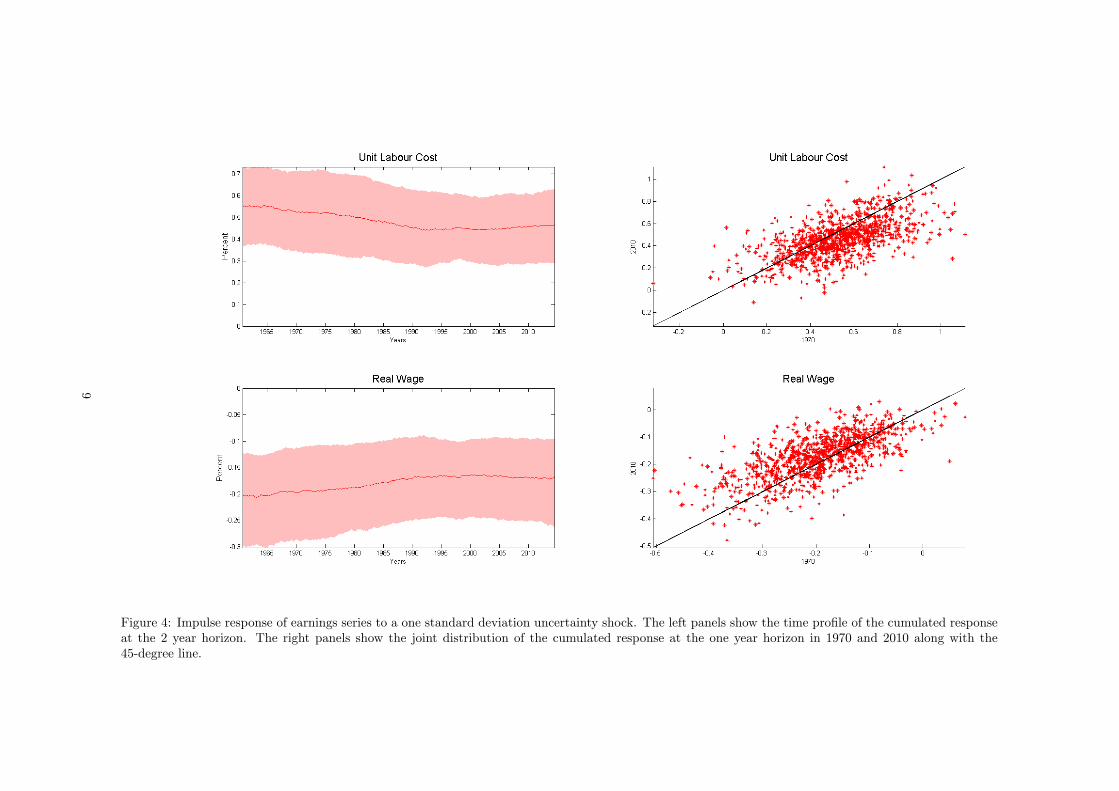
Figure 4: Impulse response of earnings series to a one standard deviation uncertainty shock. The left panels show the time profile of the cumulated responseat the 2 year horizon. The right panels show the joint distribution of the cumulated response at the one year horizon in 1970 and 2010 along with the45-degree line.

9

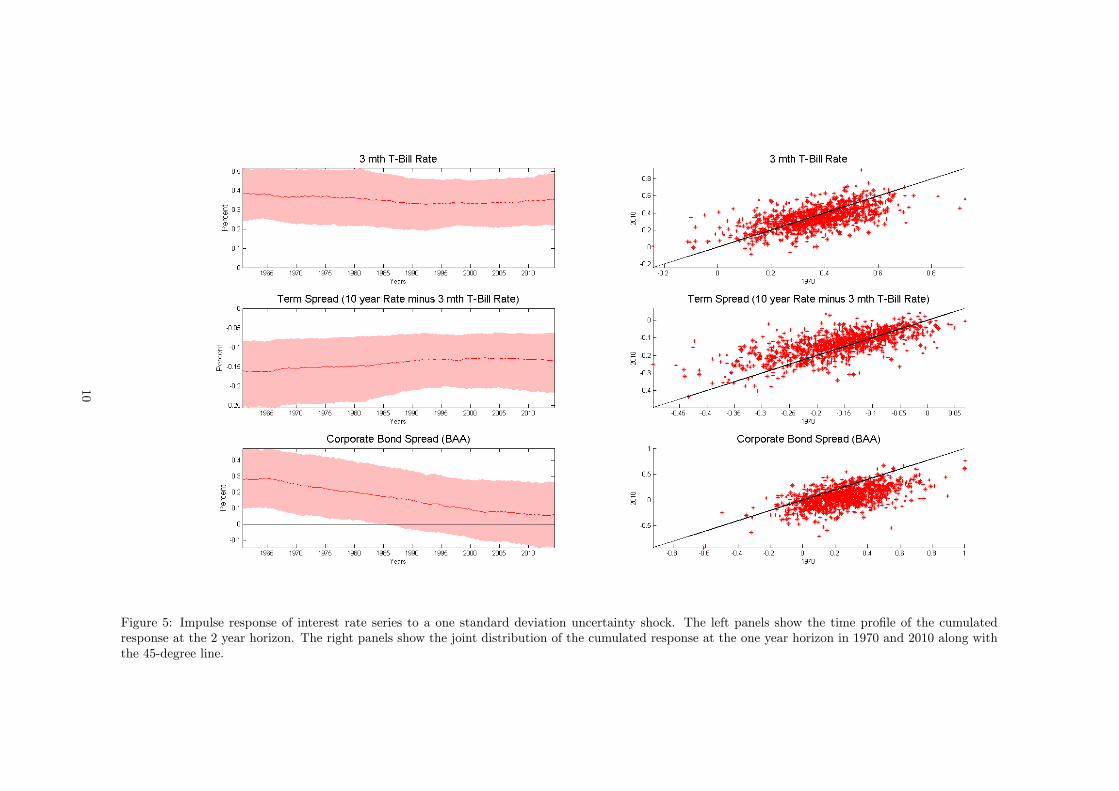
Figure 5: Impulse response of interest rate series to a one standard deviation uncertainty shock. The left panels show the time profile of the cumulatedresponse at the 2 year horizon. The right panels show the joint distribution of the cumulated response at the one year horizon in 1970 and 2010 along withthe 45-degree line.

10

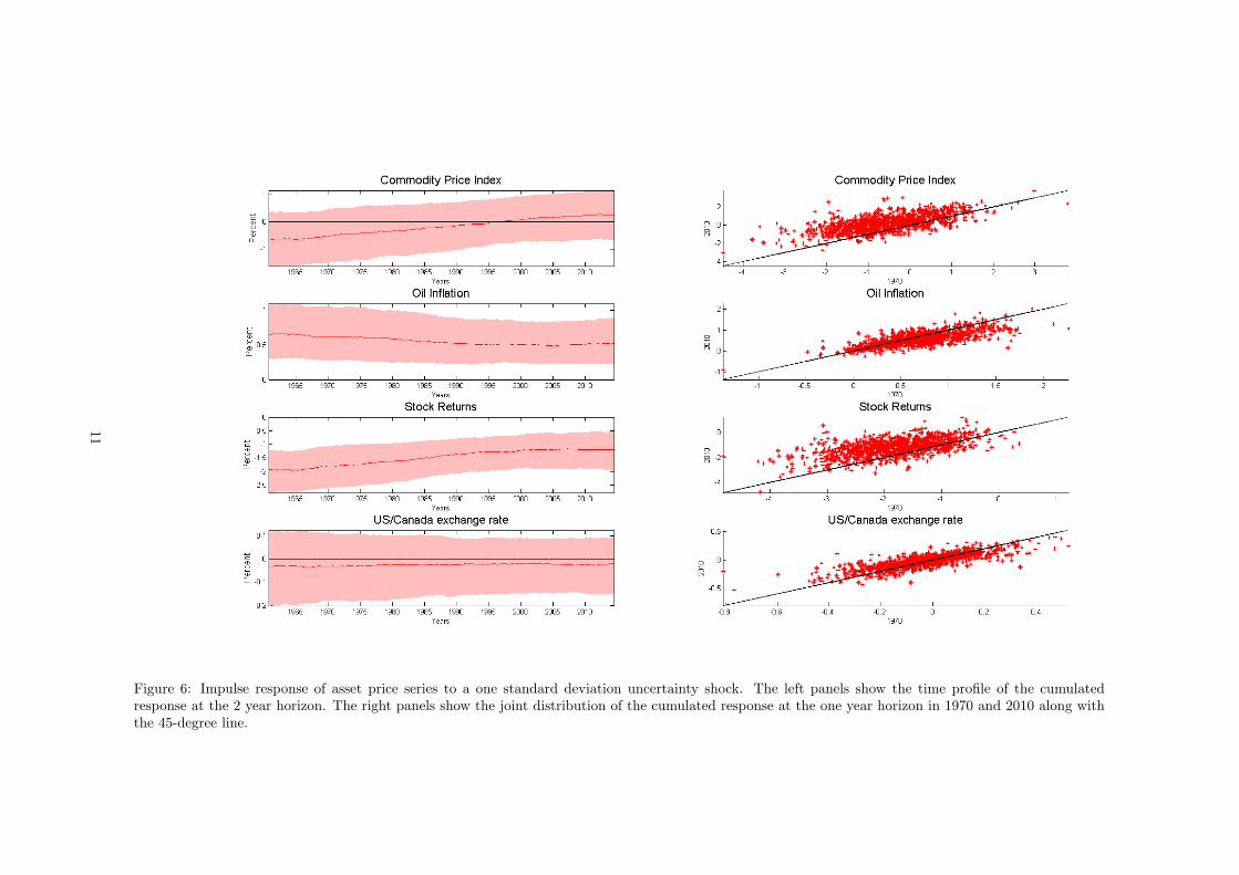
Figure 6: Impulse response of asset price series to a one standard deviation uncertainty shock. The left panels show the time profile of the cumulatedresponse at the 2 year horizon. The right panels show the joint distribution of the cumulated response at the one year horizon in 1970 and 2010 along withthe 45-degree line.

11

4.2 Impulse response to uncertainty shocks

Figure 2 shows the response of real activity variables to a 1 standard deviation positive shock to uncertainty. Theleft panels of the figure show the cumulated response at the two year horizon. The right panels display the jointdistribution of this response in the early and later part of the sample and compare this with the 45-degree line. Asystematic difference across time can be detected if the points on the scatter plot deviate from the 45-degree line.3

Figure 2 shows that the response of real activity to uncertainty has declined over time. Consider the responseof GDP growth. GDP growth fell by 0.5%-0.6% in response to the uncertainty shock over the 1970s and the early1980s. In contrast, after the mid-1990s, the decline in this variable in response to the uncertainty shock is closer to0.3%. The right panel shows that that this decline in the magnitude of the response is systematic—the points in thejoint distribution mostly lie above the 45-degree line suggesting that the response in 2010 was less negative than inthe earlier period. Similarly, the response of consumption growth, investment and the unemployment rate shows asystematic decline after the mid-1980s.Figure 3 shows the response of a number of inflation series to the uncertainty shock. Note that the response of

inflation to the uncertainty shock is estimated to be positive and thus supports the existence of pricing bias channelpostulated in Fernández-Villaverde et al. (2011). In contrast to the real activity responses, there is little evidenceof any systematic decline in the magnitude of the response. The estimated joint distribution in 1970 and 2010 isclustered evenly around the 45-degree line. Similarly figure 4 shows that a similar conclusion holds for unit labourcosts and earnings—the response of these variables is fairly stable across time.Figure 5 plots the time-varying response of the short term interest rate and spreads. While the response of the

short term rate and the the term spread is fairly constant over time, there appears to be a systematic decline inthe response of the corporate bond spread to this shock with the cumulated response falling from about 0.3% inthe early part of the sample to around 0.1% over the last decade. The bottom right panel provides some evidencethat the change in this response is systematic.The time-varying response of various asset prices to this shock is shown in figure 6. The response of stock

returns at the 2 year horizon was about -2% during the 1970s and the 1980s. In contrast, stock returns declinedby about 1% in response to the uncertainty shock after 2000. Similarly, the response of the commodity price indexhas declined over time. Note, however, that the error bands are wide for this response over the entire sample.In summary, the estimates suggest that the response of real activity indicators (GDP growth, consumption

growth, investment and unemployment) and some financial variables (corporate spread and stock returns) to un-certainty shocks has declined over time. In contrast, the the response of inflation and the short-term interest rateto this shock is estimated to have been fairly stable.We show in section 1.6 of the technical appendix that these conclusions are robust to various changes in the

specification of the empirical model. In particular, these results survive if the lag structure of the model is changed—we estimate versions of the model where (a) four lags of λt are allowed to affect the endogenous variables and (b)where the assumption that the volatility has a contemporaneous effect on the endogenous variables is relaxed. Inboth cases, we find that the response of real activity and financial variables declines while the response of inflationand the short-term rate is stable. Similarly, expanding the number of factors to 3 has little impact on theseconclusions. Finally, we employ a tighter prior on the parameters governing the degree of time-variation in thecoefficients (QB and Qλ) and find that the conclusions reached above are largely unaffected.The sensitivity analysis,therefore, supports the following main conclusion: There is evidence that the response

of real activity and some financial indicators to the uncertainty shock has declined over time. In contrast, theresponse of inflation and interest rates to this shock has remained largely stable. We now turn to a DSGE modelin order to explore the possible reasons behind the estimated temporal change in the impact of uncertainty shocks.

5 Explaining the results. A DSGE model

5.1 Summary of the model

The model used in this study is the one developed by Fernandez-Villaverde and Rubio-Ramirez (2008) (which inturn is a close relative to those developed by Christiano et al. (2005) and Smets and Wouters (2007)). FollowingChristiano et al. (2014), we augmented this model with Bernanke et al. (1999) type financial frictions. Briefly, themodel features risk-averse consumers who supply labour to differentiated and sticky wage labour unions. There arerisk-neutral entrepreneurs who borrow from perfectly competitive banks, build capital goods that they rent to the

3We focus on the two year horizon for simplicity. The full three-dimensional plots of the time-varying impulse responses can befound in the appendix to the paper.

12

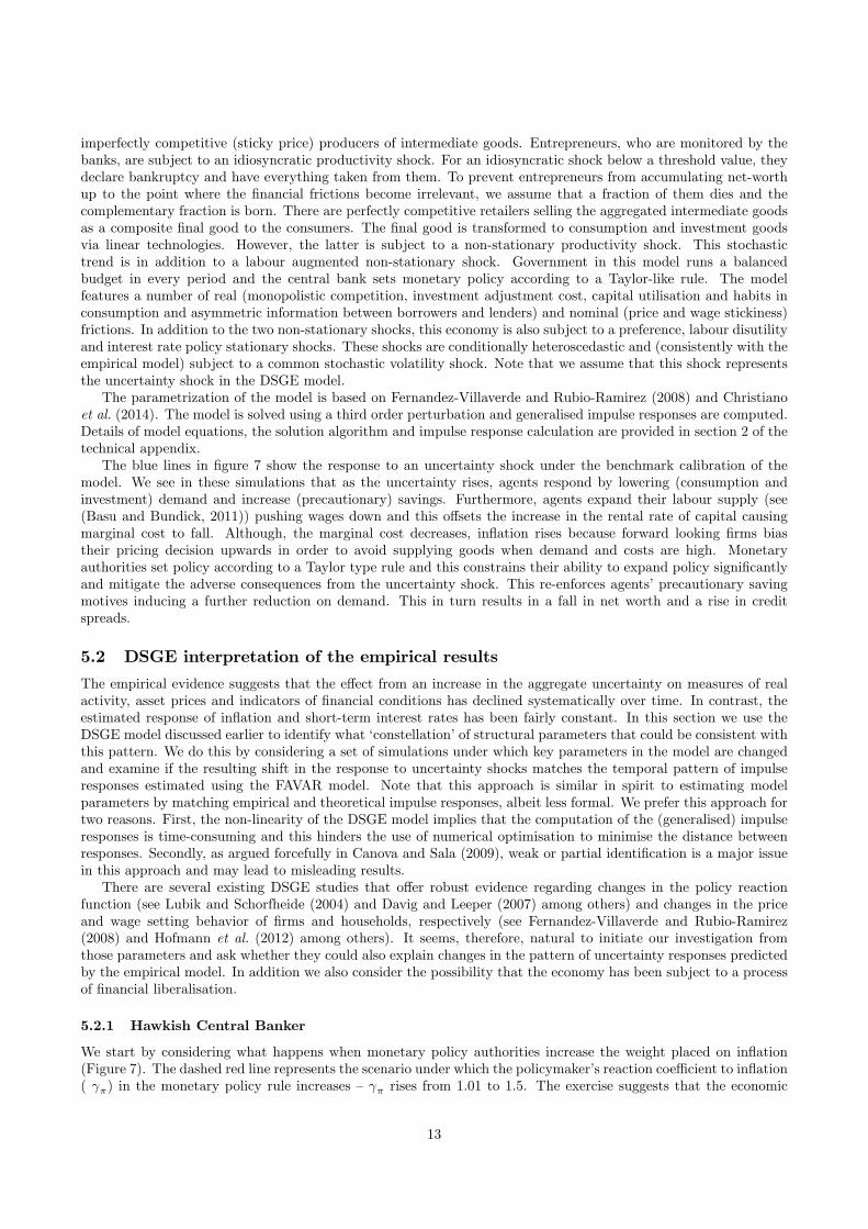
imperfectly competitive (sticky price) producers of intermediate goods. Entrepreneurs, who are monitored by thebanks, are subject to an idiosyncratic productivity shock. For an idiosyncratic shock below a threshold value, theydeclare bankruptcy and have everything taken from them. To prevent entrepreneurs from accumulating net-worthup to the point where the financial frictions become irrelevant, we assume that a fraction of them dies and thecomplementary fraction is born. There are perfectly competitive retailers selling the aggregated intermediate goodsas a composite final good to the consumers. The final good is transformed to consumption and investment goodsvia linear technologies. However, the latter is subject to a non-stationary productivity shock. This stochastictrend is in addition to a labour augmented non-stationary shock. Government in this model runs a balancedbudget in every period and the central bank sets monetary policy according to a Taylor-like rule. The modelfeatures a number of real (monopolistic competition, investment adjustment cost, capital utilisation and habits inconsumption and asymmetric information between borrowers and lenders) and nominal (price and wage stickiness)frictions. In addition to the two non-stationary shocks, this economy is also subject to a preference, labour disutilityand interest rate policy stationary shocks. These shocks are conditionally heteroscedastic and (consistently with theempirical model) subject to a common stochastic volatility shock. Note that we assume that this shock representsthe uncertainty shock in the DSGE model.The parametrization of the model is based on Fernandez-Villaverde and Rubio-Ramirez (2008) and Christiano

et al. (2014). The model is solved using a third order perturbation and generalised impulse responses are computed.Details of model equations, the solution algorithm and impulse response calculation are provided in section 2 of thetechnical appendix.The blue lines in figure 7 show the response to an uncertainty shock under the benchmark calibration of the

model. We see in these simulations that as the uncertainty rises, agents respond by lowering (consumption andinvestment) demand and increase (precautionary) savings. Furthermore, agents expand their labour supply (see(Basu and Bundick, 2011)) pushing wages down and this offsets the increase in the rental rate of capital causingmarginal cost to fall. Although, the marginal cost decreases, inflation rises because forward looking firms biastheir pricing decision upwards in order to avoid supplying goods when demand and costs are high. Monetaryauthorities set policy according to a Taylor type rule and this constrains their ability to expand policy significantlyand mitigate the adverse consequences from the uncertainty shock. This re-enforces agents’ precautionary savingmotives inducing a further reduction on demand. This in turn results in a fall in net worth and a rise in creditspreads.

5.2 DSGE interpretation of the empirical results

The empirical evidence suggests that the effect from an increase in the aggregate uncertainty on measures of realactivity, asset prices and indicators of financial conditions has declined systematically over time. In contrast, theestimated response of inflation and short-term interest rates has been fairly constant. In this section we use theDSGE model discussed earlier to identify what ‘constellation’ of structural parameters that could be consistent withthis pattern. We do this by considering a set of simulations under which key parameters in the model are changedand examine if the resulting shift in the response to uncertainty shocks matches the temporal pattern of impulseresponses estimated using the FAVAR model. Note that this approach is similar in spirit to estimating modelparameters by matching empirical and theoretical impulse responses, albeit less formal. We prefer this approach fortwo reasons. First, the non-linearity of the DSGE model implies that the computation of the (generalised) impulseresponses is time-consuming and this hinders the use of numerical optimisation to minimise the distance betweenresponses. Secondly, as argued forcefully in Canova and Sala (2009), weak or partial identification is a major issuein this approach and may lead to misleading results.There are several existing DSGE studies that offer robust evidence regarding changes in the policy reaction

function (see Lubik and Schorfheide (2004) and Davig and Leeper (2007) among others) and changes in the priceand wage setting behavior of firms and households, respectively (see Fernandez-Villaverde and Rubio-Ramirez(2008) and Hofmann et al. (2012) among others). It seems, therefore, natural to initiate our investigation fromthose parameters and ask whether they could also explain changes in the pattern of uncertainty responses predictedby the empirical model. In addition we also consider the possibility that the economy has been subject to a processof financial liberalisation.

5.2.1 Hawkish Central Banker

We start by considering what happens when monetary policy authorities increase the weight placed on inflation(Figure 7). The dashed red line represents the scenario under which the policymaker’s reaction coefficient to inflation( γπ) in the monetary policy rule increases — γπ rises from 1.01 to 1.5. The exercise suggests that the economic

13

effects of an exogenous increase in uncertainty diminish as the policymaker fights inflation aggressively. When γπrises and authorities react strongly to inflation, future inflation is expected to be on target. This reduces firms’concerns about expected inflation and makes them less forward looking. In other words, the pricing bias decreasesand the link between inflation and marginal cost is renewed. In this case authorities are able to cut the policy rateby more and for a longer period, which helps them to address the adverse effects from elevated uncertainty. Theresulting amelioration in the fall in investment improves the entrepreneurs’ leverage position and the increase inthe credit spread is smaller.The changes in the impulse responses predicted by the rise in γπ go in the direction of the empirical results—

the fall in the magnitude of the real activity and credit spread response is consistent with the estimates from theFAVAR. Note, however, that unlike the empirical estimates, the model simulations also predicts a decline in theresponse of inflation and the policy rate at all horizons.

14

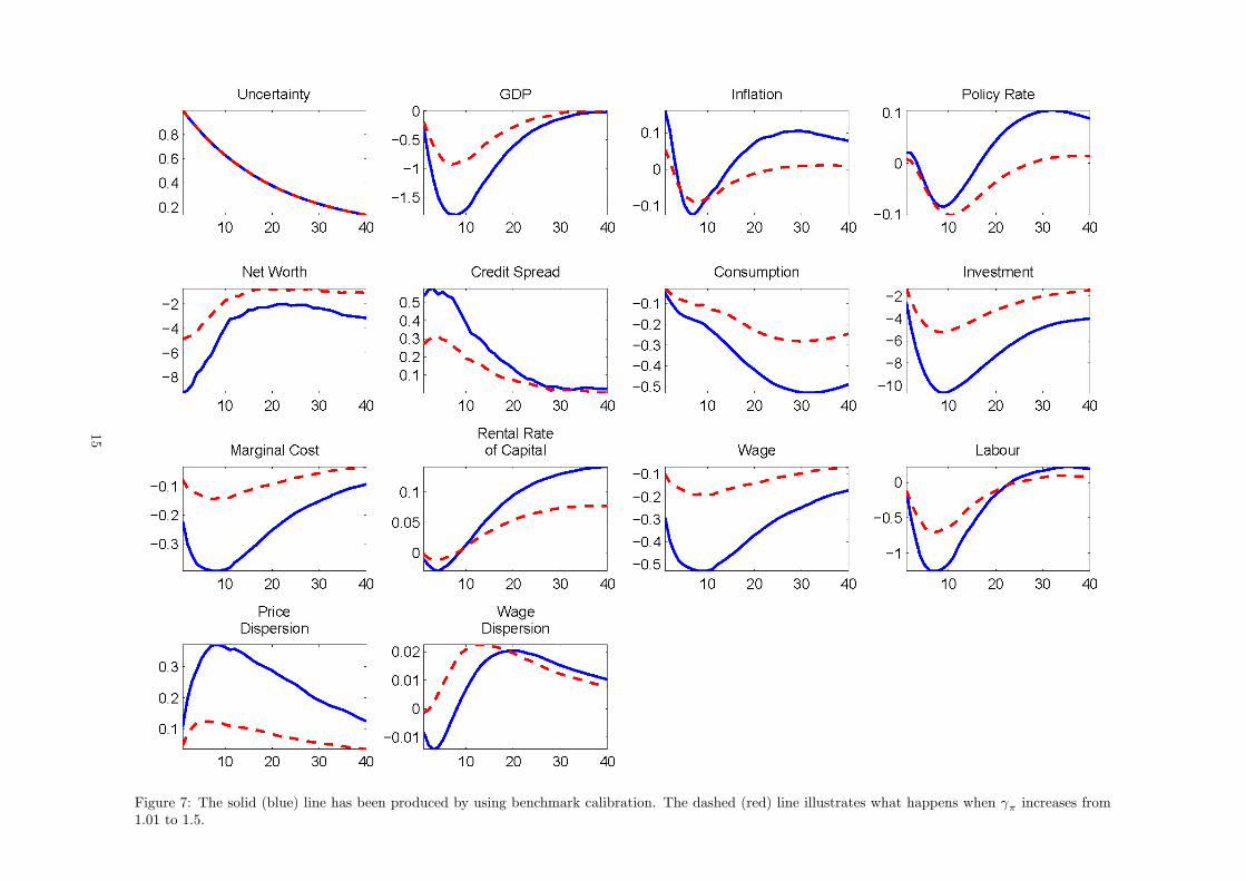
Figure 7: The solid (blue) line has been produced by using benchmark calibration. The dashed (red) line illustrates what happens when γπ increases from1.01 to 1.5.

15

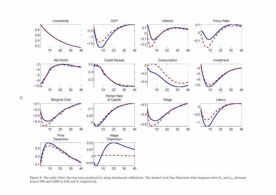
Figure 8: The solid (blue) line has been produced by using benchmark calibration. The dashed (red) line illustrates what happens when θw and χw decreasefrom 0.700 and 0.800 to 0.05 and 0, respectively.

16

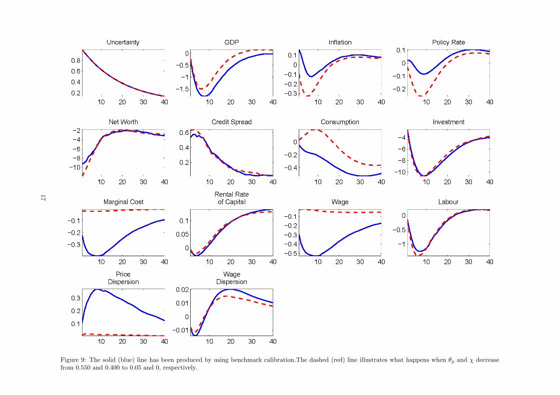
Figure 9: The solid (blue) line has been produced by using benchmark calibration.The dashed (red) line illustrates what happens when θp and χ decreasefrom 0.550 and 0.400 to 0.05 and 0, respectively.

17

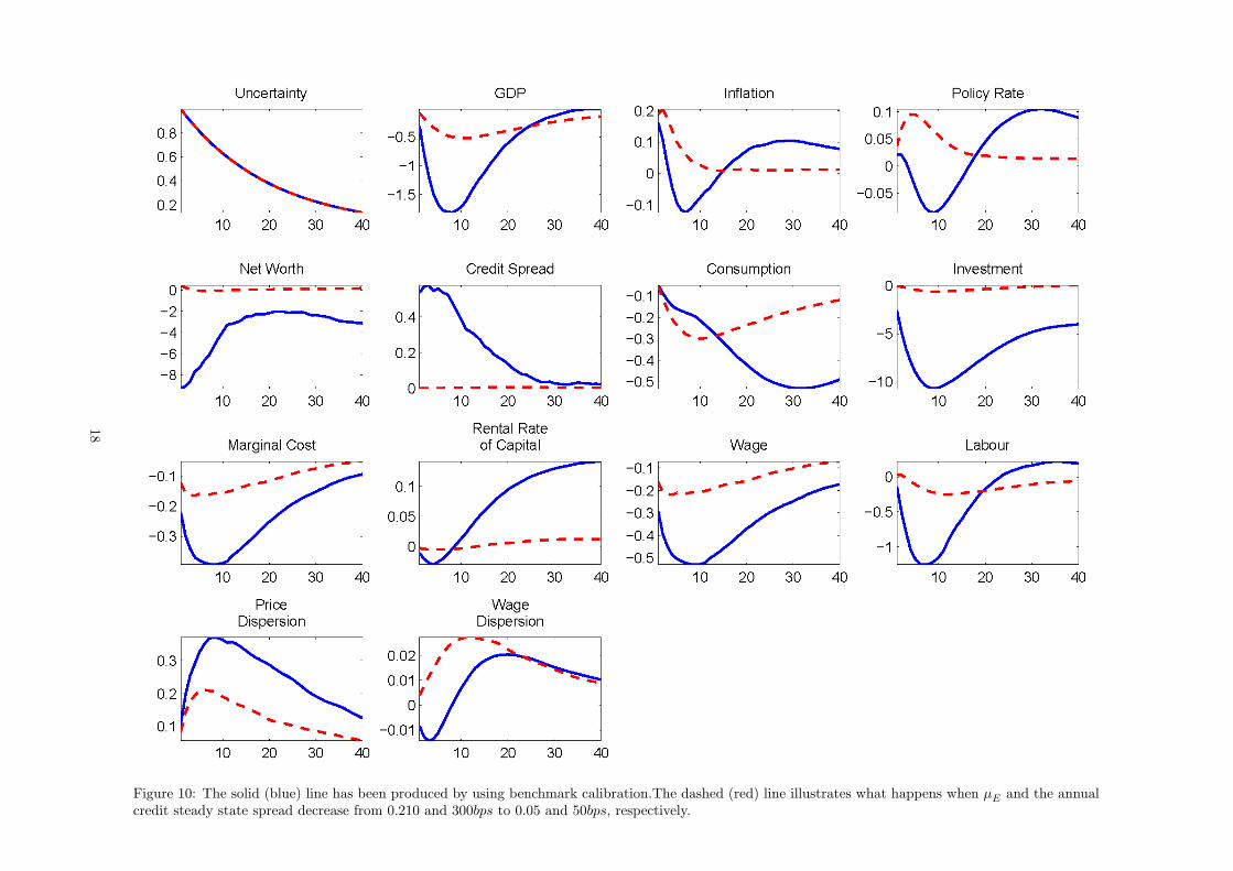
Figure 10: The solid (blue) line has been produced by using benchmark calibration.The dashed (red) line illustrates what happens when μE and the annualcredit steady state spread decrease from 0.210 and 300bps to 0.05 and 50bps, respectively.

18

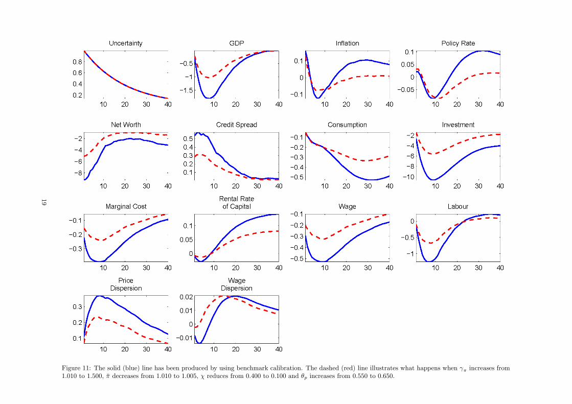
Figure 11: The solid (blue) line has been produced by using benchmark calibration. The dashed (red) line illustrates what happens when γπ increases from1.010 to 1.500, π decreases from 1.010 to 1.005, χ reduces from 0.400 to 0.100 and θp increases from 0.550 to 0.650.

19

5.2.2 Flexible Wages or prices

Next we study the effects on the economy after an uncertainty shock when nominal wages are not subject to frictions(Figure 8 ). This simulation assumes that the Calvo probability of re-setting wages θw and the wage indexationparameter χw decrease from 0.700 and 0.800 to 0.05 and 0, respectively. Relative to the benchmark case we see thatflexible wages do not lead to large changes in the impact of uncertainty on aggregate demand. Agents in the flexiblewage case respond by supplying more labour causing wages to fall by more. This turns out to have an impact onthe marginal cost and inflation as they fall in the first two years by more in the flexible wage case. However, thepricing bias channel is still present—inflation does not fall as much as the marginal cost and after two years inflationresponse closely tracks the benchmark inflation profile. This implies positive policy rates for a large period thatoffset the majority of the short lasting stimulus (via negative short term rates) and explain why demand contractsby a very similar amount under both scenarios.Following Christiano et al. (2010) we investigate the economic effects after an uncertainty shock when prices are

able to adjust freely (Figure 9)— the Calvo probability θp and indexation χ decrease from 0.550 and 0.400 to 0.05and 0, respectively. Although the effects on (aggregate) demand and prices appear to be very similar to the flexiblewages case, the transmission mechanism is very different. With flexible prices, the prices Philips curve drops fromthe system and real wages equal zero for all t. Thus price inflation becomes a function of the nominal wage inflationand not a function of the marginal cost. Given that real wages equal zero for all t, nominal wage inflation is just afunction of the real marginal cost of work (namely consumption and labour demand) which is falling.

The change in real activity response implied by these simulations is consistent with what we find using theFAVAR model. Note, however, that these experiments suggest that an increase in wage or price flexibility haslittle impact on the magnitude of the credit spread response and leads to a change in the inflation response. Thetime-varying FAVAR responses offer little evidence to support these changes.

5.2.3 Financial liberalisation

In this simulation we assume that the asymmetry between borrower and lender has been reduced (Figure 10) — theentrepreneur auditing cost μE and the annual credit steady state spread decreases from 0.210 and 300bps to 0.05and 50bps, respectively. After this change in these parameters, an uncertainty shock has almost no effect on creditspreads and net-worth. This is due to the low value of entrepreneur auditing cost (μE = 0 implies no asymmetrybetween borrowers and lenders). As a consequence, investment does not collapse in this case as agents face a tinyexternal finance premium. Note also that the dynamics of inflation and the policy rate are quite different underfinancial liberalisation and this feature does not match the FAVAR results.

5.3 Discussion

The simulations presented above indicate that the estimated changes in the response of real activity and creditspreads to uncertainty shocks can be consistent with a shift in Taylor rule parameters, wage/price rigidity andeasing of financial frictions. In contrast, it seems harder to replicate closely the empirical result that the responseof inflation and the short-term rate has been stable over time. Comparing figures 7 to 10, it appears that onecan get closest to the empirical results by increasing γπ from 1.010 to 1.500. While, the increase in the FederalReserve’s anti-inflationary stance after the mid-1980s has been documented and supported by several studies (seeLubik and Schorfheide (2004)), it seems reasonable to suppose that the US economy has been subject to otherstructural changes at the same time. For example, using a time-varying DSGE model, Fernandez-Villaverde andRubio-Ramirez (2008) provide evidence for a decrease in the inflation target and the ‘flattening’ of the Phillipscurve on top of an increase in the Taylor rule inflation coefficient.In figure 11 we consider changes in a number of parameters that match the findings of Fernandez-Villaverde and

Rubio-Ramirez (2008). In particular, this figure compares the benchmark impulse responses from those obtainedunder the scenario where monetary authorities fight inflation more aggressively (γπ increases from 1.010 to 1.500),the steady-state inflation is reduced (π decreases from 4% to 2%), firm rely less on indexation rules of thumb (χreduces from 0.400 to 0.100) and reset prices less frequently due to price stability (θp increases from 0.550 to 0.650).Figure 11 shows that the changes in the impulse responses are close to the empirical results. Under the alternativescenario, the response of real activity and spreads to the uncertainty shocks is weaker. However, the responseof inflation and the short-term interest rate is fairly similar, especially at short and medium term horizons. Theincrease in price stickiness and a decrease in indexation has an upward effect on the pricing bias which counteractsthe decrease in this channel induced by the rise in γπ. With inflation closer to a lower target, firms find it optimal

20

not to rest prices very often. However, this reduction in price re-setting leads them to account more for the risk ofbeing locked in a contractual agreement to supply goods at a price lower than the aggregate price.In contrast, a combination of financial liberalisation and changes in the Phillips curve parameters outlined above

would lead to large changes in the inflation and the interest rate response. Notice from figure 10 that as financialfrictions ease, the response of inflation to uncertainty shock is larger in magnitude. This channel is further magnifiedwith a fall in indexation and an increase in price stickiness.

Therefore, a change in Taylor rule and Phillips curve parameters provides a candidate explanation for thetemporal shift in the responses estimated using the FAVAR model. As noted above, the fact that the change inthese model parameters has been reported by other studies provides an argument for believing this explanation tobe a plausible one.

6 Conclusions

This paper considers whether the impact of uncertainty shocks on the US economy has changed over time. Usingan extended FAVAR model that allows the estimation of the time-varying impact of uncertainty shocks we findthat the response of real activity series such as GDP growth and financial series such as the BAA credit spreadto this shock has declined over time. In contrast, the estimated response of inflation and short-term interest rateshas remained fairly constant over time. We use a non-linear DSGE model with stochastic volatility to gauge thepossible factors behind these changes. The DSGE simulations suggest that the empirical results can be closelyreplicated when we incorporate an increase in the monetary authorities anti-inflation stance and simultaneouslyallow the degree of price stickiness to rise and indexation to fall. This highlights the importance of monetary policyand inflation dynamics in determining the role played by uncertainty and the importance of this shock for economicfluctuations.

References

Alessandri, Piergiorgio and Haroon Mumtaz, 2014, Financial Regimes and Uncertainty Shocks, Working Papers729, Queen Mary University of London, School of Economics and Finance.

Aruoba, Boragan, Luigi Bocola and Frank Schorfheide, 2011, A New Class of Nonlinear Times Series Models forthe Evaluation of DSGE Models, In progress.

Asai, Manabu and Michael McAleer, 2009, Multivariate stochastic volatility, leverage and news impact surfaces,Econometrics Journal 12(2), 292—309.

Basu, Susanto and Brent Bundick, 2011, Uncertainty Shocks in a Model of Effective Demand, Boston CollegeWorking Papers in Economics 774, Boston College Department of Economics.

Beetsma, Roel and Massimo Giuliodori, 2012, The changing macroeconomic response to stock market volatilityshocks, Journal of Macroeconomics 34(2), 281 — 293.

Benati, Luca, 2014, Economic Policy Uncertainty and the great recession, mimeo, University of Bern.

Bernanke, B. S., J. Boivin and P. Eliasz, 2005, Measuring the Effects of Monetary Policy: A Factor AugmentedVector Autoregressive (FAVAR) Approach, Quarterly Journal of Economics 120, 387—422.

Bernanke, Ben S., Mark Gertler and Simon Gilchrist, 1999, The financial accelerator in a quantitative businesscycle framework, in J. B. Taylor and M. Woodford (editors), Handbook of Macroeconomics, Vol. 1 of Handbookof Macroeconomics, chapter 21, pp. 1341—1393.

Berument, Hakan, Yeliz Yalcin and Julide Yildirim, 2009, The effect of inflation uncertainty on inflation: stochasticvolatility in mean model within a dynamic framework, Economic Modelling 26(6), 1,201—07.

Bloom, Nicholas, 2009, The Impact of Uncertainty Shocks, Econometrica 77(3), 623—85.

Caggiano, Giovanni, Efrem Castelnuovo and Nicolas Groshenny, 2014, Uncertainty shocks and unemployment dy-namics in U.S. recessions, Journal of Monetary Economics 67(0), 78 — 92.

21

Canova, Fabio and Luca Sala, 2009, Back to square one: Identification issues in {DSGE} models, Journal ofMonetary Economics 56(4), 431 — 449.

Carlin, Bradley P., Nicholas G. Polson and David S. Stoffer, 1992, A Monte Carlo Approach to Nonnormal andNonlinear State-Space Modeling, Journal of the American Statistical Association 87(418), 493—500.

Carriero, Andrea, Todd Clark and Massimiliano Marcellino, 2012, Common Drifting Volatility in Large BayesianVARs, CEPR Discussion Papers 8894, C.E.P.R. Discussion Papers.

Carter, C and P Kohn, 2004, On Gibbs sampling for state space models, Biometrika 81, 541—53.

Christiano, Lawrence, Cosmin L. Ilut, Roberto Motto and Massimo Rostagno, 2010, Monetary Policy and StockMarket Booms, NBER Working Papers 16402, National Bureau of Economic Research, Inc.

Christiano, Lawrence, Martin Eichenbaum and Charles Evans, 2005, Nominal Rigidities and the Dynamic Effectsof a shock to Monetary Policy, Journal of Political Economy 113, 1—45.

Christiano, Lawrence, Roberto Motto and Massimo Rostagno, 2014, Risk Shocks, American Economic Review104(1), 27—65.

Cogley, T. and T. J. Sargent, 2005, Drifts and Volatilities: monetary policies and outcomes in the Post WWII U.S.,Review of Economic Dynamics 8, 262—302.

Davig, Troy and Eric M. Leeper, 2007, Generalizing the Taylor Principle, American Economic Review 97(3), 607—635.

Delnegro, Marco and Christopher Otrok, 2005, Dynamic factor models with time-varying parameters, Mimeo,Federal Reserve Bank of Atlanta.

Fernandez-Villaverde, Jesus and Juan F. Rubio-Ramirez, 2008, How Structural Are Structural Parameters?, NBERMacroeconomics Annual 2007, Volume 22, NBER Chapters, National Bureau of Economic Research, Inc, pp. 83—137.

Fernandez-Villaverde, Jesus, Pablo Guerron-Quintana, Juan F. Rubio-Ramirez and Martin Uribe, 2011, Risk Mat-ters: The Real Effects of Volatility Shocks, American Economic Review 101(6), 2530—61.

Fernández-Villaverde, Jesús, Pablo A. Guerrón-Quintana, Keith Kuester and Juan Rubio-Ramírez, 2011, FiscalVolatility Shocks and Economic Activity, NBER Working Papers 17317, National Bureau of Economic Research,Inc.

Hofmann, Boris, Gert Peersman and Roland Straub, 2012, Time variation in U.S. wage dynamics, Journal ofMonetary Economics 59(8), 769—783.

Jacquier, E, N Polson and P Rossi, 1994, Bayesian analysis of stochastic volatility models, Journal of Business andEconomic Statistics 12, 371—418.

Jurado, Kyle, Sydney C. Ludvigson and Serena Ng, 2013, Measuring Uncertainty, NBER Working Papers 19456,National Bureau of Economic Research, Inc.

Koop, Gary and Simon M. Potter, 2011, Time varying {VARs} with inequality restrictions, Journal of EconomicDynamics and Control 35(7), 1126 — 1138.

Koopman, Siem Jan and Eugenie Hol Uspensky, 2000, The Stochastic Volatility in Mean Model, Tinbergen InstituteDiscussion Paper 00-024/4, Tinbergen Institute.

Kwiatkowski, Lukasz, 2010, Markov Switching In-Mean Effect. Bayesian Analysis in Stochastic Volatility Frame-work, Central European Journal of Economic Modelling and Econometrics 2(1), 59—94.

Lemoine, M. and C. Mougin, 2010, The Growth-Volatility Relationship: new Evidence Based on Stochastic Volatilityin Mean Models, Working Paper 285, Banque de France.

Lubik, Thomas A. and Frank Schorfheide, 2004, Testing for Indeterminacy: An Application to U.S. MonetaryPolicy, American Economic Review 94(1), 190—217.

22

Mumtaz, Haroon and Konstantinos Theodoridis, n.d., The international transmission of volatility shocks: an em-pirical analysis, Journal of European Economic Association .

Primiceri, G, 2005, Time varying structural vector autoregressions and monetary policy, The Review of EconomicStudies 72(3), 821—52.

Smets, Frank and Rafael Wouters, 2007, Shocks and Frictions in US Business Cycles: a Bayesian DSGE Approach,American Economic Review 97, 586—606.

Spiegelhalter, David J., Nicola G. Best, Bradley P. Carlin and Angelika Van Der Linde, 2002, Bayesian measures ofmodel complexity and fit, Journal of the Royal Statistical Society: Series B (Statistical Methodology) 64(4), 583—639.

Stock, James H. and Mark W.Watson, 2012, Generalized Shrinkage Methods for Forecasting Using Many Predictors,Journal of Business & Economic Statistics 30(4), 481—493.

Watson, Mark W., 2014, Inflation Persistence, the NAIRU, and the Great Recession, American Economic Review104(5), 31—36.

23

The changing transmission of uncertainty shocks in the US: anempirical analysis (Technical Appendix)∗

Haroon Mumtaz† Konstantinos Theodoridis‡

December 10, 2014

Abstract

Technical Appendix

1 Estimation of the FAVAR model

The TVP VAR model is defined as

Zt = ct +P∑j=1

βtjZt−j +J∑j=0

γtj lnλt−j +Ω1/2t et (1)

where Zt is a matrix of endogenous variables describe below.

B = vec([c;β;λ]) (2)

Bt = Bt−1 + ηt, V AR (ηt) = QB

Ωt = A−1t HtA

−1′t

where At is lower triangular. Each non-zero element of At evolves as a random walk

at = at−1 + gt, V AR(gt) = G (3)

where G is block diagonal as in Primiceri (2005).Following Carriero et al. (2012) the volatility process is defined as

Ht = λtS (4)

S = diag(s1, .., sN )

The overall volatility evolves as an AR(1) process

lnλt = α+ F lnλt−1 + ηt, V AR(ηt) = Qλ (5)

1.1 Priors and Starting values

1.1.1 Factors

We use a principal component estimator to calculate an initial value for the factors Zt. The initial conditions for

the Kalman filter employed in the Carter and Kohn (2004) step are set as Z0˜N(Z1, I

).

∗The views expressed in this paper are those of the authors, and not necessarily those of the Bank of England.†Queen Mary College. Email: h.mumtaz@qmul.ac.uk‡Bank of England. Email: Konstantinos.Theodoridis@bankofengland.co.uk

1

1.1.2 Factor Loadings and error variances

The initial conditions for the factor loadings are obtained via an OLS estimate of the factor loadings using the first 40observations of the sample period and employing the principal components Zt. Let Λols denote the OLS estimate ofthe factor loadings estimated using the pre-sample data described above. The prior is set as Λ0˜N(Λols, var(Λols)).The prior on QΛ is assumed to be inverse Wishart QΛ,0 ∼ IW

(QΛ,0, T0

)where QΛ,0 is assumed to be T0 ×

var(Λols)× 10−4 × 3.5 and T0 is the length of the sample used to for calibration. This follows Cogley and Sargent(2005).The prior for the diagonal elements of R is assumed to be IG (R0, VR) where the scale parameter R0 = 0.001

and VR = 5.

1.1.3 VAR Coefficients

The initial conditions for the VAR coefficients B0 are obtained via an OLS estimate of a fixed coefficient VARusing the first 40 observations of the sample period. The VAR is estimated using the principal components Zt.Let Bolsand vols denote the OLS estimate of the VAR coefficients and the covariance matrix estimated on thepre-sample data described above. The prior for B0˜N(Bols, var(Bols)). The prior on QB is assumed to be inverseWishart QB,0 ∼ IW

(QB,0, T0

)where QB,0 is assumed to be T0 × var(Bols) × 10−4 × 3.5 and T0 is the length of

the sample used to for calibration.

1.1.4 Elements of the A matrix

The prior for the off-diagonal elements At is A0 ∼ N(aols, V

(aols

))where aols are the off-diagonal elements of

vols, with each row scaled by the corresponding element on the diagonal. V(aols

)is assumed to be diagonal with

the elements set equal to 10 times the absolute value of the corresponding element of aols. The prior distribution forthe blocks of G is inverse Wishart: Gi,0 ∼ IW (Gi,Ki) where i = 1..N − 1 indexes the blocks of S. Gi is calibratedusing aols. Specifically, Gi is a diagonal matrix with the relevant elements of aols multiplied by 10−3.

1.1.5 Elements of S and the parameters of the transition equation

The elements of S have an inverse Gamma prior: P (si)˜IG(S0,i, V0). The degrees of freedom V0 are set equal to1. The prior scale parameters are set by estimating the following regression: λit = S0,iλt + εt where λt is the firstprincipal component of the stochastic volatilities λit obtained using a univariate stochastic volatility model for theresiduals of each equation of a VAR estimated via OLS using the endogenous variables Zt.

We set a normal prior for the unconditional mean μ = α1−F . This prior is N(μ0, Z0) where μ0 = 0 and

Z0 = 10.The prior for Qλ is IG (Q0, VQ0) where Q0 is the average of the variances of the transition equations ofthe initial univariate stochastic volatility estimates and VQ0 = 5. The prior for F is N (F0, L0) where F0 = 0.8 andL0 = 1.

1.1.6 Common Volatility λt

The prior for the initial value of λt is defined as lnλ0 ∼ N(lnμ0, I) where μ0 is the initial value of λt.

1.2 MCMC algorithm

The MCMC algorithm is based on drawing from the following conditional posterior distributions (Ξ denotes allother parameters):

1. G(Λt\Ξ). Given a draw for the factors the variances R and the variance of the shock to the transition equationQΛ, the following TVP regression applies for the ith Xit :

Xit = ΛitZt +R1/2i εit

Λit = Λit−1 + ηit, V AR (ηit) = QΛ,i

As this is a linear and Gaussian state space model, the Carter and Kohn (2004) algorithm can be ap-plied to draw from the conditional posterior of Λit. The distribution of the time-varying loadings condi-tional on all other parameters is linear and Gaussian: Λit\Xit,Ξ ∼ N

(ΛT\T , PT\T

)and Λt\Λt+1,Xit,Ξ ∼

N(Λt\t+1,Λt+1 , Pt\t+1,Λt+1

)where t = T − 1, ..1, Ξ denotes a vector that holds all the other VAR parameters.

2

As shown by Carter and Kohn (2004) the simulation proceeds as follows. First we use the Kalman filter todraw ΛT\T and PT\T and then proceed backwards in time using Λt|t+1,Λt+1 = Λt|t + Pt|tP

−1t+1|t

(Λt+1 − Λt|t

)and Pt|t+1,Λt+1 = Pt|t− Pt|tP−1t+1|tPt|t. Note that in order to deal rotational indeterminancy of the factors andfactor loadings, we fix the first K factor loadings where K is the number of factors. In particular, the firstK ×K block of Λit is equal to an identity matrix for all time periods (see Bernanke et al. (2005)).

2. G(QΛ,i\Ξ). Given a draw for Λit, the conditional posterior for QΛ,i is inverse Wishart with scale matrix anddegrees of freedom defined as: IW

(η′itηit + QΛ,0, T + T0

).

3. G(R\Ξ). The diagonal elements of R have an inverse Gamma conditional posterior:

G(Ri\Ξ)˜IG (ε′itεit +R0, T + VR)

4. G (Z\Ξ). Given the parameters of the observation equation (Λt, R) and the transition equation (Bt,Ωt),equations ?? and 1 constitute a linear Gaussian state space model and the Carter and Kohn (2004) algo-rithm can be employed to draw from the conditional posterior distribution of the factors. Carter and Kohn

(2004) show that the conditional posterior is defined as ZT \Xit,Ξ ∼ N(ZT\T , PT\T

)and Zt\Zt+1,Xit,Ξ ∼

N(Zt\t+1,Zt+1 , Pt\t+1,Zt+1

)where t = T − 1, ..1, Ξ denotes a vector that holds all the other VAR parameters.

A run of the Kalman filter delivers ZT\T and PT\T as the filtered states and its variance at the end of the

sample. Then one proceeds backwards in time to obtain Zt\t+1,Zt+1 = Zt|t+ Pt|tF′t P

−1t+1|t

(Zt+1 − μt − FZt|t

)and Pt|t+1,Zt+1 = Pt|t − Pt|tF ′tP−1t+1|tFtPt|t. Note that Ft and μt denote the coefficients on the lags and thecoefficients on pre-determined variables in the transition equation 1 respectively in companion form.

5. G(Bt\Ξ). Given a draw for the factors and variances Ωt, QB , 1 and 2 constitute a VAR with time-varying para-meters and the Carter and Kohn (2004) algorithm can again be applied to draw from the conditional posteriorof the VAR coefficients. The distribution of the time-varying VAR coefficients Bt conditional on all other para-meters is linear and Gaussian: Bt\Zt,Ξ ∼ N

(BT\T , PT\T

)and Bt\Bt+1,Zt,Ξ ∼ N

(Bt\t+1,Bt+1

, Pt\t+1,Bt+1

)where t = T−1, ..1, Ξ denotes a vector that holds all the other VAR parameters. As shown by Carter and Kohn(2004) the simulation proceeds as follows. First we use the Kalman filter to draw BT\T and PT\T and then pro-ceed backwards in time using Bt|t+1,Bt+1

= Bt|t+Pt|tP−1t+1|t

(Bt+1 −Bt|t

)and Pt|t+1,Bt+1

= Pt|t−Pt|tP−1t+1|tPt|t.Rejection sampling is used to ensure that the draws satisfy stability at each point in time.

6. G(QB\Ξ). The draw for QB is standard with conditional distribution IW(η′tηt + QB,0, T + T0

).

7. G(At\Ξ). Given a draw for the VAR parameters and the model can be written as A′t (vt) = et where vt denotesthe VAR residuals. This is a system of linear equations with time-varying coefficients and a known form ofheteroscedasticity. The jth equation of this system is given as vjt = −ajtv−jt + ejt where the subscript jdenotes the jth column of v while −j denotes columns 1 to j−1. Note that the variance of ejt is time-varyingand given by λtsj . The time-varying coefficient follows the process ajt = ajt−1 + gjt with the shocks tothe jth equation gjt uncorrelated with those from other equations. In other words the covariance matrixvar (g) is assumed to be block diagonal as in Primiceri (2005). With this assumption in place, the Carter andKohn (2004) algorithm can be applied to draw the time varying coefficients for each equation of this systemseperately.

8. G(S\Ξ). Given a draw for the VAR parameters the model in can be written as A′ (vt) = et. The jth equationof this system is given by vjt = −ajtv−jt + ejt where the variance of ejt is time-varying and given by λtsj .Given a draw for λt this equation can be re-written as vjt = −ajtv−jt+ ejt where vjt = vjt

λ1/2t

and the variance

of ejt is sj . The conditional posterior is for this variance is inverse Gamma with scale parameter e′jtejt + S0,jand degrees of freedom V0 + T.

9. G(λt\Ξ).Conditional on the VAR parameters, and the parameters of the transition equation, the model has amultivariate non-linear state-space representation. Carlin et al. (1992) show that the conditional distributionof the state variables in a general state-space model can be written as the product of three terms:

ht\Zt,Ξ ∝ f(ht\ht−1

)× f

(ht+1\ht

)× f

(Zt\ht,Ξ

)(6)

3

where Ξ denotes all other parameters and ht = lnλt. In the context of stochastic volatility models, Jacquieret al. (1994) show that this density is a product of log normal densities for λt and λt+1 and a normal densityfor Zt.Carlin et al. (1992) derive the general form of the mean and variance of the underlying normal density

for f(ht\ht−1, ht+1,Ξ

)∝ f

(ht\ht−1

)× f

(ht+1\ht

)and show that this is given as

f(ht\ht−1, ht+1,Ξ

)∼ N (B2tb2t, B2t) (7)

where B−12t = Q−1λ + F ′Q−1λ F and b2t = ht−1F ′Q−1λ + ht+1Q−1λ F. Note that due to the non-linearity of the

observation equation of the model an analytical expression for the complete conditional ht\Zt,Ξ is unavailableand a metropolis step is required. Following Jacquier et al. (1994) we draw from 6 using a date-by-dateindependence metropolis step using the density in 7 as the candidate generating density. This choice implies

that the acceptance probability is given by the ratio of the conditional likelihood f(Zt\ht,Ξ

)at the old and

the new draw. To implement the algorithm we begin with an initial estimate of h = ln λt We set the matrixhold equal to the initial volatility estimate. Then at each date the following two steps are implemented:

(a) Draw a candidate for the volatility hnewt using the density 6 where b2t = hnewt−1 F′Q−1λ + holdt+1Q

−1λ F and

B−12t = Q−1λ + F ′Q−1λ F

(b) Update holdt = hnewt with acceptance probabilityf(Zt\hnewt ,Ξ)f(Zt\holdt ,Ξ)

where f(Zt\ht,Ξ

)is the likelihood of the

VAR for observation t and defined as |Ωt|−0.5−0.5 exp(etΩ

−1t e′t

)where et = Zt−

(ct +

∑Pj=1 βtjZt−j +

∑Jj=0 γtj lnλt−j

and Ωt = A−1t

(exp(ht)S

)A−1

′t

Repeating these steps for the entire time series delivers a draw of the stochastic volatilties.1

7. G(α, F\Ξ).We re-write the transition equation in deviations from the mean

ht − μ = F(ht−1 − μ

)+ ηt (8)

where the elements of the mean vector μi are defined asαi1−Fi . Conditional on a draw for ht and μ the transition

equation 8 is a simply a linear regression and the standard normal and inverse Gamma conditional posteriorsapply. Consider h∗t = Fh

∗t−1+ ηt, V AR (ηt) = Qλand h

∗t = ht−μ, h∗t−1 = ht−1−μ. The conditional posterior

of F is N (θ∗, L∗) where

θ∗ =

(L−10 +

1

Qλh∗′t−1h

∗t−1

)−1(L−10 F0 +

1

Qλh∗′t−1h

∗t

)

L∗ =

(L−10 +

1

Qλh∗′t−1h

∗t−1

)−1

The conditional posterior of Qλ is inverse Gamma with scale parameter η′tηt+Q0 and degrees of freedom T + VQ0.Given a draw for F , equation 8 can be expressed as Δht = Cμ + ηt where Δht = ht − Fht−1 and C = 1 − F.

The conditional posterior of μ is N (μ∗, Z∗) where

μ∗ =

(Z−10 +

1

QλC ′C

)−1(Z−10 μ0 +

1

QλC ′Δht

)

Z∗ =

(Z−10 +

1

QλC ′C

)−1

Note that α can be recovered as μ (1− θ)1 In order to take endpoints into account, the algorithm is modified slightly for the initial condition and the last observation. Details

of these changes can be found in Jacquier et al. (1994).

4

1.3 A Monte-Carlo experiment

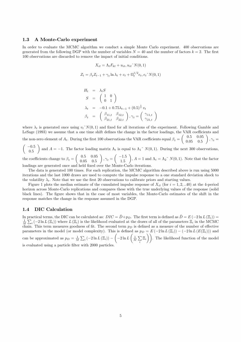
In order to evaluate the MCMC algorithm we conduct a simple Monte Carlo experiment. 400 observations aregenerated from the following DGP with the number of variables N = 40 and the number of factors k = 2. The first100 observations are discarded to remove the impact of initial conditions.

Xit = ΛtFkt + uit, uit˜N(0, 1)

Zt = βtZt−1 + γt lnλt + ct +Ω1/2t et, et˜N(0, 1)

Ht = λtS

S =

(1 00 1

)

λt = −0.1 + 0.75λt−1 + (0.5)12 vt

βt =

(β11,t β12,tβ21,t β22,t

), γt =

(γ11,tγ21,t

)

where λt is generated once using vt˜N(0, 1) and fixed for all iterations of the experiment. Following Gamble andLeSage (1993) we assume that a one time shift defines the change in the factor loadings, the VAR coefficients and

the non-zero element of At. During the first 100 observations the VAR coefficients equal βt =(0.5 0.050.05 0.5

), γt =( −0.5

0.5

)and A = −1. The factor loading matrix Λt is equal to Λ1˜ N(0, 1). During the next 300 observations,

the coefficients change to βt =(0.5 0.050.05 0.5

), γt =

( −1.51.5

), A = 1 and Λt = Λ2˜ N(0, 1). Note that the factor

loadings are generated once and held fixed over the Monte-Carlo iterations.The data is generated 100 times. For each replication, the MCMC algorithm described above is run using 5000

iterations and the last 1000 draws are used to compute the impulse response to a one standard deviation shock tothe volatility λt. Note that we use the first 20 observations to calibrate priors and starting values.Figure 1 plots the median estimate of the cumulated impulse response of Xit (for i = 1, 2, ..40) at the 4-period

horizon across Monte-Carlo replications and compares these with the true underlying values of the response (solidblack lines). The figure shows that in the case of most variables, the Monte-Carlo estimates of the shift in theresponse matches the change in the response assumed in the DGP.

1.4 DIC Calculation

In practical terms, the DIC can be calculated as: DIC = D+pD. The first term is defined as D = E (−2 lnL (Ξi)) =1M

∑i (−2 lnL (Ξi)) where L (Ξi) is the likelihood evaluated at the draws of all of the parameters Ξi in the MCMC

chain. This term measures goodness of fit. The second term pD is defined as a measure of the number of effectiveparameters in the model (or model complexity). This is defined as pD = E (−2 lnL (Ξi)) − (−2 lnL (E(Ξi))) andcan be approximated as pD = 1

M

∑i (−2 lnL (Ξi)) −

(−2 lnL

(1M

∑i

Ξi

)). The likelihood function of the model

is evaluated using a particle filter with 2000 particles.

5

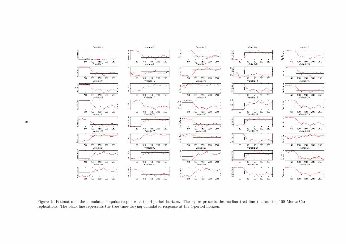
Figure 1: Estimates of the cumulated impulse response at the 4-period horizon. The figure presents the median (red line ) across the 100 Monte-Carloreplications. The black line represents the true time-varying cumulated response at the 4-period horizon.

6

1.5 Impulse responses from the benchmark model (full 3-D figures)

7

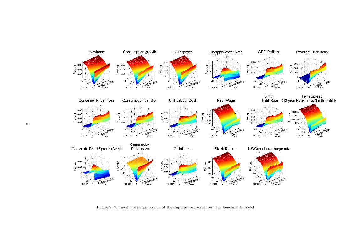
Figure 2: Three dimensional version of the impulse responses from the benchmark model

8

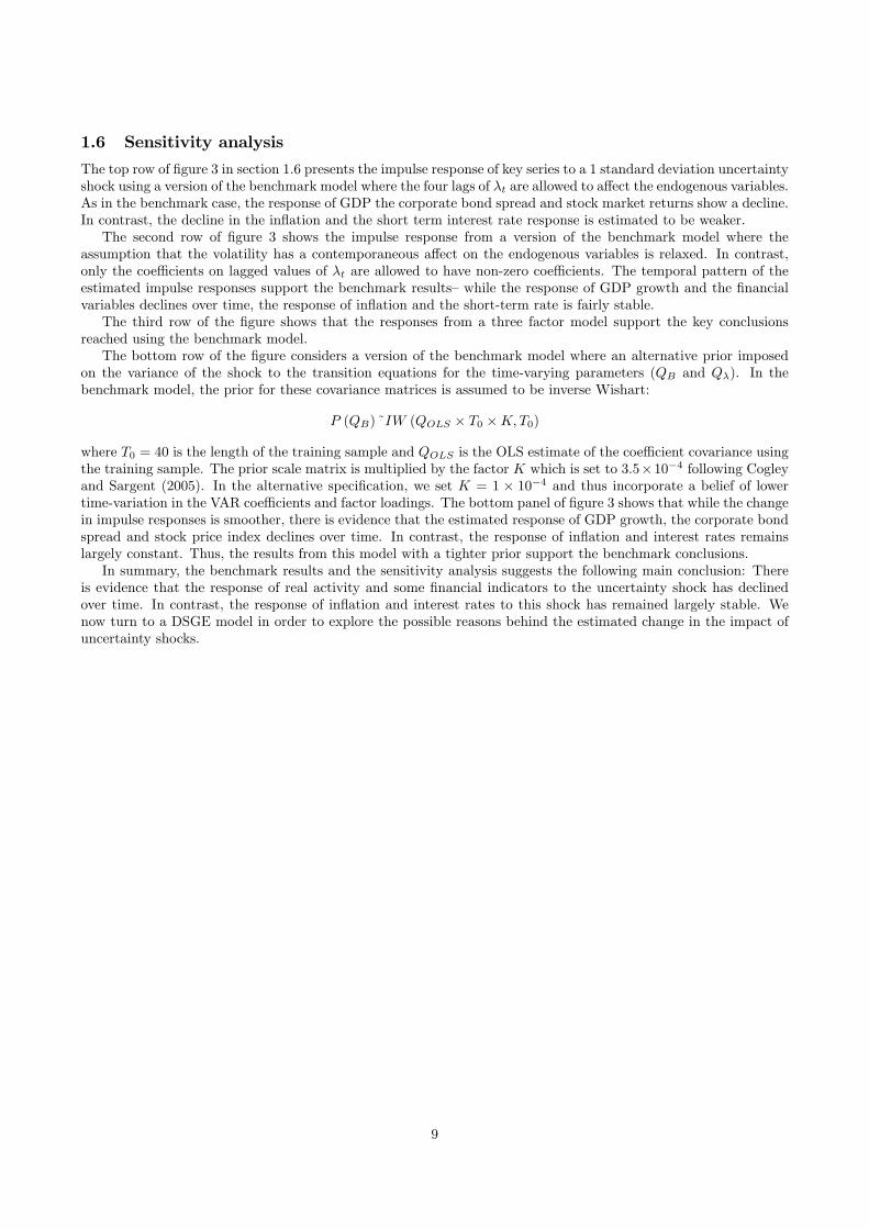
1.6 Sensitivity analysis

The top row of figure 3 in section 1.6 presents the impulse response of key series to a 1 standard deviation uncertaintyshock using a version of the benchmark model where the four lags of λt are allowed to affect the endogenous variables.As in the benchmark case, the response of GDP the corporate bond spread and stock market returns show a decline.In contrast, the decline in the inflation and the short term interest rate response is estimated to be weaker.The second row of figure 3 shows the impulse response from a version of the benchmark model where the

assumption that the volatility has a contemporaneous affect on the endogenous variables is relaxed. In contrast,only the coefficients on lagged values of λt are allowed to have non-zero coefficients. The temporal pattern of theestimated impulse responses support the benchmark results— while the response of GDP growth and the financialvariables declines over time, the response of inflation and the short-term rate is fairly stable.The third row of the figure shows that the responses from a three factor model support the key conclusions

reached using the benchmark model.The bottom row of the figure considers a version of the benchmark model where an alternative prior imposed

on the variance of the shock to the transition equations for the time-varying parameters (QB and Qλ). In thebenchmark model, the prior for these covariance matrices is assumed to be inverse Wishart:

P (QB) ˜IW (QOLS × T0 ×K,T0)

where T0 = 40 is the length of the training sample and QOLS is the OLS estimate of the coefficient covariance usingthe training sample. The prior scale matrix is multiplied by the factor K which is set to 3.5×10−4 following Cogleyand Sargent (2005). In the alternative specification, we set K = 1 × 10−4 and thus incorporate a belief of lowertime-variation in the VAR coefficients and factor loadings. The bottom panel of figure 3 shows that while the changein impulse responses is smoother, there is evidence that the estimated response of GDP growth, the corporate bondspread and stock price index declines over time. In contrast, the response of inflation and interest rates remainslargely constant. Thus, the results from this model with a tighter prior support the benchmark conclusions.In summary, the benchmark results and the sensitivity analysis suggests the following main conclusion: There

is evidence that the response of real activity and some financial indicators to the uncertainty shock has declinedover time. In contrast, the response of inflation and interest rates to this shock has remained largely stable. Wenow turn to a DSGE model in order to explore the possible reasons behind the estimated change in the impact ofuncertainty shocks.

9

Figure 3: Sensitivity Analysis

10

1.7 Data

11

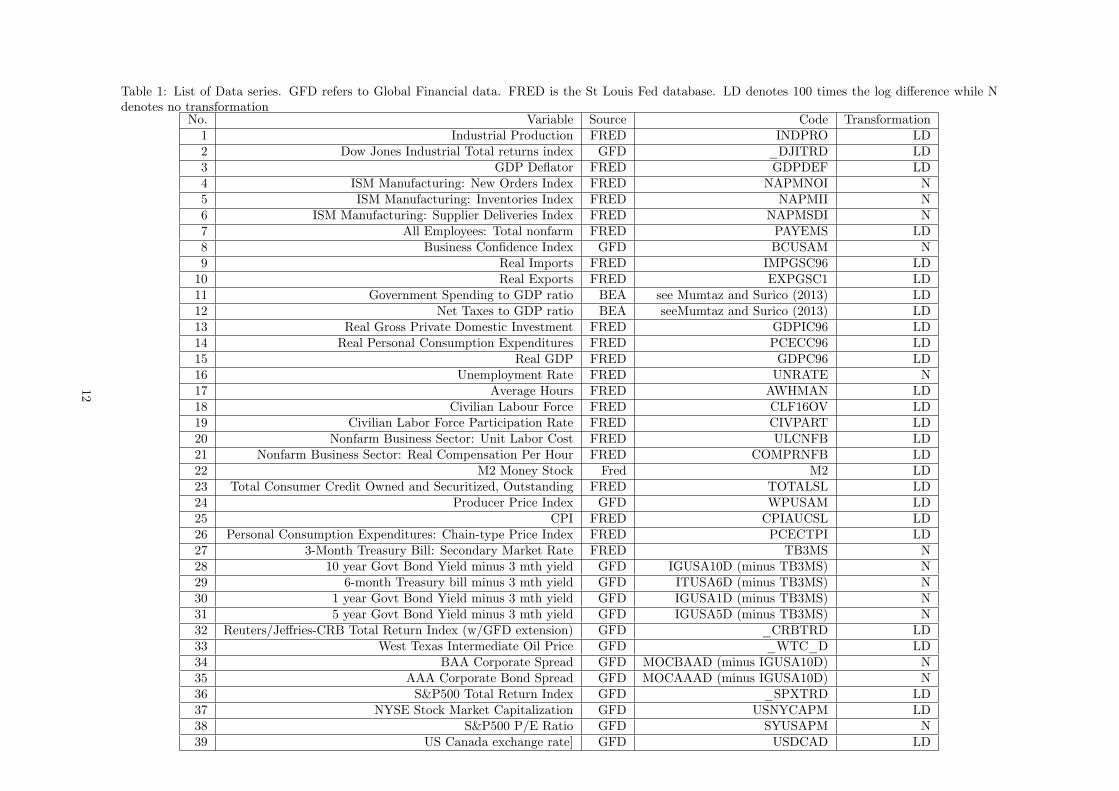
Table 1: List of Data series. GFD refers to Global Financial data. FRED is the St Louis Fed database. LD denotes 100 times the log difference while Ndenotes no transformation

No. Variable Source Code Transformation1 Industrial Production FRED INDPRO LD2 Dow Jones Industrial Total returns index GFD _DJITRD LD3 GDP Deflator FRED GDPDEF LD4 ISM Manufacturing: New Orders Index FRED NAPMNOI N5 ISM Manufacturing: Inventories Index FRED NAPMII N6 ISM Manufacturing: Supplier Deliveries Index FRED NAPMSDI N7 All Employees: Total nonfarm FRED PAYEMS LD8 Business Confidence Index GFD BCUSAM N9 Real Imports FRED IMPGSC96 LD10 Real Exports FRED EXPGSC1 LD11 Government Spending to GDP ratio BEA see Mumtaz and Surico (2013) LD12 Net Taxes to GDP ratio BEA seeMumtaz and Surico (2013) LD13 Real Gross Private Domestic Investment FRED GDPIC96 LD14 Real Personal Consumption Expenditures FRED PCECC96 LD15 Real GDP FRED GDPC96 LD16 Unemployment Rate FRED UNRATE N17 Average Hours FRED AWHMAN LD18 Civilian Labour Force FRED CLF16OV LD19 Civilian Labor Force Participation Rate FRED CIVPART LD20 Nonfarm Business Sector: Unit Labor Cost FRED ULCNFB LD21 Nonfarm Business Sector: Real Compensation Per Hour FRED COMPRNFB LD22 M2 Money Stock Fred M2 LD23 Total Consumer Credit Owned and Securitized, Outstanding FRED TOTALSL LD24 Producer Price Index GFD WPUSAM LD25 CPI FRED CPIAUCSL LD26 Personal Consumption Expenditures: Chain-type Price Index FRED PCECTPI LD27 3-Month Treasury Bill: Secondary Market Rate FRED TB3MS N28 10 year Govt Bond Yield minus 3 mth yield GFD IGUSA10D (minus TB3MS) N29 6-month Treasury bill minus 3 mth yield GFD ITUSA6D (minus TB3MS) N30 1 year Govt Bond Yield minus 3 mth yield GFD IGUSA1D (minus TB3MS) N31 5 year Govt Bond Yield minus 3 mth yield GFD IGUSA5D (minus TB3MS) N32 Reuters/Jeffries-CRB Total Return Index (w/GFD extension) GFD _CRBTRD LD33 West Texas Intermediate Oil Price GFD _WTC_D LD34 BAA Corporate Spread GFD MOCBAAD (minus IGUSA10D) N35 AAA Corporate Bond Spread GFD MOCAAAD (minus IGUSA10D) N36 S&P500 Total Return Index GFD _SPXTRD LD37 NYSE Stock Market Capitalization GFD USNYCAPM LD38 S&P500 P/E Ratio GFD SYUSAPM N39 US Canada exchange rate] GFD USDCAD LD

12

1.8 Recursive means

Figure 4 presents the mean of the Gibbs draws for key model parameters calculated every 100 draws. These arefairly stable which provides evidence of convergence of the Gibbs algorithm.

2 Details on the DSGE model

2.1 Calibration

The benchmark calibration is listed in table 3. The parametrization of the non-financial block of the of the model isbased on Fernandez-Villaverde and Rubio-Ramirez (2008), while the calibration of the financial block of the modelrelies on Christiano et al. (2014). In both studies full information Bayesian estimation techniques have been usedto decide about the structural parameter and this is what drives our selection. However, for the purposes of thesimulation experiments discussed in the main text we have changed the values of γπ, π, θp, χ, ΛA, η and ε relative tothe numbers reported by Fernandez-Villaverde and Rubio-Ramirez (2008) (Table 2.1). To be precise, the discountfactor is set equal to 0.999 and combined with the inflation target π = 1.010, the growth rates of the investmentspecific technological change Λμ = 1.010 and of the neutral technology ΛA = 1.0013, implies that the steady-statevalue of the annual real rate is 6.40%. The degree of habit persistence is 0.88, this value is higher than the estimatesreported by Smets and Wouters (2007) and Justiniano et al. (2010), however, due to log consumption preferencesa high degree of habit persistence is needed so demand does not display excess sensitivity to the real interest rate(via the Euler consumption equation). Similar to Smets and Wouters (2007) the inverse Frisch elasticity of laboursupply is equal to 1.36 and the investment adjustment is equal to 7.68 suggesting very little response of investmentto changes in Tobin’s q. The Calvo parameters imply that prices and wages are reset every 2.22 and 3.33 quartersrespectively, while households rely on indexation (χw = 0.80) more heavily than firms (χ = 0.40). The elasticitiesof substitution ε for firms and η for households imply an average markup of around 5% and 30%, respectively. TheTaylor rule parameters are γπ = 1.010, γy = 0.190 and γR = 0.79. The steady-state probability of defaults is 2.24%and slightly smaller than the value 3% used in the literature (see Bernanke et al. (1999)). The value of entrepreneurauditing cost is 0.21 and the fraction of survival entrepreneurs is 0.985, again these values are higher than thoseused in the literature (3% and 0.976 Bernanke et al. (1999)).

2.2 Solution

The model is solved using third-order perturbation methods (see Judd (1998)) as for any order lower than three,uncertainty shocks (our main objects of interest) do not enter into the decision rule as independent components.One difficulty of using these higher-order solution techniques is that paths simulated by the approximated policyfunction often explode. This is because regular perturbation approximations are polynomials that have multiplesteady states and could yield unbounded solutions (Kim et al., 2008). This means that the approximation is validonly locally and along the simulation path we may enter into a region where its validity is not preserved anymore.To avoid this problem Kim et al. (2008) suggest to ‘prune’ all those terms that have an order that is higher than

the approximation order, while Andreasen et al. (2013) show how this logic can be applied to any order. Althoughthere are studies that question the legitimacy of this approach (see Haan and Wind (2010)), it has by now beenwidely accepted as the only reliable way to get the solution of nth order approximated DSGE model (where n > 1).

Finally, we follow Fernández-Villaverde et al. (2011) and generate the responses of model variables to stochasticvolatility shocks using generalised impulse responses developed by Koop et al. (1996).

2.3 IRFs

The exact simulation steps to produce the impulse responses reported here are as follows:

1. We draw 5 × 1040 structural shocks ωj,t from the standard normal distribution (where j = 1, .., 5 and t =1, .., 1040)

2. We simulate the model using the shocks from step 1, we denote the simulated data by yt

3. We simulate the model using again the structural shocks ωj,t from step 1 but now we increase the value of thestructural shock of interest in period 1001 by an amount necessary to rise uncertainty by 1 times the standarddevition of the uncertainty shock, namely

ωj,1001 = ωj,1001 + x (9)

13

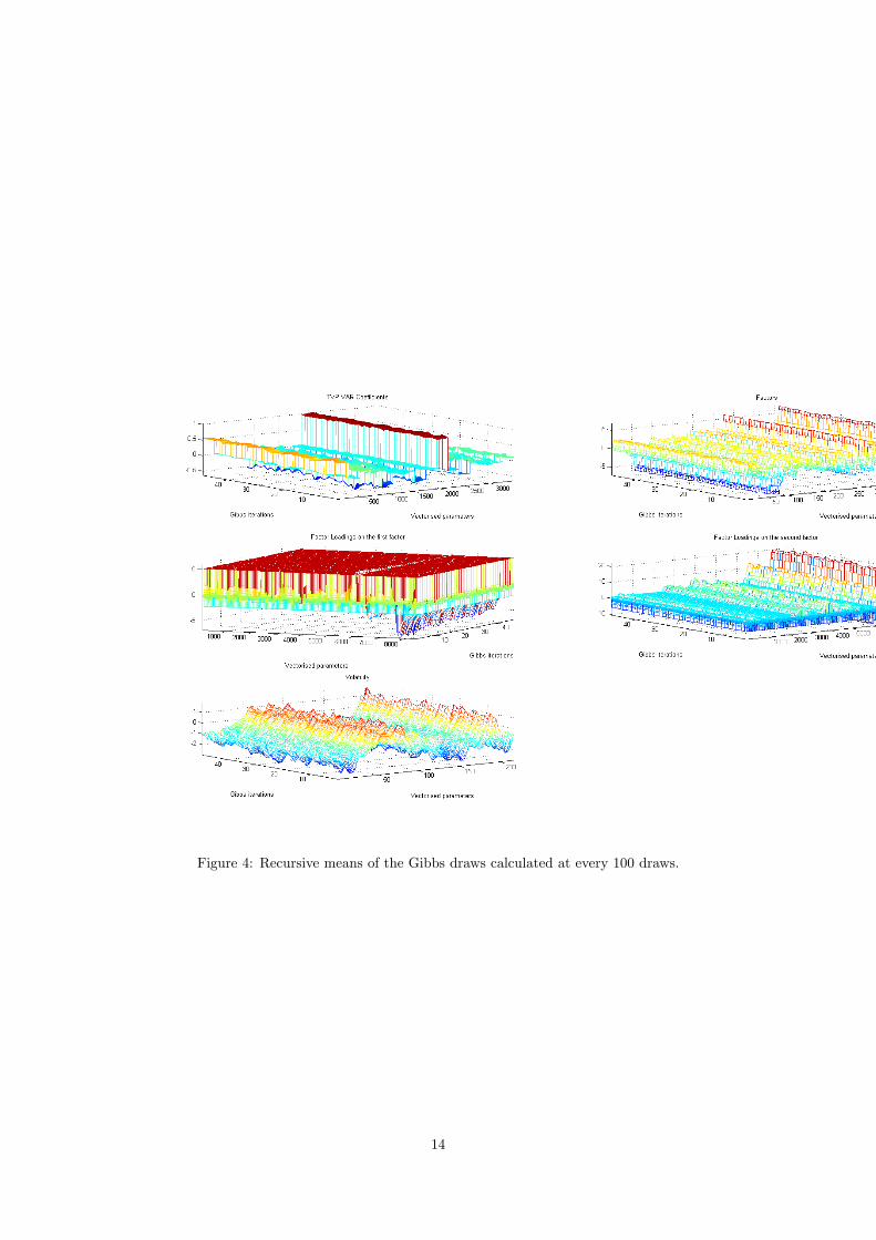
Figure 4: Recursive means of the Gibbs draws calculated at every 100 draws.

14

We denote the data obtained from this simulation by yt

4. Steps 1 to 3 are repeated 1000 times

5. The IRF is calculated as follows

IRF =1

1000

1000∑i=1

(yit − yit

)(10)

All calculations have been produced using Dynare 4.4.2 and Matlab 2012b.

15

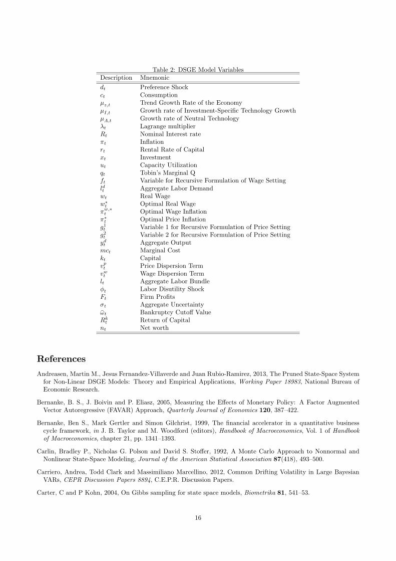
Table 2: DSGE Model VariablesDescription Mnemonic

dt Preference Shockct Consumptionμz,t Trend Growth Rate of the EconomyμI,t Growth rate of Investment-Specific Technology GrowthμA,t Growth rate of Neutral Technologyλt Lagrange multiplierRt Nominal Interest rateπt Inflationrt Rental Rate of Capitalxt Investmentut Capacity Utilizationqt Tobin’s Marginal Qft Variable for Recursive Formulation of Wage Settingldt Aggregate Labor Demandwt Real Wagew∗t Optimal Real Wageπw,∗t Optimal Wage Inflationπ∗t Optimal Price Inflationg1t Variable 1 for Recursive Formulation of Price Settingg2t Variable 2 for Recursive Formulation of Price Settingydt Aggregate Outputmct Marginal Costkt Capitalvpt Price Dispersion Termvwt Wage Dispersion Termlt Aggregate Labor Bundleφt Labor Disutility ShockFt Firm Profitsσt Aggregate Uncertaintyωt Bankruptcy Cutoff ValueRkt Return of Capitalnt Net worth

References

Andreasen, Martin M., Jesus Fernandez-Villaverde and Juan Rubio-Ramirez, 2013, The Pruned State-Space Systemfor Non-Linear DSGE Models: Theory and Empirical Applications, Working Paper 18983, National Bureau ofEconomic Research.

Bernanke, B. S., J. Boivin and P. Eliasz, 2005, Measuring the Effects of Monetary Policy: A Factor AugmentedVector Autoregressive (FAVAR) Approach, Quarterly Journal of Economics 120, 387—422.

Bernanke, Ben S., Mark Gertler and Simon Gilchrist, 1999, The financial accelerator in a quantitative businesscycle framework, in J. B. Taylor and M. Woodford (editors), Handbook of Macroeconomics, Vol. 1 of Handbookof Macroeconomics, chapter 21, pp. 1341—1393.

Carlin, Bradley P., Nicholas G. Polson and David S. Stoffer, 1992, A Monte Carlo Approach to Nonnormal andNonlinear State-Space Modeling, Journal of the American Statistical Association 87(418), 493—500.

Carriero, Andrea, Todd Clark and Massimiliano Marcellino, 2012, Common Drifting Volatility in Large BayesianVARs, CEPR Discussion Papers 8894, C.E.P.R. Discussion Papers.

Carter, C and P Kohn, 2004, On Gibbs sampling for state space models, Biometrika 81, 541—53.

16

Christiano, Lawrence, Roberto Motto and Massimo Rostagno, 2014, Risk Shocks, American Economic Review104(1), 27—65.

Cogley, T. and T. J. Sargent, 2005, Drifts and Volatilities: monetary policies and outcomes in the Post WWII U.S.,Review of Economic Dynamics 8, 262—302.

Fernandez-Villaverde, Jesus and Juan F. Rubio-Ramirez, 2008, How Structural Are Structural Parameters?, NBERMacroeconomics Annual 2007, Volume 22, NBER Chapters, National Bureau of Economic Research, Inc, pp. 83—137.

Fernández-Villaverde, Jesús, Pablo A. Guerrón-Quintana, Keith Kuester and Juan Rubio-Ramírez, 2011, FiscalVolatility Shocks and Economic Activity, NBER Working Papers 17317, National Bureau of Economic Research,Inc.

Gamble, James A. and James P. LeSage, 1993, A Monte Carlo Comparison of Time Varying Parameter andMultiprocess Mixture Models in the Presence of Structural Shifts and Outliers, The Review of Economics andStatistics 75(3), pp. 515—519.

Haan, Wouter Den and Joris De Wind, 2010, How well-behaved are higher-order perturbation solutions?, Dnbworking papers.

Jacquier, E, N Polson and P Rossi, 1994, Bayesian analysis of stochastic volatility models, Journal of Business andEconomic Statistics 12, 371—418.

Judd, Kenneth, 1998, Numerical Methods in Economics, MIT Press, Cambridge.

Justiniano, Alejandro, Giorgio Primiceri and Andrea Tambalotti, 2010, Investment shocks and business cycles,Journal of Monetary Economics 57(2), 132—45.

Kim, Jinill, Sunghyun Kim, Ernst Schaumburg and Christopher Sims, 2008, Calculating and using second-orderaccurate solutions of discrete time dynamic equilibrium models, Journal of Economic Dynamics and Control32(11), 3397 — 414.

Koop, Gary, M. Hashem Pesaran and Simon M. Potter, 1996, Impulse response analysis in nonlinear multivariatemodels, Journal of Econometrics 74(1), 119—147.

Mumtaz, Haroon and Paolo Surico, 2013, Policy Uncertainty and Aggregate Fluctuations, Working Papers 708,Queen Mary, University of London, School of Economics and Finance.

Primiceri, G, 2005, Time varying structural vector autoregressions and monetary policy, The Review of EconomicStudies 72(3), 821—52.

Smets, Frank and Rafael Wouters, 2007, Shocks and Frictions in US Business Cycles: a Bayesian DSGE Approach,American Economic Review 97, 586—606.

17

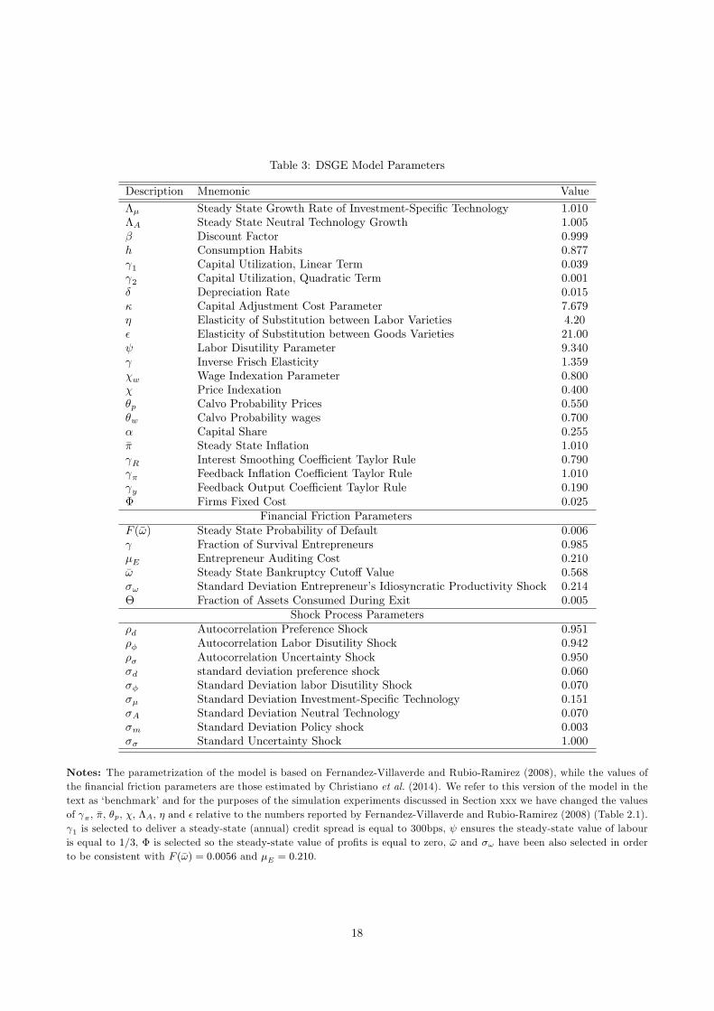
Table 3: DSGE Model Parameters

Description Mnemonic Value

Λμ Steady State Growth Rate of Investment-Specific Technology 1.010ΛA Steady State Neutral Technology Growth 1.005β Discount Factor 0.999h Consumption Habits 0.877γ1 Capital Utilization, Linear Term 0.039γ2 Capital Utilization, Quadratic Term 0.001δ Depreciation Rate 0.015κ Capital Adjustment Cost Parameter 7.679η Elasticity of Substitution between Labor Varieties 4.20ε Elasticity of Substitution between Goods Varieties 21.00ψ Labor Disutility Parameter 9.340γ Inverse Frisch Elasticity 1.359χw Wage Indexation Parameter 0.800χ Price Indexation 0.400θp Calvo Probability Prices 0.550θw Calvo Probability wages 0.700α Capital Share 0.255π Steady State Inflation 1.010γR Interest Smoothing Coefficient Taylor Rule 0.790γπ Feedback Inflation Coefficient Taylor Rule 1.010γy Feedback Output Coefficient Taylor Rule 0.190Φ Firms Fixed Cost 0.025

Financial Friction ParametersF (ω) Steady State Probability of Default 0.006γ Fraction of Survival Entrepreneurs 0.985μE Entrepreneur Auditing Cost 0.210ω Steady State Bankruptcy Cutoff Value 0.568σω Standard Deviation Entrepreneur’s Idiosyncratic Productivity Shock 0.214Θ Fraction of Assets Consumed During Exit 0.005

Shock Process Parametersρd Autocorrelation Preference Shock 0.951ρφ Autocorrelation Labor Disutility Shock 0.942ρσ Autocorrelation Uncertainty Shock 0.950σd standard deviation preference shock 0.060σφ Standard Deviation labor Disutility Shock 0.070σμ Standard Deviation Investment-Specific Technology 0.151σA Standard Deviation Neutral Technology 0.070σm Standard Deviation Policy shock 0.003σσ Standard Uncertainty Shock 1.000

Notes: The parametrization of the model is based on Fernandez-Villaverde and Rubio-Ramirez (2008), while the values ofthe financial friction parameters are those estimated by Christiano et al. (2014). We refer to this version of the model in thetext as ‘benchmark’ and for the purposes of the simulation experiments discussed in Section xxx we have changed the valuesof γπ, π, θp, χ, ΛA, η and ε relative to the numbers reported by Fernandez-Villaverde and Rubio-Ramirez (2008) (Table 2.1).γ1 is selected to deliver a steady-state (annual) credit spread is equal to 300bps, ψ ensures the steady-state value of labouris equal to 1/3, Φ is selected so the steady-state value of profits is equal to zero, ω and σω have been also selected in orderto be consistent with F (ω) = 0.0056 and μE = 0.210.

18

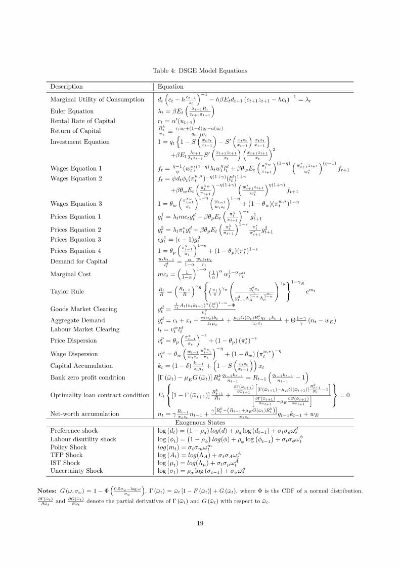
Table 4: DSGE Model Equations

Description Equation

Marginal Utility of Consumption dt

(ct − h ct−1zt

)−1− hβEtdt+1 (ct+1zt+1 − hct)−1 = λt

Euler Equation λt = βEt

(λt+1Rt

zt+1πt+1

)Rental Rate of Capital rt = α

′(ut+1)

Return of Capital Rkt

πt≡ rtut+(1−δ)qt−a(ut)

qt−1μt

Investment Equation 1 = qt

{1− S

(xtztxt−1

)− S′

(xtztxt−1

)xtztxt−1

}+βEt

λt+1λtzt+1

S′(xt+1zt+1

xt

)(xt+1zt+1

xt

)2Wages Equation 1 ft =

η−1η (w∗t )

(1−η)λtwηt ldt + βθwEt

(πχwt

πt+1

)(1−η) (w∗t+1zt+1w∗t

)(η−1)ft+1

Wages Equation 2 ft = ψdtφt(πw,∗t )−η(1+γ)(ldt )

1+γ

+βθwEt

(πχwt

πt+1

)−η(1+γ) (w∗t+1zt+1w∗t

)η(1+γ)ft+1

Wages Equation 3 1 = θw

(πχwt−1πt

)1−η (wt−1wtzt

)1−η+ (1− θw)(πw,∗t )1−η

Prices Equation 1 g1t = λtmctydt + βθpEt

(πχtπt+1

)−εg1t+1

Prices Equation 2 g2t = λtπ∗t ydt + βθpEt

(πχtπt+1

)1−επ∗tπ∗t+1

g2t+1Prices Equation 3 εg1t = (ε− 1)g2tPrices Equation 4 1 = θp

(πχt−1πt

)1−ε+ (1− θp)(π∗t )1−ε

Demand for Capital utkt−1ldt

= α1−α

wtztμtrt

Marginal Cost mct =(

11−α

)1−α (1α

)αw1−αt rαt

Taylor Rule Rt

R =(Rt−1R

)γR {(πtπ

)γπ ( ydt zt

ydt−1Λ1

1−αA Λ

α1−αμ

)γy}1−γRemt

Goods Market Clearing ydt =1ztAt(utkt−1)α(ldt )

1−α−Φvpt

Aggregate Demand ydt = ct + xt +α(ut)kt−1ztμt

+μEG(ωt)R

kt qt−1kt−1

ztπt+Θ 1−γ

γ (nt − wE)Labour Market Clearing lt = v

wt ldt

Price Dispersion vpt = θp

(πχt−1πt

)−ε+ (1− θp) (π∗t )−ε

Wage Dispersion vwt = θw

(wt−1wtzt

πχwt−1πt

)−η+ (1− θw)

(πw,∗t

)−ηCapital Accumulation kt = (1− δ) kt−1ztμt

+(1− S

(xtztxt−1

))xt

Bank zero profit condition [Γ (ωt)− μEG (ωt)]Rkt qt−1kt−1nt−1= Rt−1

(qt−1kt−1nt−1

− 1)

Optimality loan contract condition Et

⎧⎨⎩[1− Γ (ωt+1)] R

kt+1

Rt+

∂Γ(ωt+1)∂ωt+1

[[Γ(ωt+1)−μEG(ωt+1)]

Rkt+1Rt

−1]

[∂Γ(ωt+1)∂ωt+1

−μE∂G(ωt+1)∂ωt+1

]⎫⎬⎭ = 0

Net-worth accumulation nt = γRt−1πtzt

nt−1 +γ[Rk

t−(Rt−1+μEG(ωt)Rkt )]

πtztqt−1kt−1 + wE

Exogenous StatesPreference shock log (dt) = (1− ρd) log(d) + ρd log (dt−1) + σtσdωdtLabour disutility shock log (φt) =

(1− ρφ

)log(φ) + ρφ log

(φt−1

)+ σtσφω

φt

Policy Shock log(mt) = σtσmωmt

TFP Shock log (At) = log(ΛA) + σtσAωAt

IST Shock log (μt) = log(Λμ) + σtσμωAt

Uncertainty Shock log (σt) = ρσ log (σt−1) + σσωσt

Notes: G (ω, σω) = 1 − Φ(0.5σω−logω

σω

), Γ (ωt) = ωt [1− F (ωt)] + G (ωt), where Φ is the CDF of a normal distribution.

∂Γ(ωt)∂ωt

and ∂G(ωt)∂ωt

denote the partial derivatives of Γ (ωt) and G (ωt) with respect to ωt.

19

This working paper has been produced bythe School of Economics and Finance atQueen Mary University of London

Copyright © 2014 Haroon Mumtaz and Konstantinos Theodoridis

School of Economics and FinanceQueen Mary University of LondonMile End RoadLondon E1 4NSTel: +44 (0)20 7882 7356Fax: +44 (0)20 8983 3580Web: www.econ.qmul.ac.uk/research/workingpapers/

All rights reserved