Working Paper Series WP 2017-13

School of Economic Sciences

Adjusting Self-Assessed Health for Potential Bias Using a Random-Effects Generalized Ordered

Probit model

Qingqing Yang and Robert Rosenman

September 2017

1

Adjusting Self-Assessed Health for Potential Bias

Using a Random-Effects Generalized Ordered Probit model

Qingqing Yang

School of Economic Sciences

Washington State University

Pullman, WA 99163

qingqing.yang@wsu.edu

Robert Rosenman

School of Economic Sciences

Washington State University

Pullman, WA 99163

yamaka@wsu.edu

Copyright 2016 by [Qingqing Yang and Robert Rosenman]. All rights reserved. Readers may make

verbatim copies of this document for non-commercial purposes by any means, provided that this

copyright notice appears on all such copies.

The authors are Ph.D. Graduate Research Assistant and Professor, respectively, in the School of Economic Sciences,

Washington State University. This research uses data from China Health and Nutrition Survey (CHNS). We thank

the National Institute of Nutrition and Food Safety, China Center for Disease Control and Prevention, Carolina

Population Center, the University of North Carolina at Chapel Hill, the NIH (R01-HD30880, DK056350, and R01-

HD38700) and the Fogarty International Center, NIH for financial support for the CHNS data collection and

analysis files from 1989 to 2006 and both parties plus the China-Japan Friendship Hospital, Ministry of Health for

support for CHNS 2009 and future surveys.

2

Abstract

In this paper we assess how socioeconomic conditions affect self-assessed health and objective

measure of health. Using a random-effects generalized ordered probit model with data from

China Health and Nutrition Survey, we test for heterogeneity by socioeconomic status. The

results show that individuals with high income relative to a comparison group are less likely to

self-assess poor health; they are more likely to report good health; but they are not more likely to

report extremely good health. These socioeconomic variables do not significantly affect an

objective measure of health. Although SAH captures many aspects of health elements, it might

be biased on some socioeconomic features.

Keywords: SAH, Reporting Heterogeneity, relative income

JEL classification: I12, I14, C25

3

1. Introduction

Self-assessed health (SAH) is a commonly used measure of individual health in a wide range of

policy studies. It is often used to analyze how health responds to lifestyle and policy, as well as

in distributional studies (Contoyannis and Jones 2004, Balia and Jones 2008, Costa-Font, et al.

2013). But it is often asked how well SAH adequately measures true health.

There is some evidence that SAH may be malleable depending on the survey method. Crossley

and Kennedy (2002), using data from the Australian National Health Survey show that 28% of

respondents in a random sub-sample which was surveyed twice changed their SAH level after

giving answers to additional health related questions. Clarke and Ryan (2006) found a similar

variation when SAH was again asked twice of respondents (the first in a personal interview and

second in a self-completion survey). Greene at el. (2014) note an inflation of SAH. They found

that “the overwhelming majority of responses fall in either the middle category or the one

immediately to (its) ‘right’” and such responses are more favorable than should be expected

given more objective medical indicators.

Because SAH is a subjective reporting index, there is also an immediate concern about

heterogeneity in reporting. Shmueli (2003) shows extensive reporting heterogeneity in SAH that

depends on a large number of socioeconomic factors, including income. Vaillant and Wolfe

(2012) find the difference between SAH and objective measures is more pronounced between

individuals than it is within individuals over time. One possible explanation for socioeconomic

related heterogeneity is a difference in reference groups or points, depending on their

demographic and social-economic characteristics (Kerkhofs and Lindeboom, 1995; Lindeboom

and Van Doorslaer, 2004). Lindeboom and Van Doorslaer (2004) proposes a test for differential

4

reporting in ordered response models which enables to distinguish between cut-point shift and

index shift using Canadian National Population Health Survey data. They find clear evidence of

index shifting and cut-point shifting for age and gender, but not for income, education or

language.

The hypothesis underlying the present paper is that individuals’ assessment of their own health

may depend on one’s relative condition in one’s subgroup. In research about happiness, Easterlin

(1974, 1995) argues that within a country at a given time those with higher incomes are, on

average, happier. However, raising the incomes of all does not increase the happiness of all

because it is relative income not absolute income which affects happiness. We believe that SAH

may have a similar relationship, where the comparison group for an individual might be defined

by a localized reference group. To the extent socioeconomic variables like ethnicity and income

determine a localized reference group, they would therefore affect SAH, an idea propagated in

Wilkinson (1997). Raising the income of all may increase the health of all, but may not increase

the SAH of all, especially for those with high income level.

In the research cited above, most papers use Ordered Probit or Logit models, assuming that the

coefficients of independent variables do not vary between categories of the dependent variable.

This assumption conceals possible heterogeneous effects of some independent variables. In

addition, none use relative socioeconomic status in the regression. To fill these gaps in literature,

we use a Random-Effects Generalized Ordered Probit Model (Pfarr et al., 2011), to identify the

correlation with SAH and how the cut-points in assessing health vary with socioeconomic factors.

Most specifically, we are interested in how relative income influences self-assessed health status.

We also test for bias in SAH by using an objective health measure as the dependent variable in

an otherwise identical model. Most socioeconomic variables affect people’s SAH, but not affect

5

the objective health measure. Hence, this provides evidence that these variables cause a bias in

SAH.

The rest of the paper is organized as follows. Section 2 introduces the framework of the random

effect generalized ordered probit model; Section 3 introduces the data and variables we use in the

analysis. The results are discussed in part 4, and part 5 offers conclusions.

2. The Empirical Framework

The World Health Organization (WHO) defines health as “a state of complete physical, mental

and social well-being and not merely the absence of disease or infirmity” (WHO,

www.who.int/about/definition/en/print.html). Objective measures of health usually focus on

disease or infirmity (the part of this definition that WHO categorically rejects as a whole

measure of health) building functional indices founded on diagnostic, prognostic, and evaluative

criterion (McDowell, 2006) or the incidence or absence of specific ailments. SAH, on the other

hand, is more abstractly defined, with individuals asked to assign themselves to discrete

categories that range from poor to excellent, often without much guidance. Underlying both

objective measures of health and SAH is true health. Because one component of true health is

the presence or absence of disease, it is likely that when people assess their health some

objective measures of health go into that assessment. The random effects generalized ordered

probit model that follows takes such behavior into account (Pfarr et al., 2010, 2011).

True health *

itH , individual i’s health status in time t, is an unobserved latent variable governed

by the equation

6

* ' , ~ (0,1)it i it it itH X N

Where '

itX is a vector of independent variables which help determine true health. In the random

effects panel data model 𝛼𝑖 represents an individual effect with a zero mean and variance 2 , so

2 2/ (1 ) is the share of total variability in 𝐻𝑖𝑡∗, attributable to the individual effect. The

vector 𝛽 are parameters and 𝜀𝑖𝑡 is a random term independent of individual characteristics.

Included in the vector of independent variables are individuals’ demographic and socio-

economic features, lifestyle, genetic disposition, current ailments and diseases, and luck. Let

S

itH be self-assessed health (SAH), usually obtained by survey. People are asked a question like

“What do you think about your health status”, choosing from a numerical scale to represent poor,

fair, good and excellent health. In our data, SAH is given by a four point scale. We assume

underlying the regression is the following decision;

𝐻𝑖𝑡𝑆 = 1 ↔ 𝐻𝑖𝑡

∗ ≤ 𝜇𝑖1

𝐻𝑖𝑡𝑆 = 𝑗 ↔ 𝜇𝑖𝑗−1 < 𝐻𝑖𝑡

∗ ≤ 𝜇𝑖𝑗 , 𝑗 = 2, 3 (1)

𝐻𝑖𝑡𝑆 = 4 ↔ 𝐻𝑖

∗ > 𝜇𝑖3

𝜇𝑖𝑗 = 𝜇𝑗 + 𝑧𝑖′𝛾𝑗 (2)

which is a form of censoring. The 𝜇𝑖𝑗 ’s are unknown individual specific parameters to be

estimated with 𝛽.

With four categories we have three thresholds; 𝜇𝑖1 = 0, 𝜇𝑖2 = 𝜇2 + 𝑧𝑖′𝛾2, 𝜇𝑖3 = 𝜇3 + 𝑧𝑖

′𝛾3

where 𝛾2 and 𝛾3 are parameters to be estimated and 𝑧𝑖 is a subset of 𝑋𝑖𝑡. The model is equivalent

to three binary logistic regressions where categories of the dependent variables are combined; to

find 𝜇𝑖1 category 𝐻𝑖𝑡𝑆 = 1 is contrasted against categories 𝐻𝑖𝑡

𝑆 = 2,3,4 ; for 𝜇𝑖2 categories

7

𝐻𝑖𝑡𝑆 = 1, 2 are contrasted with 𝐻𝑖𝑡

𝑆 = 3, 4 ; and to find 𝜇𝑖3 categories 𝐻𝑖𝑡𝑆 = 1, 2, 3 are

contrasted against category 𝐻𝑖𝑡𝑆 = 4 (Williams 2006). If 𝛾2 and 𝛾3 are nonzero, the thresholds

are conditional on 𝑧𝑖, unlike the normal probit model where the thresholds are the same for all

individuals.1 Hence a generalized ordered probit model accounts for individual heterogeneity

through the thresholds.2 Imposing our functional forms for the thresholds we have

𝐻𝑖𝑡𝑆 = 1 𝑖𝑓 𝐻𝑖𝑡

∗ ≤ 0

𝐻𝑖𝑡𝑆 = 2 𝑖𝑓 0 ≤ 𝐻𝑖𝑡

∗ ≤ 𝜇2 + 𝑧𝑖′𝛾2

𝐻𝑖𝑡𝑆 = 3 𝑖𝑓 𝜇2 + 𝑧𝑖

′𝛾2 ≤ 𝐻𝑖𝑡∗ ≤ 𝜇3 + 𝑧𝑖

′𝛾3

𝐻𝑖𝑡𝑆 = 4 𝑖𝑓 𝐻𝑖𝑡

∗ ≥ 𝜇3 + 𝑧𝑖′𝛾3

which gives the following probabilities

𝑃1 = 𝑃𝑟𝑜𝑏(𝐻𝑖𝑡𝑆 = 1 |𝑋𝑖, 𝑍𝑖𝑡) = F(−𝛼𝑖 − 𝑋𝑖𝑡

′ 𝛽)

𝑃2 = 𝑃𝑟𝑜𝑏(𝐻𝑖𝑡𝑆 = 2 |𝑋𝑖𝑡

′ , 𝑍𝑖𝑡) = F(𝜇2 + 𝑧𝑖𝑡′ 𝛾2 − (𝛼𝑖 + 𝑋𝑖𝑡

′ 𝛽)) − F(−𝛼𝑖 − 𝑋𝑖𝑡′ 𝛽)

𝑃3 = 𝑃𝑟𝑜𝑏(𝐻𝑖𝑡𝑆 = 3 |𝑋𝑖𝑡

′ , 𝑍𝑖𝑡) = F(𝜇3 + 𝑧𝑖𝑡′ 𝛾3 − (𝛼𝑖 + 𝑋𝑖𝑡

′ 𝛽)) − F(𝜇2 + 𝑧𝑖𝑡′ 𝛾2 − (𝛼𝑖 + 𝑋𝑖𝑡

′ 𝛽))

𝑃4 = 𝑃𝑟𝑜𝑏(𝐻𝑖𝑡𝑆 = 4 |𝑋𝑖𝑡

′ , 𝑍𝑖𝑡) = 1 − F(𝜇3 + 𝑧𝑖𝑡′ 𝛾3 − (𝛼𝑖 + 𝑋𝑖𝑡

′ 𝛽))

We use MLE and a corresponding log-likelihood function

2 2

3 3 2

1 2

3

4

2

3 3

F ( )

F (

ln ( ' ) ' ' ( ' )

' ' ' '

' '

) F ( )

1-F ( )

S Sit it

Sit

Sit

i it it it i it

H H

it it it it

H

it it

H

i

i i

i

L F X Z X F X

Z X Z X

Z X

1 The traditional ordered probit assumes the categories are “parallel” and differ only by the intercept. The generalized ordered probit does not impose this assumption, which is often violated in practice. 2 It is common to report the results from Generalized Ordered Probit as (in our case) three different sets of

estimates that include the thresholds in the estimates of and then separately report the values of the i. This is how we report our results in Tables 4A and 4B below.

8

3. Data

We use the data from China Health and Nutrition Survey (CHNS), which is an international

collaborative project between the Carolina Population Center at the University of North Carolina

at Chapel Hill and the National Institute of Nutrition and Food Safety at the Chinese Center for

Disease Control and Prevention. This survey was conducted in nine provinces in China for nine

waves from year 1989 to year 2011. Among the dataset, there are 4 years with reported

individual’s self-assessed health (1997, 2000, 2004 and 2006). Since some individuals were not

surveyed every year, we use only those observations that have at least 3 years of data. After data

cleaning, the effective unbalanced panel includes 22055 observations. Among them, 4665

observations are in year 1997, 4983 observations are in year 2000, 6401 observations are in year

2004, and 5997 observations are in year 2006.

3.1 Variables: A production function for health

We follow the theoretic framework in Contoyannis and Jones (2004) to choose variables for

equations (1) and (2). Table 1 below shows the variables we include. For analytical purposes, we

divided the variables into groups representing health behaviors, objective health measures,

education, marital status, work status, physical and regional variables. Relative health was kept

as its own group.

Health behaviors include variables that measure sleep, smoking, habits on alcohol consumption

and exercise. Sleep is a dummy variable which takes a value 1 if an individual sleep 7 to 9 hours

and takes value 0 otherwise. For smoking, we divide people into three kinds, current smoker,

previous smoker and people who never smoked. Current smoker is the excluded category. We

use two variables to indicate alcohol consumption, “Alcohol_freq” and “Alcohol_occa”. People

9

who don’t drink alcohol at all are excluded. The “Exercise” variable takes value 1 if the person

participates at least one kind of exercise. The exercises in the survey included Kung Fu,

Gymnastics, dancing, acrobatics, Track and field (running, etc.), swimming, Soccer, basketball,

tennis, Badminton, volleyball and others. “Nobese” means the individual is not obese.

For the objective health measures, the survey asked respondents if a doctor had ever told them

they had one of five conditions, high blood pressure, diabetes, myocardial infarction, Apoplexy,

and Fracture. These chronic diseases were chosen because they affect people’s life quality in

many ways. Although they do not cause death in a short time, they are leading causes of death in

the long run.

(Insert Table 1. Independent variable)

Relative income is often considered a substitute for social class (Contoyannis and Jones 2004;

Wilkinson 1997). We hypothesize that people self-refer on specific socioeconomic features, for

example, comparing themselves to others of the same education level. Here we use relative

income in the same province3 and education level as two sources of self-reference. The relative

income of individual i , who lives in province j (or with education level j ), at year t is calculated

by the equation

_( )

itijt

jt

hhincrltv income

E hhinc

3 We tried to use relative income within a respondent’s town, but that provided insufficient variability as incomes do not vary much within towns. Moreover, we test, therefore, if people compare not just within their own community, but also to nearby communities. “Province” in China is like the concept of “State” in the US.

10

where ithhinc is the household income of individual i at time t , and ( ) jtE hhinc is the average

household income in province j (or with education level j ) at year t . When relative income

equals to 1 it means that income is at the average level. Individuals with income above average

have a relative income great than 1; those with an income below the average have a relative

income less than 1.

Most other grouped variables are self-explanatory except for “Urban_hukou”. Hukou is a special

concept in China for household registration. China has two kinds of Hukou that distinguish

people who live in city or urban area from people who live in rural area. Urban_hukou=1

indicates the respondent is registered in an urban area.

3.2 Descriptive analysis

Table 2A presents the mean values of the variables by the four SAH subgroups. The subgroup

reporting SAH=1 feel their health status is “poor”. SAH=2 means health level is “fair”; SAH=3

means health level is “good”; SAH=4 indicates health level “excellent”.

Relative income, both refer to the same province and same education level is highly related to

SAH status. Both “good” health and “excellent” health subgroups have above average incomes.

People who assess their health as poor have income significantly lower than the average.

However, the difference between the excellent and good health subgroups is less significant than

the difference between other SAH subgroups.

Among the behavior variables, sleep has an ambiguous trend among the four SAH subgroups,

while exercise has a clear increasing trend from unhealthy to healthy subgroups. From the

exercise and habits variables, we see people who feel healthy have a better habits and exercise

11

more. The poor-health subgroup has a higher proportion of non-smokers and former smokers.

People in the healthier subgroups have a lower rate of obesity.

Objective healthy measures are highly consistent with people’s SAH. People in the healthy SAH

subgroups have lower morbidity rates of all the diseases we use. Especially for the excellent

health subgroup, few people are diagnosed of those severe and chronic diseases. Individual’s

average number of illness decreases from poor health group to excellent health group.

(Insert Table 2A. Means of the variables by SAH subgroups)

People with more education tend to report higher levels of health. For example, the proportion of

individuals with middle school, high school and college or university degree (or higher)

increases as we move from unhealthy to healthy. However, a higher proportion of divorce and

separation are observed in fair and good subgroups. The proportion of single people is larger in

higher health levels.

A higher proportion of unemployed, house keeper, disable and retired people are observed in the

“poor” health subgroup. In addition, the rate of unemployed in subgroup SAH=1 is much higher

than that in other subgroups. The proportion of people doing agricultural labor work is higher in

“poor” and “fair” health subgroup.

Physical condition and living conditions also have a clear pattern. Those indicating they have

excellent health are more likely to be male, younger and taller. And those indicating poor health

and excellent health status are more likely to live in the urban areas.

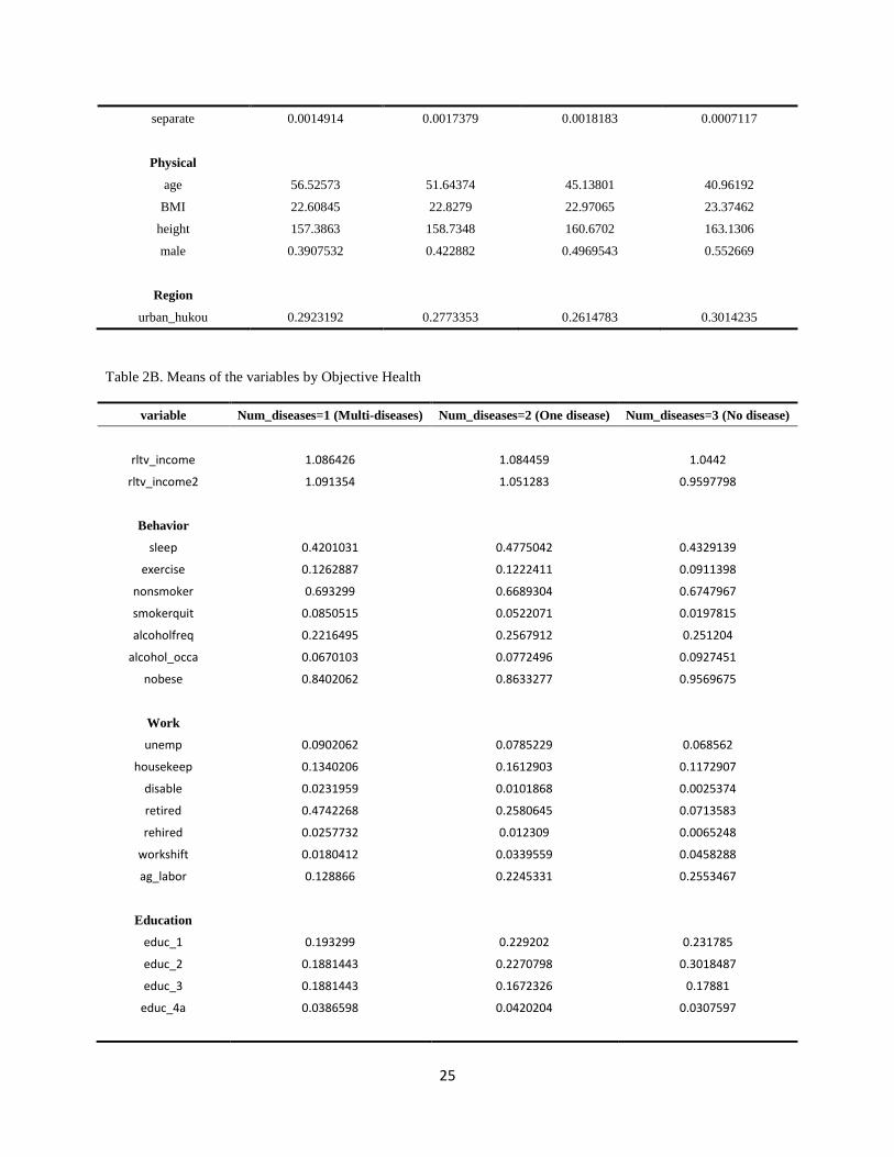
(Insert Table 2B. Means of the variables by Objective Health)

12

We then define an objective measure of health to compare with the SAH. As an objective

measure of health we used the number of severe or chronic diseases (denote as “Num_diseases”)

for which an individual has been diagnosed. The list of possible diseases includes high blood

pressure, diabetes, myocardial infarction, apoplexy, and fracture. To be consistent with the SAH

scale, “Num_diseases=1” represents for the most unhealthy group, which means the person has

more than one diseases; “Num_diseases=2” represents that the person has one of these diseases;

“Num_diseases=3” is the healthiest group, which means the person is diagnosed with none of

these diseases.

Table 2B shows the mean of variables by “Num_diseases”. Mean of the relative income doesn’t

change apparently. The healthiest group (Num_diseases=3, No disease) even has the relative

income slightly lower than the other two groups. A similar trend can be see regard to the

education variable. The proportion of people with lower education level (elementary school and

middle school degrees) increases when we move from the unhealthy group to healthy group,

while the proportion of observations with higher education level (high school and college or

above) decreases.

13

Figure 1. Relative household income distribution by SAH

(Without outliers greater than 1.5 times the 75th percentile)

Figure 1 shows the relative household income distribution by SAH subgroups in different years.

The line in the box is the medium of the relative income of every subgroup, while the boxes

represent the portion between the 25th percentile and the 75th percentile. In 1997, the box for the

poor health subgroup is below the dashed line. It means most people who report poor health earn

incomes below average. We expected that wealthier people would be healthier, but the excellent

health subgroup has a lower relative income when compared to the good health subgroup. The

same situation is observed in year 2000, but in 2004 and 2006 the healthiest subgroup has the

largest proportion of observations with a high relative household income. Compared to the other

-10

12

34

-10

12

34

poor fair good excellent poor fair good excellent

poor fair good excellent poor fair good excellent

1997 2000

2004 2006

Re

lative

Ho

use

ho

ld In

co

me

Data Source: CHNS

Relative income distribution by SAH Group (Without Outliers)

14

categories of SAH, the boxes for the poor health subgroup are comparatively narrow, indicating

the variation of relative income in this subgroup is less than in the other subgroups.

Figure 1. Relative household income distribution by SAH

(with outliers greater than 1.5 times the 75th percentile)

Figure 2 includes Outsider comparing the distribution of relative income by SAH group. The

fair and good health subgroups show a large spread of relative income, with high relative income

cluster in these two subgroups. The good health subgroup shows the largest spread.

Table 3 shows the correlation between the number of diagnosed illness and self-assessed health

disaggregated by relative income. People diagnosed with more kinds of diseases are less likely

to report good health, although the magnitude of the correlation is small. We note that the

correlation becomes strong when relative income increases.

05

10

15

05

10

15

poor fair good excellent poor fair good excellent

poor fair good excellent poor fair good excellent

1997 2000

2004 2006

Re

lative

Ho

use

ho

ld In

co

me

Data Source: CHNS

Relative income distribution by SAH Group (With Outliers)

15

(Insert Table 3. Correlation between number of illness and SAH)

4. Results

4.1 SAH as measure of health

Table 4A shows the results from two different regression models, a random effects ordered

probit and a random effects generalized ordered probit. SAH is used as a measure of health. As

we can see from table 4A, relative income, sleep, education degree of middle and high school,

single, widow, unemployment, disable, Urban_Hukou, male, height, diagnosed of hypertension

and apoplexy have different coefficients in the three parts of the generalized ordered probit

model, i.e., these variables violate the parallel line assumption. Table 4B show the coefficient 𝛾2

and 𝛾3 of these variables derived from the estimates in Table 4A.

(Insert Tables 4A and 4B. Random effect ordered probit and generalized ordered probit models)

We first pay attention to the variables that satisfy the parallel line assumption. The two smoking

behavior variables have opposite effect; people who quit smoking are more likely to report poor

health, while people who never smoke do not have a significant difference from current

smokers.4 The two alcohol behavior variables also have opposite sign coefficients, although only

frequent use is significant at conventional levels. Frequent alcohol users report good health status.

People usually doing exercise report better health than people who do not. Generally speaking,

people with more education report they are healthier. Divorced and separated people tend to

report poorer health than the base group, people who are married. Among the variables about

4 Poor health may lead people to quit smoking, creating an potential endogeneity problem with this variable that needs further exploration.

16

working status, people unemployed, involved in housekeeping and disabled, people who shift

work are all have worse self-assessed health than people work normally.

Of primary interest are those variables that violate the parallel assumption, especially relative

income. The result suggests that those who have higher relative income tend to report better

health. The positive effect of a relative income is especially high among those who report

themselves to be poor health as opposed to fair, good, or excellent health. When translated to the

coefficient (table 4B) it indicates that relative income lowers the threshold that pushes an

individual to the next highest level of SAH, so those with higher relative income are more likely

to be in the next highest category of SAH, indicating that those with higher relative income are

more likely to say their health is better if their SAH is in the fair or good categories. Relative

income is not statistically significant in the excellent health category. In sum, these results

indicate that having high relative income lowers the probability that people will self-assess their

health as poor, but also does not increase the probability that they will assess their health as

excellent.

Educational attainment may be another way people self-reference. Those who have a high-

school degree are unlikely to say they are in poor health, but are also unlikely to say they are in

excellent health. The estimates on good sleeping behavior are interesting. Generally, sleeping

well has a positive effect for the individual to choose fair or good health against poor health level,

but they are also unlikely to choose excellent health level compare to good, fair and poor. Living

in an urban area increases the probability of feeling extremely healthy. Compared to females,

males are more conservative about assessing good health -- they concentrate in the two middle

categories. Tall people self-assess healthier, and the effect becomes stronger when health level

increases. All the disease variables make people feel unhealthy. We also report for both

17

models in Table 4A. In both models, about 22 percent of total variation in SAH can be attributed

to individual fixed effects. This translates to a variance of about 0.282 for i .

(Insert Table 5. Random effect generalized ordered probit model with variable relative BMI)

As indicated, SAH is affected by the person’s objective health. Table 5 shows the results adding

variable relative BMI to the model. Even though relative BMI is significant with a p-value<0.001,

the signs and significance of the other variables is consistent with the earlier results.

(Insert Table 6. Marginal effect of random effect generalized ordered probit model)

Table 6 provides the marginal effect of the random effect generalized ordered probit model.

When relative income increases by 1 unit, the probability of reporting poor health decreases by

about 1% while the probability of reporting good health increases by 1.19%. In our data, the

highest relative income is about 16 (a value of 1 means the respondent earns an average income).

At that level the probability of reporting poor health is decreased by 15%, and the probability of

reporting good health is increased by 15%. Education, another important socioeconomic variable,

also increases the probability of people reporting good health. Attaining a high school, technical

or vocational degree increases the probability of reporting good health by approximately 5%.

4.2 Objective diseases as a measure of health

In this section, we discuss the model using a more objective measure of health as a dependent

variable.

(Insert Table 7. Random effect generalized ordered probit model with objective health measure)

18

Table 7 shows the regression results when we use the number of disease as the measure of health.

The variable of most interest is relative income. As we can see from table 7, having a relatively

high income does not affect the possibility of having severe diseases. More education, which

positively affected people self-assessed health, healthier, does not reduce the incidence of disease.

In fact, we see an opposite impact -- people who graduate from elementary school and high

school are more likely to be diagnosed with a disease compared to the illiterate group. Obesity is

also a risk factor. As we found with SAH, good sleep habits improves health. Finally, working

in agriculture lowers the risk of having one or more of these diseases, lowers objective risk, even

though those working in agriculture have lower SAH. Table 8 shows the marginal effect of

random effect Generalized Ordered probit model with objective health measure. When relative

income increases by 1, the probability of getting one or more severe diseases is not affected.

(Insert Table 8. Marginal effect of random effect Generalized Ordered probit model with

objective health measure)

4.3 Relative income by education levels

Besides considering the relative income referring to the people in the same province, we also

calculate a relative income refer to the same education level subgroup. The relative income

referring to the same education level is used for a robust check for the model. It is used for

several reasons. First, people usually compete with others in the same education level. Second,

when comparing the income level with others, we are usually more sensitive to the group of the

same education level. Third, people with same education level may have a similar consumption

habit, which leads to a similar expenditure pattern.

19

Table 9 and 10 show the regressions when we use the relative income refer to the same education

level subgroups. We can see the results are very consistent with regression in table 5 and 7

except tiny coefficient value difference. Being relatively richer within the same education level

group makes it easier for the individual to feel “fair” and “good” health status, but it doesn’t help

for people to feel extremely healthy. When using a more objective measure of health, this

relative income has no significant effect to make people healthier.

5. Conclusion

We use a random effect generalized ordered probit model to test for individual heterogeneity in

self-assessed health. While several variables contribute to such heterogeneity, we focus on the

influence of relative household income. And we also compare it with the model using number of

diseases as an objective health measure. Using data from the China Health and Nutrition Survey

(CHNS), In general, SAH is not only affected by individual’s physical state, like age, height, and

diseases, but also significantly affected by socioeconomic status, like education level, working

situation, marriage status and income level refer to comparable groups. We find that people with

high relative income feel better about their health and, more importantly, they have a lower

threshold to assess that they have good health. People with high relative income are less likely to

report poor health, but they are also less likely to report extremely healthy. However, most

socioeconomic variables, like relative income and education level, doesn’t influence the

objective measure of health, which is generally accepted to be closer to people’s “true health”.

The results imply that no matter how the individual compares their income with others,

regionally or by education level, relative higher income gives them an optimistic feeling

20

regarding their health status, though they may not actually healthier than those with lower

relative income. We should be careful when using SAH as a measurement of health in research,

especially when we study the relationship between economic inequality and health. Although

SAH capture many aspects of health elements, it might be biased on some socioeconomic

features. The results of this study might raise more discussion about bias in SAH and how to

adjust SAH as a measurement of individual health in economic and policy research.

References

Balia, S. and A. M. Jones (2008). "Mortality, lifestyle and socio-economic status." Journal of Health Economics

27(1): 1-26.

Clarke, P. M. and C. Ryan (2006). "Self‐reported health: reliability and consequences for health inequality

measurement." Health Economics 15(6): 645-652.

Contoyannis, P. and A. M. Jones (2004). "Socio-economic status, health and lifestyle." Journal of Health Economics

23(5): 965-995.

Costa-Font, Joan and Hernandez Quevedo, Cristina and Sato, Azusa, A 'Health Kuznets' Curve'? Cross-Country and

Longitudinal Evidence (October 31, 2013). CESifo Working Paper Series No. 4446. Available at SSRN:

http://ssrn.com/abstract=2348070

Crossley, T. F. and S. Kennedy (2002). "The reliability of self-assessed health status." Journal of Health Economics

21(4): 643-658.

Easterlin, R. A. (1974). "Does economic growth improve the human lot? Some empirical evidence." Nations and

households in economic growth 89: 89-125.

Easterlin, R. A. (1995). "Will raising the incomes of all increase the happiness of all?" Journal of Economic

Behavior & Organization 27(1): 35-47.

Greene, William H. and Harris, Mark N. and Hollingsworth, Bruce, Inflated Responses in Measures of Self-

Assessed Health (May 2014). NYU Working Paper No. 2451/33696. Available at SSRN:

http://ssrn.com/abstract=2443781

Kerkhofs, M. and M. Lindeboom (1995). "Subjective health measures and state dependent reporting errors." Health

Economics 4(3): 221-235.

Lindeboom, M. and E. van Doorslaer (2004). "Cut-point shift and index shift in self-reported health." Journal of

Health Economics 23(6): 1083-1099.

McDowell, Ian (2006). Measuring Health: A Guide to Rating Scales and Questionnaires (Third Edition). New York:

Oxford University Press, Inc.

Pfarr, C., Schmid, A. and Schneider, U. (2011). “Estimating ordered categorical variables using panel data: A

generalised ordered probit model with an autofit procedure.” Journal of Economics and Econometrics 54

(1): 7-23.

21

Schneider, U., Pfarr, C., Schneider, B., Ulrich, V., (2012). "I feel good! Gender differences and reporting

heterogeneity in self-assessed health," The European Journal of Health Economics, Springer, vol. 13(3),

pages 251-265, June.

Shmueli, A. (2003). "Socio-economic and demographic variation in health and in its measures: the issue of reporting

heterogeneity." Social Science & Medicine 57(1): 125-134.

Vaillant, N. and F.-C. Wolff (2012). "On the reliability of self-reported health: Evidence from Albanian data."

Journal of Epidemiology and Global Health 2(2): 83-98.

Wilkinson, R. G. (1997). "Socioeconomic determinants of health. Health inequalities: relative or absolute material

standards?" British Medical Journal 314(7080): 591.

22

Table 1. Independent variable

Variable discription

SAH Self-assessed health

rltv_income Household net income relative to the average income in the province

rltv_income2 Household net income relative to the average income of same education level group

behavior

Sleep 1 if sleep time is between 7 and 9 hours a day, otherwise set 0

Nonsmoker 1 if the person never smoke

Smokerquit 1 if the person smoked before but quit now

Alcohol_freq 1 if have alcohol more than once or twice a week

Alcohol_occa 1 if have alcohol less than once or twice a month

Exercise 1 if the person participate at least one kind of outdoor exercise

Objective

Hyper 1 if the person is diagnosed of high blood tension

Diabetes 1 if the person is diagnosed of diabetes

MI 1 if the person is diagnosed of myocardial infarction

Apoplexy 1 if the person is diagnosed of apoplexy

Fracture 1 if the person has a history of bone fracture

Work

unemp 1 if the person is totally unemployed

housekeep 1 if the person is unemployed but is a housekeep

disable 1 if the person is unemployed because he is disable

retired 1 if the person is retired

rehired 1 if the person is rehired after retired

Work shift 1 if the person change works after 2004

Ag_labor 1 if the person participate in one or more agricultural labor work

Education

Educ_1 Highest level is elementary school

Educ_2 Highest level attained is middle school degree

Educ_3 Highest level attained is high school or technical or vocational degree

Educ_4a Highest level attained is college and university or above

Marital status

Single 1 if single and never married

Divorced 1 if get divorced

Widow 1 if the spouse died

Separate 1 if Separate

physical

Male 1 if the person is male

23

Height

Age

Region

Urban_hukou 1 if the person’s “hukou” is urban

24

Table 2A. Means of the variables by SAH Subgroups

Variable SAH=1 (obs=1341) SAH=2 (obs=6905 ) SAH=3 (obs=10999) SAH=4 (obs=2810 )

rltv_income1 (Province) 0.8009929 0.9944218 1.092314 1.133842

rltv_income2 (Education) 0.7819337 0.9426062 0.9984135 1.030518

Behavior

sleep 0.4198359 0.4764663 0.4164924 0.4320285

exercise 0.0574198 0.0855902 0.0981907 0.1241993

nonsmoker 0.7136465 0.702824 0.6626057 0.6327402

smokerquit 0.049217 0.0291093 0.0199109 0.0185053

alcoholfreq 0.1469053 0.2152064 0.2701155 0.3160142

alcohol_occa 0.0618941 0.0844316 0.0980998 0.0903915

nobese 0.9261745 0.939609 0.951541 0.9409253

Objective

hyper 0.2281879 0.1229544 0.0466406 0.0270463

diabete 0.0611484 0.0196959 0.0069097 0.0017794

MI 0.0208955 0.0088444 0.0010926 0.0003561

apoplexy 0.0656227 0.0081101 0.0022729 0.0003559

fracture 0.0805369 0.0544533 0.0307301 0.016726

ill_num 0.4563758 0.2140478 0.0876443 0.0462633

Work

unemp 0.1327368 0.0734251 0.0598236 0.0715302

housekeep 0.2013423 0.1562636 0.1017365 0.0814947

disable 0.0298285 0.0034757 0.0012728 0.0014235

retired 0.1700224 0.1338161 0.0776434 0.058363

rehired 0.00522 0.0060825 0.0084553 0.0081851

workshift 0.0290828 0.039971 0.0473679 0.0483986

ag_labor 0.284862 0.2912382 0.2309301 0.2053381

Education

educ_1 0.2334079 0.2377987 0.2304755 0.213879

educ_2 0.1715138 0.24895 0.3173925 0.3548043

educ_3 0.1096197 0.1452571 0.1942904 0.2252669

educ_4a 0.01566 0.0267922 0.0337303 0.0466192

Marital status

single 0.0350485 0.0457639 0.0695518 0.1160142

divorce 0.0067114 0.0098479 0.0084553 0.005694

widow 0.1342282 0.087328 0.0499136 0.0209964

25

separate 0.0014914 0.0017379 0.0018183 0.0007117

Physical

age 56.52573 51.64374 45.13801 40.96192

BMI 22.60845 22.8279 22.97065 23.37462

height 157.3863 158.7348 160.6702 163.1306

male 0.3907532 0.422882 0.4969543 0.552669

Region

urban_hukou 0.2923192 0.2773353 0.2614783 0.3014235

Table 2B. Means of the variables by Objective Health

variable Num_diseases=1 (Multi-diseases) Num_diseases=2 (One disease) Num_diseases=3 (No disease)

rltv_income 1.086426 1.084459 1.0442

rltv_income2 1.091354 1.051283 0.9597798

Behavior

sleep 0.4201031 0.4775042 0.4329139

exercise 0.1262887 0.1222411 0.0911398

nonsmoker 0.693299 0.6689304 0.6747967

smokerquit 0.0850515 0.0522071 0.0197815

alcoholfreq 0.2216495 0.2567912 0.251204

alcohol_occa 0.0670103 0.0772496 0.0927451

nobese 0.8402062 0.8633277 0.9569675

Work

unemp 0.0902062 0.0785229 0.068562

housekeep 0.1340206 0.1612903 0.1172907

disable 0.0231959 0.0101868 0.0025374

retired 0.4742268 0.2580645 0.0713583

rehired 0.0257732 0.012309 0.0065248

workshift 0.0180412 0.0339559 0.0458288

ag_labor 0.128866 0.2245331 0.2553467

Education

educ_1 0.193299 0.229202 0.231785

educ_2 0.1881443 0.2270798 0.3018487

educ_3 0.1881443 0.1672326 0.17881

educ_4a 0.0386598 0.0420204 0.0307597

26

Marital status

single 0.0206186 0.033107 0.0708405

divorce 0.007732 0.0067912 0.0086479

widow 0.1469072 0.1260611 0.0537

separate 0 0.0008489 0.0017607

Physical

age 62.60567 56.42275 45.91963

BMI 25.22453 24.39153 22.7346

height 160.059 159.9562 160.2076

male 0.4819588 0.4787776 0.4737196

Region

urban_hukou 0.5025773 0.3943124 0.2540521

Table 3. Correlation between number of illness and SAH

rltv_income <=0.5 >0.5 & <=1 >1 & <=2 >2 & <=3 >3

corr -0.2226 -0.2284 -0.2316 -0.2644 -0.2894

27

Table 4A. Random Effect Ordered Probit and Generalized Ordered Probit

Ordered probit

Generalized Ordered probit

1 vs. 2-4 1-2 vs. 3-4 1-3 vs. 4

sleep 0.091*** 0.212*** 0.075** 0.016

(0.02) (0.04) (0.03) (0.04)

nonsmoker 0.007 0.009 0.009 0.009

(0.03) (0.03) (0.03) (0.03)

smokerquit -0.077 -0.072 -0.072 -0.072

(0.06) (0.06) (0.06) (0.06)

alcoholfreq 0.176*** 0.175*** 0.175*** 0.175***

(0.02) (0.03) (0.03) (0.03)

alcohol_occa -0.035 -0.036 -0.036 -0.036

(0.03) (0.03) (0.03) (0.03)

exercise 0.055 0.056 0.056 0.056

(0.03) (0.03) (0.03) (0.03)

nobese -0.150*** -0.147*** -0.147*** -0.147***

(0.04) (0.04) (0.04) (0.04)

educ_1 0.057* 0.054 0.054 0.054

(0.03) (0.03) (0.03) (0.03)

educ_2 0.108*** 0.217*** 0.117*** 0.040

(0.03) (0.05) (0.03) (0.04)

educ_3 0.141*** 0.210*** 0.175*** 0.040

(0.04) (0.06) (0.04) (0.04)

educ_4a 0.157* 0.132* 0.132* 0.132*

(0.06) (0.06) (0.06) (0.06)

single 0.024 0.069 -0.049 0.096

(0.04) (0.09) (0.05) (0.05)

divorce -0.128 -0.116 -0.116 -0.116

(0.10) (0.10) (0.10) (0.10)

widow 0.052 0.072 0.105* -0.100

(0.04) (0.06) (0.05) (0.08)

separate -0.122 -0.156 -0.156 -0.156

(0.21) (0.21) (0.21) (0.21)

unemp -0.142*** -0.355*** -0.134** 0.006

(0.03) (0.06) (0.04) (0.05)

housekeep -0.084** -0.085** -0.085** -0.085**

(0.03) (0.03) (0.03) (0.03)

disable -1.100*** -1.383*** -0.810*** -0.270

(0.15) (0.16) (0.18) (0.28)

retired -0.014 -0.022 -0.022 -0.022

(0.04) (0.04) (0.04) (0.04)

rehired 0.262** 0.263** 0.263** 0.263**

(0.10) (0.10) (0.10) (0.10)

workshift -0.161*** -0.157*** -0.157*** -0.157***

28

(0.04) (0.04) (0.04) (0.04)

ag_labor -0.084*** -0.082*** -0.082*** -0.082***

(0.02) (0.02) (0.02) (0.02)

urban_hukou 0.020 -0.032 -0.009 0.088**

(0.03) (0.04) (0.03) (0.03)

male -0.029 0.014 0.034 -0.144***

(0.03) (0.05) (0.04) (0.04)

height 0.016*** 0.011*** 0.013*** 0.024***

(0.00) (0.00) (0.00) (0.00)

age -0.019*** -0.015*** -0.021*** -0.017***

(0.00) (0.00) (0.00) (0.00)

hyper -0.482*** -0.429*** -0.530*** -0.381***

(0.03) (0.05) (0.04) (0.07)

diabete -0.713*** -0.716*** -0.716*** -0.716***

(0.08) (0.08) (0.08) (0.08)

apoplexy -1.028*** -1.190*** -0.727*** -0.854*

(0.10) (0.12) (0.14) (0.39)

fracture -0.404*** -0.406*** -0.406*** -0.406***

(0.04) (0.04) (0.04) (0.04)

rltv_income 0.033*** 0.121*** 0.038*** 0.002

(0.01) (0.02) (0.01) (0.01)

time -0.065*** -0.089*** -0.097*** 0.011

(0.01) (0.02) (0.01) (0.02)

_cons 0.542* 0.995* -0.368 -4.220***

(0.27) (0.46) (0.31) (0.38)

rho 0.219*** 0.220***

(0.01) (0.01)

N 22055 22055

Standard errors in parentheses * p < 0.05, ** p < 0.01, *** p < 0.001

Table 4B. Random effect ordered probit and Generalized Ordered probit model

Random Effect Generalized Ordered probit

gamma2 gamma3

sleep -0.13744 -0.19625

educ_2 -0.10027 -0.17683

educ_3 -0.03429 -0.16947

single -0.11776 0.027264

widow 0.033152 -0.17204

unemp 0.221356 0.361084

disable 0.573803 1.113395

urban_hukou 0.023093 0.120321

male 0.019478 -0.15827

29

height 0.001917 0.012777

age -0.00664 -0.00235

hyper -0.10078 0.048416

apoplexy 0.462588 0.335501

rltv_income -0.08239 -0.11891

time -0.00829 0.099602

_cons -1.36292 -5.21511

30

Table 5. Random effect generalized ordered probit model with variable relative BMI

Generalized Ordered probit (SAH)

1 vs. 2-4 1-2 vs. 3-4 1-3 vs. 4

sleep 0.209*** 0.070* 0.011

(0.04) (0.03) (0.04)

nonsmoker -0.007 -0.007 -0.007

(0.03) (0.03) (0.03)

smokerquit -0.082 -0.082 -0.082

(0.06) (0.06) (0.06)

alcoholfreq 0.164*** 0.164*** 0.164***

(0.02) (0.02) (0.02)

alcohol_occa -0.041 -0.041 -0.041

(0.03) (0.03) (0.03)

exercise 0.054 0.054 0.054

(0.03) (0.03) (0.03)

nobese 0.155*** 0.155*** 0.155***

(0.05) (0.05) (0.05)

educ_1 0.048 0.048 0.048

(0.03) (0.03) (0.03)

educ_2 0.210*** 0.108** 0.031

(0.05) (0.03) (0.04)

educ_3 0.195** 0.162*** 0.026

(0.06) (0.04) (0.04)

educ_4a 0.129* 0.129* 0.129*

(0.06) (0.06) (0.06)

single 0.119 -0.000 0.147**

(0.09) (0.05) (0.05)

divorce -0.088 -0.088 -0.088

(0.10) (0.10) (0.10)

widow 0.106 0.140** -0.061

(0.06) (0.05) (0.08)

separate -0.143 -0.143 -0.143

(0.21) (0.21) (0.21)

unemp -0.356*** -0.133** 0.007

(0.06) (0.04) (0.05)

housekeep -0.098*** -0.098*** -0.098***

(0.03) (0.03) (0.03)

disable -1.383*** -0.805*** -0.267

(0.16) (0.18) (0.28)

retired -0.049 -0.049 -0.049

(0.04) (0.04) (0.04)

rehired 0.232* 0.232* 0.232*

(0.10) (0.10) (0.10)

workshift -0.151*** -0.151*** -0.151***

31

(0.04) (0.04) (0.04)

ag_labor -0.076** -0.076** -0.076**

(0.02) (0.02) (0.02)

urban_hukou -0.050 -0.027 0.070*

(0.04) (0.03) (0.03)

male 0.021 0.033 -0.152***

(0.05) (0.04) (0.04)

height 0.010*** 0.012*** 0.024***

(0.00) (0.00) (0.00)

age -0.014*** -0.021*** -0.017***

(0.00) (0.00) (0.00)

hyper -0.472*** -0.572*** -0.420***

(0.05) (0.04) (0.07)

diabete -0.735*** -0.735*** -0.735***

(0.08) (0.08) (0.08)

apoplexy -1.187*** -0.712*** -0.814*

(0.12) (0.14) (0.39)

fracture -0.414*** -0.414*** -0.414***

(0.04) (0.04) (0.04)

rltv_income 0.118*** 0.036*** -0.000

(0.02) (0.01) (0.01)

rltv_BMI 0.977*** 0.977*** 0.977***

(0.08) (0.08) (0.08)

time -0.095*** -0.104*** 0.004

(0.02) (0.01) (0.02)

_cons -0.146 -1.526*** -5.398***

(0.46) (0.32) (0.39)

rho

0.210***

(0.01)

N 22055

32

Table 6. Marginal effect of random effect Generalized Ordered probit model

Marginal effects for

p(SAH=1)

Marginal effects for

p(SAH=2)

Marginal effects for

p(SAH=3)

Marginal effects for

p(SAH=4)

sleep -0.0166*** -0.00681 0.0215* 0.00184

(0.00324) (0.00901) (0.00975) (0.00608)

nonsmoker 0.000544 0.00171 -0.00114 -0.00112

(0.00207) (0.00654) (0.00434) (0.00427)

smokerquit 0.00699 0.0206 -0.0147 -0.0129

(0.00510) (0.0141) (0.0107) (0.00852)

alcoholfreq -0.0124*** -0.0416*** 0.0257*** 0.0283***

(0.00181) (0.00636) (0.00367) (0.00452)

alcohol_occa 0.00339 0.0104 -0.00711 -0.00664

(0.00266) (0.00791) (0.00559) (0.00499)

exercise -0.00422 -0.0137 0.00879 0.00915

(0.00225) (0.00758) (0.00466) (0.00517)

nobese -0.0138** -0.0388*** 0.0290** 0.0237***

(0.00463) (0.0116) (0.00959) (0.00660)

educ_1 -0.00383 -0.0123 0.00800 0.00812

(0.00215) (0.00703) (0.00448) (0.00471)

educ_2 -0.0159*** -0.0199* 0.0306*** 0.00517

(0.00348) (0.00984) (0.00928) (0.00634)

educ_3 -0.0143*** -0.0390*** 0.0490*** 0.00430

(0.00398) (0.0115) (0.0110) (0.00744)

educ_4a -0.00947* -0.0327* 0.0195* 0.0227*

(0.00407) (0.0154) (0.00810) (0.0114)

single -0.00890 0.00902 -0.0262 0.0261**

(0.00602) (0.0154) (0.0157) (0.00960)

divorce 0.00759 0.0222 -0.0159 -0.0139

(0.00888) (0.0242) (0.0186) (0.0145)

widow -0.00799 -0.0377** 0.0555*** -0.00977

(0.00422) (0.0139) (0.0161) (0.0118)

separate 0.0129 0.0359 -0.0269 -0.0218

(0.0208) (0.0515) (0.0430) (0.0293)

unemp 0.0363*** 0.00882 -0.0462** 0.00110

(0.00697) (0.0133) (0.0141) (0.00855)

housekeep 0.00834** 0.0247*** -0.0175** -0.0155***

(0.00263) (0.00730) (0.00551) (0.00443)

disable 0.268*** 0.0116 -0.242*** -0.0379

(0.0512) (0.0574) (0.0575) (0.0339)

retired 0.00406 0.0124 -0.00852 -0.00790

(0.00320) (0.00944) (0.00673) (0.00592)

rehired -0.0157** -0.0588* 0.0312** 0.0433*

33

(0.00551) (0.0246) (0.00963) (0.0205)

workshift 0.0136*** 0.0380*** -0.0284*** -0.0232***

(0.00406) (0.0101) (0.00841) (0.00578)

ag_labor 0.00630** 0.0192** -0.0132** -0.0123**

(0.00205) (0.00603) (0.00429) (0.00379)

urban_hukou 0.00414 0.00501 -0.0209* 0.0117*

(0.00357) (0.00893) (0.00891) (0.00581)

male -0.00169 -0.00936 0.0361*** -0.0250***

(0.00404) (0.0106) (0.0103) (0.00683)

height -0.000835*** -0.00334*** 0.000282 0.00390***

(0.000226) (0.000585) (0.000609) (0.000380)

age 0.00116*** 0.00597*** -0.00428*** -0.00286***

(0.000132) (0.000342) (0.000347) (0.000226)

hyper 0.0513*** 0.148*** -0.142*** -0.0568***

(0.00702) (0.0137) (0.0139) (0.00709)

diabete 0.0991*** 0.157*** -0.176*** -0.0799***

(0.0151) (0.0111) (0.0212) (0.00492)

apoplexy 0.208*** 0.0400 -0.164*** -0.0840***

(0.0330) (0.0452) (0.0476) (0.0204)

fracture 0.0445*** 0.0995*** -0.0890*** -0.0551***

(0.00605) (0.00959) (0.0110) (0.00458)

rltv_income -0.00954*** -0.00235 0.0119*** -0.0000338

(0.00170) (0.00357) (0.00359) (0.00204)

rltv_BMI -0.0789*** -0.248*** 0.165*** 0.162***

(0.00652) (0.0197) (0.0135) (0.0128)

time 0.00767*** 0.0270*** -0.0354*** 0.000700

(0.00163) (0.00425) (0.00454) (0.00279)

N 22055

Standard errors in parentheses * p < 0.05, ** p < 0.01, *** p < 0.001

34

Table 7. Random effect generalized ordered probit model with objective health measure

Num_diseases Num_diseases

1 vs. 2-3 1-2 vs. 3

sleep 0.541*** 0.296***

(0.05) (0.04)

nonsmoker -0.003 -0.003

(0.04) (0.04)

smokerquit -0.188* -0.188*

(0.08) (0.08)

alcoholfreq -0.022 -0.022

(0.04) (0.04)

alcohol_occa -0.126** -0.126**

(0.05) (0.05)

exercise -0.080 -0.080

(0.04) (0.04)

nobese -0.082 0.256***

(0.09) (0.07)

educ_1 -0.096* -0.096*

(0.04) (0.04)

educ_2 -0.083 -0.083

(0.05) (0.05)

educ_3 -0.109* -0.109*

(0.05) (0.05)

educ_4a 0.136 -0.083

(0.13) (0.10)

single -0.306*** -0.306***

(0.06) (0.06)

divorce 0.114 0.114

(0.16) (0.16)

widow -0.119* -0.119*

(0.06) (0.06)

separate 0.247 0.247

(0.37) (0.37)

unemp -0.127* -0.127*

(0.05) (0.05)

housekeep -0.087 -0.087

(0.04) (0.04)

disable -0.840*** -0.840***

(0.16) (0.16)

retired -0.289*** -0.445***

(0.06) (0.05)

rehired -0.169 -0.169

(0.13) (0.13)

workshift -0.158* -0.158*

35

(0.07) (0.07)

ag_labor 0.288*** 0.097*

(0.06) (0.04)

urban_hukou -0.090* -0.090*

(0.04) (0.04)

male 0.046 0.046

(0.05) (0.05)

height -0.005 -0.010***

(0.00) (0.00)

age -0.018*** -0.030***

(0.00) (0.00)

rltv_income 0.003 0.003

(0.01) (0.01)

rltv_BMI -0.902*** -1.300***

(0.15) (0.12)

time 0.035 -0.064***

(0.02) (0.02)

_cons 4.631*** 5.768***

(0.53) (0.46)

rho

_cons 0.369***

(0.02)

N 22664

36

Table 8. Marginal effect of random effect Generalized Ordered probit model with objective health measure

Marginal effects for

p(Multi-Disease)

Marginal effects for

p(One Disease)

Marginal effects for

p(No Disease)

sleep -0.0317*** -0.0159** 0.0476***

(0.00301) (0.00505) (0.00566)

nonsmoker 0.000159 0.000269 -0.000428

(0.00243) (0.00412) (0.00656)

smokerquit 0.0130* 0.0203* -0.0333*

(0.00593) (0.00859) (0.0145)

alcoholfreq 0.00134 0.00225 -0.00359

(0.00240) (0.00403) (0.00643)

alcohol_occa 0.00829* 0.0134* -0.0217*

(0.00345) (0.00534) (0.00877)

exercise 0.00513 0.00845 -0.0136

(0.00293) (0.00470) (0.00762)

nobese 0.00473 -0.0511*** 0.0464***

(0.00502) (0.0115) (0.0131)

educ_1 0.00608* 0.0101* -0.0161*

(0.00282) (0.00456) (0.00737)

educ_2 0.00517 0.00863 -0.0138

(0.00304) (0.00498) (0.00801)

educ_3 0.00697 0.0115 -0.0184

(0.00369) (0.00588) (0.00957)

educ_4a -0.00756 0.0217 -0.0142

(0.00649) (0.0141) (0.0169)

single 0.0225*** 0.0338*** -0.0563***

(0.00569) (0.00758) (0.0132)

divorce -0.00641 -0.0114 0.0178

(0.00831) (0.0155) (0.0238)

widow 0.00781 0.0126* -0.0205*

(0.00400) (0.00619) (0.0102)

separate -0.0126 -0.0235 0.0361

(0.0153) (0.0318) (0.0471)

unemp 0.00834* 0.0135* -0.0218*

(0.00375) (0.00579) (0.00953)

housekeep 0.00554 0.00912 -0.0147

(0.00298) (0.00477) (0.00775)

disable 0.0903*** 0.0993*** -0.190***

(0.0264) (0.0194) (0.0456)

retired 0.0208*** 0.0642*** -0.0850***

(0.00538) (0.00906) (0.0114)

rehired 0.0116 0.0182 -0.0298

37

(0.0102) (0.0150) (0.0253)

workshift 0.0107* 0.0170* -0.0277*

(0.00490) (0.00732) (0.0122)

ag_labor -0.0158*** 0.000319 0.0155*

(0.00311) (0.00556) (0.00614)

urban_hukou 0.00566* 0.00942* -0.0151*

(0.00254) (0.00415) (0.00668)

male -0.00281 -0.00477 0.00759

(0.00309) (0.00524) (0.00833)

height 0.000283 0.00138*** -0.00166***

(0.000182) (0.000301) (0.000422)

age 0.00107*** 0.00386*** -0.00493***

(0.000113) (0.000190) (0.000260)

rltv_income -0.000205 -0.000347 0.000551

(0.000826) (0.00140) (0.00223)

rltv_BMI 0.0549*** 0.158*** -0.213***

(0.00945) (0.0152) (0.0189)

time -0.00213 0.0127*** -0.0106***

(0.00143) (0.00238) (0.00281)

N 22664

Standard errors in parentheses * p < 0.05, ** p < 0.01, *** p < 0.001

38

Table 9. Regression with SAH and relative income refer to education level subgroups

Generalized Ordered probit (SAH)

1 vs. 2-4 1-2 vs. 3-4 1-3 vs. 4

sleep 0.208*** 0.069* 0.010

(0.04) (0.03) (0.04)

nonsmoker -0.007 -0.007 -0.007

(0.03) (0.03) (0.03)

smokerquit -0.084 -0.084 -0.084

(0.06) (0.06) (0.06)

alcoholfreq 0.164*** 0.164*** 0.164***

(0.02) (0.02) (0.02)

alcohol_occa -0.040 -0.040 -0.040

(0.03) (0.03) (0.03)

exercise 0.052 0.052 0.052

(0.03) (0.03) (0.03)

nobese 0.154*** 0.154*** 0.154***

(0.05) (0.05) (0.05)

educ_1 0.053 0.053 0.053

(0.03) (0.03) (0.03)

educ_2 0.245*** 0.123*** 0.021

(0.05) (0.03) (0.04)

educ_3 0.269*** 0.191*** 0.014

(0.06) (0.04) (0.04)

educ_4a 0.433*** 0.229** 0.035

(0.13) (0.07) (0.08)

single 0.123 0.001 0.150**

(0.09) (0.05) (0.05)

divorce -0.089 -0.089 -0.089

(0.10) (0.10) (0.10)

widow 0.111 0.143** -0.055

(0.06) (0.05) (0.08)

separate -0.136 -0.136 -0.136

(0.21) (0.21) (0.21)

unemp -0.354*** -0.130** 0.010

(0.06) (0.04) (0.05)

housekeep -0.096*** -0.096*** -0.096***

(0.03) (0.03) (0.03)

disable -1.378*** -0.799*** -0.278

(0.16) (0.18) (0.28)

retired -0.058 -0.058 -0.058

(0.04) (0.04) (0.04)

rehired 0.222* 0.222* 0.222*

(0.10) (0.10) (0.10)

workshift -0.156*** -0.156*** -0.156***

39

(0.04) (0.04) (0.04)

ag_labor -0.074** -0.074** -0.074**

(0.02) (0.02) (0.02)

urban_hukou -0.057 -0.030 0.081*

(0.04) (0.03) (0.03)

male 0.025 0.036 -0.148***

(0.05) (0.04) (0.04)

height 0.010*** 0.012*** 0.024***

(0.00) (0.00) (0.00)

age -0.014*** -0.021*** -0.017***

(0.00) (0.00) (0.00)

hyper -0.477*** -0.574*** -0.418***

(0.05) (0.04) (0.07)

diabete -0.739*** -0.739*** -0.739***

(0.08) (0.08) (0.08)

apoplexy -1.184*** -0.709*** -0.820*

(0.12) (0.14) (0.39)

fracture -0.415*** -0.415*** -0.415***

(0.04) (0.04) (0.04)

rltv_income2 0.124*** 0.050*** 0.025

(0.02) (0.01) (0.01)

rltv_BMI 0.968*** 0.968*** 0.968***

(0.08) (0.08) (0.08)

time -0.098*** -0.105*** 0.006

(0.02) (0.01) (0.02)

_cons -0.074 -1.491*** -5.449***

(0.46) (0.32) (0.39)

rho

_cons 0.208***

(0.01)

N 22055

Standard errors in parentheses * p < 0.05, ** p < 0.01, *** p < 0.001

40

Table 10. Regression with objective health measure and relative income refer to education level subgroups

Num_diseases Num_diseases

1 vs. 2-3 1-2 vs. 3

sleep 0.542*** 0.297***

(0.05) (0.04)

nonsmoker -0.002 -0.002

(0.04) (0.04)

smokerquit -0.188* -0.188*

(0.08) (0.08)

alcoholfreq -0.021 -0.021

(0.04) (0.04)

alcohol_occa -0.126** -0.126**

(0.05) (0.05)

exercise -0.078 -0.078

(0.04) (0.04)

nobese -0.083 0.256***

(0.09) (0.07)

educ_1 -0.096* -0.096*

(0.04) (0.04)

educ_2 -0.084 -0.084

(0.05) (0.05)

educ_3 -0.111* -0.111*

(0.05) (0.05)

educ_4a 0.134 -0.085

(0.13) (0.10)

single -0.306*** -0.306***

(0.06) (0.06)

divorce 0.108 0.108

(0.16) (0.16)

widow -0.122* -0.122*

(0.06) (0.06)

separate 0.252 0.252

(0.37) (0.37)

unemp -0.132* -0.132*

(0.05) (0.05)

housekeep -0.090* -0.090*

(0.04) (0.04)

disable -0.844*** -0.844***

(0.16) (0.16)

retired -0.286*** -0.442***

(0.06) (0.05)

rehired -0.160 -0.160

(0.13) (0.13)

workshift -0.156* -0.156*

41

(0.07) (0.07)

ag_labor 0.285*** 0.093*

(0.06) (0.04)

urban_hukou -0.088* -0.088*

(0.04) (0.04)

male 0.043 0.043

(0.05) (0.05)

height -0.005 -0.010***

(0.00) (0.00)

age -0.018*** -0.030***

(0.00) (0.00)

rltv_income2 -0.016 -0.016

(0.01) (0.01)

rltv_BMI -0.898*** -1.295***

(0.15) (0.12)

time 0.035 -0.064***

(0.02) (0.02)

_cons 4.627*** 5.765***

(0.53) (0.46)

rho

_cons 0.369***

(0.02)

N 22664

Standard errors in parentheses * p < 0.05, ** p < 0.01, *** p < 0.001