Introduction to Molecular Mechanics

C. David Sherrill

School of Chemistry and Biochemistry

Georgia Institute of Technology

Introduction

Molecular Mechanics or force-field methods use classical type

models to predict the energy of a molecule as a function of its

conformation. This allows predictions of

• Equilibrium geometries and transition states

• Relative energies between conformers or between different

molecules

Molecular mechanics can be used to supply the potential energy

for molecular dynamics computations on large molecules.

However, they are not appropriate (nor are most ab initio

methods!) for bond-breaking reactions.

Stretching Interactions

Express energy due to stretching bonds as a Taylor series about

the equilibrium position Re:

E(R) = k2(R−Re)2 + k3(R−Re)

3 + · · · (1)

where R is a bond length. The first term should dominate.

How do we get the parameters (k2 and k3, etc.)? Could get

from experiment or by a full quantum mechanical calculation.

The central idea of molecular mechanics is that these constants

are transferrable to other molecules. Most C–H bond lengths

are 1.06 to 1.10 A in just about any molecule, with stretching

frequencies between 2900 and 3300 cm−1. This strategy is

refined using different “atom types.”

Figure 1: Atom Types for MM2

The Force-Field

Molecular mechanics expresses the total energy as a sum of

Taylor series expansions for stretches for every pair of bonded

atoms, and adds additional potential energy terms coming from

bending, torsional energy, van der Waals energy, electrostatics,

and cross terms:

E = Estr + Ebend + Etors + Evdw + Eel + Ecross. (2)

By separating out the van der Waals and electrostatic terms,

molecular mechanics attempts to make the remaining constants

more transferrable among molecules than they would be in a

spectroscopic force field.

History

• D. H. Andrews (Phys. Rev., 1930) proposed extending

spectroscopic force field ideas to doing molecular mechanics

• F. H. Westheimer (1940) performed the only molecular

mechanics calculation done by hand to determine the

transition state of a tetrasubstituted biphenyl

• J. B. Hendrickson (1961) performs conformational analysis

of larger than 6 membered rings

• K. B. Wiberg (1965) publishes first general molecular

mechanics type program with ability to find energy

minimum

• N. L. Allinger [Adv. Phys. Org. Chem. 13, 1 (1976)]

publishes the first (MM1) in a series of highly popular

force fields; the second, MM2, follows in 1977

• Many other force field methods have been developed over

the years

Stretch Energy

The stretching potential for a bond between atoms A and B is

given by the Taylor series

E(RAB) = kAB2 (RAB −RAB

0 )2 + kAB3 (RAB −RAB

0 )3 (3)

+ kAB4 (RAB −RAB

0 )4 + · · ·

and different force field methods retain different numbers of

terms in this expansion (frequently, only the first term is kept).

Note that such expansions have incorrect limiting behavior at

large distances.

Morse Potentials for Stretch Energy

A simple function with correct limiting behavior is the Morse

potential

Estr(R−R0) = D[1− e√

k/2D(R−R0)]2, (4)

where D is the dissociation energy. However, this potential

gives very small restoring forces for large R and therefore causes

slow convergence in geometry optimization. For this reason,

the truncated polynomial expansion is usually preferred.

Figure 2: Stretching Potential for CH4 with exact, 2nd order, 4th

order, and Morse potentials (Jensen, Introduction to Computational

Chemistry)

Bend Energy

Bending energy potentials are usually treated very similarly

to stretching potentials; the energy is assumed to increase

quadratically with displacement of the bond angle from

equilibrium.

Ebend(θABC − θABC

0 ) = kABC(θABC − θABC0 )2 (5)

An unusual thing happens for θABC = 180o: the derivative of

the potential needs to go to zero. This is sometimes enforced

(Fig. 3).

Figure 3: Bending Potential for H2O (Jensen)

Out-of-Plane Bending

The potential for moving an atom out of a plane is sometimes

treated separately from bending (although it also involves

bending). An out-of-plane coordinate (either χ or d) is

displayed below. The potential is usually taken quadratic in

this out-of-plane bend,

Ebend−oop(χB) = kB(χB)2. (6)

Torsional Energy

The torsional energy term attempts to capture some of the

steric and electrostatic nonbonded interactions between two

atoms A and D connected through an intermediate bond B–C.

The torsional angle ω (also often denoted τ) is depicted below.

It is the angle betwen the two planes defined by atoms A, B,

and C and by B, C, and D.

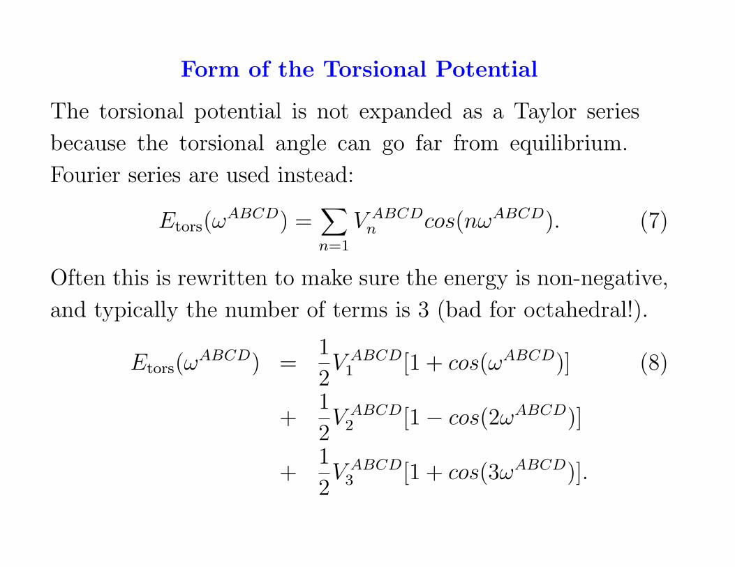
Form of the Torsional Potential

The torsional potential is not expanded as a Taylor series

because the torsional angle can go far from equilibrium.

Fourier series are used instead:

Etors(ωABCD) =

∑

n=1

V ABCDn cos(nωABCD). (7)

Often this is rewritten to make sure the energy is non-negative,

and typically the number of terms is 3 (bad for octahedral!).

Etors(ωABCD) =

1

2V ABCD1 [1 + cos(ωABCD)] (8)

+1

2V ABCD2 [1− cos(2ωABCD)]

+1

2V ABCD3 [1 + cos(3ωABCD)].

For a molecule like ethylene, rotation about the C=C bond

must be periodic by 180o, so only even terms n = 2, 4, . . . can

occur. For a molecule like ethane, only terms n = 3, 6, 9, . . .

can occur.

Figure 4: Torsional Potentials for n = 3 and 2 (Jensen)

Figure 5: Example Torsional Potential for n = 1 (Jensen)

van der Waals Energy

The van der Waals energy arises from the interactions between

electron clouds around two nonbonded atoms.

Short range: strongly repulsive

Intermediate range: attractive

Long range: goes to zero

The attraction is due to electron correlation which results in

“dispersion” or “London” forces (instantaneous multipole /

induced multipole).

Form of the van der Waals Energy

van der Waals energies are usually computed for atoms which

are connected by no less than two atoms (e.g., 1-4 interactions

between A and D in A-B-C-D and higher). Interactions betwen

atoms closer than this are already accounted for by stretching

and/or bending terms.

At intermediate to long ranges, the attraction is proportional

to 1/R6. At short ranges, the repulsion is close to exponential.

Hence, an appropriate model of the van der Waals interaction

is

Evdw(RAB) = Ce−DR − E

R6. (9)

Since the van der Waals and electrostatic interactions are

long-range, they can become the dominant costs of force-field

computation. The van der Waals term can be speeded up

substantially by a more economical expression, the Lennard-

Jones potential

Evdw(RAB) = ǫ

[

(

R0

R

)12

− 2(

R0

R

)6]

. (10)

The R−12 term is easier to compute than the exponential

because no square roots need to be taken to get R. Figure 6

presents a comparison of various van der Waals potentials.

Figure 6: Example van der Waals Potentials (Jensen)

Electrostatic Energy

Electrostatic terms describe the Coulomb interaction between

atoms A and B with partial charges (e.g., in carbonyls),

according to

Eel(RAB) =

QAQB

ǫRAB, (11)

where ǫ is an effective dialectric constant which is 1 in vacuum

but higher when there are intermediate atoms or solvent.

Usually ǫ is picked fairly arbitrarily; higher values or so-called

“distance-dependent dialectrics” (ǫ = ǫ0RAB) account for

“screening” and kill off the electrostatic contributions faster,

making them easier to compute.

Alternative Approaches to Electrostatics

A slightly different approach to partial charges is to consider

polarized bonds as dipoles, and compute the electrostatic

interaction between these dipoles (e.g., MM2 and MM3):

Eel(RAB) =

µAµB

ǫ(RAB)3(cosχ− 3 cosαAcosαB) , (12)

where χ is the angle between the dipoles and αA and αB are

the angles each dipole makes with the line joining atoms A and

B.

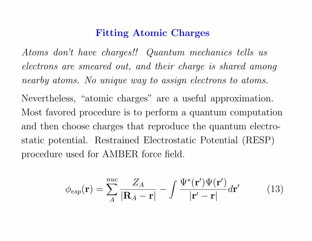
Fitting Atomic Charges

Atoms don’t have charges!! Quantum mechanics tells us

electrons are smeared out, and their charge is shared among

nearby atoms. No unique way to assign electrons to atoms.

Nevertheless, “atomic charges” are a useful approximation.

Most favored procedure is to perform a quantum computation

and then choose charges that reproduce the quantum electro-

static potential. Restrained Electrostatic Potential (RESP)

procedure used for AMBER force field.

φesp(r) =nuc∑

A

ZA

|RA − r| −∫ Ψ∗(r′)Ψ(r′)

|r′ − r| dr′ (13)

Computational Cost of Electrostatic Terms

Like van der Waals terms, electrostatic terms are typically

computed for nonbonded atoms in a 1,4 relationship or further

apart. They are also long range interactions and can dominate

the computation time.

The number of nonbonded interactions grows quadratically

with molecule size. The computation time can be reduced by

cutting off the interactions after a certain distance. The van

der Waals terms die off relatively quickly (∝ R−6) and can

be cut off around 10 A. The electrostatic terms die off slower

(∝ R−1, although sometimes faster in practice), and are much

harder to treat with cutoffs. This is a problem of interest to

developers.

Improved Electrostatic Energies

The point-charge model has serious deficiencies: (a) electro-

static potentials are not accurately reproduced; (b) simple

models don’t allow the charges to change as the molecular ge-

ometry changes, but they should; (c) only pairwise interactions

are considered, but an electrostatic interaction can actually

change by ∼10-20% in the presence of a third body (induction

or “polarization” effects).

Improved Electrostatic Potentials

Electrostatic potentials can be more accurately reproduced by:

• Allowing non-atom-centered charges

• Adding point dipoles, quadrupoles, etc.

Both are employed in Anthony Stone’s Distributed Multipole

Analysis (DMA). However, this does not yet allow the elec-

trostatic variables to change as a function of geometry or to

respond to electrostatic potentials generated by nearby atoms.

This requires polarizable force-fields such as the fluctuating

charge model.

The Fluctuating Charge Model

Consider the energy as a function of the number of electrons

N :

E = E0 +∂E

∂N∆N +

1

2

∂2E

∂N2(∆N)2 + · · · (14)

Electronetativity χ = −∂E/∂N . Chemical hardness η =

∂2E/∂N2. Setting ∆Q = −∆N and expanding about the

point with no net atomic charges,

E = χQ+1

2ηQ2 + · · · (15)

Considering the electrostatic energy also depends on the

external potential φ, and summing over all sites (usually

atomic centers),

Eel =∑

A

φAQA +∑

A

χAQA +1

2ηABQAQB. (16)

In vector notation, and requiring that the energy be stationary

with respect to the charges with and without an external

potential,

∂E

∂Q|φ 6=0 = φ+ χ+ ηQ = 0 (17)

∂E

∂Q|φ=0 = χ+ ηQ0 = 0 (18)

which yields

∆Q = −η−1φ, (19)

where φ depends on the charges at all sites (and thus the

equations must be solved iteratively),

φ(r) =∑

A

QA

|r−RA|. (20)

Other Polarizable Models

The fluctuating charge model has some limitations. More

general models incorporate explicit polarizability terms. A

dipole moment can result from a polarization of the electronic

charge as a result of an electric field (F = ∂φ/∂r):

µind = αF (21)

Epolel =

1

2µindF =

1

2αF2 (22)

It is common to break up the polarizability α into “atomic

polarizability” contributions.

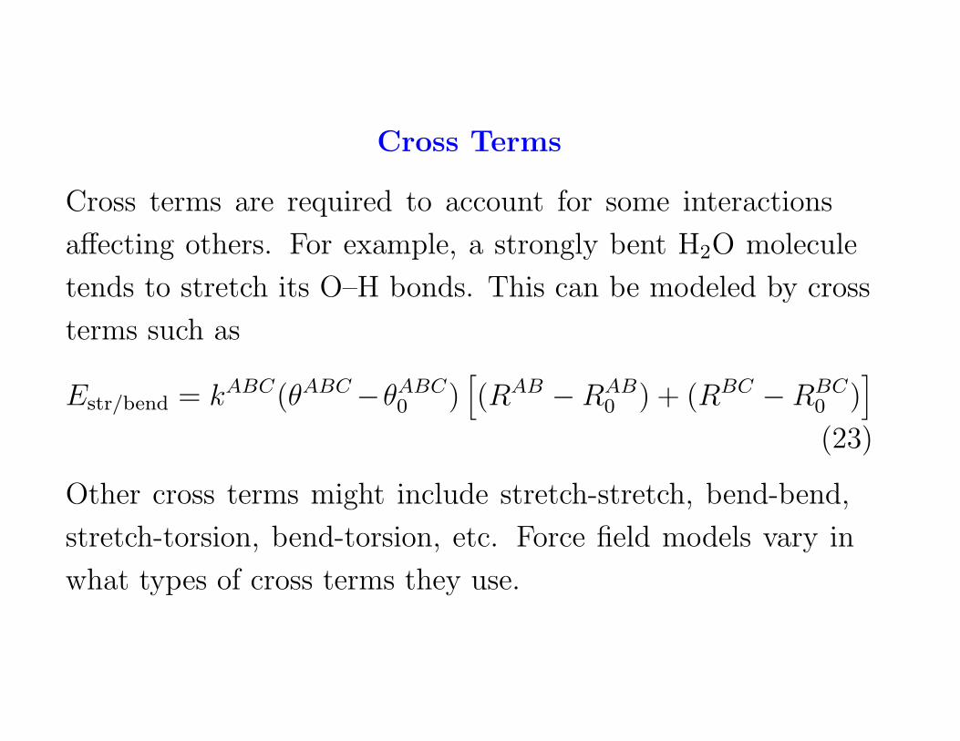
Cross Terms

Cross terms are required to account for some interactions

affecting others. For example, a strongly bent H2O molecule

tends to stretch its O–H bonds. This can be modeled by cross

terms such as

Estr/bend = kABC(θABC−θABC0 )

[

(RAB −RAB0 ) + (RBC −RBC

0 )]

(23)

Other cross terms might include stretch-stretch, bend-bend,

stretch-torsion, bend-torsion, etc. Force field models vary in

what types of cross terms they use.

Parameterizing the Force Fields

Molecular mechanics requires many parameters, e.g., RAB0 ,

kAB, θABC0 , kABC , V ABCD

n , etc. Assuming there are 30 atoms

which form bonds with each other, there are 304/2 torsional

parameters for each V ABCDn term, or 1 215 000 parameters

for V1 through V3! Only the 2466 “most useful” torsional

parameters are present in MM2, meaning that certain torsions

cannot be described.

Lack of parameters is a serious drawback of all force field

methods. Automatic guessing of unavailable parameters is

sometimes done but is very dangerous.

Heats of Formation

∆Hf is the heat conent relative to the elements at standard

state at 25o C (g). This is a useful quantity for comparing

the energies of two conformers of a molecule or two different

molecules.

Bond energy schemes estimate the overall ∆Hf by adding

tabulated contributions from each type of bond. This works

acceptably well for strainless systems.

Molecular mechanics adds steric energy to the bond/structure

increments to obtain better estimates of ∆Hf .

The bare molecular mechanics energy is not a meaningful

quantity for comparing different molecules.

Accuracy of Heats of Formation

In principle, other corrections should be added (but usually

are not): population increments (for low-lying conformers),

torsional increments (for shallow wells), and corrections for low

(< 7 kcal/mol) barriers other than methyl rotation (already

included in group increment).

The performance of the MM2 force field for typical molecules

is given in Table 1. Overall, these results are rather good;

however, unusual molecules can exhibit far larger errors.

Table 1: Average errors in heat of formations (kcal/mol) by

MM2a

Compound type Avg error ∆Hf

Hydrocarbons 0.42

Ethers and alcohols 0.50

Carbonyls 0.81

Aliphatic amines 0.46

Aromatic amines 2.90

Silanes 1.08

aTable 2.6 from Jensen’s Introduction to Computational Chem-

istry.

Different Force Field Methods

Class I Methods: Higher order terms and cross terms. Higher

accuracy, used for small or medium sized molecules. Examples:

Allinger’s MM1-4, EFF, and CFF.

Class II Methods: For very large molecules (e.g., proteins).

Made cheaper by using only quadratic Taylor expansions

and neglecting cross terms. Examples: AMBER, CHARMM,

GROMOS, etc. Made even cheaper by using “united atoms.”

Hybrid Force Field/Electronic Structure Methods

Treat “uninteresting” parts of the molecule by force field

methods and “interesting” parts by high-accuracy electronic

structure methods. This approach is useful for systems

where part of the molecule is needed at high accuracy or for

which no force field parameters exist (e.g., metal centers in

metalloenzymes).

Examples: Morokuma’s ONIOM method; QM/MM methods.

QM/MM Approaches

Etotal = EQM + EMM + EQM/MM (24)

• Mechanical embedding: Include bonded and steric inter-

actions between QM and MM regions, and maybe assign

partial charges to the QM atoms

• Electronic embedding: Also add partial charges on MM

atoms to QM computation

• Polarizable embedding: Also allow QM atoms to polarize

MM region (only applies to polarizable force fields or

Gordon’s effective fragment method)

If the QM/MM boundary cuts covalent bonds, dangling bonds

are terminated by so-called “link atoms” (typically hydrogen).

Morokuma’s ONIOM Approach

ONIOM: Our Own n-Layered Integrated Molecular Orbital

Molecular Mechanics Method

EONIOM(real system, high level) = Elow level(real system)

+ Ehigh level(model system)

− Elow level(model system)

Can also involve multiple layers. Originally used only mechan-

ical embedding for the QM/MM interface, but more recently

uses electronic embedding. Can also do as a QM/QM with

high and low levels of quantum mechanics.