J Sched (2009) 12: 281–298DOI 10.1007/s10951-008-0079-3

Scheduling projects with multi-skilled personnel by a hybridMILP/CP benders decomposition algorithm

Haitao Li · Keith Womer

Received: 1 May 2007 / Accepted: 4 July 2008 / Published online: 3 September 2008© Springer Science+Business Media, LLC 2008

Abstract We study an assignment type resource-con-strained project scheduling problem with resources beingmulti-skilled personnel to minimize the total staffing costs.We develop a hybrid Benders decomposition (HBD) algo-rithm that combines the complimentary strengths of bothmixed-integer linear programming (MILP) and constraintprogramming (CP) to solve this NP-hard optimization prob-lem. An effective cut-generating scheme based on temporalanalysis in project scheduling is devised for resolving re-source conflicts. The computational study shows that ourhybrid MILP/CP algorithm is both effective and efficientcompared to the pure MILP or CP method alone.

Keywords Resource-constrained project scheduling ·Multi-skilled personnel · Hybrid MILP/CP algorithms ·Benders decomposition

1 Introduction

Scheduling and assignment of multi-skilled personnel toperform a project is of practical importance, as cross-training is becoming an viable practice to save operationscosts and to justify technology investment in many organi-zations, e.g., call centers (Aksin et al. 2006). We considerthe following project scheduling problem with multi-skilledpersonnel as resource constraints. A project consists of aset of tasks which must be completed by a given deadline.

H. Li (�) · K. WomerCollege of Business Administration, University of Missouri—St. Louis, One University Blvd., St. Louis, MO 63121, USAe-mail: lihait@umsl.edu

K. Womere-mail: womerk@umsl.edu

Generalized temporal constraints include due dates, min-imum and maximum time lags. (A precedence constraintcan be viewed as a special case of a minimum time lagconstraint.) The project involves a set of skills. Each taskmay require multiple skills simultaneously in order for thetask to progress. Each skill requires one individual selectedfrom a pool of personnel that possess the skill. An individ-ual may be able to perform multiple skills, but only one ata time. The assigned workload for each person cannot ex-ceed the individual’s maximum workload capacity duringthe scheduling horizon. The objective is to minimize thestaffing costs subject to the generalized temporal relations,resource constraints, and the deadline on the project com-pletion time (makespan). As a generalization of the single-mode resource constrained project scheduling (RCPSP), theproject scheduling problem with multi-skilled personnel isstrongly NP-hard.

We develop a hybrid mixed-integer linear programming(MILP) and constraint programming (CP) solution approachrelying on the classical Benders decomposition (Benders1962) for handling complex mixed-integer programs. Theoriginal project scheduling problem with multi-skilled per-sonnel is decomposed into a relaxed master problem (RMP)containing only the assignment variables and constraints,and a feasibility subproblem containing only the schedulingvariables and constraints. CP is used for solving the schedul-ing subproblem to infer “cuts” that are added iteratively intothe RMP to exclude infeasible assignments. MILP methodssuch as branch–and–bound and branch–and–cut are used tosolve the master problem. Such a hybrid Benders decom-position (HBD) framework was first proposed by Jain andGrossmann (2001) to solve a class of scheduling problemsimilar to the open-shop multi-purpose machine (OMPM,Brucker 2001) scheduling problem, where temporal con-straints are restricted to release- and due-date constraints

282 J Sched (2009) 12: 281–298

and only the general “no-good” cuts are generated during thesolving process. Due to the generality and complexity of ourproposed problem, we devise a cut-generating scheme basedon temporal analysis in project scheduling to establish a linkbetween the assignment master problem and scheduling sub-problem. This insight is the key to the practical effectivenessand efficiency of our algorithm.

In general, the model and solution approach presentedin this paper can be used in two ways. First, with the per-sonnel’s skill-mix given, the model optimizes the short-term assignment and scheduling decisions for accomplish-ing projects. Second, with the personnel’s skill-mix un-known, the model can be used to obtain an optimal skill-mix of personnel for planning decisions in the intermediate-term. We refer to Li and Womer (2006a) for an applicationof determining the optimal crew composition and reducingcrew size.

The paper is organized as follows. Section 2 introducesthe project scheduling problem with multi-skilled person-nel and presents its MILP formulation. Section 3 providesan introduction to constraint programming and surveys thehybrid MILP/CP approaches in the current literature. InSect. 4, we develop our hybrid MILP/CP Benders decompo-sition algorithm for solving the proposed problem. Section 5presents the computational results. In Sect. 6, we examinethe relationship between our model/algorithm and planningproblems. Section 7 gives conclusions and discusses futureresearch opportunities.

2 Project scheduling with multi-skilled personnel

In this section, we first describe the project scheduling prob-lem with multi-skilled personnel and provide an illustrativeexample. We then present MILP formulation of the problemwhich our decomposition algorithm depends on. Additionalremarks are made on the related models and past work.

2.1 Problem description

We let J be the set of tasks in the project, K be the set ofrelevant skills and S the personnel set required for executingthe project. The set of skills required by task j is denotedby Kj . The set of people who are able to perform skill k isrepresented by Sk . Each skill must be assigned to one personwho is able to perform that skill. Each task j has a constantprocessing time pj . The minimum delay between task j andj ′ is δjj ′ , i.e., task j ′ cannot start until δjj ′ time units afterj starts. The due date for task j is dj . There is a work loadcapacity of ws for each individual s ∈ S. The deadline on themakespan of the project is T̄ . The objective is to minimizethe total staffing costs to perform the project given a salaryof cs paid to an individual s ∈ S. We additionally make thefollowing assumptions:

(A1) Simultaneous skill requirement: the required skillsmust be present simultaneously for a task to progress.

(A2) Single skill performance: personnel are treated asunary resources, meaning an individual can only per-form one skill at each time point.

(A3) A task cannot be interrupted, i.e., no preemption is al-lowed.

(A4) Setup times are not considered explicitly.

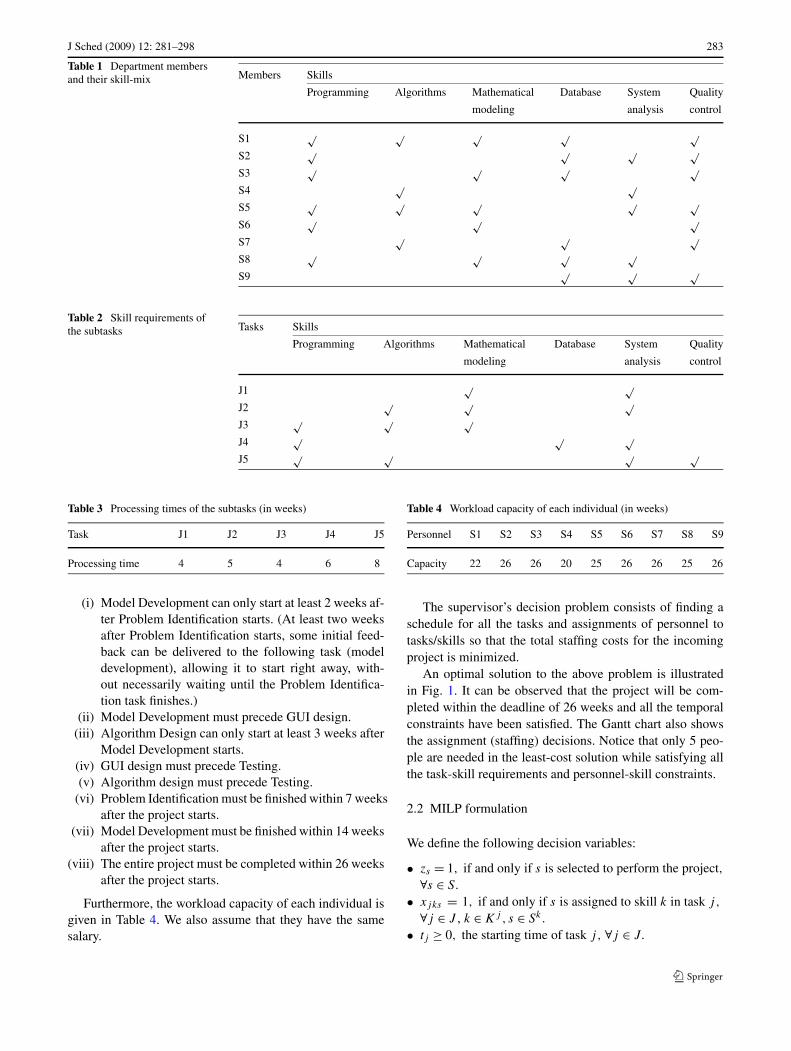
We present a numerical example to illustrate the projectscheduling problem with multi-skilled personnel. The soft-ware development department in a small firm faced ascheduling problem involving skilled labor. In the past, thedepartment operated as a job shop with projects (jobs) ar-riving at irregular intervals with varying work requirements.But the department supervisor soon found it necessary toremodel the operational process to improve efficiency. Sixcategories of skills are needed for the department members:programming, algorithms, mathematical modeling, data-base, systems analysis, and quality control. Staff membersin the department are all cross-trained and possess multi-ple skills. But an individual can only perform one skill atone time point. Projects arrived with varying requirementsfor skills and could be broken down into subtasks. Table 1outlines members in the department and their skill-mix.

An upcoming project is to develop software for the ABCCompany. It can be broken down into five tasks, each ofwhich requires a specific set of skills simultaneously for thetask to progress. The skill requirements of the project arepresented in Table 2.

Additional descriptions of the tasks are provided below:

(J1) Problem identification. It defines the problem faced bythe client while considering the technical capacity ofthe developing group.

(J2) Model development. It sets up the underlying mathe-matical programming model for identified optimizationproblem.

(J3) Algorithm design. It develops algorithms for solvingthe proposed model.

(J4) GUI design. It designs a user-friendly interface allow-ing easy accessibility.

(J5) Testing. It includes testing and debugging the applica-tion software to assure quality.

Table 3 gives the processing time of each task.Considering the technical requirements among these

tasks, the department supervisor believed that project make-span could be significantly shortened if generalized tem-poral constraints are introduced in addition to the currentsimple precedence relations as in the job shop schedulingenvironment. This is achieved by allowing simultaneouslyexecutions of some tasks (e.g., the minimal time lags). Thetemporal constraints he can think of are listed below:

J Sched (2009) 12: 281–298 283

Table 1 Department membersand their skill-mix Members Skills

Programming Algorithms Mathematical Database System Quality

modeling analysis control

S1 √ √ √ √ √S2 √ √ √ √S3 √ √ √ √S4 √ √S5 √ √ √ √ √S6 √ √ √S7 √ √ √S8 √ √ √ √S9 √ √ √

Table 2 Skill requirements ofthe subtasks Tasks Skills

Programming Algorithms Mathematical Database System Quality

modeling analysis control

J1 √ √J2 √ √ √J3 √ √ √J4 √ √ √J5 √ √ √ √

Table 3 Processing times of the subtasks (in weeks)

Task J1 J2 J3 J4 J5

Processing time 4 5 4 6 8

(i) Model Development can only start at least 2 weeks af-ter Problem Identification starts. (At least two weeksafter Problem Identification starts, some initial feed-back can be delivered to the following task (modeldevelopment), allowing it to start right away, with-out necessarily waiting until the Problem Identifica-tion task finishes.)

(ii) Model Development must precede GUI design.(iii) Algorithm Design can only start at least 3 weeks after

Model Development starts.(iv) GUI design must precede Testing.(v) Algorithm design must precede Testing.

(vi) Problem Identification must be finished within 7 weeksafter the project starts.

(vii) Model Development must be finished within 14 weeksafter the project starts.

(viii) The entire project must be completed within 26 weeksafter the project starts.

Furthermore, the workload capacity of each individual isgiven in Table 4. We also assume that they have the samesalary.

Table 4 Workload capacity of each individual (in weeks)

Personnel S1 S2 S3 S4 S5 S6 S7 S8 S9

Capacity 22 26 26 20 25 26 26 25 26

The supervisor’s decision problem consists of finding aschedule for all the tasks and assignments of personnel totasks/skills so that the total staffing costs for the incomingproject is minimized.

An optimal solution to the above problem is illustratedin Fig. 1. It can be observed that the project will be com-pleted within the deadline of 26 weeks and all the temporalconstraints have been satisfied. The Gantt chart also showsthe assignment (staffing) decisions. Notice that only 5 peo-ple are needed in the least-cost solution while satisfying allthe task-skill requirements and personnel-skill constraints.

2.2 MILP formulation

We define the following decision variables:

• zs = 1, if and only if s is selected to perform the project,∀s ∈ S.

• xjks = 1, if and only if s is assigned to skill k in task j,

∀j ∈ J , k ∈ Kj , s ∈ Sk.

• tj ≥ 0, the starting time of task j, ∀j ∈ J.

284 J Sched (2009) 12: 281–298

Fig. 1 Gantt chart of an optimalsolution to the example problem

• yjj ′ = 1, if and only if task j precedes j ′, ∀(j, j ′) ∈J × J .

The MILP formulation of the project scheduling problemwith multi-skilled personnel can be written as:

min∑

s∈S

cszs (1)

subject to:∑

s∈Sk

xjks = 1, ∀j ∈ J, k ∈ Kj ; (2)

∑

k∈Kj

xjks ≤ 1, ∀j ∈ J, s ∈ S; (3)

∑

j∈J

∑

k∈Kj

pjxjks ≤ wszs, ∀s ∈ S; (4)

tj ′ − tj ≥ δjj ′ , ∀(j, j ′) ∈ J × J ; (5)

tj + pj ≤ min{dj , T̄ }, ∀j ∈ J ; (6)

yjj ′ + yj ′j ≥ xjks + xj ′k′s − 1,

∀ ordered (jk, j ′k′), ∀s ∈ S; (7)

tj ′ ≥ tj + pj − M(1 − yjj ′), ∀j �= j ′; (8)

zs, xjks, yjj ′ ∈ {0,1};tj ≥ 0.

The objective function (1) minimizes the total staffingcosts for executing the project. Constraints (2) through (4)model the assignment aspect of the problem. Constraint (2)states that each skill in a task requires one person who pos-sesses that skill. Constraint (3) enforces that no individual isassigned to more than one skill in the same task due to as-sumptions (A1) and (A2). Constraint (4) ensures that the to-tal assigned workload of each person cannot exceed his/herworkload capacity. Constraints (5) through (8) take care ofthe generalized temporal relations, i.e., the scheduling as-pect of the problem. When δjj ′ ≥ 0, constraint (5) repre-sents a minimum time lag between task j and j ′; whenδjj ′ < 0, (5) represents a maximum time lag between task

j ′ and j ; when δjj ′ = pj , (5) reduces to a precedence con-straint. Constraint (6) satisfies the due date of each task aswell as the deadline on the makespan. Constraint (7) statesthe logic relationship between sequencing and assignmentvariables, i.e., if two tasks are assigned with the same personthen these two tasks cannot overlap (one sequencing relationmust be determined) due to assumption (A2). Constraint (8)is the classical big-M formulation in disjunctive program-ming to define the sequencing variables. For a two-layer re-source structure to characterize the problem, we refer to Liand Womer (2006b).

2.3 Additional remarks

The project scheduling problem with multi-skilled per-sonnel studied in this paper is a generalization of thesingle-mode resource-constrained project scheduling prob-lem (RCPSP) by allowing each task to be performed in mul-tiple ways. We refer to Brucker et al. (1999) for a surveyof various RCPSP models. It also belongs to the assign-ment type RCPSP (Drexl et al. 1998) due to the presenceof both the assignment and sequencing variables. It is sim-ilar to the multi-mode RCPSP in that each task has mul-tiple ways (modes) to be performed. To be specific, fortask j there are

∏k∈Kj |Sk| ways to be considered, which

makes the problem size increase explosively if modeled bya standard multi-mode RCPSP. It is also an extension of themulti-purpose machine scheduling problem (MPM, Brucker2001), due to the presence of the generalized temporal con-straints (5) in addition to the usual precedence constraintsin the classical machine scheduling problems. This paperextends the work of Li and Womer (2006b) by minimizingthe total staffing cost instead of the number of selected per-sonnel. This is not a trivial generalization; we will show inSect. 3.2 that the Skill-Level Based Decomposition (SLBD)algorithm proposed by Li and Womer (2006b) will not beable to handle the objective function considering the cost ofselecting each individual.

Other work on project scheduling problems with multi-skilled personnel include Focacci et al. (2000), Bellenguezand Neron (2004) and Neron et al. (2006). Their models,however, treat a set of personnel merely as unary resources,

J Sched (2009) 12: 281–298 285

while the capacity associated with each individual was notconsidered. In addition, temporal constraints in their stud-ies are restricted to precedence constraints, i.e., minimum ormaximum time lag is not considered. Moreover, they all seekto minimize the project makespan instead of cost-related ob-jective functions.

3 CP-based hybrid approaches

3.1 Constraint programming

Constraint programming is the study of computational sys-tems based on constraints. It originated in the Artificial In-telligence areas that investigate the Constraint SatisfactionProblem (CSP, Tsang 1993) and Logic Programming (VanHentenryck 1999). The main solving technologies of CP in-clude constraint propagation and search. The basic idea ofconstraint propagation is that when a variable’s domain ismodified, the effects of this modification are then commu-nicated to any constraint that interacts with that variable.In other words, the domain reduction algorithm modifiesthe domain of all the variables in that constraint, given themodification of one of the variables in that constraint. Werefer to Tsang (1993) for a detailed description of variousgeneral-purpose constraint propagation algorithms and Bap-tiste et al. (2001) for efficient constraint propagation algo-rithms for scheduling problems. The domain of each vari-able in an optimization problem can be reduced throughconstraint propagation. However, reducing a problem to aminimum problem, i.e., no more redundant values can beremoved from the domain of the problem is often NP-hard.This is why a search procedure is often needed to explorethe remaining solution space. Most popular search strategiesinclude depth-first (DF), best-first (BF), and limited discrep-ancy search (LDS, Harvey and Ginsberg 1995).

The CP techniques can be compared and contrasted withMILP. Hooker (2002) pointed out that the differences andcomplementary strengths between the two techniques indi-cate the opportunity for integrating; while the commonali-ties often make the integration natural and easier. Two areasof differences can be observed between CP and MILP.

First, from the modeling perspective CP’s declarative na-ture can make the model expressive and compact with fewervariables and constraints when compared with the MILP for-mulation. This is especially true when modeling schedulingproblems. In most of the CP software such as ILOG Solver(ILOG 2002a), ECLiPSe (Wallace et al. 1997), and CHIP(Dincbas et al. 1988), there are special constructs availableto model scheduling constraints in an expressive and com-pact way. In contrast, the modeling power of MILP has beengreatly hampered by the restrictiveness of linear expressionsfor handling the temporal and resource constraints encoun-tered in scheduling problems. The disjunctive formulation

of these constraints often involves an explosive number ofchoice variables and constraints as evident in constraint (7)and (8) in Sect. 2.2

Second, from the algorithmic perspective CP solves anoptimization problem through a naïve branch–and–boundmethod by gradually tightening a bound on the objectivefunction. For a minimization problem with an objectivefunction f (x), each time a feasible solution x̄ is found, aconstraint f (x) < f (x̄) is added to the constraint store ofeach subproblem in the remaining search tree. It is not ef-ficient to do this in practice, since there is no sophisticatedrelaxation algorithm in CP to obtain tight bounds and thelink between the objective function and the decision vari-ables is quite loose (Milano and Trick 2004). In MILP, how-ever, various relaxation methods have been well developed(Nemhauser and Wolsey 1988). Hence, the success of CPdepends largely on the effectiveness of constraint propaga-tion; whilst in MILP, the quality of relaxation plays an im-portant role. Thus, the solution procedure may benefit fromincorporating bounding information obtained by relaxationstechniques in MILP to prune the solution space and accel-erate search. Sometimes a problem has some characteris-tics better handled by CP while others are better handled byMILP. For such problems neither MILP nor CP alone mayperform well.

3.2 Hybrid approaches

Various integration schemes have been proposed to take ad-vantage of the complementary strengths of CP and MILPfor solving combinatorial optimization problems. Theseschemes can be generally classified into two categories:preprocessing and hybrid approaches. Constraint propaga-tion has been used as a preprocessing tool to reduce theproblem size of an RCPSP by Brucker and Knust (1998).CP-based lower bounds for both the single-mode and multi-mode RCPSP have also been studied by Brucker and Knust(2000, 2003).

As for hybrid approaches, Bockmayr and Kasper (1998)presented a unifying framework called branch–and–infer,in which constraints for both MILP and CP are dividedinto two categories, primitive and non-primitive. They dis-cussed how non-primitive constraints could be used to inferprimitive constraints. Hooker and Osorio (1999) proposeda mixed logic/linear modeling framework which is furthertreated in detail by Hooker (2002). Hybrid approaches of-ten depend on decompositions and allow close communi-cations between the MILP and CP solvers. Different hy-brid decomposition schemes include CP-based branch–and–price (Easton et al. 2004), CP based Lagrangian relaxation(Benoist et al. 2001 and Sellmann and Fahle 2003) andCP-based Benders decomposition (Benoist et al. 2002 andEremin and Wallace 2001). Notably, Jain and Grossmann

286 J Sched (2009) 12: 281–298

(2001) proposed a hybrid Benders decomposition (HBD)algorithm to solve a class of scheduling problem similarto the open-shop multi-purpose machine (OMPM, Brucker2001) scheduling problem, where temporal constraints arerestricted to release- and due-date constraints. The com-putational results on the same problem were improved byThorsteinsson (2001) through a framework called branch–and–check where the master problem is not solved to opti-mality but halts once a feasible solution is found, and grad-ually tightens the objective function value. Jain and Gross-mann’s cut-generating scheme relies largely on the fact thatresource units (machines) are independent in the OMPM, sothat cuts could be generated for each individual machine in-dependently. For more general scheduling problems, such asthe project scheduling problem with multi-skilled personnelstudied in this paper, it is not possible to infer cuts for eachperson independently as the skilled personnel are interre-lated through precedence or time lag constraints. In addi-tion, the cuts generated by Jain and Grossmann (2001) aresimple “no-good” cuts, which could be rather weak whenthey correspond with the entire set of resource units. It isa challenge to infer effective cuts when resource units areinterrelated with each other. According to the authors’ bestknowledge, the HBD approach has not be implemented onsolving scheduling problems with precedence or time lagconstraints.

Li and Womer (2006b) developed a combined MILP/CPdecomposition heuristic called Skill Level Based Decompo-sition (SLBD) to heuristically solve a similar problem withthe objective function minimizing the number selected ofpersonnel. The SLBD works in such a way that a schedul-ing subproblem is solved first to obtain a feasible schedule,followed by a resource leveling procedure that smoothes theresource utilization, and finally an assignment problem issolved to obtain a feasible solution to the original problem.The skill level, i.e., the skill availability for the schedulingsubproblem, is controlled as low as possible to obtain a fea-sible schedule for the succeeding assignment phase. A moreelaborate procedure based on tabu search was implementedby Li and Womer (2006a) in the resource leveling phase tosmooth the resource utilization. However, since the objec-tive function (1) may not be a monotonic function of thenumber of selected personnel, the SLBD is unable to handlethe objective function with staffing costs considered in thispaper, although it has shown significant advantages over thepure MILP or CP approach alone in both solution qualityand speed.

4 The hybrid Benders decomposition algorithm

4.1 Hybrid Benders decomposition

The classical Benders decomposition (Benders 1962) is amethod for solving optimization problems with enormous

numbers of constraints. As the dual of the column genera-tion method, the strategy here is to generate rows or con-straints and successively add them into the constraint sys-tem. Cuts (constraints) generated based on duality theory arecalled “Benders cuts”.

Following the hybrid MILP/CP Benders decomposi-tion (HBD) framework by Jain and Grossmann (2001), wedecompose the original project scheduling problem withskilled-personnel into a relaxed master problem (RMP),which contains only assignment decision variables, and afeasibility subproblem (SP) which takes care of the schedul-ing aspect of the problem. We rely on MILP methods such asbranch–and–bound and branch–and–cut to solve the RMP.We use CP to model the scheduling SP which would oth-erwise be difficult for MILP to model and apply CP-basedalgorithms to solve the feasibility scheduling SP, for whichefficient constraint propagation algorithms are available.

We let the assignment binary variable xijk and selec-tion binary variable zs be associated with the RMP. Therest of the variables related to the scheduling part of theproblem, i.e., the starting time of each task tj and the se-quencing variable yjj ′ will be replaced by CP variables toconstruct the scheduling subproblem. All the submodels areconstructed in OPL, a modeling language supporting bothlinear programming and constraint programming (Van Hen-tenryck 1999).

The MILP formulation of the RMP at iteration n can bewritten as:

RMP_MILP(n)

= {min

∑

s∈S

cszs

subject to:

constraints (2), (3), and (4)

βi(X) ≤ 1, ∀i = 1, . . . , n. (9)

}

Constraints (9) include cuts generated at each iteration i.Each cut prevents a pair of overlapping activities from be-ing assigned to the same individual. The overlapping ac-tivities are identified through temporal analysis techniquesin project scheduling, which will be explained in detail inSect. 4.3.

For a partial solution (Xn,Zn) from solving the RMPat iteration n, we define a scheduling feasibility subprob-lem modeled by CP. By fixing the assignment variables(Xn,Zn), the subproblem SP decides if this partial solutioncan be extended to a complete solution. We define the set ofavailable personnel S as an array of unary resources called

J Sched (2009) 12: 281–298 287

SkilledPersonnel:

UnaryResource SkilledPersonnel [S].Then the CP formulation of the feasibility SP at iteration n

can be written as below, where the italic words are keywordsin OPL

SP_CP(n)

= {Solve

subject to:

j precedes j ′, ∀(j, j ′) ∈ P ; (10)

j.start + δjj ′ ≤ j ′.start, ∀(j, j ′) ∈ J × J\P ;(11)

j.start + pj ≤ min{dj , T̄ }, ∀j ∈ J ; (12)

if xijks = 1, then j requires SkilledPersonnel[s],

∀i = 1, . . . , n; j ∈ J, k ∈ Kj , s ∈ S. (13)

}Constraints (10) through (12) take care of the tempo-

ral constraints. CP provides a descriptive way to expressthe precedence constraint as in (10), where P representsthe set of precedence constraints. Constraints (11) and (12)are equivalent with (5) and (6), respectively, where j.startrefers to the starting time of activity j . Constraint (13) es-tablishes the link between assignment variables and resourceconstraints. Since the values of xi

jks are fixed through solv-ing the RMP_MILP(i) at iteration i, i.e., the assignmentof tasks/skills to the skilled personnel has been made, theoriginal complex assignment-type scheduling problem re-duces to a pure single-mode RCPSP with unary resourcesfor which efficient constraint propagation algorithms exist(Baptiste et al. 2001). Also notice that comparing with thepure CP formulation in Li and Womer (2006b), here an ac-tivity is defined at the task level instead of the skill level,hence the number of activities in the subproblem has beenreduced. In addition, SP_CP(n) is a feasibility problem in-stead of an optimization problem. That is, it only needs todetermine whether a feasible solution exists or not, a prob-lem for which CP is relatively efficient to handle.

The way to generate cuts is often the key to success ofa Benders decomposition algorithm. A main feature of ourHBD is to obtain the possible causes of infeasibility ex ante,i.e., before the main algorithm iterations start. The role ofsolving the scheduling subproblem is to infer (trigger) theviolated constraints. The causes of infeasibility to the sub-problem can be interpreted a priori as “two overlapping ac-tivities are assigned to the same individual” due to assump-tion (A2). Theoretically, we could obtain all pairs of over-lapping activities and include the complete set of constraints

(9) in the RMP. However, it is impractical to do so becauseof the enormous number of such constraints and also the factthat only a small fraction of such constraints are binding atan optimal solution (Lasdon 1970). Hence, the causes of in-feasibility are inferred as cuts, which are added iterativelyinto the RMP. Next we describe our cut generating schemesin detail.

4.2 Generating cuts

We first introduce the concept of minimal forbidden set inthe resource-constrained project scheduling literature. A for-bidden set represents a set of activities whose total require-ment for some resource exceeds the available capacity of theresource (Bartusch et al. 1988). A set of activities F ⊆ A iscalled a forbidden set if∑

j∈F

rjk > Qk for some k ∈ R,

where R refers to the set of resources, Qk refers to theavailable capacity of resource k, and rjk denotes the re-quirement of resource k by activity j . If no proper sub-set F ′ ⊂ F is forbidden, we call F a minimal forbiddenset. For a unary resource such as each individual s ∈ S inour model, a minimal forbidden set always contains two el-ements, e.g., Fs = {j, j ′|s is assigned to both j and j ′}. Toresolve the resource conflicts caused by Fs , a precedenceconstraint j precedes j ′ (or j ′ precedes j) needs to be in-troduced to “break up” Fs (to prevent j and j ′ from beingexecuted simultaneously). We have the following observa-tions concerning the resulting scheduling problem with thenewly added precedence constraint:

Observation 1 When j and j ′ must overlap in order to sat-isfy the temporal constraints (3) and (4) (denoted by j‖j ′),the resulting scheduling problem will not be feasible.

Observation 2 When j and j ′ never overlap in order to sat-isfy the temporal constraints (3) and (4) (denoted by j ∼ j ′),the resulting scheduling problem will always be feasible.

Observation 3 When neither (O1) nor (O2) occurs, i.e., j

and j ′ are possible to overlap (denoted by j |j ′), the result-ing scheduling problem may or may not be feasible.

Observation 1 indicates that the only way to resolve in-feasibility is to prevent j and j ′ from being assigned withthe same person, which generates a valid cut (global cut) forthe RMP. Observation 2 implies that no cut will be gener-ated (or generating a redundant cut) for the RMP, as it isalways feasible to assign the same person to j and j ′. Eventhough the cut generated through Observation 3 may resolveresource conflicts, it will not be a valid cut when the result-ing scheduling problem is feasible.

288 J Sched (2009) 12: 281–298

Fig. 2 Identify a pair of (j, j ′)satisfying j‖j ′

Fig. 3 Identify a pair of (j, j ′)satisfying j |j ′

4.2.1 Global cuts

Global cuts are constraints that prevent a pair of overlappingactivities j‖j ′ from being assigned with the same personand must be satisfied by all feasible solutions to the opti-mization problem. The following proposition is crucial.

Proposition 1 The set Cg of global cuts consisting of con-straints taking the form: xjs + xj ′s ≤ 1 where j‖j ′, s ∈ S,are valid cuts.

Proof Suppose that there exists a feasible solution that doesnot satisfy the above inequality, i.e., xjs +xj ′s = 2 and j‖j ′.This is to say that at some time point s has to perform bothj and j ′ simultaneously, which violates assumption (A2), acontradiction. Thus, such a feasible solution does not exist.Therefore, xjs + xj ′s ≤ 1 where j‖j ′ is a valid cut. �

We use earliest start (ES), earliest completion (EC), lateststart (LS), and latest completion (LC) times to define thetime window of an activity. Figure 2 shows how to identifya pair of (j, j ′) satisfying j‖j ′ and leads to the followingobservation.

Observation 4 If pj + pj ′ > max{LCj ,LCj ′ } − min{ESj ,

ESj ′ } holds, then j‖j ′.

We identify all pairs of (j, j ′) satisfying j‖j ′ using theinequality test in Observation 4.

4.2.2 Trial cuts

Trial cuts are constraints that prevent a pair of possible-overlapping activities j |j ′ from being assigned with thesame person. We state and prove the following proposition.

Proposition 2 The set Ct of trial cuts consisting of con-straints taking the form: xjs + xj ′s ≤ 1 where j |j ′, s ∈ S,are not valid cuts.

Proof Consider the scheduling feasibility problem withonly constraints (3) and (4). Since j |j ′, there exists a fea-sible schedule ξ that satisfies all the temporal constraintswithout overlapping j and j ′. Then we solve an assignmentsubproblem given the feasible schedule ξ while enforcingxjs + xj ′s = 2 (assigning s to both j and j ′) and are alwaysable to obtain a feasible complete solution that does not sat-isfy xjs + xj ′s ≤ 1. Hence, xjs + xj ′s ≤ 1 where j |j ′, s ∈ S,

is not a valid cut. �

Figure 3 illustrates how to identify a pair of (j, j ′) satis-fying j |j ′ and leads to the following observation.

Observation 5 If pj + pj ′ ≤ max{LCj ,LCj ′ } − min{ESj ,

ESj ′ } and

ESj ′ − ESj < pj and ESj − ESj ′ < pj ′ hold,

then j |j ′.

We identify all pairs of (j, j ′) satisfying j |j ′ using theinequality test in Observation 5.

4.2.3 Infer cuts

For a partial solution (Xi,Zi) obtained form solvingRMP(i) at iteration i, cuts in the global cut set Cg arechecked first to see if they are violated. Those violatedglobal cuts are then added into the RMP and the next itera-tion starts. If none of the global cuts is violated, we checkthe trial cut set Ct and add any violated trial cuts into theRMP. The procedure for inferring cuts is presented below.

J Sched (2009) 12: 281–298 289

Procedure 1: InferCuts (Xi)

Step 1. Initialization: Set numGlobalCuts := 0Step 2. Infer global cuts:For (j, j ′) : j‖j ′

For k ∈ Kj and k′ ∈ Kj ′

For s ∈ S

If xijks = 1 and xi

j ′k′s = 1, thenAdd a global cut: xjks + xj ′k′s ≤ 1 into RMP(i)Set numGlobalCuts := numGlobalCuts + 1

Step 3. Infer trial cuts:If numGlobalCuts = 0, then

For (j, j ′) : j |j ′

For k ∈ Kj and k′ ∈ Kj ′

For s ∈ S

If xijks = 1 and xi

j ′k′s = 1, thenAdd a trial cut: xjks + xj ′k′s ≤ 1 into RMP(i)

End Procedure

The inferred cuts not only cut off the current partial solu-tion, but also eliminate partial solutions with similar assign-ment decisions. It is important to notice that we try to avoidtrial cuts whenever possible, i.e., Step 3 is executed only ifno global cut is triggered. The main reason for this is thatby adding only global cuts (valid cuts) we maintain the al-gorithm’s ability to prove optimality; otherwise, if any trialcut (non-valid cut) is triggered, the algorithm will no longerbe able to prove optimality.

It should be stressed that the cuts generated in thisway has incorporated problem-specific information gath-ered from the scheduling aspect of the original problem andis believed to be tighter than the general “no-good” cuts(Hooker 2000). The computational results indicate that ourcut generating procedure works quite effectively requiringonly 10 iterations on average to solve the set of 128 test in-stances.

4.3 Temporal analysis

To obtain the global cut set Cg and trial cut set Ct , we ap-ply temporal project scheduling techniques to identify timewindows of the activities. Following Neumann et al. (2002),the earliest starting time ESj for activity j can be found bysolving the following linear program:

ES_LP

= {min

∑

j∈J

tj (14)

subject to:

constraints (5) and (6);

t0 = 0; (15)

tj ≥ 0.

}

Constraint (15) sets the start of the dummy start activ-ity to be zero. To find the latest starting time LSj , simplyreplace (14) with a maximizing objective function:

LS_LP

= {max

∑

j∈J

tj (16)

subject to:

constraints (5), (6), and (15);tj ≥ 0.

}

Then the earliest and latest completion time ECj and LCj

can be calculated as follows:

ECj = ESj + pj , ∀j ∈ J ; (17)

LCj = LSj + pj , ∀j ∈ J. (18)

One may also consider an alternative approach based onsolving the transitive closure of a distance matrix (Bruckerand Knust 2000) through the well-known Floyd–Warshallalgorithm with a time complexity of O(|J |3). Brucker(2002) introduced constraint propagation based techniquesto refine the distance matrix, i.e., to further reduce the valueof each entry in the matrix representing a minimum time lag.

We then use the inequality tests in Observations 4 and 5to obtain Cg and Ct , respectively.

The following two propositions reveal the effect ofproject deadline on the cardinality of Cg and Ct .

Proposition 3 The cardinality of Cg is a monotonically de-creasing function of the project deadline T̄ .

Proof Assume the project deadline becomes less restrictive,i.e., T̄ ′ > T̄ . It has no effect on the optimal solution ofthe ES_LP. The LS_LP, however, becomes less restrictiveand the latest starting time of at least one activity becomesgreater. Thus, the right-hand side of at least one inequal-ity in Observation 4 becomes greater and more restrictive.Therefore, no more number of (j, j ′) pairs will satisfy theinequality test in Observation 4. Hence, |C′g| ≤ |Cg|. �

Proposition 4 The cardinality of Ct is a monotonically in-creasing function of the project deadline T̄ .

290 J Sched (2009) 12: 281–298

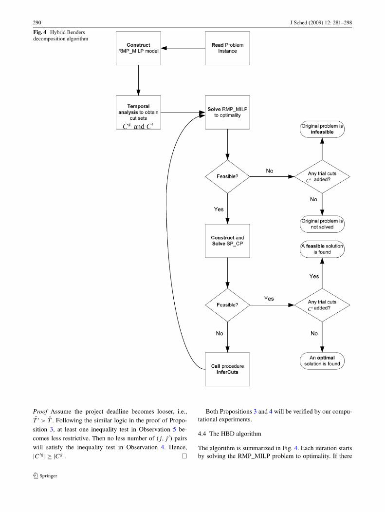
Fig. 4 Hybrid Bendersdecomposition algorithm

Proof Assume the project deadline becomes looser, i.e.,T̄ ′ > T̄ . Following the similar logic in the proof of Propo-sition 3, at least one inequality test in Observation 5 be-comes less restrictive. Then no less number of (j, j ′) pairswill satisfy the inequality test in Observation 4. Hence,|C′g| ≥ |Cg|. �

Both Propositions 3 and 4 will be verified by our compu-tational experiments.

4.4 The HBD algorithm

The algorithm is summarized in Fig. 4. Each iteration startsby solving the RMP_MILP problem to optimality. If there

J Sched (2009) 12: 281–298 291

is no feasible solution found, then the original problem isinfeasible or not solved with the given computational time.Otherwise, the obtained partial solution is used to constructthe feasibility SP_CP problem, which attempts to determineif the partial solution can be extended to a complete solutionthat satisfies the scheduling constraints. If there exists sucha complete solution, then this solution is an optimal solutiongiven that no trial cut has been added into the master prob-lem during the solution process. If the SP_CP is infeasible,the causes of infeasibility are inferred as cuts and added tothe RMP_MILP model through the InferCuts (Procedure 1).The algorithm terminates when the partial solution can beextended to a complete feasible solution, or the RMP_MILPbecomes infeasible.

Assuming that only global cuts from the cut set Cg havebeen added into the RMP_MILP, we state the followingproposition concerning the convergence of our HBD algo-rithm. The proof follows a similar approach as the conver-gence proof in Jain and Grossmann (2001).

Proposition 5 If only global cuts from Cg are added intothe RMP_MILP, the HBD algorithm converges to the op-timal solution or proves infeasibility in a finite number ofiterations.

Proof The assignment subproblem RMP_MILP is eitherfeasible or infeasible as the domain of the decision variablesx and z is bounded. We consider the following two cases.

(i) RMP_MILP is feasible.The domain of RMP_MILP(n) reduces as n increases.

Since the domain of x and z is finite, there exists an iterationξ where the optimal solution (xξ , zξ ) to the master problemleads to a feasible solution t ξ to the scheduling subproblemSP_CP(ξ ). Since global cuts in Cg do not exclude any feasi-ble solution from the original problem according to Propo-sition 1, RMP_MILP(n) is a relaxation of the original prob-lem. Then the solution (xξ , zξ , tξ ) is an optimal solution tothe original problem. Hence, the algorithm will converge toan optimal solution in a finite number of iterations.

(ii) RMP_MILP is infeasible.If the relaxed master problem is infeasible, the subprob-

lem will never obtain a feasible solution. Since the domainof x and z is finite and shrinks with each successive itera-tion, the master problem will become infeasible after a finitenumber of iterations. �

If any trial cut from the set Ct is incurred, Proposition 5will no longer hold due to Proposition 2. Despite this po-tential loss of ability to prove optimality, trial cuts are stillpreferable to the general “no-good” cuts in Jain and Gross-mann (2001). This is because the general “no-good” gener-ated cuts in the context of interrelated personnel are ratherweak, which leads to a slow convergence. Hence, we have

to trade-off the ability to proof optimality with the efficiencyof the algorithm.

Although the proposed decomposition algorithm may notbe able to find optimal solution, it will not remove all fea-sible solutions from the solution space. Note that both theglobal and trial cuts restrict the assignment subproblemrather than scheduling subproblem. The format of trial cuts,preventing a person to be simultaneously assigned to a pairof jobs, serves as a heuristic to resolve the resource conflictscaused by the minimum forbidden sets. Practically speak-ing, it will be costly to examine all possible trial cuts to re-solve resource conflicts, although such an exhaustive searchis able to prove optimality from a theoretical perspective.The computational results, which will be presented next,suggest that our cut-generating scheme is both efficient asof computational time and effective as of solution quality.

Our cut-generating scheme also provides insights on theeffectiveness of the hybrid Benders decomposition. Thelikelihood for the scheduling subproblem to be feasible de-pends largely on the time restrictiveness of the project. Themore time-restrictive the project is, the less flexible is thescheduling subproblem to resolve resource conflicts and themore global cuts to infer (Proposition 3). We state the fol-lowing conjecture.

Conjecture 1 The original problem with a tighter projectdeadline requires more iterations for the HBD algorithm tosolve.

We further expect that the problem with a tighter projectdeadline to be more difficult to prove optimality due to thedifficulty of resolving resource conflicts. That is, trial cutsare more likely to be incurred to resolve infeasibility, eventhough the size of the trial cut set is smaller (Proposition 4).We thus have Conjecture 2.

Conjecture 2 The original problem with a tighter projectdeadline is more difficult for HBD to prove optimality.

Both conjectures will be verified in our computationalstudy presented next.

5 Computational study

A full factorial experimental design is used to conduct thecomputational study. We compare our HBD algorithm withthe pure MILP and CP approach alone, as well as the SLBDalgorithm proposed by Li and Womer (2006b). All the fourapproaches are implemented in ILOG OPL Studio 3.6.1(ILOG 2002c), which uses CPLEX 8.1 (ILOG 2002b) tosolve an MILP, ILOG Solver 5.3 (ILOG 2002a) to solve aCP. The computations are performed on a PC Pentium IV2.4 GHz with 512 Mb RAM.

292 J Sched (2009) 12: 281–298

Table 5 Factors considered inthe experimental design Factor Factor explanation Value

|J| The number of tasks in a project {10, 30}

|K| The number of skills relevant to a project {4, 8}

|S| The personnel availability {Low, High}

RT Restrictiveness of Thesen {0.35, 0.65}

R Multiplier of average number of skills required by a task {0.3, 0.6}

M Multiplier of average number of skills possessed by a person {0.3, 0.6}

DF Deadline factor {Low, High}

5.1 Experimental design

Since our problem and the RCPSP share common dataconcerning the project network, we adopt instances of theRCPSP for our experiments. As our problem also involvesminimal and maximal time lags we choose ProGen/max(Schwindt 1996) to generate the RCPSP instances. Sevencontrol factors in our experiment and their explanations arelisted in Table 5.

The problem size is directly affected by the number oftasks |J|, the number of skills |K|, and personnel availability|S|. In order to have meaningful comparisons, we have con-centrated on the problem space where MILP and CP meth-ods had a chance to remain competitive. In our experiment,|J| is chosen from the two-element set {10, 30} and |K| ischosen from {4, 8}. The low level of personnel availability|S| is chosen such that an instance could be feasible; and thehigh level of |S| is chosen approximately 50% higher thanthe low level of |S|. For example, if it is found that at least60 people are needed for a project, we set the low level of|S| to be 60 and high level to be 60 + 60 ∗ 50% = 90. TheRestrictiveness of Thesen (RT, Thesen 1977) measures thecomplexity of a network and has been shown to have an evengreater effect on the complexity of RCPSP than the numberof tasks |J| (Schwindt 1996). In our experiment, RT is cho-sen from {0.35, 0.65}. The complexity of skill requirementis controlled by the multiplier R representing the averagenumber of skills required by a task, which affects both thescheduling and assignment aspects of the problem. A lowlevel of R is set to be around 0.3 and a high level around0.6. Skill mix complexity is reflected by the multiplier M ofaverage number of skills possessed by an individual, whoseeffect is mainly on the assignment problem. Likewise, a lowlevel of M is set to be around 0.3 and a high level around 0.6.

An important factor we expect to have a significant im-pact on the algorithm performance is the deadline T̄ on theproject makespan. In order to verify Conjectures 1 and 2, wehave set the lower level of T̄ to be lowest possible as longas the problem remains feasible. T̄ is calculated followingDrexl and Kimms (2001):

T̄ = DF · max EFj , (19)

where EFj is the earliest starting time of activity j .

Fig. 5 Number of overlapping activities of a 10-task instance asproject deadline decreases

In order to compare with the SLBD algorithm, we assumethat each person is paid the same salary, so that the objec-tive function reduces to minimizing the number of selectedpersonnel to perform the project.

5.2 Computational results

A running time limit of 10 hours is imposed for all the fourapproaches. For the HBD, a limit of 10 seconds is imposedon the CP scheduling subproblem and 600 seconds on themaster MILP problem. Among the 128 instances, two in-stances are infeasible which leaves a total of 126 feasibleinstances.

5.2.1 The effect of project deadline

We first conducted experiments to analyze the effect ofproject deadline on the number of must-overlapping (‖) andpossible-overlapping (|) activities, i.e., the cardinality of Cg

and Ct . Figure 5 illustrates such an experiment performedon a 10-task instance. As the project becomes more restric-tive (the project deadline represented by DF decreases), thenumber of must-overlapping pairs increases, which supportsProposition 3 and the number of possible-overlapping pairsdecreases, which supports Proposition 4.

Figure 6 illustrates the effect of project deadline on theperformance of HBD on solving the set of 126 instances.

J Sched (2009) 12: 281–298 293

Fig. 6 The effect of project deadline on the performance of HBD

Fig. 7 Comparison of the overall computational results

As we have expected in Conjecture 1, on average theproblem with a loose project deadline can be solved by theHBD algorithm with less effort (fewer cuts). Concerning thealgorithm’s ability to find optimal solutions and prove opti-mality, for the 63 instances with a loose deadline, 57 of them(90%) find optimal solutions and prove optimality (a successrate of 100%); for the other 63 instances with a strict dead-line, 49 of them (77%) find optimal solutions and only 45 ofthe 49 optimal solutions have been proved to be optimal witha success rate of 92%. These results support Conjecture 2.

5.2.2 Comparison of algorithm performance

We now compare the overall performance of the four ap-proaches.

As we can see from Fig. 7, only the two decompositionalgorithms HBD and SLBD have found feasible solutionsto all of the 126 problems. The HBD is able to find moreoptimal solutions than any of the other approaches. HBD isadvantageous over the heuristic approach SLBD since thereis no way for SLBD to prove optimality. Notably, HBD hasan overall success rate of 96% to prove optimality (when anoptimal solution is found) in contrast to 83% of MILP.

We further compare solution quality as shown in Fig. 8.Clearly, the HBD outperforms the other three in objective

function value, saving about one person over MILP and twopersons over CP for each problem instance on average. The

Fig. 8 Comparison of the sum of objective values

Fig. 9 Comparison of the average project makespan

SLBD is the second best among the four with better solutionquality than the pure MILP or CP approach alone.

Although project makespan does not appear in the ob-jective function, desirably one prefers the schedule witha shorter makespan when it results in the same objec-tive value as other solutions. Interestingly, the four ap-proaches produce different project makespan in their bestsolutions found. The HBD provides solutions with the short-est makespan on average as indicated by Fig. 9. It excelsby an average of 4 time units over CP, 11 time units overSLBD, and almost 14 time units over MILP. These couldrepresent tremendous time savings on scheduling a projectin the real world: the HBD finds schedules not only with lesscost but also with shorter makespan. This merit of HBD canbe attributed to its decomposition characteristic. The HBDdecomposes the original problem into a pure GAP and apure single-mode RCPSP, where the project makespan canbe well handled by CP techniques. This also explains thefact that the pure CP approach is the second best in the qual-ity of makespan. In contrast with HBD, the SLBD is do-ing the opposite by finding a feasible schedule first and thensolving the assignment part. It always starts from the mostrestrictive skill level (lowest possible resource availability),which potentially leads to a longer makespan. From a differ-ent perspective, the SLBD can be viewed as a time-resourcetrade-off approach. Since the SLBD is greedy toward find-ing solutions with lower costs, the quality of makespan has

294 J Sched (2009) 12: 281–298

Table 6 Regression resultswith objective value asdependent variable

*This estimate is significantlydifferent from zero at 95%confidence level

CP HBD SLBD MILP

Intercept −40.864 −31.500 −31.448 −43.733

|J| 1.024* 1.024* 1.012* 1.110*

|K| 3.575* 2.900* 2.933* 3.331*

|S| 2.324 1.086 1.268 2.551

RT −8.087 −9.921* −10.150* −7.955

R 14.864* 12.758* 12.857* 14.480*

M 0.512 −0.258 −0.358 1.332

DF −0.381 −0.365 −0.333 0.0635

Adjusted R-square 0.778 0.800 0.801 0.701

Fig. 10 Comparison of the average computational time

to be sacrificed to some degree. The pure MILP approachperforms the worst among the four in project makespan. Dif-ferent from the decomposition approach, the MILP attemptsto solve the original problem with a mixture of assignmentand scheduling variables and constraints, which does not ex-ploit the structure of the problem at all. Thus, it often fails tofind a shorter makespan for a given assignment when thereexists such a makespan.

Next we compare the average computational time foreach approach to find their best solutions in Fig. 10.

The two decomposition algorithms are significantlyfaster than the pure MILP and CP algorithms alone. TheSLBD is the fastest among the four due to its heuristic na-ture, spending considerably less running time than the otherthree, i.e., around 1/11 of HBD, 1/45 of MILP, and 1/72of CP. HBD is the second best with about 1/4 of the run-ning time of MILP and 1/7 of CP. The efficiency of CPfor solving scheduling problems has been greatly hamperedby the assignment part of PSMPR. With decomposition, theadvantage of CP has been fully exploited, solving a feasi-bility scheduling subproblem within seconds and saving theoverall computational time significantly.

5.2.3 Multi-factor analysis

Multiple linear regression (MLR) is used to quantify the ef-fects of the factors on the algorithm performance. We find

that both the objective value and makespan can be well ex-plained by MLR. The computational time, however, cannotbe well explained with an R-square less than 30%. This isprobably due to the problem’s combinatorial nature and NP-hardness such that even a small-size instance may take along time to solve. Table 6 shows the regression results withobjective value as dependent variable.

It is clear that the decomposition algorithms HBD andSLBD have higher adjusted R-square than the direct ap-proaches, which is probably because they are structured tohandle different types of subproblems separately instead ofsolving the original problem directly. Also notice that thenetwork complexity represented by RT is significantly non-zero only for the two decomposition approaches.

The regression results for the makespan as dependentvariable are presented in Table 7. Instead of using RT di-rectly, we have used |J| ∗ RT to capture the interactive ef-fect between |J| and RT, which improves the adjusted R-square from around 70% to over 90% for the decompositionapproaches. Again, HBD and SLBD have higher adjustedR-square.

The regression equations obtained above can be used toconstruct the three-dimensional surface graphs for compar-ing algorithm performance. This analysis provides us witha visualization of which algorithm dominates the other inwhat regions of the problem space. We set the differenceof the performance measures (objective value or makespan)between two methods as a dependent variable and vary thenumber of tasks |J| and the number of skills |K|, which aretwo major factors affecting the problem size and are bothsignificant in the associated regression functions.

Figure 11 through Fig. 13 compares HBD with MILP,CP and SLBD in objective function value, respectively. Fig-ure 11 shows that the HBD tends to dominate MILP in ob-jective value when |J| or |K| increases. From Fig. 12 we ob-serve that although |J| does not seem to have much impacton the difference of objective value between HBD and CP,as |K| increases the advantage of HBD over CP increases.Figure 13 indicates that when |J| increases, the SLBD tends

J Sched (2009) 12: 281–298 295

Table 7 Regression resultswith makespan as dependentvariable

*This estimate is significantlydifferent from zero at 95%confidence level

CP HBD SLBD MILP

Intercept −72.871 −47.850 −84.194 −147.090

|J| 1.609* 1.482* 2.450* 3.077*

|K| 6.955* 4.982* 3.400* 6.468*

|S| −5.820 −0.366 −1.442 11.00290

R 9.257 0.960 8.723* 17.153*

M −2.664 0.228 −0.00460 −0.966

DF 9.683 1.667 22.492* 29.381*

J ∗ RT 7.869* 7.571* 7.182* 6.765*

Adjusted R-square 0.809 0.919 0.904 0.725

Fig. 11 HBD dominates MILP below zero for objective value

Fig. 12 HBD dominates CP below zero for objective value

to dominate HBD, which is not surprising given the heuris-tic nature of SLBD and the computational time limits im-posed on the HBD. However, as |K| increases the advantageof HBD over SLBD increases.

Fig. 13 HBD dominates SLBD below zero for objective value

Fig. 14 HBD dominates MILP below zero for makespan

Figure 14 through Fig. 16 compares HBD with MILP, CPand SLBD in project makespan, respectively. We observefrom Figs. 14 and 15 that the HBD tends to dominate bothMILP and CP in project makespan when |J| or |K| increases.Figure 16 shows that the only problem space in which the

296 J Sched (2009) 12: 281–298

Fig. 15 HBD dominates CP below zero for makespan

SLBD dominates HBD is where |J| is small and |K| is large(e.g., |J| = 5 and |K| = 8), which does not seem likely tooccur in real world problems.

6 Discussions

Although we present our model and hybrid decomposi-tion algorithm in the context of a pure scheduling prob-lem, our modeling and solution approach can be modi-fied to cope with various planning problems. A variantof our model has been applied to the US Navy’s DDXcrew optimization problem (Li and Womer 2006a), whichfinds the minimum number of sailors with optimal skillmix to man a ship, while completing a specific missionconsisting of interrelated tasks. There, the resource as-signment subproblem is modeled as a bin packing prob-lem with conflicts (BPC, Jasen 1999); while the result-ing scheduling subproblem leads to a single-mode RCPSPwith unary resources. This application aids the decisionmaker to plan for necessary training requirements in theintermediate run. A closely related model, the multi-modeRCPSP as discussed in Sect. 2.3, has been applied to tacklean important planning problem in the supply chain op-timization field, namely, the supply chain configurationproblem with explicit resource and capacity constraints (Liand Womer 2008). There, the assignment aspect involveschoosing the optimal configurations/modes for each activ-ity/process in the supply chain (discrete decision domain);while the scheduling aspect involves determining the in-bound and outbound service times of each process subjectto temporal constraints (continuous decision domain).

We now examine the relationship between our proposedmodel/algorithm and the temporal planning problems inthe planning research community, which involve arrang-ing actions and assigning resources in order to accomplishgiven tasks and objectives over a period of time (Fox and

Fig. 16 HBD dominates SLBD below zero for makespan

Long 2003; Wah and Chen 2006). Note that both schedul-ing and assignment decisions are critical in the temporalplanning problem: (i) on one hand, time-related technicalrequirements are often modeled by a network of temporalconstraints (Dechter et al. 1991); (ii) on the other hand,the execution of activities requires renewable resources—machines, vehicles, or skilled personnel (as consideredin this paper), which often gives rise to resource allo-cation/assignment type of subproblems resembling multi-processor scheduling or bin packing problems (Fox andLong 2001). Both (i) and (ii) fit well into our modelingframework. To be specific, the work-break-down structure(WBS) in project scheduling makes it flexible in defining ac-tivities with different levels of details. Moreover, the gener-alized temporal constraints considered in our model capturea rich set of time dependencies, such as overlaps and delaysin addition to precedence relations (Neumann et al. 2002),which are ubiquitous in the planning context (Dechter et al.1991). As for the resource allocation decisions, the inclusionof workloads of renewable resource units makes it possibleto allocate each resource unit through the planning horizon.It is also possible to allow the resource availability vary overtime.

Our hybrid decomposition algorithm also shares somesimilar insights with certain solution approaches developedin the temporal planning field. Notably, Fox and Long(2001) present domain analysis techniques to identify andextract subproblems, for which effective and efficient solu-tion methods are available. They also stress the challengeof integrating different solution procedures to cooperate insolving the original problem. In our HBD algorithm, theoriginal problem is decomposed into an assignment sub-problem and a scheduling subproblem, which is solved byinteger programming methods and constraint programming,respectively. The two solvers are linked together via “cuts”generated by temporal analysis. Such an OR/AI hybridframework was recently advocated by Fox (2006), and wasbelieved to be an promising line of research in the planning

J Sched (2009) 12: 281–298 297

community. Another study of utilizing such a hybrid strat-egy, that integrates max-SAT technique in AI and programevaluation and review technique (PERT) in OR, to cope withtemporal planning is provided by Xing et al. (2006). Thesolution approach by Wah and Chen (2006) relies on con-straint partitioning, which decomposes the original probleminto significantly smaller subproblems. Instead of generating“cuts” to resolve violations of global constraints, they devisea penalty formulation and adjust the weights of violated con-straints to resolve conflicts. The HBD paradigm also sharessome similarities with the so called Squeaky Wheel Opti-mization (SWO) proposed by Joslin and Clements (1999).The core of SWO is a Construct/Analyze/Prioritize cycle.The Construct component operates in the solution space,which is analogous to solving the relaxed master problemin HBD. The Prioritize component operates in the prioriti-zation space to iteratively generate new priorities for Con-struct. The Analyze component serves as the link betweenConstruct and Prioritize, which finds “troubled” elementsin the current solution. The role of Analyze is much simi-lar to that of the cut generating scheme in our HBD, whichdeduces “violated” assignment constraints and adds them it-eratively to the master problem. Frank and Kurklu (2005)successfully applied SWO to an optimization problem thatlies on the scheduling boundaries of classical planning onSOFIA at NASA.

7 Conclusions and future research

In this paper, we studied the project scheduling problemwith multi-skilled personnel to minimize the total staffingcosts for executing a project. Our model is general enoughto include minimum and maximum time lags as general-izations to precedence constraints in traditional machinescheduling settings. The model also takes each individual’sworkload capacity into consideration, a feature often neededin realistic personnel scheduling. We also show the rele-vance of our model to the planning research community, inparticular, the temporal planning problems.

We developed a hybrid MILP/CP Benders decomposi-tion (HBD) algorithm to solve this strongly NP-hard prob-lem. The key to the practical effectiveness and efficiencyof our algorithm is the use of temporal analysis to generateproblem-specific cuts (instead of the general no-good cuts)during the Benders decomposition iterations. The computa-tional results show that the HBD excels other approachesin solution quality with reasonable computational time. No-tably, the HBD finds and proves more optimal solutions thanthe pure MILP method while spending significantly lesscomputation time. When the project does not have a restric-tive deadline, it performs particularly well (with a success

rate of 100% to prove optimality for the set of tested prob-lem instances). The solution quality of HBD is also robustas evident by our multi-factor analysis.

Two lines of research could be conducted in the future.From a modeling perspective, it might be interesting to con-sider personnel’s skill proficiency. This can be achieved byeither generalizing the objective function to minimize thetotal assignment costs or let task/skill’s processing time de-pend on assigned personnel’s proficiency level. From an al-gorithmic perspective, alternative hybrid strategies could beapplied within the HBD framework proposed in this pa-per. This is motivated by the fact that it is still costly forMILP methods to solve the relaxed master problem whichis NP-hard itself. Inspired by the branch–and–check ap-proach of Thorsteinsson (2001) where the master problemdoes not need to be solved to optimality, we could applya local search heuristic to obtain a good quality solution tothe master problem, which leads to a hybrid local search andconstraint programming algorithm. This development is par-ticularly attractive when dealing with large size problems inthe real world. It will also be interesting to further explorethe possibility for the HBD paradigm to cope with the tem-poral planning problems in the planning research commu-nity, given the analogies between the optimization problemstudied in this paper and temporal planning problem.

Acknowledgements This research was supported by the Office ofNaval Research (ONR) under Grant No. N00140310621. We wouldalso like to thank Derek Long and two anonymous referees for theirdetailed and constructive comments that help improve this paper.

References

Aksin, O. Z., Karaesmen, F., & Ormeci, E. L. (2006). A review ofworkforce cross-training in call centers from an operations man-agement perspective. In D. Nembhard (Ed.), Workforce crosstraining handbook. Boca Raton: CRC Press.

Baptiste, P., Le Pape, C., & Nuijten, W. (2001). Constraint-basedscheduling: applying constraint programming to scheduling prob-lems. New York: Springer.

Bartusch, M., Mohring, R. H., & Randermacher, F. J. (1988). Schedul-ing project networks with resource constraints and time windows.Annals of Operations Research, 16, 201–240.

Bellenguez, O., & Neron, E. (2004). Methods for solving the multi-skill project scheduling problem. In Proceedings of the ninth in-ternational workshop on project management and scheduling,Nancy, France.

Benders, J. F. (1962). Partition procedures for solving mixed variablesprogramming problems. Numerische Mathematik, 4, 238–252.

Benoist, T., Laburthe, F., & Rotternbourg, B. (2001). Lagrange re-laxation and constraint programming collaborative schemes fortraveling tournament problems. In Integration of AI and OR tech-niques in constraint.

Benoist, T., Gaudin, E., & Rotternbourg, B. (2002). Constraint pro-gramming contribution to Benders decomposition: A case study.In The eighth international conference on principles and practiceof constraint programming, Ithaca, New York.

298 J Sched (2009) 12: 281–298

Bockmayr, A., & Kasper, T. (1998). A unifying framework for integerand finite domain constraint programming. INFORMS Journal onComputing, 10(3), 287–300.

Brucker, P. (2001). Scheduling algorithms. Berlin: Springer.Brucker, P. (2002). Scheduling and constraint propagation. Discrete

Applied Mathematicsu, 123(1–3), 227–256.Brucker, P., & Knust, S. (1998). Solving large-sized resource-

constrained project scheduling problems. In J. Weglarz (Ed.),Project scheduling: recent models, algorithms and applications.Dordrecht: Kluwer Academic.

Brucker, P., & Knust, S. (2000). A linear programming and constraintpropagation-based lower bound for the RCPSP. European Journalof Operational Research, 127(2), 335–362.

Brucker, P., & Knust, S. (2003). Lower bounds for resource-constrained project scheduling problems. European Journal ofOperational Research, 149, 302–313.

Brucker, P., Drexl, A., Mohring, R. H., Neumann, K., & Pesch, E.(1999). Resource-constrained project scheduling: Notation, clas-sification, models and methods. European Journal of OperationalResearch, 112(1), 3–41.

Dechter, R., Meiri, I., & Pearl, J. (1991). Temporal constraint networks.Artificial Intelligence, 49(1–3), 61–95.

Dincbas, M., Van Hentenryck, P., Simonis, H., & Aggoun, A. (1988).The constraint logic programming language CHIP. In Proceedingsof the 2nd international conference on fifth generation computersystems.

Drexl, A., & Kimms, A. (2001). Optimization guided lower and upperbounds for the resource investment problem. Journal of Opera-tional Research Society, 52, 340–351.

Drexl, A., Juretzka, J., Salewski, F., & Schirmer, A. (1998). New mod-eling concepts and their impact on resource-constrained projectscheduling. In J. Weglarz (Ed.), Project scheduling: recent mod-els, algorithms and applications. Dordrecht: Kluwer Academic.

Easton, K., Nemhauser, G., & Trick, M. (2004). CP based branch–and–price. In M. Milano (Ed.), Constraint and integer programming.Berlin: Springer.

Eremin, A., & Wallace, M. (2001). Hybrid Benders decomposition al-gorithms in constraint logic programming. Lecture Notes in Com-puter Science, 2239, 1–15.

Focacci, F., Laborie, P., & Nuijten, W. (2000). Solving schedulingproblems with setup times and alternative resources. In Proceed-ings of the fifth international conference on artificial intelligenceplanning and scheduling.

Fox, M. (2006). Planning for mixed discrete continuous domains. InJ. C. Beck & B. M. Smith (Eds.), Lecture notes in computer sci-ence: Vol. 3990. CPAIOR 2006 (p. 2). Berlin: Springer.

Fox, M., & Long, D. (2001). Hybrid STAN: Identifying and manag-ing combinatorial optimization sub-problems in planning. In Pro-ceedings of the international joint conference on artificial intelli-gence (IJCAI).

Fox, M., & Long, D. (2003). PDDL2.1: An extension to PDDL forexpression temporal planning domains. Journal of Artificial Intel-ligence Research, 20, 61–124.

Frank, J., & Kurklu, E. (2005). Mixed discrete and continuous al-gorithms for scheduling airborne astronomy observations. InR. Batak & M. Milano (Eds.), Lecture notes in computer science:Vol. 3524. CPAIOR 2005 (pp. 183–200). Berlin: Springer.

Harvey, W., & Ginsberg, M. (1995). Limited discrepancy search. InThe fourteenth international joint conference on artificial intelli-gence (IJCAI-95).

Hooker, J. (2000). Logic-based methods for optimization: combin-ing optimization and constraint satisfaction. New York: Wiley-Interscience.

Hooker, J. (2002). Logic, optimization and constraint programming.INFORMS Journal on Computing, 14(4), 285–321.

Hooker, J., & Osorio, M. (1999). Mixed logical-linear programming.Discrete Applied Mathematics, 96–97, 395–442.

ILOG (2002a). ILOG Solver 5.3 User’s Manual.ILOG (2002b). ILOG CPLEX 8.1 User’s Manual.ILOG (2002c). OPL Studio 3.6.1 User’s Manual: ILOG, Inc.Jain, V., & Grossmann, I. (2001). Algorithms for hybrid MILP/CP

models for a class of optimization problems. INFORMS Journalon Computing, 13(4), 258–276.

Jasen, K. (1999). An approximation scheme for bin packing with con-flicts. Journal of Combinatorial Optimization, 3, 363–377.

Joslin, D. E., & Clements, D. P. (1999). “Squeaky Wheel” optimiza-tion. Journal of Artificial Intelligence Research, 10, 353–373.

Lasdon, L. S. (1970). Optimization theory for large systems. New York:Macmillan Co.

Li, H., & Womer, K. (2006a). Determining crew composition for a newtechnology (Working Paper).

Li, H., & Womer, K. (2006b). Project scheduling with multi-purposeresources: a combined MILP/CP decomposition approach. Inter-national Journal of Operations and Quantitative Management,12(4), 305–325.

Li, H., & Womer, K. (2008). Modeling the supply chain configura-tion problem under resource constraints. International Journal ofProject Management, 26(6), 646–654.

Milano, M., & Trick, M. (2004). Constraint and integer programming.In M. Milano (Ed.), Constraint and integer programming: towarda unified methodology. Berlin: Springer.

Nemhauser, G., & Wolsey, L. (1988). Integer and combinatorial opti-mization. New York: Wiley.

Neron, E., Bellenguez, O., & Heurtebise, M. (2006). Decompositionmethod for solving multi-skill project scheduling problem. In Pro-ceedings of the tenth international workshop on project manage-ment and scheduling, Poznan.

Neumann, K., Schwindt, C., & Zimmermann, J. (2002). Projectscheduling with time windows and scarce resources: temporal andresource-constrained project scheduling with regular and nonreg-ular objective functions. New York: Springer.

Schwindt, C. (1996). Generation of resource-constrained projectscheduling problems with minimal and maximal time lags (Tech-nical Report WIOR-489). Institute für Wirtschaftstheorie und Op-erations Research, University of Karlsruhe.

Sellmann, M., & Fahle, T. (2003). Constraint programming based La-grangian relaxation for the automatic recording problem. Annalsof Operations Research, 118, 17–33.

Thesen, A. (1977). Measures of the restrictiveness of project networks.Networks, 7, 193–208.

Thorsteinsson, E. S. (2001). Branch–and–check: A hybrid frameworkintegrating mixed integer programming and constraint logic pro-gramming. In Proceedings of the seventh international conferenceon principles and practices of constraint programming (CP-01).Berlin: Springer.

Tsang, E. (1993). Foundations of constraint satisfaction. San Diego:Academic Press.

Van Hentenryck, P. (1999). The OPL optimization programming lan-guage. Cambridge: MIT Press.

Wah, B. W., & Chen, Y. (2006). Constraint partitioning in penalty for-mulations for solving temporal planning problems. Artificial In-telligence, 170, 187–231.

Wallace, M., Novello, S., & Schimpf, J. (1997). ECLiPSe:A platform for constraint logic programming. Available from:http://www.icparc.ic.ac.uk/eclipse/reports/eclipse/eclipse.html.

Xing, Z., Chen, Y., & Zhang, W. (2006). An efficient hybrid strategy fortemporal planning. In J. C. Beck & B. M. Smith (Eds.), Lecturenotes in computer science: Vol. 3990. CPAIOR 2006 (pp. 273–287). Berlin: Springer.