Scheduling and Resource Allocation in OFDMAWireless Systems

Jianwei Huang, Vijay Subramanian, Randall Berry, and Rajeev Agrawal

February 2009

Book chapter in “Orthogonal Frequency Division Multiple Access Fundamentalsand Applications.”

1 Introduction

Scheduling and resource allocation are essential components of wireless data systems.Here by scheduling we refer the problem of determining which users will be activein a given time-slot; resource allocation refers to the problem of allocating physical-layer resources such as bandwidth and power among these active users. In modernwireless data systems, frequent channel quality feedback is available enabling boththe scheduled users and the allocation of physical layer resources to be dynamicallyadapted based on the users’ channel conditions and quality of service (QoS) require-ments. This has led to a great deal of interest both in practice and in the researchcommunity on various “channel aware” scheduling and resource allocation algorithms.Many of these algorithms can be viewed as “gradient-based” algorithms, which selectthe transmission rate vector that maximizes the projection onto the gradient of thesystem’s total utility [1–4, 8, 9, 25, 28, 29]. One example is the “proportionally fairrule” [3,4] first proposed for CDMA 1xEVDO based on a logarithmic utility functionof each user’s throughput. A larger class of throughput-based utilities is consideredin [2] where efficiency and fairness are allowed to be traded-off. The “Max Weight”policy (e.g. [6–8]) can also be viewed as a gradient-based policy, where the utility isnow a function of a user’s queue-size or delay.

Compared to TDMA and CDMA technologies, OFDMA divides the wireless re-source into non-overlapping frequency-time chunks and offers more flexibility for re-source allocation. It has many advantages such as robustness against intersymbol

1

interference and multipath fading as well as and lower complexity of receiver equal-ization. Owing to these OFDMA has been adopted the core technology for most recentbroadband wireless data systems, such as IEEE 802.16 (WiMAX), IEEE 802.11a/g(Wireless LANs), and LTE for 3GPP.

This chapter discusses gradient-based scheduling and resource allocation in OFDMAsystems. This builds on previous work specific to the single cell downlink [28] anduplink [25] setting (e.g., Fig. 1). The key contribution of the book chapter is provid-ing a general framework that includes each of these as special cases and also appliesto multiple cell/sector downlink transmissions (e.g., Fig. 2). In particular, severalimportant practical constraints are included in this framework, namely, 1) integerconstraints on the tone allocation, i.e., a tone can be allocated to at most one user; 2)constraints on the maximum SNR (i.e., rate) per tone, which models a limitation onthe available modulation and coding schemes; 3) “self-noise” on tones due to channelestimation errors (e.g., [11]) or phase noise [24]; and 4) user-specific minimum andmaximum rate constraints. We not only provide the optimal algorithm for solvingthe optimization problem corresponding to the generalized model, but also providelow complexity heuristic algorithms that achieve close to optimal performance.

Most previous work on OFDMA systems focused on solving the resource allocationproblem without jointly considering the problem of user scheduling. We will brieflysurvey this work in the next section. Then we describe our general formulationtogether with the optimal and heuristic algorithms to solve the problem. Finally, wewill summarize the chapter and outline some future research directions.

Base Station

User 1

User 2

User K

Base Station

User 1

User 2

User K

Single Cell Downlink Communications Single Cell Uplink Communications

Figure 1: Example of a single cell downlink (left) and uplink scenerio (right).

2

Base Station 1

User 1

User 2

User K1

Base Station 2

User 1

User 2

User K2

Base Station 3

User 1

User 2

User K3

Figure 2: Example of a multiple cell/sector downlink scenerio (the different basestations could represent different sectors of the same base station shown by the circle).

3

2 Related Work on OFDMA resource allocation

A number of formulations for single cell downlink OFDMA resource allocation havebeen studied (e.g., [12–21]). In [13, 14], the goal is to minimize the total transmitpower given target bit-rates for each user. In [14], the target bit-rates are determinedby a fair queueing algorithm, which does not take into account the users’ channelconditions. A number of papers including [15–18, 20, 21] have studied various sum-rate maximization problems, given a total power constraint. In [16–18] there is also aminimum bit-rate per user that must be met. [21] considers both minimum and max-imum rate targets for each user and also takes into account several constraints thatarise in Mobile WiMax. In [20], certain “delay sensitive” users are modeled as havingfixed target bit-rate (i.e. their maximum and minimum rates are the same), whileother “best effort” users have no bit-rate constraints. Thus the scheduler attempts tomaximize the sum-rate of the best effort users while meeting the rate-targets of thedelay sensitive ones. In [12,19], weighted sum-rate maximization is considered. Thisis a special case of the resource allocation problem we study here for a given time-slot but does not account for constraints on the SNR per carrier, rate constraints, orself-noise. In [12], a suboptimal algorithm with constant power per tone was shownin simulations to have little performance loss. Other heuristics that use a constantpower per tone are given in [15–17]; we will briefly discuss a related approach in Sec-tion 4. In [19], a dual-based algorithm similar to ours is considered, and simulationsare given which show that the duality gap of this problem quickly goes to zero asthe number of tones increases. In [22], the information theoretic capacity region of asingle cell downlink broadcast channel with frequency-selective fading using a TDMscheme is given; the feasible rate region we consider, without any maximum SNRand rate constraints, can be viewed as a special case of this region. None of thesepapers consider self-noise, rate constraints or per user SNR constraints. Moreover,most of these papers optimize a static objective function, while we are interested in adynamic setting where the objective changes over time according to a gradient-basedalgorithm. It is not a priori clear if a good heuristic for a static problem appliedto each time-step will be a good heuristic for the dynamic case, since the optimalityresult in [1–3,6–8,29] is predicated on solving the weighted-rate optimization problemexactly in each time-slot. Simulation results in [28] show that this does hold for theheuristics presented in Section 4.

Resource allocation for a single cell OFDMA uplink has been presented in [32–39].In [32], a resource allocation problem was formulated in the framework of Nash Bar-gaining, and an iterative algorithm was proposed with relatively high complexity.The authors of [33] proposed a heuristic algorithm that tries to minimize each user’stransmission power while satisfying the individual rate constraints. In [34], the authorconsidered the sum-rate maximization problem, which is a special case of the problem

4

considered here with equal weights. The algorithm derived in [34] assumes Rayleighfading on each subchannel; we do not make such an assumption here. In [35], an up-link problem with multiple antennas at the base station was considered; this enablesspatial multiplexing of subchannels among multiple users. Here, we focus on singleantenna systems where at most one user can be assigned per sub-channel. The workin [36–39] is closer to our model. The authors in [36] also considered a weighted ratemaximization problem in the uplink case, but assumed static weights. They proposedtwo algorithms, which are similar to one of the algorithms described in this chapter.We propose several other algorithms that outperform those in [36] with similar orslightly higher complexity. Paper [37] generalized the results in [36] by consideringutility maximization in one time-slot, where the utility is a function of the instan-taneous rate in each time-slot. Another work that focused on per time-slot fairnessis [39]. Finally, [38] proposed a heuristic algorithm based on Lagrangian relaxation,which has high complexity due to a subgradient search of the dual variables.

Resource allocation and interference management of multi-cell downlink OFDMAsystems were presented in [42–49]. A key focus of these works is on interferencemanagement among multiple cells. Our general formulation includes the case whereresource coordination leads to no interference among different cells/sectors/sites. Inour model, this is achieved by dynamically partitioning the subchannels across thedifferent cells/sectors/sites. In addition to being easier to implement, the interfer-ence free operation assumed in our model allows us to optimize over a large class ofachievable rate regions for this problem. If the interference strength is of the orderof the signal strength, as would be typical in the broadband wireless setting, thenthis partitioning approach could also be the better option in an information theoreticsense [31].1

3 OFDMA Scheduling and Resource Allocation

3.1 Gradient-based Wireless Scheduling and Resource Allo-cation Problem Formulation

Let us consider a network with a total of K users. In each time-slot t, the schedul-ing and resource allocation decision can be viewed as selecting a rate vector rt =(r1,t, . . . , rK,t) from the current feasible rate region R(et) ⊆ RK

+ . If a user is notscheduled his rate is simply zero. Here et indicates the time-varying channel state

1We note that our discussions do not directly apply to the case of frequency reuse, where differentnon-adjacent cells may use the same frequency bands. In practice, frequency reuse is typicallyconsidered together with fixed frequency allocations, while here we consider dynamic frequencyallocations across different cells.

5

information of all users available at the scheduler at time t. The decision on therate vector is made according to the gradient-based scheduling framework in [1–3,29]that is basically a stochastic version of the conditional gradient/Frank-Wolfe algo-rithm [26]. Namely, an rt ∈ R(et) is selected that has the maximum projection ontothe gradient of the system’s total utility function

U(Wt) :=K∑i=1

Ui(Wi,t), (1)

where Ui(·) is an increasing concave utility function that measures user i’s satisfactionfor different values of throughput, and Wi,t is user i’s average throughput up to timet. In other words, the scheduling and resource allocation decision is the solution to

maxrt∈R(et)

∇U(Wt)T · rt = max

rt∈R(et)

K∑i=1

U ′i(Wi,t)ri,t, (2)

where U ′i(·) is the derivative of Ui(·). As a concrete example, it is useful to considerthe class of commonly used iso-elastic utility functions given in [2, 5],

Ui(Wi,t) =

{ciα

(Wi,t)α, α ≤ 1, α 6= 0,

ci log(Wi,t), α = 0,(3)

where α ≤ 1 is a fairness parameter and ci is a QoS weight. In this case, after takingderivatives, (2) becomes

maxrt∈R(et)

∑i

ci(Wi,t)α−1ri,t. (4)

With equal class weights (ci = c for all i), setting α = 1 results in a scheduling rulethat maximizes the total throughput during each slot. For α = 0, this results in theproportionally fair rule, and as α increases without bound, we get closer to a max-minfair solution. Thus, this family of utility functions yields a flexible class of policies:the α parameter allows for the choice of an appropriate fairness objective while theci parameter allows one to distinguish relative priorities within each fairness class.

However, more generally, we consider the problem of

maxrt∈R(et)

∑i

wi,tri,t, (5)

where wi,t ≥ 0 is a time-varying weight assigned to the ith user at time t. In the caseof (4), we let wi,t = ci(Wi,t)

α−1. In (4) these weights are given by the gradients ofthroughput-based utilities; however, other methods for generating the weights (pos-sibly depending upon queue-lengths and/or delays [6–8]) are also possible. We note

6

that (5) must be re-solved at each scheduling instance because of changes in both thechannel state and the weights (e.g., the gradients of the utilities). While the formerchanges are due to the time-varying nature of wireless channels, the latter changesare due to new arrivals and past service decisions.

3.2 General OFDMA rate regions

The solution to (5) depends on the channel state dependent rate region R(e), wherewe suppress the dependence on time for simplicity. We consider a model appropriatefor general OFDMA systems including single cell downlink and uplink as well asmultiple cell/sector/site downlink with frequency sharing; related single cell downlinkand uplink models have been considered in [12, 22, 25, 28]. In this model, R(e) isparameterized by the allocation of tones to users and the allocation of power acrosstones. In a traditional OFDMA system at most one user may be assigned to anytone. Initially, as in [13,14], we make the simplifying assumption that multiple userscan share one tone using some orthogonalization technique (e.g. TDM).2 In practice,if a scheduling interval contains multiple OFDMA symbols, we can implement suchsharing by giving a fraction of the symbols to each user; of course, each user will beconstrained to use an integer number of symbols. Also, with a large number of tones,adjacent tones will have nearly identical gains, in which case this time-sharing canalso be approximated by frequency sharing. The two approximations becomes tightas the number of symbols or tones increases, respectively. We discuss the case whereonly one user can use a tone in Section 4.

Let N = {1, . . . , N} denote the set of tones3 and K = {1, 2, . . . , K} the set ofusers. For each j ∈ N and user i ∈ K, let eij be the received signal-to-noise ratio(SNR) per unit transmit power. We denote the transmit power allocated to user i ontone j by pij, and the fraction of that tone allocated to user i by xij. As tones areshared resources, the total allocation for each tone j must satisfy

∑i xij ≤ 1. For a

given allocation, with perfect channel estimation, user i’s feasible rate on tone j is

rij = xijB log

(1 +

pijeijxij

),

which corresponds to the Shannon capacity of a Gaussian noise channel with band-width xijB and received SNR pijeij/xij.

4 This SNR arises from viewing pij as the

2We focus on systems that do not use superposition coding and successive interference cancellationwithin a tone, as such techniques are generally considered too complex for practical systems.

3In practice, tones may be grouped into subchannels and allocated at the granularity of sub-channels. As discussed in [28], our model can be applied to such settings as well by appropriatelyredefining the sub-channel gains {eij} and interpreting N as the set of sub-channels.

4To better model the achievable rates in a practical system we can re-normalize eij by γeij , where

7

energy per time-slot user i uses on tone j; the corresponding transmission power be-comes pij/xij when only a fraction xij of the tone bandwidth is allocated. Similarlythis can also be explained by time-sharing as follows: a channel of bandwidth B isused only a fraction xij of the time with average power pij which leads to the powerduring channel usage to be pij/xij. Without loss of generality we set B = 1 in thefollowing.

3.2.1 Self-noise

In a realistic OFDMA system, imperfect carrier synchronization and channel esti-mation may result in “self-noise” (e.g. [11, 24]). We follow a similar approach asin [11] to model self-noise. Let the received signal on the jth tone of user i be givenby yij = hijsij + nij, where hij, sij and nij are the (complex) channel gain, trans-mitted signal and additive noise, respectively, with nij ∼ CN (0, σ2).5 Assume thathij = hij + hij,δ, where hij is receiver i’s estimate of hij and hij,δ ∼ CN (0, δ2

ij). After

matched-filtering, the received signal will be zij = h∗ijyij resulting in an effective SNRof

Eff-SNR =‖hij‖4pij

σ2ij‖hij‖2 + δ2

ijpij‖hij‖2=

pijeij1 + βijpijeij

, (6)

where pij = E(‖sij‖2), βij =δ2ij

‖hij‖2and eij =

‖hij‖2σ2ij.6 Here, βijpijeij is the self-noise

term. As in the case without self-noise (βij = 0), the effective SNR is still increasingin pij. However, it now has a maximum of 1/βij.

In general, βij may depend on the channel quality eij. For example, this happenswhen self-noise arises primarily from estimation errors. The exact dependence willdepend on the details of channel estimation. As an example, using the model in [23,Section IV] it can be shown that when the pilot power is either constant or inverselyproportional to channel quality subject to maximum and minimum power constraints(modeling power control), β is inversely proportional to the channel condition forlarge e. On the other hand βij = β is a constant when self-noise is due to phase noiseas in [24]. For simplicity of presentation, we assume constant βij = β in the remainderof the paper (except in Fig. 4 where we we allow β(e) ∝ 1/e to illustrate the impact

γ ∈ [0, 1] represents the system’s “gap” from capacity.5We use the notation x ∼ CN (0, b) to denote that x is a 0 mean, complex, circularly-symmetric

Gaussian random variable with variance b := E(‖x‖2).6This is slightly different from the Eff-SNR in [11] in which the signal power is instead given by

‖hij‖4pij ; the following analysis works for such a model as well by a simple change of variables. Forthe problem at hand, (6) seems more reasonable in that the resource allocation will depend only onhij and not on hij . We also note that (6) is shown in [23] to give an achievable lower bound on thecapacity of this channel.

8

of self-noise on the optimal power allocation). The analysis is almost identical if usershave different βij’s.

We assume that eij is known by the scheduler for all i and j as is β. For example, ina frequency division duplex (FDD) downlink system, this knowledge can be acquiredby having the base station transmit pilot signals, from which the users can estimatetheir channel gains and feedback to the base station. In a time division duplex (TDD)system, these gains can also be acquired by having the users transmit uplink pilots;for the downlink case, the base station can then exploit reciprocity to measure thechannel gains. In both cases, this feedback information would need to be providedwithin the channel’s coherence time.

With self-noise, user i’s feasible rate on tone j becomes

rij = xij log

(1 +

pijeijxij + βpijeij

)=: xijf

(pijeijxij

), (7)

where again xij models time-sharing of a tone and the function f(·) is given by

f(s) = log

(1 +

1

β + 1/s

), β ≥ 0. (8)

More generally, we assume that a user i’s rate on channel j is given by

rij = xijf

(pijeijxij

), (9)

for some function f : R+ → R+ that is non-decreasing, twice continuously differ-entiable and concave with f(0) = 0, (without loss of generality)7 f ′(0) := df

ds(0) =

lims↓0f(s)s

= sups>0f(s)s

= 1, and limt→+∞dfds

(t) = 0. We also assume by continuity8

that xf(p/x) is 0 at x = 0 for every p ≥ 0. From the assumptions on the functionf(·) it follows that xf(p/x) is jointly concave in x, p; this can be easily proved byshowing that the Hessian is negative semidefinite [26, 27]. It is easy to verify that fgiven by (8) satisfies the above properties. We should, however, point out that usingthe theory of subgradients [26,27], our mathematical results easily extend to a general

7Using the idea that Shannon capacity log(1 + s) is a natural upper bound for f(s), it followsthat 0 < df

ds (0) ≤ 1. Therefore, if f ′(0) 6= 1, then we can solve the problem using a scaled version of

function, i.e., f(s) = f(s)/ dfds (0), after scaling the rate constraints by the same amount; the powerand subchannel allocations will be the same in the two cases. The Shannon capacity upper bound

also yields that 0 ≤ limt→+∞dfds (t) ≤ lims→+∞

f(s)s ≤ lims→+∞

log(1+s)s = 0, as concavity of f(·)

and f(0) = 0 imply that dfds (t) ≤ f(t)

t for all t > 0.8Using the Shannon capacity function, log(1 + s), upper bound, we have for p > 0, that

limx↓0 xf(p/x) = p limt↑+∞f(t)t ≤ p limt↑+∞

log(1+t)t = 0. For p = 0, we directly get the prop-

erty from f(0) = 0.

9

f(·) that is only non-decreasing and concave. For instance, it can be easily provedfrom first principles that xf(p/x) is jointly concave in (x, p) if f(·) is merely concave.We consciously choose the simpler setting of twice continuously differentiable func-tions to keep the level of discussion simple, but to aid a more interested reader, wewill strive to point out the loosest conditions needed for each of our results. Beforeproceeding we should point out that, operationally, f(·) is a function of the receivedsignal-to-noise ratio, and thus, abstracts the usage of all possible single-user decoders,including the optimal decoder that yields Shannon capacity.

3.2.2 General power constraint - single cell downlink, uplink and multi-cell downlink with frequency sharing

Let {Km}Mm=1 be non-empty subsets of the set of users K that form a covering, i.e.,∪Mm=1Km = K. We assume that there is a vector of non-negative power budgets{Pm}Mm=1 associated with these subsets, so that

∑i∈Km

∑j pij ≤ Pm for each m. This

condition ensures that there is no user who is unconstrained in its power usage. Thisprovides a common formulation of the single cell downlink and uplink scheduling prob-lems as described in [28] and [25], respectively. For the single cell downlink problemM = 1 and K1 = K, and for the single cell uplink problem M = K and Ki = {i} fori ∈ K. More generally, if {Km}Mm=1 is a partition, i.e., mutually disjoint, then we canview the “transmitters” for users i ∈ Km as co-located with a single power amplifier.For example, such a model may arise in the downlink case whereM := {1, 2, . . . ,M}represents sectors or sites across which we need to allocate common frequency/channelresources, but which have independent power budgets. A key assumption, however,is that we can make the transmissions from the different sectors/sites non-interferingby time-sharing or by some other suitable orthogonalization technique.

3.2.3 Capacity Region - max SNR and min/max rate constraints

Under these assumptions, the rate region can be written as

R(e) =

{r : ri =

∑j

xijf(pijeijxij

)and Rmin

i ≤ ri ≤ Rmaxi , ∀i,

∑i∈Km

∑j

pij ≤ Pm, ∀m,∑i

xij ≤ 1, ∀j, (x,p) ∈ X},

(10)

whereX :=

{(x,p) ≥ 0 : xij ≤ 1, pij ≤ xijsij

eij∀i, j

}. (11)

Here and in the following, a boldfaced symbol will indicate the vector of the corre-sponding scalar quantities, e.g. x := (xij) and p := (pij). Also, any inequality such

10

as x ≥ 0 should be interpreted componentwise. The linear constraint on (xij, pij)in (11) using sij models a constraint on the maximum rate per subchannel due to alimitation on the available modulation and coding schemes; if user i can send at amaximum rate of rij on tone j, then sij = f−1(rij). We have also assumed that eachuser i ∈ K has maximum and minimum rate constraints Rmax

i and Rmini , respectively.

In order to have a solution we assume that the vector of minimum rates {Rmini }i∈K

is feasible. For the vector of maximum rates, it is more convenient to assume that{Rmax

i }i∈K is infeasible. Otherwise the optimization problem associated with feasibil-ity (see Section 3.5) will yield an optimal solution. Typically we will set Rmin

i = 0and Rmax

i to be the (time-varying) buffer occupancy. However, with tight minimumthroughput demands one can imagine using a non-zero Rmin

i to guarantee this.

3.3 Optimal Algorithms

From (5) and (10), the optimal scheduling and resource allocation problem can bestated as:

max(x,p)∈X

V (x,p) :=∑i

wi∑j

xijf(pijeijxij

)(P2)

subject to:∑j

xijf

(pijeijxij

)≥ Rmin

i ∀i ∈ K (ηi)

∑j

xijf

(pijeijxij

)≤ Rmax

i ∀i ∈ K (γi)∑i

xij ≤ 1 ∀j ∈ N (µj)∑i∈Km

∑j

pij ≤ Pm ∀m = 1, 2, . . . ,M (λm)

where set X is given in (11). As a rule, variables at the right of constraints will indicatethe dual variables that we will use to relax those constraints while constructing thedual problem later.

One important point to note is that as described above, the optimization problem(P2) is not convex and so we can not appeal to standard results such as Slater’sconditions to guarantee that is has zero duality gap [26, 27]. In particular, notethat the maximum rate constraints have a concave function on the left side. Toshow that we still have no duality gap, we will consider a related convex problem inhigher dimensions that has the same primal solution and the same dual. The new

11

optimization problem (P1) is given by

max∑i

wiri (P1)

subject to: ri ≤∑j

xijf

(pijeijxij

), ∀i ∈ K (αi)∑

i

xij ≤ 1, ∀j ∈ N (µj)∑i∈Km

∑j

pij ≤ Pm, ∀m = 1, 2, . . . ,M (λm)

Rmini ≤ ri ≤ Rmax

i , ∀i ∈ K(x,p) ∈ X .

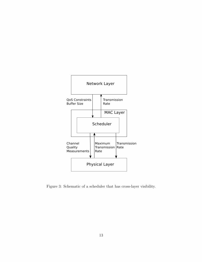
This problem is easily seen to be convex due to the joint concavity of xf(p/x) as afunction of (x, p) and also will satisfy Slater’s condition.9 Hence, it will have zeroduality gap [26, 27]. The problem (P1) can be practically motivated as follows: thephysical (PHY) layer gives the scheduler (at the MAC layer) a maximum rate that itcan serve per user based upon power and subchannel allocations, and the schedulerthen drains from the queue an amount that obeys the minimum and maximum rateconstraints (imposed by the network layer) and the maximum rate constraint fromthe PHY layer output. If the scheduler chooses not to use the complete allocationgiven by the PHY layer, then the final packet sent by the MAC layer is assumedto be constructed using an appropriate number of padded bits. However, we willnow show that at the optimal, there is no of loss optimality in assuming that thescheduler never sends less than what the PHY layer allocates, i.e., the first constraintin Problem (P1) is always made tight at an optimal solution. This point of view isexemplified in schematic shown in Figure 3.

Assume that there is an optimizer of (P1) at which for some user i, ri <∑

j xijf(pijeijxij

).

We will now construct another feasible solution that will satisfy the above relation-ship with equality. Let γ ∈ [0, 1] and set pij := γpij. Note that by convexity,both the power and subchannel constraints are satisfied for every value of γ. Now∑

j xijf(γpijeijxij

) is a non-decreasing and continuous function of γ taking values 0 at

γ = 0 and∑

j xijf(pijeijxij

) at γ = 1. Therefore, there exists a γ∗ ∈ (0, 1) such that

ri =∑

j xijf(γ∗pijeijxij

) as desired. This procedure can be followed for every user i for

whom ri <∑

j xijf(pijeijxij

), so that at the end we satisfy ri =∑

j xijf(pijeijxij

) for a

feasible (x, p). Therefore both the optimal value and an optimizer of problem (P1)

9More precisely, Slater’s condition will be satisfied provided that the minimum rate (Rmini ) are

strictly in the interior of rate-region R(e). If Rmini = 0 for all i this will trivially be true.

12

MAC Layer

Physical Layer

Scheduler

Network Layer

QoS ConstraintsBuffer Size

TransmissionRate

Channel QualityMeasurements

Maximum TransmissionRate

TransmissionRate

Figure 3: Schematic of a scheduler that has cross-layer visibility.

13

coincides with those for problem (P2). The loosest condition needed for the aboveto hold is f(·) being non-decreasing and concave with f(0) = 0. Henceforth, we willonly work with Problem (P1).

Before proceeding to solve the problem by dual methods, we first define some keynotation. For two numbers, x, y ∈ R we set x ∧ y := min(x, y), x ∨ y := max(x, y)and (x)+ = [x]+ := x ∨ 0.

3.3.1 Dual of Problem

We now proceed to derive a closed-form expression for the dual function for problem(P1). The Lagrangian obtained by relaxing the marked constraints of (P1) using thecorresponding dual variables is given by

L(r,x,p,α,µ,λ) =∑i

(wi − αi)ri +∑j

µj +M∑m=1

λmPm +∑i,j

αixijf

(pijeijxij

)−∑j

µj∑i

xij −∑m

λm∑i∈Km

∑j

pij. (12)

The corresponding dual function is then given by maximizing this Lagrangian overr,x and p. First optimizing over rate ri ∈ [Rmin

i , Rmaxi ] and noting that the La-

grangian is linear in ri we get

L(x,p,α,µ,λ) =∑i

(wi − αi)+Rmaxi −

∑i

(αi − wi)+Rmini +

∑j

µj +M∑m=1

λmPm

+∑i,j

αixijf(pijeijxij

)−∑j

µj∑i

xij −∑m

λm∑i∈Km

∑j

pij.

The optimizing r∗ is given by the following

∀i ∈ K, r∗i ∈

{Rmax

i } if αi < wi;

{Rmini } if αi > wi; and

[Rmini , Rmax

i ] if αi = wi

(13)

Note that the last term of equation (12) can be rewritten as∑m

λm∑i∈Km

∑j

pij =∑i,j

pij∑

m:i∈Km

λm =∑i,j

pijλi (14)

where λi :=∑

m:i∈Kmλm.

14

Now maximizing the Lagrangian over power p requires us to maximize

αixij

[f

(pijeijxij

)− λiαieij

pijeijxij

](15)

over pij for each i, j. From the assumptions on the function f , it is easy to check thatthe maximizing p∗ij will be of the form

p∗ijeij

xij= g

(λiαieij

)∧ sij, (16)

for some function g : R+ → [0,∞] with g(x) = 0 for x ≥ f ′(0). Specifically if df/ds

is monotonically decreasing, we may show that g(·) =(dfds

)−1(·), i.e., the inverse of

the derivative of f(·). Otherwise, since df/ds is still a non-increasing function wecan set g(x) = inf{t : df/ds(t) = x}. Using the non-increasing property of df/dswe can see that g(x) ∧ y = g

(x ∨ df

ds(y)). Note that we have assumed df/ds(0) = 1

and limt→+∞ df/ds(t) = 0 but we do not assume that lims→+∞ f(s) = +∞ (e.g., seethe self-noise example). In case f(·) is not differentiable, then we would define thefunction g(·) using the subgradients of f(·). In all cases, the key conclusion from (16)is that the optimal value of p∗ij is always a linear function of xij.

Note that when f = log(1 + 1β+1/s

), with β ≥ 0, as given by (8), then

g(x) = q((1/x− 1)+),

where

q(z) =

{z, if β = 0,(

2β+12β(β+1)

)(√1 + 4β(β+1)

(2β+1)2z − 1

), if β > 0.

Figure 4 shows p∗ij in (16) as a function of eij for the specific choice of f from (8)with three different values of β = 0, 0.01, 0.1. When β = 0, (16) becomes a “water-filling” type of solution in which p∗ij is non-decreasing in eij. For a fixed β > 0, thisis not necessarily true, i.e., due to self-noise, less power may be allocated to “better”subchannels. We also consider the case where β = 10/e to model the case whereself-noise is due to channel estimation error.

Inserting the expression for p∗ij into the Lagrangian yields

L(x,α,µ,λ) =∑i

(wi − αi)+Rmaxi −

∑i

(αi − wi)+Rmini +

∑j

µj +M∑m=1

λmPm

+∑i,j

xij

[αif

(g

(λiαieij

)∧ sij

)− λieij

(g

(λiαieij

)∧ sij

)− µj

],

(17)

15

10 12 14 16 18 20 22 24 26 28 300

0.01

0.02

0.03

0.04

0.05

0.06

0.07

Opt

imal

pow

er p

ij*

Channel condition eij (dB)

β=0

β=0.1

β=0.01

β=10/e

Figure 4: Optimal power p∗ij as a function of the channel condition eij. Here xij = 1,

αi = 1, sij = +∞, and λi = 15.

which is now a linear function of {xij}. Thus, optimizing over xij yields the dualfunction for (P1),

L(α,λ,µ) =∑i

(wi − αi)+Rmaxi −

∑i

(αi − wi)+Rmini +

∑j

µj +∑m

λmPm

+∑i,j

[αif

(g

(λiαieij

)∧ sij

)− λieij

(g

(λiαieij

)∧ sij

)− µj

]+

=∑i

((wi − αi)+R

maxi − (αi − wi)+R

mini

)+∑m

λmPm

+∑j

(∑i

[µij

(αi,

λiαieij

)− µj

]+

+ µj

), (18)

where

µij(a, b) := a

(f(g(b) ∧ sij

)− b(g(b) ∧ sij

)).

16

Note that any choice such that

x∗ij ∈

{1}, if µij

(αi,

λiαieij

)> µj,

[0, 1], if µij

(αi,

λiαieij

)= µj,

{0}, if µij

(αi,

λiαieij

)< µj

(19)

will optimize the Lagrangian in (17).

3.3.2 Optimizing the Dual Function over µ

From the duality theory of convex optimization [26,27] the optimal solution to prob-lem P1 is given by minimizing the dual function in (18) over all (α,λ,µ) ≥ 0. We dothis coordinate-wise starting with the µ variables. The following lemma characterizesthis optimization.

Lemma 1 For all α,λ ≥ 0,

L(α,λ) := minµ≥0

L(α,λ,µ)

=∑i

((wi − αi)+R

maxi − (αi − wi)+R

mini

)+∑m

λmPm +∑j

µ∗j(α,λ),

(20)

where for every tone j, the minimizing value of µ∗j is achieved by

µ∗j(α,λ) := maxiµij

(αi,

λiαieij

). (21)

The proof of Lemma 1 follows from a similar argument as in [9]. Note that (21)requires searching for the maximum value of the metrics µij across all users for eachtone j. Since L(α,λ) is the minimum of a convex function over a convex set, it is aconvex function of (α,λ).

3.3.3 Optimizing the Dual Function over (α,λ)

Now we are ready to optimize the remaining variables in the dual functions, namely,(α,λ). In the single cell downlink case with no rate constraints (and thus no α vari-ables), this reduces to a one dimensional problem in λ and hence, it can be minimizedusing an iterated one dimensional search (e.g., the Golden Section method [26]). Sincethere is no duality gap, at λ∗ = arg minλ≥0 L(λ), L(λ∗) gives the optimal objective

17

value of problem (P1). Similarly, in the absence of rate constraints, the multiplesites/sectors problem with a partition of the users {Km}Mm=1 also leads to a one di-mensional problem within each partition.

In general, however, one would need to use subgradient methods [26, 27] to nu-merically solve for the optimal (α,λ). The following lemma characterizes the set ofsubgradients of L(α,λ) with respect to (α,λ).

Lemma 2 About any (α0,λ0) ≥ 0,

L(α,λ) ≥∑i

d(α0i )(αi − α0

i ) +∑m

d(λ0m)(λm − λ0

m), (22)

with

d(λm) = Pm −∑i∈Km

p∗ij = Pm −∑i∈Km

x∗ijeijg

(λiαieij

)∧ sij (23)

d(αm) =∑j

x∗ijf

(g( λiαieij

)∧ sij

)− r∗i (24)

where x∗ijs satisfy∑i

x∗ij ≤ 1 and µj(α,λ)

(1−

∑i

x∗ij

)= 0; ∀j,

and satisfy the equation (19) with µj = µ∗j(α,λ) as given in equation (21), and r∗isatisfy equation (13). Thus the subgradients d(λm) and d(αi) are parameterized by(r∗,x∗) and are linear in these variables. Moreover, the permissible values of r∗ liein a hypercube and those of x∗ in a simplex.

Observe that the dual function at any point (α,λ) is obtained by taking themaximum of the Lagrangian over (r∗,p∗,x∗) satisfying

∑i xij ≤ 1,∀j ∈ N , (x,p) ∈

X . In case (r∗,p∗,x∗) is unique, then the resulting Lagrangian is a gradient tothe dual function at (α,λ). In case there are multiple optimizers, the resultingLagrangians are each a subgradient, and every subgradient can be obtained by aconvex combination of these subgradients so that the set of subgradients is convex.The lemma follows easily by substituting for the optimal (r∗,p∗,x∗).

Having characterized the set of subgradients, a method similar to that used in [25]for the single cell uplink problem can be used to solve for the optimal dual variables(α∗,λ∗) numerically. In each step of this method we change the dual variables alongthe direction given by a subgradient subject to non-negativity of the dual variables.The convergence of this procedure (for a proper step-size choice) is once again guar-anteed by the convexity of L(α,λ) (see [26, Exer. 6.3.2], [25]).

18

3.3.4 Optimizing the dual function over α

Since the dimension of α equals the number of users and the dimension of µ equalsthe number of tones, it may be computationally better to optimize over α insteadof µ if the number of users is greater, and then use numerical methods to solve theproblem. Next we detail the means to optimize over α before µ. The dual functioncontains many terms that have definitions with (·)+, and therefore we would need toidentify exactly when these terms are non-zero. For this we need to solve a non-linearequation which is guaranteed to have a unique solution. We first discuss this andthen apply it to optimizing the dual function over α.

Given y, z ≥ 0, define by v(y, z) the unique solution with 1 ≤ x < +∞ to

xf

(g(1

x∨ dfds

(z)))− g(1

x∨ dfds

(z))

= y,

where it is easy to show that xf

(g(

1x∨ df

ds(z)))− g(

1x∨ df

ds(z))

is a monotonically

increasing function taking value 0 at x = 1 and increasing without bound as x→ +∞.

If y ≥ f(z)/(df/ds(z))−z(≥0)

, then v(y, z) = (y+z)/f(z) where it is easy to verify

that v(y, z) ≥ z/f(z) ≥ 1/(df/ds(z)) ≥ 1/(df/ds(0)) = 1 from the concavity of f(·)and from f(0) = 0. Otherwise we need to solve for the unique 1 ≤ x ≤ 1/(df/ds(z))such that

xf

(g(1

x

))− g(1

x

)= y.

For our results we will be interested in v(µjeij

λi, sij

), using which we also define

νij :=λiv(µjeij

λi, sij

)eij

and ζij :=µj +

sij λieij

f(sij),

where νij = ζij ifµjeij

λi≥ f(sij)

df(sij)

ds

− sij.

First note that we can rewrite the function in (18) as follows

L(α,µ,λ) =∑j

µj +∑m

λmPm +∑i

Li,

where Li = (wi − αi)+Rmaxi − (αi − wi)+R

mini

+∑j

λieij

[αieij

λif

(g( λiαieij

)∧ sij

)−(g( λiαieij

)∧ sij

)− µjeij

λi

]+

.

19

Now using the quantities defined earlier in this section, one can write Li as follows

Li =∑j

λieij

[1{0≤αi≤ζij}

(αieijλi

f(sij)− sij −µjeij

λi

)+

1{ζij<αi≤νij}

(αieij

λif

(g( λiαieij

))− g( λiαieij

)− µjeij

λi

)]+ (wi − αi)+R

maxi − (αi − wi)+R

mini .

Minimizing Li over αi ≥ 0 can now be accomplished by a simple one dimensionalsearch; we define the optimal vector of αis to be α∗(λ,µ). Thereafter one wouldneed to use a subgradient method [25, 26] to numerically minimize over (µ,λ). Asubgradient of L with respect to λm is given by Pm −

∑i∈Km

p∗ij where p∗ij is taken

from (16) where one substitutes x∗ij from (19). A subgradient of L with respect to µjis given by 1 −

∑i x∗ij where we substitute for x∗ij from (19). Note, however, that it

is important that we also meet the following constraints for all i, namely,

Rmini ≤

∑i

x∗ijf

(p∗ijx∗ij

)≤ Rmax

i ;

if α∗i < wi, then∑j

x∗ijf

(p∗ijx∗ij

)= Rmax

i ; and

if α∗i > wi, then∑j

x∗ijf

(p∗ijx∗ij

)= Rmin

i .

The proof of this follows by retracing the steps of the proof of Lemma 2 with theroles of α and µ being switched.

3.4 Primal optimal solution

For the general OFDMA problem we presented two methods to solve for V ∗: in thefirst method we showed how to characterize the dual variables µ(α,λ) and then weproposed numerically solving for the optimal (α∗,λ∗) using subgradient methods,while in the second method followed the same strategy after switching the roles of µand α. However, we still need to solve for the values of the corresponding optimalprimal variables. Concentrating on the first method, we know by duality theory [26]that given (α∗,λ∗) we need to find one vector from the set of (r∗,x∗,p∗) that alsosatisfies primal feasibility and complementary slackness. These constraints can easilybe seen to translate to the following:

d(λ∗m) ≥ 0, d(λ∗m)λ∗m = 0, ∀m; (25)

d(α∗i ) ≥ 0, d(α∗i )α∗i = 0, ∀i. (26)

20

From the linearity of d(λ∗m), d(α∗i ) in (r∗,x∗) it follows that the primal optimal(r,x,p) are the solution of a linear program in (r∗,x∗).

For the single cell downlink case with no rate constraints, as we have previouslynoted searching for the dual optimal is a one dimensional numerical search in λ. Inthat case, the search for primal optimal solution turns out to have additional structureas shown in [28].

3.5 OFDMA Feasibility

Next we turn to the corresponding feasibility problem, which can be stated as:

V ∗ = minσ (27)

subject to: Ri ≤∑j

xijf(pijeijxij

), ∀ i (αi)∑i

xij ≤ 1 ∀ j (µj)∑i∈Km

∑j

pijPm≤ σ ∀ m (λm)

(x,p) ∈ X .

The vector of rates (Ri) is feasible if V ∗ ≤ 1, i.e., all the power constraints willalso be satisfied by a vector (x∗,p∗). As mentioned earlier, we need to check that(Ri) = (Rmin

i ) is indeed feasible; otherwise problems (P1) and (P2) are both infeasibleas well. Moreover, if (Ri) = (Rmax

i ) is also feasible, then r = (Rmaxi ) is the optimizer

for problems (P1) and (P2). In which case, the optimal solution to the problem abovewith (Ri) = (Rmax

i ) will also yield an optimal solution to the scheduling problem.Observe that problem (27) is convex and satisfies Slater’s conditions. Finally, we alsonote that other alternate formulations of the feasibility problem are possible whereone could either apply the σ constraint also on the subchannel utilization or switch theroles of subchannel and power utilization. All of these will yield the same conclusionabout feasibility although the actual solutions, in terms of (x∗,p∗), would possiblybe different.

The Lagrangian considering the marked constraints is

L(σ,x,p,α,µ,λ) = σ

(1−

∑m

λm

)−∑j

µj +∑i

αiRi

+∑ij

µjxij −∑ij

(αixijf

(pijeijxij

)+ pijλi

)

21

where λi :=∑

m:i∈Km

λmPm

. As before, minimizing over pij yieldsp∗ijeij

xij= g

(λiαieij

)∧ sij.

Substituting this in the Lagrangian, we get

L(σ,x,α,µ,λ) =∑i

αiRi −∑j

µj + σ

(1−

∑m

λm

)

−∑i,j

xij

[αif(g(

λiαieij

) ∧ sij)−λieij

(g(λiαieij

) ∧ sij)− µj

].

Minimizing over 0 ≤ xij ≤ 1 yields

L(σ,α,µ,λ) =∑i

Li −∑j

µj + σ

(1−

∑m

λm

)

where

Li = αiRi −∑j

[αif(g(

λiαieij

) ∧ sij)−λieij

(g(λiαieij

) ∧ sij)− µj

]+

.

Next we minimize L over all values of σ. Since there are no constraints on σ, itfollows that the resulting L is finite only when

∑m λm = 1; for all other values we

would get L = −∞. Hereafter we will assume that∑

m λm = 1. Thus

L(σ,x,α,µ,λ) =∑i

Li −∑j

µj.

Note that as before, as a function of αi the problem is now separable. Therefore weonly need to maximize Li over αi ≥ 0.

Similarly we can write L as

L(σ,x,α,µ,λ) =∑j

Lj +∑i

αiRi,

where we have

Lj = −

(µj +

∑i

[αif(g(

λiαieij

) ∧ sij)−λieij

(g(λiαieij

) ∧ sij)− µj

]+

)

As a function of µj the problem is now separable, and we only need to maximize Ljover µi ≥ 0.

22

Thus, we could optimize first over either µ or α, once again based upon whetherthe number of users or subchannels is smaller. In either case, the methodology and thefunctions that appear are very similar to the corresponding problem in the schedulingproblem (P1), and due to space constraints we do not elaborate on this. Care mustbe take, however, while evaluating subgradients with respect to λ. Here we proposeusing a projected gradient method [26, 27] based upon the constraint

∑m λm = 1 to

numerically solve for the optimal λ.

3.6 Power allocation given subchannel allocation

In many of the suboptimal scheduling algorithms that we will discuss, a central featurewill be a computationally simpler (but still close to optimal) method to provide asubchannel allocation. Once the subchannel allocation has been made, all that willremain is the power allocation problem, subject to the various constraints that wediscussed earlier. Here we discuss how this can be solved in an optimal manner. Asimilar question can also be asked about the feasibility problem, hence we also discussthis here. In all cases, we assume that we are given a feasible subchannel allocation.

Since we are given a feasible subchannel allocation x, the Lagrangian of the newscheduling problem (power allocation only) can be easily derived by setting µ = 0.For this we once again use the formulation based upon Problem (P1). The optimal

power allocation is then given by p∗ij =xijeij

(g(

λiαieij

)∧ sij

). The Lagrangian that

results from substituting this formula is

L(x,α,λ) =∑m

λmPm +∑i

(wi − αi)+Rmaxi −

∑i

(αi − wi)+Rmini

+∑i

∑j

αixijf

(g( λieijαi

)∧ sij

)− λixij

eij

(g( λieijαi

)∧ sij

).

Now it is easy to argue that if Rmini = 0 and Rmax

i = +∞ and if the Kms form apartition, then within each partition the λms can be solved for as in Section 3.3. Inany case, in this setting solving for the optimal αi ≥ 0 is easier, but uses some ofthe functions described at the end of Section 3.3. However, after this step we wouldstill need to solve for λ numerically; if the partitions assumption holds, then it wouldonly need a single dimensional search within each partition. A finite-time algorithmfor achieving the optimal λ has been given in [25,28] under the assumption that f(·)represents the Shannon capacity as in (8) with β = 0.

23

3.6.1 Feasibility check

Under the assumption that a feasible subchannel allocation has already been provided,even the feasibility check problem becomes a lot easier. As before we can assume∑

m λm = 1, and that the optimal power allocation is given by p∗ij =xijeij

(g(

λieijαi

)∧sij

),

and substituting this we get

L(x,α,λ) =∑i

αiRi −∑j

xij

[αif

(g( λieijαi

)∧ sij

)− λieij

(g( λieijαi

)∧ sij

)].

Again solving for the optimal αi is simpler. Once again the λ vector would need tobe computed numerically, subject to it being a probability vector, i.e.,

∑m λm = 1

and λm ≥ 0 for each m.

4 Low Complexity Suboptimal Algorithms with

Integer Channel Allocation

There are two shortcomings with using the optimal algorithm outlined in the previ-ous section for scheduling and resource allocation: (i) the complexity of the algorithmin general is not computationally feasible for even moderate sized systems; (ii) thesolution found may require a time-sharing channel allocation, while practical imple-mentations typically require a single user per sub-channel. One way to address thesecond point is to first find the optimal primal solution as in the previous section andthen project this onto a “nearby” integer solution. Such an approach is presentedin [28] for the case of a single cell downlink system (M = 1) without any rate con-straints. In that setting, after minimizing the dual function over µ, one optimizesthe function L(λ), which only depends on a single variable. This function will havescalar subgradients which can then be used to develop rules for implementing suchan integer projection. Moreover, in this case since L(λ) is a one-dimensional functionthe search for the optimal dual values is greatly simplified. However, in the generalsetting, this type of approach does not appear to be promising.10

In this section we discuss a family of sub-optimal algorithms (SOA’s) for thegeneral setting that try to reduce the complexity of the optimal algorithm, while sac-rificing little in performance. These algorithms seek to exploit the problem structurerevealed by the optimal algorithm. Furthermore, all of these sub-optimal algorithmsenforce an integer tone allocation during each scheduling interval. In the followingwe consider the general model from Section 3.1 with the restriction that {Km} forms

10See [25] for a more detailed discussion of this in the context of the uplink scenario.

24

a partition of the user groups (i.e. each user is in only one of these sets) and thatRmini = 0 for all i. In a typical setting both of these assumptions will be true.

In the optimal algorithm, given the optimal λ and α, the optimal tone alloca-tion up to any ties is determined by sorting the users on each tone according to the

metric µij(αi,λiαieij

) (cf. (19)). Given an optimal tone allocation, the optimal power

allocation is given by (16). In each SOA, we use the same two phases with somemodifications to reduce the complexity of computing (λ, α) and the optimal tone al-location. Specifically, we begin with a subChannel Allocation (CA) phase in which weassign each tone to at most one user. We consider two different SOAs that implementthe CA phase differently. In SOA1, instead of using the metric given by the optimalλ and α, we consider metrics based on a constant power allocation over all tonesassigned to a partition. In SOA2, we find the tone allocation, once again througha dual based approach, but here we first determine the number of tones assigned toeach user and then match specific tones and users. In all cases we assign the tones todistinct partitions which will, in turn, yield an interference-free operation. After thetone allocation is done in both SOAs, we execute the Power Allocation (PA) phasein which each user’s power is allocated across the assigned tones using the optimalpower allocation in (16).

4.1 CA in SOA1: Progressive Subchannel Allocation Basedon Metric Sorting

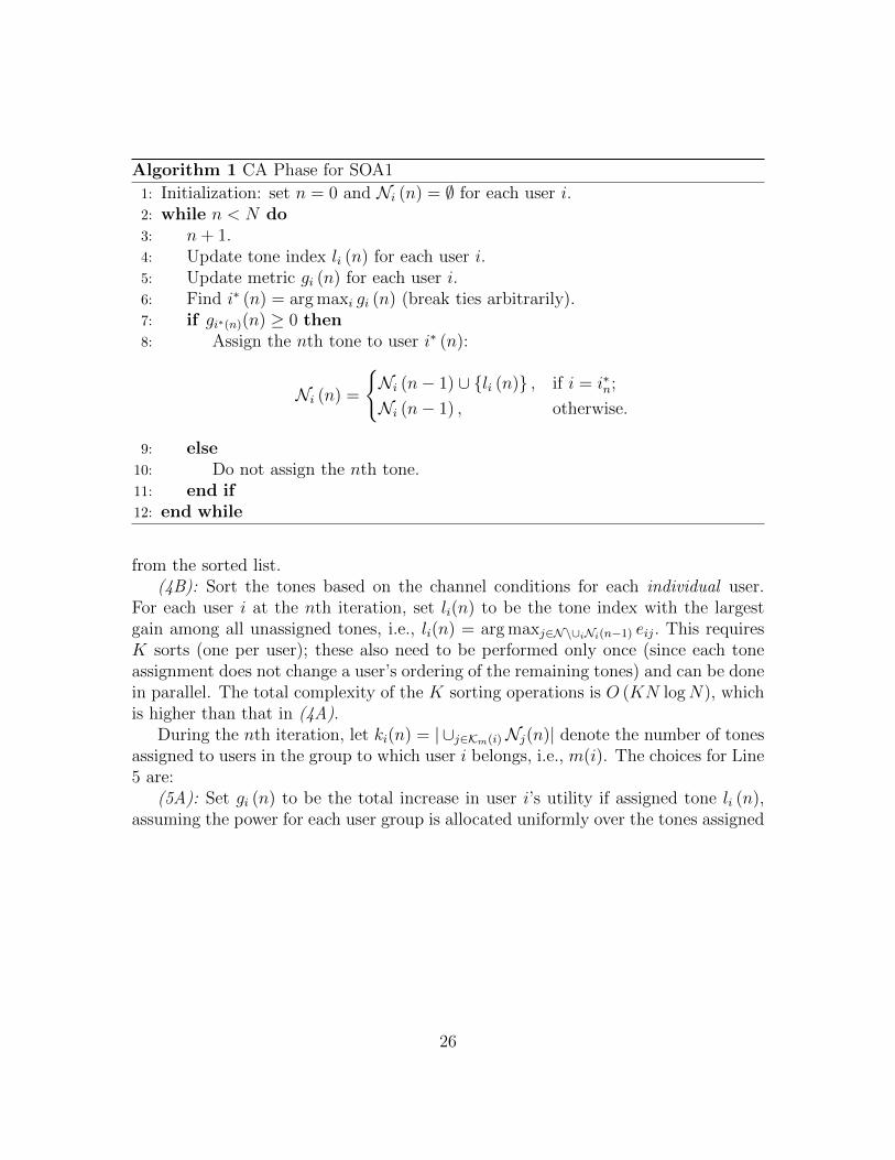
In this family of SOAs, tones are assigned sequentially in one pass based on a peruser metric for each tone, i.e., we iterate N times, where each iteration correspondsto the assignment of one tone. Let Ni(n) denote the set of tones assigned to user iafter the nth iteration. Let gi(n) denote user i’s metric during the nth iteration andlet li(n) be the tone index that user i would like to be assigned if he/she is assignedthe nth tone. The resulting CA algorithm is given in Algorithm 1. Note that all theuser metrics are updated after each tone is assigned.

We consider several variations of Algorithm 1 which correspond to different choicesfor steps 4 and 5. The choices for step 4 are:

(4A): Sort the tones based on the best channel condition among all users. Thisinvolves two steps. First, for each tone j, find the best channel condition amongall users and denote it by µj := maxi eij. Second, find a tone permutation {αj}j∈Nsuch that µα1 ≥ µα2 ≥ · · · ≥ µαN

, and set li (n) = αn for each user i at the nthiteration. Each max operation has complexity of O(K), and the sorting operationhas a complexity of O(N log(N)). The total complexity is O (NK +N logN). Wenote that this is a one-time “pre-processing” that needs to done before the CA phasestarts. During the tone allocation iterations, the users just choose the tone index

25

Algorithm 1 CA Phase for SOA1

1: Initialization: set n = 0 and Ni (n) = ∅ for each user i.2: while n < N do3: n+ 1.4: Update tone index li (n) for each user i.5: Update metric gi (n) for each user i.6: Find i∗ (n) = arg maxi gi (n) (break ties arbitrarily).7: if gi∗(n)(n) ≥ 0 then8: Assign the nth tone to user i∗ (n):

Ni (n) =

{Ni (n− 1) ∪ {li (n)} , if i = i∗n;

Ni (n− 1) , otherwise.

9: else10: Do not assign the nth tone.11: end if12: end while

from the sorted list.(4B): Sort the tones based on the channel conditions for each individual user.

For each user i at the nth iteration, set li(n) to be the tone index with the largestgain among all unassigned tones, i.e., li(n) = arg maxj∈N\∪iNi(n−1) eij. This requiresK sorts (one per user); these also need to be performed only once (since each toneassignment does not change a user’s ordering of the remaining tones) and can be donein parallel. The total complexity of the K sorting operations is O (KN logN), whichis higher than that in (4A).

During the nth iteration, let ki(n) = | ∪j∈Km(i)Nj(n)| denote the number of tonesassigned to users in the group to which user i belongs, i.e., m(i). The choices for Line5 are:

(5A): Set gi (n) to be the total increase in user i’s utility if assigned tone li (n),assuming the power for each user group is allocated uniformly over the tones assigned

26

to that group, i.e.,

gi(n) =

wi

[(∑j∈Ni(n−1)∪{li(n)} f

(Pieij

ki(n−1)+1∧ sij

))∧Rmax

i

−

(∑j∈Ni(n−1) f

(Pieij

ki(n−1)∧ sij

))∧Rmax

i

] ,if ki(n− 1) > 0;

wi

[(∑j∈Ni(n−1)∪{li(n)} f

(Pieij

ki(n−1)+1∧ sij

))∧Rmax

i

],otherwise.

(28)

(5B): Set gi (n) to be user i’s gain from only tone li (n), again assuming constantpower allocation within each group, i.e.

gi (n) = wi

[f

(Piei,li(n)

ki(n− 1) + 1∧ sij

)∧Rmax

i

].

Compared with (5A), this metric is simpler to calculate but ignores the change inuser i’s utility due to the decrease in power allocated to any tones in Ni(n − 1). Italso does not accurately enforce the maximum rate constraint, since it only considersone tone at a time.

The complexity of either of these choices over N iterations is O(NK), and sothe total complexity for the CA phase is O (NK +N logN) (if (4A) is chosen) orO (KN logN) (if (4B) is chosen). Algorithms similar to SOA1 with (4B) and (5B)have been proposed in the literature for both the single cell downlink setting [12]11 andthe uplink [36] without rate or SNR constraints. In the single cell downlink case, thealgorithm in [12] is shown via numerical examples to have near optimal performance.In the uplink case, this also performs reasonably well in simulations [36], but [25]shows that better performance can be obtained using (4B) and (5A) instead.

4.2 CA in SOA2: tone Number Assignment & tone UserMatching

SOA2 implements the CA phase through two steps: tone number assignment (CNA)and tone user matching (CUM). The algorithm is summarized in Algorithm 2.

11The main difference with the algorithm in [12] is that after each iteration n, it then checks tosee if

∑i wiri is increasing and if not it stops at iteration n − 1. Such a step can be added to

Algorithm 1; however, unless the system is lightly loaded it is unlikely to have a large impact on theperformance.

27

Algorithm 2 CA Phase of SOA2

1: subChannel Number Assignment (CNA) step: determine the number of tones niallocated to each user i such that

∑i∈K ni ≤ N .

2: subChannel User Matching (CUM) step: determine the tone assignment xij ∈{0, 1} for all users i and tones j, such that

∑j∈N xij = ni.

4.2.1 subChannel Number Assignment (CNA)

In the CNA step, we determine the number of tones ni assigned to each user i ∈ K.The assignment is calculated based on the approximation that each user sees a flatwide-band fading tone. Notice that here we do not specify which tone is allocatedto which user; such a mapping will be determined in the CUM step. The CNAstep is further divided into two stages: a basic assignment stage and an assignmentimprovement stage.

Stage 1, Basic Assignment : Here, the assignment is based on the normalized SNRaveraged over all tones. Specifically, we model each user i as having a normalizedSNR ei = 1

N

∑j∈N eij, and then determine a tone number assignment ni for all i by

solving:

max{ni≥0,i∈K}

∑i∈K

winif

(Pm(i)ei∑j∈Km(i)

nj∧ si

)subject to:

∑i∈K

ni ≤ N

nif

(Pm(i)ei∑j∈Km(i)

nj∧ si

)≤ Rmax

i .

(SOA2-CNA)

Here, we are again assuming that power is allocated uniformly over all the channelsassigned to a given user group.

Unfortunately, in general the objective in Problem SOA2-CNA is not concave.However, in the special case of the uplink (Km(i) = {i}) it will be.12 In the caseof the single cell downlink, if nf(a/n) is increasing for all a > 0 (as in our generalformulation), then the problem can be re-formulated to have a concave objectiveby noting that in this case it must be that

∑i∈K ni = N at any optimal solution.

Additionally, due to the maximum rate constraint, the constraint set may not beconvex; this can be accommodated by considering a higher dimensional problem asin Section 3.3.

12Some care is required at the point where the SNR constraint becomes active as the objective isnot differentiable there; nevertheless, by evaluating left and right derivatives the concavity can beshown.

28

Next, we focus on solving Problem SOA2-CNA in the uplink setting withoutmaximum rate constraints. In this case, the problem will have a unique and possiblynon-integer solution, which we can again use a dual relaxation to find. Consider theLagrangian

L(n, λ) :=∑i∈K

winif

(Pieini∧ si

)− λ

(∑i∈K

ni −N

).

Optimizing L(n, λ) over n ≥ 0 for a given λ is equivalent to solving the following Ksubproblems,

n∗i (λ) = arg maxni≥0

winif

(Pieini∧ si

)− λni,∀i. (29)

Problem (29) can be solved by a simple line search over the range of (0, N ]. Substi-tuting the corresponding results into the Lagrangian yields

L(λ) :=∑i∈K

win∗i (λ) f

(Piein∗i (λ)

∧ si)− λ

(∑i∈K

n∗i (λ)−N

),

which is a convex function of λ [26]. The optimal value

λ∗ = arg minλ≥0

L(λ) (30)

can be found by a line section search over: [0,maxiwif( PieiN/K

)]13. For a given search

precision, the maximum number of iterations needed to solve either (29) or (30) isfixed.14. Hence, the worst case complexity of the solving each subproblem is inde-pendent of K or N . Since there are K subproblems in (29), it follows that thecomplexity of the basic assignment step is O(K). If the resultant channel alloca-tions contain non-integer values, we will approximate with an integer solution thatsatisfies

∑i∈K ni = N .15 Since each user is allocated only a subset of the tones, the

normalized SNR ei = 1N

∑j∈N eij is typically a pessimistic estimate of the averaged

13The upperbound of the search interval can be obtained by examining the first order optimalitycondition of (29).

14For example, if we use bi-section search to solve (29) and stop when the relative error of thesolution is less than N/210, then we only need a maximum of ten search iterations.

15One possible integer approximation is the following. Assume n∗i is the unique optimal so-lution of Problem SOA2-CNA. First, sort users in the descending order of the mantissa ofn∗i , fr (n∗i ) = n∗i − bn∗i c. That is, find a user permutation subset {αk, 1 ≤ k ≤ N} such thatfr(n∗α1

)≥ fr

(n∗α2

)≥ · · · ≥ fr

(n∗αM

). Second, for each user i, let n∗i = bn∗i c. Third, calcu-

late the number of unallocated tones, NA = N −∑i n∗i . Finally, adjust users with large mantissas

such that all the tones are allocated, i.e., n∗αi= n∗αi

+ 1 for all 1 ≤ i ≤ NA. The resulting {n∗i }i∈Kgive the integer approximation.

29

tone conditions over the allocated subset. This motivates us to consider the followingassignment improvement stage of CNA.

Stage 2, Assignment Improvement : Here, assignment is performed by means ofiterative calculations using the normalized SNR averaged over the best tone subset.Specifically, we iteratively solve the following variation of Problem SOA2-CNA (statedhere for the uplink without maximum rate constraints):

maxn(t)≥0

∑i∈K

wini(t)f

(Piei (t)

ni(t)∧ si

)subject to:

∑i∈K

ni (t) ≤ N

nif

(Pm(i)ei (t)∑j∈Km(i)

nj∧ si

)≤ Rmax

i ,

(SOA2-CNA-t)

for t = 1, 2, .... During the t-th iteration, ei (t) is a refined estimate of the normalizedSNR based on the best bni (t− 1)c (or dni (t− 1)e) tones of user i; additionally,ni(0) := N for all i. The iteration stops when the tone allocation converges or themaximum number of iterations allowed is reached. An integer approximation will beperformed if needed.

The complete algorithm for the CNA phase of SOA2 is given in Algorithm 3.In order to perform the assignment improvement, we need to perform K sortingoperations, with a total complexity O(KN log(N)). Note that this only needs tobe done once. Step 4 of each iteration has complexity of O(K) due to solving Ksubproblems for a fixed dual variable. The maximum number of iterations is fixedand thus is independent of N or K. The integer approximation stage requires asorting with the complexity of O(K log(K)). So the total complexity for the CNAphase of SOA2 is O(KN log(N) +K log(K)).

Algorithm 3 CNA Phase of SOA2

1: Initialization: integer MaxIte> 0, t = 0, ni(0) = N and ni(1) = N/2 for eachuser i.

2: while (ni (t+ 1) 6= ni (t) for some i) & (t <MaxIte) do3: t = t+ 1.4: For each user i, ei (t) = average gain of user i’s best ni (t− 1) tones.5: Solve Problem (SOA2-CNA-t) to determine the optimal ni (t) for each user i.6: end while7: let n∗i = ni(t) for each user i.

30

4.2.2 subChannel User Matching (CUM) Step

After the CNA step, we know how many tones are to be allocated to each user.However, we still need to determine which specific tones are assigned to which user.This is accomplished in the CUM step by finding a tone assignment that maximizesthe weighted-sum rate assuming each user employs a flat power allocation, i.e. wesolve the problem:

maxxij∈{0,1}

∑i∈K

∑j∈N

xijwif

(Pieijn∗i∧ si

)subject to:

∑j∈N

xij = n∗i ,∀i ∈ K,∑i∈K

xij = 1,∀j ∈ N ,

(SOA2-CUM)

where n∗ = (n∗i , i ∈ K) is the integer tone allocation obtained in the CNA step. Sincewe solved Problem (SOA2-CNA-t) using the average of the best n∗, then concavity off(·) ensures that any feasible tone allocation for Problem (SOA2-CUM) will satisfythe maximum rate constraint.

Problem SOA2-CUM is an integer Assignment Problem whose optimal solutioncan be found by using the Hungarian Algorithm [30].16 To use the Hungarian algo-rithm here, we need to perform “virtual user splitting” as explained next. For user i,

let rij = wif(Pieijn∗i∧ sij

), and let

ri = [ri1, ri2, · · · , riN ]

be user i’s achievable rates over all possible tones. We can then form a K × N

matrix R =[rT1 , r

T2 , · · · , rTM

]T. Next, we split each user i into n∗i virtual users by

adding n∗i − 1 copies of the row vector ri to the matrix R. This expands R into aN × N square matrix. Solving Problem SOA2-CUM is then equivalent to finding apermutation matrix C∗ = [cij]N×N such that

C∗ = arg minC∈C−C ·R := arg min

C∈C−

N∑i=1

N∑j=1

cijrij. (31)

Here C is the set of permutation matrices, i.e., for any C ∈ C, we have cij ∈ {0, 1},∑i cij = 1 and

∑j cij = 1 for all i and j. This problem can be solved by the standard

16A similar idea has been used to solve various single cell downlink OFDMA resource allocationproblems (e.g., [18]) as well as to find user coalitions for Nash Bargaining in an uplink OFDMAsystem in [32].

31

Hungarian algorithm which has a computational complexity of O (N3), where N is thetotal number of tones. The detailed algorithm can be found in [30]. After obtainingC∗, we can calculate the corresponding tone allocation x∗. For example, if c∗kj = 1and virtual user k corresponds to the actual user i, then we know x∗ij = 1, i.e., tonej is allocated only to user i.

4.3 Power Allocation (PA) phase

We can follow the tone allocation (CA) phase in either SOA1 and SOA2 with a powerallocation phase in which power is optimally allocated among the tones assigned tothe users in each partition.17 After this optimization it is possible that some toneis allocated zero power due to its poor tone gain. Alternatively, one can simply usea uniform power allocation as was assumed in the CA phase. For certain single celldownlink scenarios, such a uniform allocation has been shown to be nearly optimalin [12,28].

Since the tone allocation is given, optimizing the power allocation for each groupis equivalent to the problem considered in Section 3.6 and can be addressed in a sim-ilar way, i.e. by considering the dual formulation and numerically searching for theoptimal dual variables. We note that in the uplink scenario without any maximumrate constraint, we need to solve one such problem for each user and for each prob-lem only a single dual variable needs to be introduced (corresponding to the user’spower constraint). Hence, the optimal dual value can be found through a simple linesearch, with a constant worst-case complexity given a fixed search precision as in ourdiscussion of (29).

4.4 Complexity and performance of Suboptimal Algorithmsfor the Uplink Scenario

In this section we discuss the complexity and performance of the suboptimal algo-rithms in an uplink scenario without any maximum rate constraints 18. The worstcase computational complexities of the variations of SOA1 and SOA2 for this settingare summarized in Table 1.

Next we briefly discuss the performance of this algorithms with a realistic OFDMAsimulator assuming parameters and assumptions commonly found in the IEEE 802.16standards [10]. These results are for a single cell with 40 users. All users are infinitelyback-logged and assigned a throughput-based utility as in (3) with parameter ci = 1

17In this section, we again consider the case where {Km} forms a partition of the users and allowfor maximum rate constraints.

18It can be argued that this will also be the worst-case setting for the general problem assumingpartitions and no rate constraints.

32

Table 1: Worst Case Computational Complexity of Suboptimal Algorithms

Suboptimal Algorithm Worst Case Complexity

4A & 5A O (NK +N logN)subChannel Allocation (CA) 4A & 5B O (NK +N logN)

4B & 5A O (KN logN)SOA1 4B & 5B O (KN logN)

Power Allocation (PA) O (KN)Total (CA + PA) O (KN logN)

subChannel Allocation (CA) CNA O (KN logN +K logK)CUM O (N3)

SOA2 Power Allocation (PA) O (KN)Total (CA+PA) O (N3 +KN logN +K logK)

and α = 0.5. Each user i has a total transmission power constraint Pi = 2W. Wecalculate the achievable rate of user i on tone j as

rij = Bxij log

(1 +

pijeijxij

),

where B is the tone bandwidth and eij is generated according to a product of a fixedlocation-based term and a frequency-selective fast fading term. A detailed descriptionof the simulation set-up can be found in [25] with further results. Scheduling decisionsare made every 20 OFDM symbols, which corresponds to one fading block.

Table 2 shows simulation results for the following four algorithms:

1. Integer-Dual: integer tone allocation (with tie breaking) based on optimal dual-based algorithm and optimal power control. To reduce computational complex-ity in the case of too many ties, we randomly inspect up to 128 ways of breakingthe ties with an integer allocation and select the allocation among these withthe largest weighted sum rate (before reallocating the power).

2. SOA1: tone allocation as in Section 4.1 and power control as in Section 4.3.There are four versions of SOA1, depending on how steps 4 and 5 in Algorithm1 are implemented; we present results for each.

3. SOA2: tone allocation as in Section 4.2 (with up to 10 iterations) and powercontrol as in Section 4.3.

33

Table 2: Example Uplink resource allocation performance

Algorithms Utility Log U Rate Scheduled Users

Integer-Dual 53922 514.0 21.56 37.54A & 5A 52494 510.7 22.86 34.6

SOA 1 4A & 5B 51697 509.2 20.22 28.14B & 5A 54165 513.3 22.25 35.04B & 5B 53156 511.4 21.43 28.6

SOA 2 54316 513.6 22.33 35.1Base Line 21406 -1960.5 16.13 2.66

4. Base-line: each tone j is allocated to the user i with the highest eij, withoutconsidering the weights wi’s and the power constraints. Each user’s power isthen allocated as in Section 4.3.

In this table it can be seen that SOA1 (with 4B & 5A) and SOA2 achieve thebest performance in terms of total utility. Their performance is even better than theInteger-Dual approach, which was obtained based on the optimal value of the relaxedproblem. This is likely because only 128 ways to break ties are considered whichis typically not sufficient. Since the Integer-Dual algorithm achieves an optimalityratio of 0.9412, this suggests that SOA1 and SOA2 achieve very close to optimalperformance as well. The base-line algorithm always has poor performance.

Here, and in other uplink simulation reported in [25], all of the SOAs have goodperformance with SOA1 (with 4B & 5A) and SOA2 consistently achieving the bestperformance in terms of total utility. From Table 1, we note that these have slightlyhigher complexity than some of the other SOAs. Hence if lower complexity is desired,this can be provided with only a slight loss in performance. We also note that ineach case the SOAs and the integer-dual algorithm schedule a large number of userson average in each time-slot. A potential cost from this is that it may increase theneeded signaling overhead. One way to reduce this cost is to add a penalty term toour objective which increases with the number of users scheduled.

5 Conclusions and Open Problems

In this chapter, we have considered a general model of gradient-based scheduling andresource allocation for OFDMA systems. This model includes single cell downlink,uplink, and multi-cell downlink with frequency sharing, and incorporates various

34

practical constraints such as per carrier SNR constraints, self-noise due to imper-fect channel estimates or phase noise, and minimum and maximum per user rateconstraints. Essentially the problem can be reduced to solving a weighted rate maxi-mization problem in each time-slot. We address this problem with a Lagrangian dualrelaxation method. By exploiting the structure of the OFDMA rate region, we canexpress the dual function in terms of a small subset of dual variables. The optimalvalues of these variables can be found through standard numerical search methods.An interesting observation is that recovering the optimal primal solutions given opti-mal dual variables is rather straightforward in most cases, since the optimal channelallocations often turn out to be integer “automatically”. In the case when this isnot true, we need to calculate the channel allocation by either allowing time-sharingor picking a good integer solution, and optimize the power allocation accordingly.Based on the intuition derived from the optimal algorithms, we demonstrate that itis possible to design a class of heuristic algorithms that are low in complexity butperform very well in simulation studies.

All algorithms presented in this chapter are centralized. This is not an issue for thesingle cell downlink case or even for a multi-sectored site, where the resource allocationdecisions are made by the base station. In the uplink and multi-cell downlink cases,however, a distributed algorithm is more desirable since the decisions are made bythe multiple network entities (either multiple mobile users or multiple base stations).Some preliminary results towards a fully distributed algorithm have been reportedin [40,41] and more work is needed along this line. Another open issue regarding themulti-cell downlink case is to consider models which allow dynamic frequency re-use.A challenge in such settings is that the resulting optimization problem may not longerbe convex even when the integer constraints are relaxed.

The algorithms presented here require assume that the scheduler has accuratechannel quality information (though some inaccuracy may be accounted for via theself-noise terms). In OFDMA systems with many users and tones, the resultingfeedback overhead can become significant. This overhead can be partially reducedby proper subchannelization methods (e.g., [28]) or by not reporting the channelquality on every subchannel as in [21]. However, there is little understanding of theinterplay between these or other limited feedback schemes and the resulting schedulingperformance. This is another area in which additional work is warranted.

References

[1] R. Agrawal and V. Subramanian, “Optimality of certain channel aware schedul-ing policies,” Proc. of 2002 Allerton Conference on Communication, Control andComputing, 2002.

35

[2] R. Agrawal, A. Bedekar, R. La, and V. Subramanian, “A class and channel-condition based weighted proportionally fair scheduler,” Proc. of ITC 2001, Sal-vador, Brazil, Sept 2001.

[3] H. Kushner and P. Whiting, “Asymptotic properties of proportional-fair sharingalgorithms,” 40th Annual Allerton Conference on Communication, Control, andComputing, 2002.

[4] A. Jalali, R. Padovani, and R. Pankaj, “Data throughput of CDMA-HDR ahigh efficiency-high data rate personal communication wireless system,” Proc. ofIEEE Vehicular Technology Conference, Spring, 2000.

[5] J. Mo and J. Walrand, “Fair end-to-end window-based congestion control,”IEEE/ACM Transactions on Networking, vol. 8, no. 5, pp. 556 – 567, October2000.

[6] A. L. Stolyar, “MaxWeight scheduling in a generalized switch: State space col-lapse and workload minimization in heavy traffic,” Annals of Applied Probability,vol. 14, no. 1, pp. 1–53, 2004.

[7] L. Tassiulas and A. Ephremides, “Dynamic server allocation to parallel queuewith randomly varying connectivity,” IEEE Trans. on Inform. Th., vol. 39, pp.466–478, 1993.

[8] M. Andrews, K. Kumaran, K. Ramanan, A. L. Stolyar, R. Vijayakumar, andP. Whiting, “Providing quality of service over a shared wireless link,” IEEECommunications Magazine, vol. 39, no. 2, pp. 150–154, 2001.

[9] R. Agrawal, V. Subramanian, and R. Berry, “Joint scheduling and resource al-location in CDMA systems,” in Proc. WiOpt, Cambridge, UK, March 2004.Journal version under submission.

[10] “IEEE 802.16e-2005 and IEEE Std 802.16-2004/Cor1-2005,”http://www.ieee802.org/16/.

[11] H. Jin, R. Laroia, and T. Richardson, “Superposition by position,” 2006 IEEEInformation Theory Workshop, March 2006.

[12] L. Hoo, B. Halder, J. Tellado, and J. Cioffi, “Multiuser transmit optimizationfor multicarrier broadcast channels: asymptotic FDMA capacity region and al-gorithms,” IEEE Transactions on Communications, vol. 52, no. 6, pp. 922–930,2004.

36

[13] C. Y. Wong, R. S. Cheng, K. B. Letaief, and R. D. Murch, “Multiuser OFDMwith adaptive subcarrier, bit, and power allocation,” IEEE J. Select. Areas Com-mun, vol. 17, no. 10, pp. 1747–1758, 1999.

[14] Y. Zhang and K. Letaief, “Adaptive resource allocation and scheduling for mul-tiuser packet-based OFDM networks,” 2004 IEEE ICC, vol. 5, 2004.

[15] J. Jang and K. Lee, “Transmit power adaptation for multiuser OFDM systems,”IEEE Journal on Selected Areas in Communications, vol. 21, no. 2, pp. 171–178,2003.

[16] Y. Zhang and K. Letaief, “Multiuser adaptive subcarrier-and-bit allocation withadaptive cell selection for OFDM systems,” IEEE Trans. on Wireless Commu-nications, vol. 3, no. 5, pp. 1566–1575, 2004.

[17] T. Chee, C. Lim, and J. Choi, “Adaptive power allocation with user prioritizationfor downlink orthogonal frequency division multiple access systems,” ICCS 2004,pp. 210–214, 2004.

[18] H. Yin and H. Liu, “An efficient multiuser loading algorithm for OFDM-basedbroadband wireless systems,” IEEE Globecom, 2000.

[19] K. Seong, M. Mohseni, and J. M. Cioffi, “Optimal resource allocation forOFDMA Downlink Systems,” in IEEE ISIT, pp. 1394–1398, 2006.

[20] M. Tao, Y. C. Liang and F. Zhang, “Resource allocation for delay differentiatedtraffic in multiuser OFDM systems,” IEEE Trans. on Wireless Communications,vol. 7, no. 6, pp. 2190-2201, June 2008

[21] W. Jiao, L. Cai and M. Tao, “Competitive scheduling for OFDMA systems withguaranteed transmission rate,” Elsevier Computer Communications, special issueon Adaptive Multicarrier Communications and Networks. Avaliable online 29August, 2008.

[22] L. Li and A. Goldsmith, “Capacity and optimal resource allocation for fadingbroadcast channels. I. Ergodic capacity,” IEEE Trans. on Information Theory,vol. 47, no. 3, pp. 1083–1102, 2001.

[23] M. Medard, “The Effect Upon Channel Capacity in Wireless Communications ofPerfect and Imperfect Knowledge of the Channel,” IEEE Trans. on InformationTheory, vol. 46, no. 3, pp. 935-946, May 2000.

[24] J. Lee, H. Lou and D. Toumpakaris, “Analysis of Phase Noise Effects on Time-Direction Differential OFDM Receivers,” IEEE GLOBECOM, 2005

37

[25] J. Huang, V. Subramanian, R. Berry, and R. Agrawal, “Joint Scheduling andResource Allocation in Uplink OFDM Systems for Broadband Wireless AccessNetworks,” IEEE Journal on Selected Areas in Communications, accepted

[26] D. Bertsekas, Nonlinear Programming, 2nd ed. Belmont, Massachusetts: AthenaScientific, 1999.

[27] S. Boyd and L. Vanderberghe, Convex Optimization. Cambridge UniversityPress, 2004.

[28] J. Huang, V. G. Subramanian, R. Agrawal and R. Berry, “Downlink schedulingand resource allocation for OFDM systems,” IEEE Trans. on Wireless Commu-nications, accepted.

[29] A. L. Stolyar, “Maximizing Queueing Network Utility subject to Stability:Greedy Primal-Dual Algorithm,” Queueing Systems, vol. 50, pp. 401–457, 2005.

[30] E. D. Nering and A. W. Tucker, Linear Programs and Related Problems. Aca-demic Press Inc., 1993.

[31] T. M. Cover and J. A. Thomas, “Elements of information theory,” Second edition,Wiley-Interscience [John Wiley & Sons], Hoboken, NJ, 2006.

[32] Z. Han, Z. Ji, and K. Liu, “Fair Multiuser Channel Allocation for OFDMA Net-works Using Nash Bargaining Solutions and Coalitions,” IEEE Trans. Comm.,vol. 53, no. 8, pp. 1366–1376, 2005.

[33] S. Pfletschinger, G. Muenz, and J. Speidel, “Efficient subcarrier allocation formultiple access in OFDM systems,” in 7th International OFDM-Workshop 2002(InOWo’02), 2002.

[34] Y. Ma, “Constrained Rate-Maximization Scheduling for Uplink OFDMA,” inProc. IEEE MILCOM, pp. 1–7, Oct. 2007.

[35] B. Da and C. Ko, “Dynamic subcarrier sharing algorithms for uplink OFDMAresource allocation,” in Proc. 6th ICICS, pp. 1–5, 2007.

[36] K. Kim, Y. Han, and S. Kim, “Joint subcarrier and power allocation in uplinkOFDMA systems,” IEEE Comms. Letters, vol. 9, no. 6, pp. 526–528, 2005.

[37] C. Ng and C. Sung, “Low complexity subcarrier and power allocation for utilitymaximization in uplink OFDMA systems,” IEEE Trans. Wireless Comm., vol. 7,no. 5 Part 1, pp. 1667–1675, 2008.

38

[38] K. Kwon, Y. Han, and S. Kim, “Efficient Subcarrier and Power Allocation Al-gorithm in OFDMA Uplink System,” IEICE Trans. Comm., vol. 90, no. 2, pp.368–371, 2007.

[39] L. Gao and S. Cui, “Efficient subcarrier, power, and rate allocation with fairnessconsideration for OFDMA uplink,” IEEE Trans. Wireless Comm., vol. 7, no. 5Part 1, pp. 1507–1511, 2008.

[40] M. Chen and J. Huang, “Optimal resource allocation for OFDM uplink commu-nication: A primal-dual approach,” in Conference on Information Sciences andSystems (CISS), Princeton University, March 2008

[41] X. Zhang, L. Chen, J. Huang, M. Chen and Y. Zhao, “Distributed and optimalreduced primal-dual algorithm for uplink OFDM resource allocation”, submitted.

[42] C.-S. Chiu and C.-C. Huang;, “Combined partial reuse and soft handover inOFDMA downlink transmission,” IEEE VTC, pp. 1707 – 1711, Apr 2008.

[43] N. Damji and T. Le-Ngoc, “Dynamic resource allocation for delay-tolerant ser-vices in downlink OFDM wireless cellular systems,” IEEE ICC, vol. 5, pp. 3095– 3099 Vol. 5, Apr 2005.

[44] G. Li and H. Liu;, “Downlink dynamic resource allocation for multi-cell OFDMAsystem,” IEEE VTC, vol. 3, pp. 1698 – 1702 Vol.3, Sep 2003.

[45] H. Lei, X. Zhang, and Y. Wang;, “Real-time traffic scheduling algorithm forMIMO-OFDMA systems,” IEEE ICC, pp. 4511 – 4515, Apr 2008.

[46] H. Xiaoben and K. Valkealahti, “On distributed and self-organized inter-cellinterference mitigation for OFDMA downlink in imt-advanced radio systems,”IEEE VTC, pp. 1736 – 1740, Jan 2007.

[47] I.-K. Fu and W.-H. Sheen;, “An analysis on downlink capacity of multi-cellOFDMA systems under randomized inter-cell/sector interference,” IEEE VTC,pp. 2736 – 2740, Mar 2007.

[48] L. Shao and S. Roy, “Downlink multicell MIMO-OFDM: an architecture for nextgeneration wireless networks,” IEEE WCNC, vol. 2, pp. 1120 – 1125 Vol. 2, Feb2005.

[49] T. Thanabalasingham, S. Hanly, L. Andrew, and J. Papandriopoulos, “Joint allo-cation of subcarriers and transmit powers in a multiuser ofdm cellular network,”IEEE ICC, vol. 1, pp. 269 – 274, Jun 2006.

39