SCE-03 Rebuttal Testimony · SCE-03: Rebuttal Testimony of Southern California Edison Company Table...

Application No.: A.16-09-003 Exhibit No.: SCE-03 Witnesses: B. Anderson

R. Behlihomji R. Garwacki K. Kan R. Thomas

(U 338-E)

REBUTTAL TESTIMONY OF SOUTHERN CALIFORNIA EDISON COMPANY

Before the

Public Utilities Commission of the State of California

Rosemead, California

June 9, 2017

SCE-03: Rebuttal Testimony of Southern California Edison Company

Table Of Contents

Section Page Witness

-i-

I. INTRODUCTION AND BACKGROUND ......................................................1 R. Garwarcki

II. REBUTTAL TO ALTERNATE TOU PEAK PERIOD PROPOSALS .....................................................................................................3 K.Kan

A. Average Cost in Boundary Hours ..........................................................4

B. Net Load Curve Analysis .......................................................................6

C. Dead Band Tolerance Range Cost and Frequency Analysis..................................................................................................7

D. TOU Period Stability .............................................................................9

E. Conclusions ..........................................................................................10

III. REBUTTAL TO SEIA’S TOU PERIOD TESTIMONY ................................12

A. Transmission System Marginal Costs ..................................................12 R. Behlihomji

1. Failure to Bifurcate Peak versus Grid Costs ............................13

2. Erroneous Use of Total Transmission Revenue Requirements ............................................................15

3. Failure to Consider Established FERC 12-CP Precedent and Diversity .....................................................19

4. Failure to Include the Impacts of Distributed Generation (DG) and Diversity ................................................20

5. Conclusion ...............................................................................22

B. Seasonal Definitions ............................................................................26 K. Kan

1. Marginal Cost Analysis ............................................................27

2. Use of Actual Load Data as Opposed to Maximum Daily Temperature Proxy .......................................28

C. Determination of Peak-Related Marginal Distribution Costs (PLRF Methodology) ............................................30 R. Behlihomji

1. Issue 1 – Siting of DG ..............................................................30


Table Of Contents (Continued)


-ii-

2. Issue 2 – Impacts of Load Reduction from Other DERs ..............................................................................33

3. Issue 3 – Hourly Allocation .....................................................34

4. Issue 4 – Use of 2024 PLRFs ...................................................37

D. Marginal Generation Flex Capacity Costs – Ramp Allocation .............................................................................................38

E. Comparison of 2021 and 2024 Cost Profiles .......................................42

F. Elimination of the Proposed Super-Off-Peak Period ...........................44 K. Kan

G. Discussion of SEIA’s Other TOU Period Proposals............................44

1. SEIA’s Aggregation of Weekdays and Weekends Is Inappropriate ......................................................44

2. SEIA’s Proposed Summer Mid-Peak Periods Are Not Cost-Based and Fail to Consider Customer Understanding and Acceptance ...............................47

IV. REBUTTAL TO ORA’S TOU PERIOD TESTIMONY.................................48 R. Thomas

A. Customer Bill Impacts .........................................................................48

V. REBUTTAL TO AECA’S AND CFBF’S TOU PERIOD TESTIMONY ..................................................................................................50

A. A&P Customer Responsiveness to TOU Periods ................................50

B. Updated TOU Periods Must Be Mandatory .........................................52

VI. REBUTTAL TO SBUA’S TOU PERIOD TESTIMONY ..............................54

A. Combination of the Summer On- and Mid-Peak Periods..................................................................................................54 K. Kan

B. ME&O Efforts for Small Business Customers ....................................55 B. Anderson

1. SCE Already Utilizes Outside Agencies for Its ME&O Campaigns..............................................................55




-iii-

2. “Shadow” Bills Have Limited Benefits Compared to the Costs .............................................................56

3. Mandating Ongoing ME&O Efforts Based on Actual Small Business Customer Usage Changes is Not Reasonable ......................................................57

C. SBUA’s Other Clean Energy Proposals ..............................................58 R. Thomas

VII. REBUTTAL TO PARTIES’ TOU PERIOD MITIGATION REQUESTS .....................................................................................................59

A. Extended Grandfathering on Legacy TOU Periods Should Be Rejected ..............................................................................59

B. Indifference Payments to Mitigate the Risks Associated with Third-Party PPAs Should be Rejected................................................................................................61

VIII. RESPONSE TO CLECA/CMTA’S TOU PERIOD AND DEMAND RESPONSE PROGRAM ALIGNMENT CONCERN ......................................................................................................62

IX. REBUTTAL TO CALSEIA’S AND SEIA’S OPTION R CAP TESTIMONY ..........................................................................................64

A. Previous Option R Studies Did Indicate Cost-Shifting .................................................................................................65

B. Updated Option R Cost-Shift Analysis Has Not Been Performed ...................................................................................66

C. The Option R Cap is Unlikely to be Reached Prior to the Implementation of SCE’s 2018 GRC Phase 2 ...........................67

D. Any Potential Modifications to the Option R Cap Should Be Litigated in SCE’s 2018 GRC Phase 2 Proceeding............................................................................................68

X. RESPONSE TO PARTIES’ TESTIMONY REQUESTING THE CONSOLIDATION OF SCE’s 2016 RDW AND 2018 GRC PHASE 2 PROCEEDINGS ...........................................................70

A. SCE’s Updated Proposed Implementation Approach ..........................71




-iv-

B. Customer Service Re-Platform (CSRP) Impacts .................................71


List Of Tables

Table Page

-v-

Table II-1 SCE Average Cost Summary of TOU Period Peak Proposal Boundary Hours .........................5

Table II-2 Analysis of Top 20 and Top 100 Highest Cost Hours Under Various Peak

Period Proposals.....................................................................................................................................8

Table III-3 Analysis of Monthly CPs from 2001 to 2015 .........................................................................14

Table III-4 Relative Proportion of FERC-Jurisdictional Capital Expenditure by Program

(%)........................................................................................................................................................16

Table III-5 Average Marginal Costs for HE17 – HE21 ($/kWh) ..............................................................27

Table III-6 Distribution of CAISO and SCE Top 100 Annual Load Peak Days for 2012-

2016......................................................................................................................................................30

Table III-7 DG Circuit Penetration by Planning Region (%) ....................................................................31

Table III-8 PLRF Weighted Allocation Example ......................................................................................36

Table III-9 Average Day Type Hourly Cost Comparison ($/MWh) .........................................................45

Table V-10 Percentage of A&P Customers’ Annual Usage Served on TOU and Non-

TOU Rates ...........................................................................................................................................51


List Of Figures

Figure Page

-vi-

Figure II-1 TOU Period Proposal ................................................................................................................3

Figure II-2 Analysis of Alternate TOU Peak Period Proposals and 2024 Net Load

Curve ......................................................................................................................................................6

Figure III-3 Bifurcation of Transmission System Marginal Costs Between Grid

and Peak Based on Monthly Peak Load ..............................................................................................15

Figure III-4 Forecast of Transmission System Capital Expenditure ($-Millions) by

Program and SCE System Peak Load (MW) .......................................................................................17

Figure III-5 Historical Trend of Transmission Revenue Requirement ($-Millions),

SCE RPS (%) and SCE System Peak Load (MW) ..............................................................................18

Figure III-6 2024 Transmission System Costs Based on 12-CP ($/kW-hr) ..............................................20

Figure III-7 Average Load (MW) by Hour for Vincent Substation AA Bank ..........................................22

Figure III-8 Average Load (MW) by Hour for Windhub Substation AA Bank ........................................22

Figure III-9 2024 Average Total Marginal Cost including Transmission ($/kWh-

hr) – Summer Weekday .......................................................................................................................24


hr) – Winter Weekday ..........................................................................................................................24


hr) – Summer Weekend .......................................................................................................................25


hr) – Winter Weekend ..........................................................................................................................26

Figure III-13 Average Marginal Costs for HE17 – HE21 ($/kWh) ...........................................................28

Figure III-14 Average Hourly Load Profiles for Residential Development with

DG and Non-DG Customers ................................................................................................................32

Figure III-15 2024 Circuit Weekday PLRFs (%) With and Without DG ..................................................34

Figure III-16 PLRF Weighted Allocation Example Results ......................................................................37


List Of Figures (Continued)

Figure Page

-vii-

Figure III-17 2021 and 2024 Circuit PLRF Weighted Allocation Results with DG .................................38

Figure III-18 Allocation of “Ramp Cost” ..................................................................................................40

Figure III-19 2021 Marginal Generation Capacity Costs ($/kW-hr) with Two-

Hour Flex Allocation ...........................................................................................................................41

Figure III-20 2021 Marginal Generation Capacity Costs ($/kW-hr) with Three-


Figure III-21 2024 Marginal Generation Capacity Costs ($/kW-hr) with Two-


Figure III-22 2024 Marginal Generation Capacity Costs ($/kW-hr) with Three-


Figure III-23 Average Hourly Cost in $/kW-hr in 2021 ............................................................................43

Figure III-24 Average Hourly Cost in $/kW-hr in 2024 ............................................................................43

Figure III-25 SEIA’s Summer Weekday / Weekend Hourly Average Total Costs

($/MWh) ..............................................................................................................................................46

Figure IX-26 Option R Subscriptions (MW) by Quarter ...........................................................................68

1

I. 1

INTRODUCTION AND BACKGROUND 2

In accordance with the Scoping Memo and Ruling of Assigned Commissioner (Scoping Memo), 3

issued March 21, 2017 in Application (A.)16-09-003,1 Southern California Edison Company (SCE) 4

hereby respectfully submits this rebuttal testimony addressing the opening testimony of the Solar Energy 5

Industries Association (SEIA), the California Solar Energy Industries Association (CALSEIA), the 6

Office of Ratepayer Advocates (ORA), the Agricultural Energy Consumers Association (AECA), the 7

California Farm Bureau Federation (CFBF), the California Large Energy Consumers Association and 8

the California Manufacturers & Technology Association (CLECA/CMTA), the Energy Users Forum 9

(EUF), the Small Business Utility Advocates (SBUA), the Renewable Energy Water Districts (REWD), 10

Castaic Lake Water Agency (CLWA), and Rancho California Water District (RCWD) on the four 11

proposals included in-scope for SCE’s 2016 Rate Design Window (2016 RDW) proceeding. These 12

proposals include (1) revising SCE’s standard time-of-use (TOU) periods and seasons, and 13

implementing the revised standard TOU periods for all non-residential customers on rate schedules with 14

standard TOU periods;2 (2) implementing default critical peak pricing (CPP) for more than 500,000 15

small and medium commercial customers and 1,500 large agricultural customers, or adopting SCE’s 16

alternate proposal, which would make CPP optional for small commercial customers; (3) revising SCE’s 17

real-time pricing (RTP) tariffs; and, (4) considering the elimination of the cap on SCE’s Option R 18

tariffs.3 19

1 Application of Southern California Edison Company (U 338-E) for Approval of Its 2016 Rate Design Window

Proposals, filed September 1, 2016.

2 Rate schedules with “standard” TOU periods are those rate schedules with TOU periods that align with the TOU periods used for marginal cost and revenue allocation studies. The California Public Utilities Commission (Commission or CPUC) and other parties also refer to standard TOU periods as “default” or “base” TOU periods.

3 In accordance with the settlement agreement adopted in SCE’s 2013 RDW proceeding (A.13-12-015), SCE did not propose to address elimination of the Option R cap in this proceeding. However, the Scoping Memo included this item in-scope. See Scoping Memo at p. 8.

2

The main focus of SCE’s rebuttal testimony is on the proposed revisions to the standard TOU 1

periods for non-residential customers. Among the parties who submitted opening testimony, only SEIA 2

and ORA proposed specific alternatives. CLECA/CMTA, the EUF and SBUA generally supported 3

SCE’s TOU proposal. Both AECA and the Farm Bureau did not support SCE’s TOU proposal, 4

primarily due to the perceived negative impacts that the updated TOU periods may have on agricultural 5

and pumping (A&P) customers. Finally, water districts and parties representing water districts opposed 6

SCE’s TOU proposal due to the perceived negative impacts on customers taking service on the 7

Renewable Self Generation Bill Credit Transfer Program, referred to as Schedule RES-BCT.4 8

SCE also provides rebuttal testimony on the proposals by SEIA and CALSEIA to suspend or 9

eliminate the cap on the Option R tariffs prior to the implementation of a final decision in SCE’s 2018 10

General Rate Case (GRC) Phase 2 proceeding. The final section of SCE’s rebuttal testimony addresses 11

consolidation of the implementation of this proceeding with SCE’s 2018 GRC Phase 2 application.5 12

SCE is not submitting rebuttal testimony related to the CPP or RTP proposals included in Exhibit 13

SCE-1. 14

4 On June 1, 2017, SCE filed a Motion to Strike the testimony submitted by these parties as the issues raised are

not in-scope for this proceeding, for the reasons outlined in the motion. To the extent that the Motion to Strike is denied, SCE will seek authorization to submit rebuttal testimony on these new issues that are outside the scope of the proceeding pursuant to the Scoping Memo.

5 Pursuant to Ordering Paragraph (OP) 9 of Decision (D.)16-03-030 and the approved 30-day extension request granted by the executive director of the Commission on May 18, 2017, SCE is filing its 2018 GRC Phase 2 application on June 30, 2017.

3

II. 1

REBUTTAL TO ALTERNATE TOU PEAK PERIOD PROPOSALS 2

In Exhibit SCE-1, SCE proposed the following updates to its existing TOU periods: 3

Figure II-1 TOU Period Proposal

In testimony, SEIA and ORA propose alternate TOU peak periods. SEIA proposes a 2 p.m. to 8 4

p.m. peak period,6 and ORA recommends a 3 p.m. to 8 p.m. peak period.7 In this section, SCE presents 5

testimony in support of its proposed 4 p.m. to 9 p.m. peak period proposal, which aligns with recent 6

peak period hours proposed by the California Independent System Operator (CAISO),8 and rebuts the 7

6 SEIA Testimony at p. i.

7 ORA Testimony at p. 3.

8 On May 16, 2017, the CAISO issued a Market Notice to highlight that it would be reviewing proposed changes to its business practice manuals (BPMs). See http://www.caiso.com/Documents/BPMChangeManagementWebConferenceMay23_2017.html. Proposed Revision Request (PRR) #986, which addresses the BPM for Reliability Requirements, proposes to update the resource adequacy (RA) availability incentive mechanism assessment hours. Specifically, the 2018 System and Local Resource Adequacy Availability Assessment Hours for summer (April 1 through October 31) are proposed as 4 p.m. to 9 p.m. (HE17 to HE21) (for 2017, the hours are 1 p.m. to 6 p.m.). For winter

(Continued)

4

arguments made by SEIA and ORA that would include 2 p.m. to 4 p.m. and exclude 8 p.m. to 9 p.m. 1

from the peak period. 2

A. Average Cost in Boundary Hours 3

In Exhibit SCE-1, SCE described the balancing of factors required when setting TOU periods.9 4

The analysis of marginal costs is foundational to the determination of TOU periods, and careful 5

consideration must be given to the relative weight assigned to each component of marginal costs to 6

define TOU periods.10 However, the consideration of marginal costs must be balanced with relative 7

simplicity and the likelihood that customers will respond and adapt to any changes, especially in the 8

boundary hours that define the updated TOU periods.11 9

Table II-1 illustrates the average cost summary of the peak period boundary hours proposed by 10

SEIA and ORA compared to SCE’s proposal in both modeled years 2021 and 2024. 11

Continued from the previous page (November 1 through March 31), the Availability Assessment Hours remain 4 p.m. to 9 p.m. (HE17 to HE21), which are the same as 2017.

9 Exhibit SCE-1 at pp. 67-74.

10 For example, when selecting TOU periods, reasonable consideration must be given to the relative weight of the peak capacity-related distribution cost profile in comparison to the generation capacity cost profile.

11 This balancing exercise is supported by the recent policy guidelines adopted by the CPUC for use in updating TOU periods. See D.17-01-006 at Policy Guideline #9: “TOU periods used in rate designs should be designed around the Base TOU periods and should reflect up to date marginal costs, but may be modified to take into account customer acceptance, preferences, understanding, ability to respond and similar factors.”

5

Table II-1 SCE Average Cost Summary of TOU Period Peak Proposal Boundary Hours

Hour => 2-3pm 3-4pm 4-5pm 7-8pm 8-9pm 9-10pm

2021 Summer Weekday Average ($/kWh) 0.05185 0.09818 0.17419 0.37486 0.16462 0.06005

2021 Cost Ratio (% Annual Weekday Average) 78% 148% 262% 563% 247% 90%

2024 Summer Weekday Average ($/kWh) 0.04795 0.05462 0.07684 0.48506 0.20409 0.07252

2024 Cost Ratio (% Annual Weekday Average) 68% 77% 108% 684% 288% 102%

In the 2024 summary, there is a noticeable difference in the cost ratio between the 4 p.m. to 5 1

p.m. hour when compared to the 2 p.m. to 3 p.m. hour and the 3 p.m. to 4 p.m. hour. While this 2

difference is less pronounced in 2021, the noticeable shift in cost intensity in the 2024 data implies that 3

the 3 p.m. to 4 p.m. hour is more aligned with the non-peak periods when compared to the peak period. 4

For 2024, the 3 p.m. to 4 p.m. hour is only 77 percent as expensive as the average weekday hour. That 5

cannot reasonably be considered a “peak” hour. 6

Similarly, as shown in Table II-1, while both SEIA and ORA omit the 8 p.m. to 9 p.m. hour from 7

their peak period proposals, this hour is appropriately included in the peak period because the average 8

cost in that hour is 2.5 to 3 times the annual average on weekdays.12 Although the 8 p.m. to 9 p.m. hour 9

is later in the day, it should be included in the peak period for the following reasons: (1) load is 10

generally expected to peak in or around this hour in the summer, so including this hour in the peak 11

period appropriately provides customers with a capacity signal;13 and, (2) SCE’s frequency analyses as 12

presented in Exhibit SCE-1 illustrate that the 8 p.m. to 9 p.m. hour occurs with significant frequency in 13

12 SCE’s 2024 marginal cost analysis actually supported the inclusion of the 9 p.m. to 10 p.m. hour in the peak

period. However, SCE chose to exclude this hour for the following reasons: (1) load is generally reducing in this hour so including this hour in the peak period, and thus encumbering it with a capacity price signal, would likely have a marginal impact on how costs could be optimized in this hour; and, (2) the 9 p.m. to 10 p.m. hour is significantly later in the day. Consideration of customer acceptability, especially for the residential class, resulted in the exclusion of this hour from SCE’s peak period proposal.

13 Since SCE is using time-sensitive estimates of load and marginal costs that are forward-looking, including hours with significantly higher average cost ratios in the peak period is a conservative and measured approach that aligns costing periods, and therefore retail price signals, in a manner that mitigates system constraints.

6

any selection of the top peak cost hours of the year. For 2024, the 8 p.m. to 9 p.m. hour is 288 percent 1

as expensive as the average weekday hour. That cannot reasonably be considered a “non-peak” hour. 2

B. Net Load Curve Analysis 3

In Figure II-2, the various TOU peak period proposals are overlaid on SCE’s expected net load 4

curve in 2024. 5

Figure II-2 Analysis of Alternate TOU Peak Period Proposals and 2024 Net Load Curve

Figure II-2 reinforces the fact that the 8 p.m. to 9 p.m. hour should be included in the peak period 6

due to the high levels of net load still present during that hour. In addition, Figure II-2 also illustrates 7

that including the 2 p.m. to 3 p.m. hour in the peak period will convey a capacity signal rather close to 8

the belly of the duck curve, especially in the winter, which could dissuade consumption rather than 9

encourage consumption near or at the belly of the duck curve in both the 2 p.m. to 3 p.m. and 1 p.m. to 2 10

p.m. hours. While including the 2 p.m. to 3 p.m. hour may appear to promote a sense of gradualism 11

when defining new TOU periods, in all likelihood it will only serve to exacerbate the adverse effect of 12

7

steepening the ramp on system constraints. While there may be some merit to including the 3 p.m. to 4 1

p.m. hour in the peak period based on costs modeled for the year 2021, this result does not hold true 2

when considering anticipated system conditions in 2024, as shown in the net load curve analysis. 3

Specifically, based on the net load expected in 2024, the inclusion of a capacity price signal, when 4

defining the peak period, in the 3 p.m. to 4 p.m. hour causes this period to be too close to the belly of the 5

duck curve. This is particularly relevant in the winter season, when customers should help mitigate the 6

adverse effects of the ramp by increasing consumption near the belly of the duck. Put simply, sending a 7

price signal to customers to reduce their electricity consumption near the belly of the duck curve is 8

exactly the opposite of what TOU pricing is intended to do. 9

C. Dead Band Tolerance Range Cost and Frequency Analysis 10

In D.17-01-006, the Commission ordered the utilities to propose dead band tolerance range 11

methodologies for determining if and when more frequent updates to TOU periods are warranted.14 The 12

dead band tolerance range is a mechanism to identify sufficient movement in hourly costs beyond 13

predetermined cost periods that triggers the need to reassess such periods. In Advice 3581-E, filed 14

March 30, 2017, SCE proposed to establish a dead band tolerance range based, in part, on the results of 15

a top-20 and top-100 highest-cost hour assessment using marginal cost data that is at least six years 16

forward-looking.15 If the results of that assessment show that less than 75 percent of the top-20 and top-17

100 highest cost hours will fall within the on-peak period, the dead band tolerance range is exceeded. 18

SCE’s goal in developing its dead band tolerance proposal was to strike a balance between 19

ensuring that existing TOU periods align with evolving system and market conditions, while not being 20

overly sensitive so as to inhibit rate stability and customer acceptance/responsiveness. One of the 21

purposes of defining TOU periods is to separate the groups of hours with distinct costs from other 22

14 D.17-01-006 at OP 4.

15 Advice 3581-E at p. 4. Although this advice letter is still pending approval by the Commission at the time of the submittal of this testimony, SCE still believe that a top-20 and top-100 highest cost hour assessment is relevant to this discussion and includes this analysis for those purposes (not to presuppose the approval of the advice letter).

8

groups of hours. Table II-2 shows the distribution of the top 20 and top 100 highest cost hours based on 1

an analysis of 2024 marginal costs for the alternate peak periods proposed by SEIA (2-8 p.m.) and ORA 2

(3-8 p.m.) as compared to SCE’s proposal (4-9 p.m.). 3

Table II-2 Analysis of Top 20 and Top 100 Highest Cost Hours Under Various Peak Period Proposals

SEIA’s (2-8 p.m.) and ORA’s (3-8 p.m.) peak period proposals fail the proposed 75 percent dead 4

band tolerance range threshold when looking at the top 100 hours because they include too many low-5

cost hours early in the afternoon and exclude too many high-cost hours later in the evening. SCE’s (4-9 6

p.m.) peak period proposal, on the other hand, satisfies the proposed 75 percent dead band tolerance 7

range threshold for both the top 20 and top 100 hours, which provides for greater TOU period stability 8

over time. 9

Inside Period

Outside Period

Inside Period

Outside Period

Number of Hours 15 5 20 Number of Hours 71 29 100Percent 75 25 100 Percent 71 29 100

Inside Period

Outside Period

Inside Period

Outside Period


Top 100 HoursOn-peak Period: 2p.m. - 8 p.m.

Summer Weekdays

Total

On-peak Period: 3 p.m. - 8 p.m.

Summer Weekdays

Total


Summer Weekdays

Total

Top 20 Hours Top 100 Hours

Top 20 HoursOn-peak Period: 2 p.m. - 8 p.m.

Summer Weekdays

Total

Inside Period

Outside Period

Inside Period

Outside Period


Top 20 Hours Top 100 HoursOn-peak Period: 4 p.m. - 9 p.m.

Summer Weekdays

Total


Summer Weekdays

Total

9

D. TOU Period Stability 1

In D.17-01-006, the Commission found, in pertinent part, that (1) base TOU periods should be 2

developed using forward-looking data, with the forecast year set at least three years after the base TOU 3

periods will go into effect; and, (2) base TOU periods should continue for a minimum of five years, 4

unless material changes in relevant assumptions indicate the need for more frequent base TOU period 5

revisions.16 Although this proceeding is not directly subject to D.17-01-006,17 SCE purposely developed 6

its marginal cost studies using forecasts of supply-and-demand conditions expected in 2024, which is 7

approximately five years out from SCE’s proposed implementation date for the updated TOU periods.18 8

2024 is also the approximate midpoint between the requirements of a 33 percent Renewables Portfolio 9

Standard (RPS) in 2020 and a 50 percent RPS in 2030. As discussed in Exhibit SCE-1, the stability of 10

TOU periods over a sufficient length of time is important because TOU periods form the basis by which 11

customers make choices to modify behavior, either organically (by shifting when they consume 12

electricity) or inorganically (by deploying technology solutions that modify how they consume 13

electricity).19 In the case of the latter, investments in technology solutions are generally analyzed on a 14

forward-looking basis and providing customers sufficient stability in price signals helps better inform 15

such choices. SCE’s use of forecast 2024 data is therefore appropriate and continues to form the basis 16

for SCE’s proposal on TOU periods.20 17

ORA and SEIA both propose more “moderate” shifts in TOU period definitions based on 18

analysis done for 2021, which SCE cautions against, since doing so exacerbates the uncertainty for 19

16 D.17-01-006 at Policy Guideline #3 and #4.

17 Pursuant to OP 6 of D.17-01-006, while parties in currently open proceedings may cite to D.17-01-006 in support of their arguments, compliance with D.17-01-006 is only required for proceedings opened after October 1, 2016. SCE’s 2016 RDW Application was filed on September 1, 2016.

18 Refer to Chapter X below.

19 Exhibit SCE-1 at p. 15.

20 In SCE’s upcoming 2018 GRC Phase 2 application, SCE will design and set retail rates based on costs modeled in test year 2021, but maintains that the optimal determination of TOU periods should be based on the analysis for 2024.

10

customers proposing to make future investments.21 In a constantly evolving environment, a moderate 1

shift only increases the likelihood for another change in the near future, which may, in turn, have a 2

detrimental impact on customers’ investment decisions. Appropriately defined TOU periods are critical 3

to sending appropriate price signals to customers in a manner that allows them to manage their 4

consumption behavior so as to minimize their impact on the utility’s expected marginal costs. 5

Therefore, the use of 2024 data for the determination of TOU periods is appropriate and aligned with the 6

balancing act described above. 7

E. Conclusions 8

To summarize, SCE’s analysis continues to support the adoption of a 4 p.m. to 9 p.m. peak 9

period. The alternate proposals of SEIA and ORA are problematic for the following reasons: 10

• SEIA’s proposal to include the 2 p.m. to 3 p.m. hour in the peak period could cause 11

steeper ramps later in the day, particularly in the winter season when there is no peak-12

capacity price signal.22 The combined effect of having a flexible capacity signal without 13

a peak capacity signal may exacerbate ramp constraints, should customers adapt to the 14

new pricing signals eventually integrated with the proposed TOU periods. 15

• ORA’s proposal to include the 3 p.m. to 4 p.m. hour in the peak period has some merit 16

when evaluated using estimated system conditions and marginal costs for 2021. 17

However, the proposal is not supported when using the cost profile for 2024, because 18

including the 3 p.m. to 4 p.m. hour in the peak period could cause steeper ramps later in 19

the day, for reasons similar to those specified in the bullet above. The data used in the 20

21 The increased penetration of renewables and the adoption of distributed energy resources (DERs) continue to

evolve as we trend out in the future, resulting in constantly changing system constraints and their associated modeled costs. In such an evolving environment, selecting a sufficiently distant test year is critical as it ensures that the selected periods remain viable in a manner that allows customers to make economically-efficient choices. The design and implementation of proposed TOU periods should provide sufficient stability in the future to customers who may consider investments that generally reduce their impact on utility costs.

22 An hourly dispersion of loss of load expectation (LOLE) illustrate that there are relatively insignificant peak capacity constraints in the winter. See Exhibit SCE-1 at pp. 25-27.

11

determination of TOU periods should be sufficiently forward-looking to ensure stability 1

for both the utility and customers. 2

• Both proposals erroneously omit the 8 p.m. to 9 p.m. hour, despite the fact that this hour 3

tends to exhibit a higher cost ratio as depicted in Table II-I. This conclusion is reinforced 4

when evaluating the consistency of the peak period definition by overlaying the expected 5

net load profiles for 2024. 6

In aligning a common peak period across seasons, the 4 p.m. to 9 p.m. period optimizes the 7

effect of all costs while balancing the duration in which customers would be exposed to peak price 8

signals.23 Further, SCE’s proposal gave appropriate weight to the primary drivers of time-variant 9

marginal costs, accounted for customer understanding and acceptance, and allows for reasonable 10

stability in setting TOU periods by modeling costs for 2024.11

23 As discussed in Exhibit SCE-1 at p. 68, a uniform peak period (4 p.m. to 9 p.m.) across both the summer (on-

peak and mid-peak) and winter (mid-peak) seasons is a preferred approach given customer acceptability and adaptability, especially when TOU periods have not changed for over 30 years.

12

III. 1

REBUTTAL TO SEIA’S TOU PERIOD TESTIMONY 2

SEIA provides prepared direct testimony of Mr. R. Thomas Beach that challenges SCE’s 3

proposed updated TOU periods and proposes an alternate. Specifically, SEIA recommends a 2 p.m. to 8 4

p.m. summer on-peak / winter mid-peak period, primarily due to the inclusion of transmission system 5

marginal costs (albeit using erroneous assumptions), a noon to 2 p.m. and 8 p.m. to 10 p.m. summer 6

mid-peak period, two six-month seasons running from May to October (summer) and November to 7

April (winter), no super-off-peak (SOP) periods and no TOU period differences between weekdays and 8

weekends.24 SEIA recognizes that changes to SCE’s current TOU periods are needed, but argues that 9

SCE’s proposed summer on-peak period of 4 p.m. to 9 p.m. is not supported by the Commission’s 10

recently-enacted policies on setting TOU periods and moves the peak period too late in the day. SEIA 11

also contests SCE’s proposed winter SOP period.25 SCE addresses these arguments in the following 12

sections. 13

A. Transmission System Marginal Costs 14

In developing profiles of SCE’s marginal costs for the purposes of determining updated TOU 15

periods, SEIA’s testimony notes that the one marginal cost element used in its analysis that was not 16

included in SCE’s analysis is the marginal cost of the CAISO-level bulk transmission system, which 17

SEIA defines as the transmission facilities that are regulated by the Federal Energy Regulatory 18

Commission (FERC).26 While the marginal energy costs used in Exhibit SCE-1 include estimates of 19

transmission congestion costs (short-run transmission marginal costs), SCE acknowledges that its 20

testimony did not include time-differentiation of long-run transmission marginal costs when determining 21

SCE’s TOU period proposal, for the reasons stated therein.27 Importantly, SEIA’s transmission 22


25 Id.

26 Id. at p. 9.

27 Exhibit SCE-1 at pp. 43-44. SCE provided the following three reasons: (1) consistent with the cost allocation mandates and guidance from FERC, SCE allocates transmission cost and revenue responsibility to rate groups

(Continued)

13

marginal cost methodology – and its resulting impact on the determination of TOU periods – is flawed. 1

As discussed below, when correcting the assumptions used by SEIA in its proposal, the inclusion of 2

long-run transmission marginal costs in determining TOU periods does not impact SCE’s overall TOU 3

period proposal. 4

1. Failure to Bifurcate Peak versus Grid Costs 5

When analyzing the time-sensitive nature of transmission system costs, it is important to 6

recognize how electricity flows on such an interconnected network. SCE maintains that the 7

transmission system performs two important functions by serving as both: (1) a peak capacity resource 8

needed to accommodate peak demand under normal operating and contingency scenarios, and (2) a grid 9

or network resource that permits the flow of energy from supply to load in a manner that optimizes the 10

overall system costs (experienced as marginal energy prices) at different load centers on the network.28 11

SEIA’s testimony and analysis fails to account for this dual functionality and the need to bifurcate 12

transmission system costs between those that are grid- and peak-related. By including the entire portion 13

of transmission system costs, which SEIA defines as $87/kW-yr, in its TOU period analysis, SEIA 14

incorrectly magnifies the impact that these costs have on the determination of TOU periods. If a 15

marginal cost of transmission is to be included in the TOU period assessment, SCE proposes that the 16

analysis should only include $26/kW-yr (i.e., 30 percent of SEIA’s proposed $87/kW-yr), which more 17

Continued from the previous page based on each rate group’s average 12-month coincident peak contribution (this load-based allocation used for transmission costs is different from the load- and marginal cost-based allocation used for CPUC-jurisdictional costs); (2) the premise of defining transmission-related marginal costs on pure load growth-driven capacity planning is contrary to the actual functionality of the transmission system as an integrated network that promotes the dynamic power flows experienced when trying to balance generation supply sources with demand; and, (3) the reliable integration of an increasing amount of utility scale renewable resources will increasingly affect the operating constraints on the transmission system, which will become significantly more important than the singular context of a system providing load growth-related capacity.

28 The role of the system as a network managed by the CAISO allows for optimized marginal prices for electricity available to consumers. The role of the system as a capacity resource ensures that such electricity is made available in a safe and reliable manner under normal operating and contingency scenarios.

14

accurately reflects the time-sensitive portion of peak capacity-related transmission system marginal 1

costs. 29 The balance of transmission costs are grid-related costs and are therefore not time-variant. 2

Table III-3 illustrates the monthly coincident peaks (CP) from 2001 through 2015 and the derivation of 3

the approximately 30 percent allocation to peak. Figure III-3 illustrates SCE’s approach of using 4

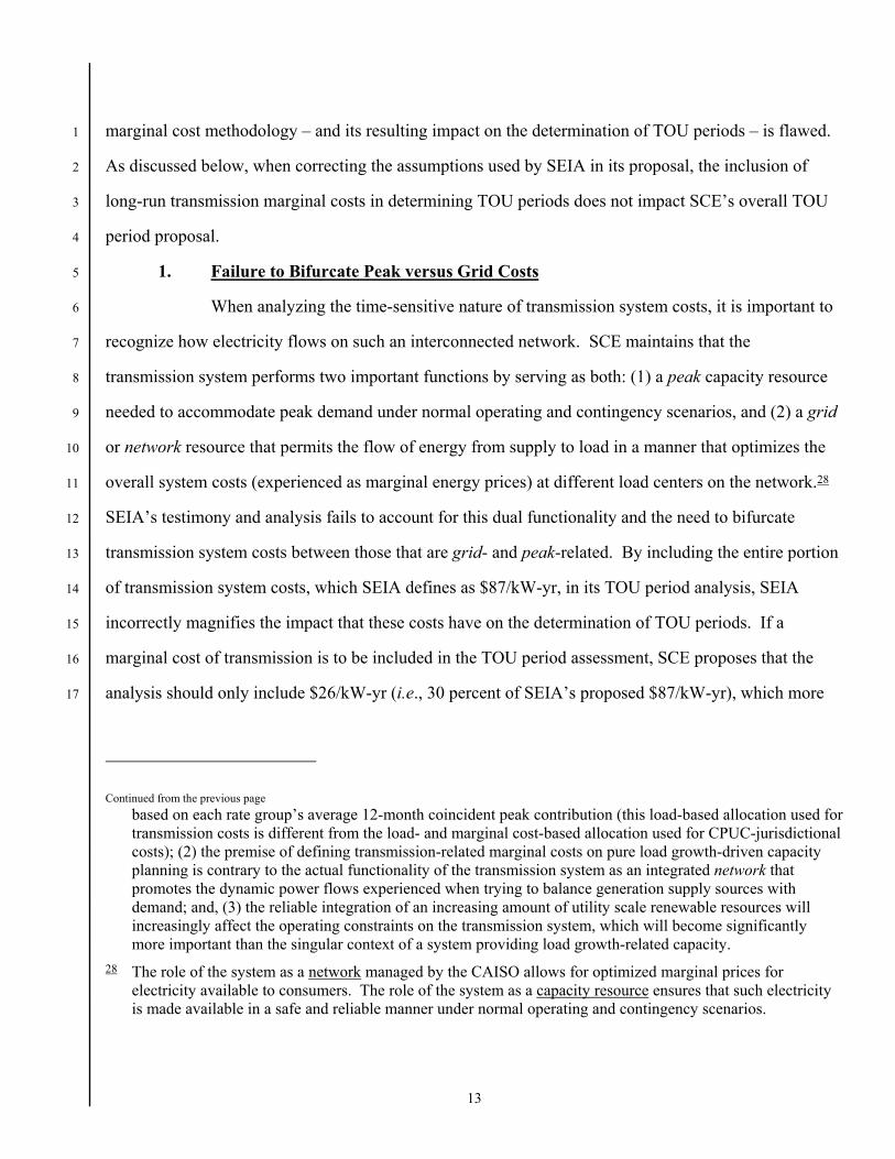
monthly system peak load as the basis for bifurcating transmission system marginal costs between peak 5

and grid. 6

Table III-3 Analysis of Monthly CPs from 2001 to 2015

29 For the purposes of this analysis, SCE suggests using three possible approaches to determine the relevant

portion of transmission system marginal costs that should be functionalized as peak. SCE selected the first method for the purposes of this testimony.

• Use the relative ratio of maximum annual peak load to average 12-CP load (expressed as a percentage) as the basis for functionalizing peak transmission system marginal costs. Based on the past 15 years of 12-CP data, approximately 30 percent of transmission marginal costs are appropriately functionalized as peak.

• Use the relative ratio of maximum annual peak load to minimum annual peak load (expressed as a percentage) as the basis for functionalizing peak transmission system costs. Based on the past 15 years of 12-CP data, approximately 60 percent of transmission marginal costs could be functionalized as peak. SCE does not recommend this approach as average is a better proxy than minimum load levels when determining baseline need on the system.

• Use a FERC accounting-basis such that transmission substation costs are functionalized as peak and the costs associated with transmission lines are functionalized as grid. This method results in approximately 50 percent of transmission system costs being functionalized as peak.

Year January February March April May June July August September October November DecemberAnnual

AverageAnnual

MaxPeak Ratio

(Max/Average-1)2001 13,097 12,466 12,259 13,347 15,355 15,841 16,997 17,610 16,677 16,496 13,050 13,401 14,716 17,610 20%2002 12,755 12,514 12,208 12,631 14,945 16,139 17,820 17,591 18,398 15,445 13,723 13,420 14,799 18,398 24%2003 12,945 12,758 13,403 12,971 17,389 16,633 19,176 19,708 19,983 17,512 13,346 13,818 15,803 19,983 26%2004 13,157 13,109 14,866 17,689 18,572 16,806 19,947 20,358 20,602 15,556 14,073 14,333 16,589 20,602 24%2005 13,743 13,455 13,513 13,504 16,522 16,968 21,599 20,831 18,942 16,685 14,484 14,611 16,238 21,599 33%2006 13,731 13,930 13,433 13,485 16,931 20,947 22,625 20,041 22,166 15,295 15,856 15,202 16,970 22,625 33%2007 14,502 13,832 14,831 14,652 17,230 17,849 20,855 23,130 22,524 16,502 14,910 14,958 17,148 23,130 35%2008 14,583 13,974 13,714 17,093 19,904 21,669 19,403 20,736 20,289 20,451 14,608 15,261 17,641 21,669 23%2009 13,748 13,942 13,237 17,639 16,511 16,720 20,941 21,162 21,792 16,128 13,800 14,436 16,671 21,792 31%2010 13,868 13,675 13,226 12,872 13,562 15,817 21,006 21,259 22,304 17,215 16,124 14,065 16,250 22,304 37%2011 13,668 13,161 14,101 14,276 15,753 16,719 19,721 20,645 22,154 17,901 13,359 14,372 16,319 22,154 36%2012 13,375 13,539 12,943 14,087 16,011 16,182 19,508 21,761 21,187 20,862 14,414 14,185 16,505 21,761 32%2013 14,097 13,271 12,918 13,563 19,194 19,767 20,045 21,226 22,210 14,682 13,697 14,454 16,594 22,210 34%2014 13,268 12,975 12,922 14,740 20,006 17,391 21,126 20,262 22,519 17,641 13,972 13,688 16,709 22,519 35%2015 12,911 13,167 14,783 15,835 15,203 19,071 19,312 22,064 22,557 20,404 13,273 14,050 16,886 22,557 34%

Subtotals 245,838 320,911 31%Monthly Average 13,563 13,318 13,490 14,559 16,873 17,635 20,005 20,559 20,953 17,252 14,179 14,284 16,389

15

Figure III-3 Bifurcation of Transmission System Marginal Costs Between Grid and Peak

Based on Monthly Peak Load

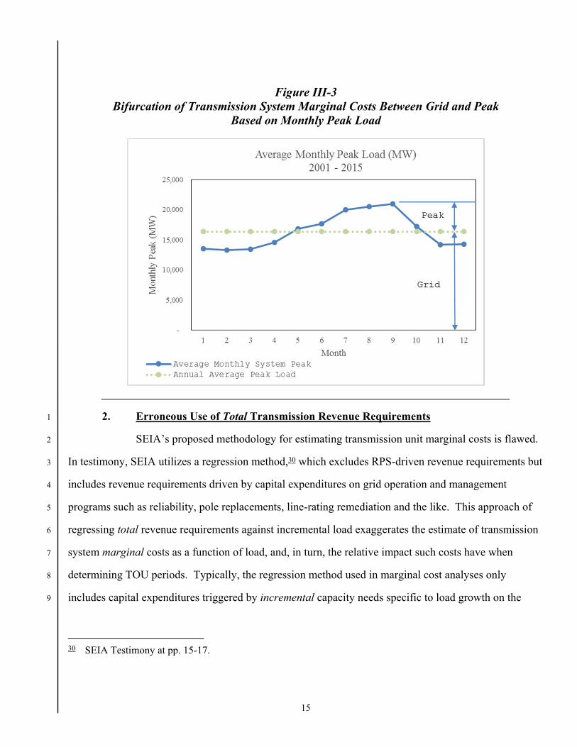
2. Erroneous Use of Total Transmission Revenue Requirements 1

SEIA’s proposed methodology for estimating transmission unit marginal costs is flawed. 2

In testimony, SEIA utilizes a regression method,30 which excludes RPS-driven revenue requirements but 3

includes revenue requirements driven by capital expenditures on grid operation and management 4

programs such as reliability, pole replacements, line-rating remediation and the like. This approach of 5

regressing total revenue requirements against incremental load exaggerates the estimate of transmission 6

system marginal costs as a function of load, and, in turn, the relative impact such costs have when 7

determining TOU periods. Typically, the regression method used in marginal cost analyses only 8

includes capital expenditures triggered by incremental capacity needs specific to load growth on the 9

30 SEIA Testimony at pp. 15-17.

16

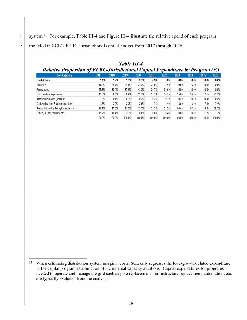
system.31 For example, Table III-4 and Figure III-4 illustrate the relative spend of each program 1

included in SCE’s FERC-jurisdictional capital budget from 2017 through 2026. 2

Table III-4 Relative Proportion of FERC-Jurisdictional Capital Expenditure by Program (%)

31 When estimating distribution system marginal costs, SCE only regresses the load-growth-related expenditure

in the capital program as a function of incremental capacity additions. Capital expenditures for programs needed to operate and manage the grid such as pole replacements, infrastructure replacement, automation, etc. are typically excluded from the analysis.

Cost Category 2017 2018 2019 2020 2021 2022 2023 2024 2025 2026Load Growth 1.4% 1.9% 5.7% 9.3% 0.9% 5.8% 0.0% 0.0% 0.0% 0.0%Reliability 16.9% 24.7% 29.8% 23.2% 25.0% 14.5% 19.6% 15.6% 0.0% 0.0%Renewables 25.3% 38.4% 37.9% 41.2% 29.7% 32.6% 0.0% 0.0% 0.0% 0.0%Infrastructure Replacement 11.0% 9.6% 9.6% 11.2% 11.7% 10.3% 15.6% 16.9% 32.1% 32.1%Transmission Poles (Det+PLP) 1.8% 0.1% 0.1% 0.2% 0.2% 0.1% 0.2% 0.2% 0.4% 0.4%Grid Applications & Communications 1.8% 2.0% 2.2% 2.6% 2.7% 2.4% 3.6% 3.9% 7.4% 7.4%Transmission Line Rating Remediation 26.7% 12.8% 11.9% 11.7% 29.2% 33.9% 60.4% 62.7% 58.9% 58.9%Other (LADWP, Security, etc.) 15.2% 10.4% 2.7% 0.6% 0.6% 0.4% 0.6% 0.6% 1.2% 1.2%

100.0% 100.0% 100.0% 100.0% 100.0% 100.0% 100.0% 100.0% 100.0% 100.0%

17

Figure III-4 Forecast of Transmission System Capital Expenditure ($-Millions) by Program and SCE

System Peak Load (MW)

Load growth spend (blue) is significantly dwarfed by the amount of spend on RPS (gray), 1

reliability (orange) and grid operation needs (all other dotted lines) in the forecast period. Given the 2

relatively insignificant proportion of load growth-driven capital expenditures in the forecast period (i.e., 3

approximately 2-4 percent of the total FERC-jurisdictional spend as shown in Table III-4 above), 4

SEIA’s use of the total transmission revenue requirement (excluding RPS) in the regression model is 5

erroneous and significantly inflates the estimate of transmission system marginal costs. Should the 6

Commission wish to establish a proxy value for transmission system marginal costs, SCE proposes the 7

use of a regression methodology for each asset type, consistent with how such costs are estimated for the 8

subtransmission and distribution system.32 9

32 The regression methodology is similarly used when estimating distribution and subtransmission system

marginal costs. Asset type classification for FERC-jurisdictional transmission assets are lines and (Continued)

18

Further, SEIA attempts to conflate the relationship between the transmission revenue 1

requirement and peak demand to justify using peak demand as the sole cost driver in support of its 2

transmission marginal cost allocation proposal.33 Figure III-5 illustrates the historical trend of the 3

relationship between (1) SCE's annual system peak load, (2) SCE’s annual RPS values, and (3) SCE’s 4

authorized transmission revenue requirement. 5

Figure III-5 Historical Trend of Transmission Revenue Requirement ($-Millions), SCE RPS (%) and

SCE System Peak Load (MW)

The graph indicates that while SCE’s system load growth has increased minimally from 6

2008 through 2016, transmission costs have steadily increased – driven primarily by the State’s RPS 7

Continued from the previous page substations. Should the Commission adopt a similar proxy analysis for FERC-jurisdictional assets, SCE proposes that the cost for lines be functionalized as grid (non-time-variant) and the costs for substations be functionalized as peak (time variant).

33 SEIA Testimony at p. 16, Figure 3.

19

requirements. California’s RPS policy goals require the procurement of renewable energy (not capacity) 1

that is delivered throughout the year. Thus, any discussion of marginal transmission costs must 2

necessarily include some year-round allocation. SEIA’s proposal would allocate 100 percent of the 3

transmission cost to the summer peak period only. FERC’s current 12-CP methodology addresses this 4

by providing a means by which to allocate the transmission functional costs year-round as described in 5

the following section. 6

3. Failure to Consider Established FERC 12-CP Precedent 7

Unlike the CPUC, where marginal cost analyses form the basis of assigning cost 8

responsibility to rate groups,34 FERC has adhered to a CP framework that uses authorized revenue 9

requirements when determining cost responsibility. The basic premise of the CP method is that monthly 10

system peaks are the primary determinant for when facilities are employed, and, therefore, system 11

demand coincident with such peaks results in an equitable allocation of system costs. FERC’s use of the 12

12-CP methodology allows for the reasonable accommodation of the seasonal supply and demand 13

constraints across all months of the year. 14

While SCE maintains that transmission cost allocation is more appropriately vetted in 15

FERC rate proceedings, the cost analysis presented here uses 12-CP as the basis for illustrating how the 16

time-sensitive nature of transmission system costs could inform the determination of TOU periods. The 17

heat map in Figure III-6 illustrates the allocation of peak capacity-related transmission system costs 18

using the 12-CP framework. 19

34 D.92749.

20

Figure III-6 2024 Transmission System Costs Based on 12-CP ($/kW-hr)

The capacity-related portion of transmission system marginal costs were allocated to each 1

month based on the relative proportion of monthly peak load estimated for the year 2024. To arrive at 2

an hourly allocation of costs, this monthly allocation was then equally prorated to the top-20 peak load 3

hours of each month. This analysis indicates that more peak “weight” should be given to the 4 to 9 p.m. 4

period, but SCE defers to the Commission in future ratesetting proceedings as to whether transmission 5

system cost recovery should be included in TOU period analysis. 6

4. Failure to Include the Impacts of Distributed Generation (DG) and Diversity 7

When applying the peak capacity allocation factor (PCAF) methodology to determine the 8

time-sensitive nature of peak-capacity-related transmission system costs, SEIA erroneously uses 9

historical SCE system load at the CAISO-system level, which excludes behind-the-meter (BTM) solar 10

Year Month 1 2 3 4 5 6 7 8 9 10 11 12 13 14 15 16 17 18 19 20 21 22 23 24 Total1 -$ -$ -$ -$ -$ -$ -$ -$ -$ -$ -$ -$ -$ -$ -$ -$ -$ 0.19$ 1.41$ 0.28$ -$ -$ -$ -$ 1.9$ 2 -$ -$ -$ -$ -$ -$ -$ -$ -$ -$ -$ -$ -$ -$ -$ -$ -$ -$ 1.04$ 0.70$ -$ -$ -$ -$ 1.7$ 3 -$ -$ -$ -$ -$ -$ -$ -$ -$ -$ -$ -$ -$ -$ -$ -$ -$ -$ 0.13$ 0.44$ 0.57$ 0.63$ -$ -$ 1.8$ 4 -$ -$ -$ -$ -$ -$ -$ -$ -$ -$ -$ -$ -$ -$ -$ -$ -$ -$ -$ -$ 0.72$ 1.09$ -$ -$ 1.8$ 5 -$ -$ -$ -$ -$ -$ -$ -$ -$ -$ -$ -$ -$ -$ -$ -$ -$ -$ 0.30$ 0.20$ 0.49$ 0.69$ 0.30$ -$ 2.0$ 6 -$ -$ -$ -$ -$ -$ -$ -$ -$ -$ -$ -$ -$ -$ -$ -$ -$ 0.33$ 0.67$ 0.33$ 0.22$ 0.67$ -$ -$ 2.2$ 7 -$ -$ -$ -$ -$ -$ -$ -$ -$ -$ -$ -$ -$ -$ -$ -$ 0.13$ 0.78$ 1.17$ 0.26$ 0.13$ 0.13$ -$ -$ 2.6$ 8 -$ -$ -$ -$ -$ -$ -$ -$ -$ -$ -$ -$ -$ -$ -$ 0.31$ 0.46$ 0.93$ 0.62$ 0.31$ 0.31$ 0.16$ -$ -$ 3.1$ 9 -$ -$ -$ -$ -$ -$ -$ -$ -$ -$ -$ -$ -$ -$ -$ -$ 0.25$ 0.63$ 0.50$ 0.50$ 0.50$ 0.13$ -$ -$ 2.5$

10 -$ -$ -$ -$ -$ -$ -$ -$ -$ -$ -$ -$ -$ -$ -$ -$ -$ 0.40$ 0.50$ 0.90$ 0.20$ -$ -$ -$ 2.0$ 11 -$ -$ -$ -$ -$ -$ -$ -$ -$ -$ -$ -$ -$ -$ -$ -$ -$ 0.70$ 1.08$ 0.06$ -$ -$ -$ -$ 1.8$ 12 -$ -$ -$ -$ -$ -$ -$ -$ -$ -$ -$ -$ -$ -$ -$ -$ -$ 0.58$ 0.88$ 0.49$ -$ -$ -$ -$ 1.9$

Total -$ -$ -$ -$ -$ -$ -$ -$ -$ -$ -$ -$ -$ -$ -$ 0.31$ 0.84$ 4.53$ 8.28$ 4.46$ 3.14$ 3.48$ 0.30$ -$ 25.3$

1 -$ -$ -$ -$ -$ -$ -$ -$ -$ -$ -$ -$ -$ -$ -$ -$ -$ -$ -$ -$ -$ -$ -$ -$ -$ 2 -$ -$ -$ -$ -$ -$ -$ -$ -$ -$ -$ -$ -$ -$ -$ -$ -$ -$ -$ -$ -$ -$ -$ -$ -$ 3 -$ -$ -$ -$ -$ -$ -$ -$ -$ -$ -$ -$ -$ -$ -$ -$ -$ -$ -$ -$ -$ -$ -$ -$ -$ 4 -$ -$ -$ -$ -$ -$ -$ -$ -$ -$ -$ -$ -$ -$ -$ -$ -$ -$ -$ -$ -$ -$ -$ -$ -$ 5 -$ -$ -$ -$ -$ -$ -$ -$ -$ -$ -$ -$ -$ -$ -$ -$ -$ -$ -$ -$ -$ -$ -$ -$ -$ 6 -$ -$ -$ -$ -$ -$ -$ -$ -$ -$ -$ -$ -$ -$ -$ -$ -$ -$ -$ -$ -$ -$ -$ -$ -$ 7 -$ -$ -$ -$ -$ -$ -$ -$ -$ -$ -$ -$ -$ -$ -$ -$ -$ -$ -$ -$ -$ -$ -$ -$ -$ 8 -$ -$ -$ -$ -$ -$ -$ -$ -$ -$ -$ -$ -$ -$ -$ -$ -$ -$ -$ -$ -$ -$ -$ -$ -$ 9 -$ -$ -$ -$ -$ -$ -$ -$ -$ -$ -$ -$ -$ -$ -$ -$ -$ -$ -$ -$ -$ -$ -$ -$ -$

10 -$ -$ -$ -$ -$ -$ -$ -$ -$ -$ -$ -$ -$ -$ -$ -$ -$ -$ -$ -$ -$ -$ -$ -$ -$ 11 -$ -$ -$ -$ -$ -$ -$ -$ -$ -$ -$ -$ -$ -$ -$ -$ -$ -$ -$ -$ -$ -$ -$ -$ -$ 12 -$ -$ -$ -$ -$ -$ -$ -$ -$ -$ -$ -$ -$ -$ -$ -$ -$ -$ -$ -$ -$ -$ -$ -$ -$

Total -$ -$ -$ -$ -$ -$ -$ -$ -$ -$ -$ -$ -$ -$ -$ -$ -$ -$ -$ -$ -$ -$ -$ -$ -$

Weekday

2024

2024

Weekend

21

and other DG resources.35 Load profiles, and in turn transmission system marginal costs, should 1

reasonably include estimates of DG in the modeled test year (i.e., like the CAISO’s “net” load curve 2

does for purposes of the balance of this proceeding). BTM DG is becoming an increasingly important 3

part of the energy mix in California and including the time-sensitive impact such resources have on 4

SCE’s load shape is critical in identifying the time-sensitive nature of transmission and distribution 5

system peaks. Much like solar RPS, solar DG has the similar effect of exacerbating the duck curve, with 6

an additional impact of reducing overall demand on the system by the amount of energy customers self-7

supply for their onsite needs. The California Energy Commission’s (CEC) 2016 Integrated Energy 8

Policy Report (IEPR) demonstrates that DG is an important consideration in system planning for both 9

energy and capacity needs, and includes a range of estimates of DG penetration for each demand 10

scenario modeled.36 As such, any assessment of transmission marginal costs must include the forward-11

looking impacts of DG, which SEIA failed to do in its analysis.37 When DG is considered, the CEC 12

estimates that peak transmission loads shift to later in the day (HE18 by 2024). 13

SEIA’s use of the PCAF methodology to estimate transmission system marginal costs 14

also ignores the impacts of diversity. As the transmission system integrates an increasing number of 15

renewable supply sources on the grid, the expected supply and load diversity across the transmission 16

system network should be appropriately accounted for when analyzing time-variant transmission 17

constraints and costs.38 Including the effect of such diversity is crucial to assessing how time-sensitive 18

35 Though admittedly, SEIA’s testimony at p. 16, fn 31 is confusing as it references unknown SCE material

sponsored by a Pacific Gas and Electric Company (PG&E) employee.

36 Expected trends related to self-generation, including solar BTM DG for SCE’s planning area, are available in CEC Docket 16-IEPR-05. See also Chapter 4 – Peak Shift Scenario Analysis in Garcia, Cary and Chris Kavalec. 2017. California Energy Demand Updated Forecast, 2017-2027. California Energy Commission. Publication Number: CEC-200-2016-016.

37 SEIA’s analysis is all generally backward-looking, which is not consistent with Policy Guideline #4 of D.17-01-006.

38 In compliance with California policy objectives, as more renewable sources integrate with the system, consideration should be given to the time-sensitive nature with which both load and supply constraints effect the planning and design of the transmission system.

22

constraints on the system affect costs at different load and supply hubs on the transmission system.39 1

SEIA’s analysis, which uses SCE’s CAISO-level load, ignores how load and supply diversity across the 2

network impacts capacity-related costs. This gap is visible in the heat maps shown below (Figures III-7 3

and III-8), which illustrate the diversity in peak loads for two transmission substations. 4

Figure III-7 Average Load (MW) by Hour for Vincent Substation AA Bank

Figure III-8 Average Load (MW) by Hour for Windhub Substation AA Bank

5. Conclusion 5

In summary, SCE does not agree with SEIA’s use of the following assumptions when 6

analyzing transmission system marginal costs and their resulting impact on the determination of TOU 7

39 A transmission substation (AA Bank) such as Windhub affects system constraints very differently when

compared with Vincent substation. Using CAISO-level load does not account for such diversity. In the past, generation-following load allowed for a load-based model when determining system constraints and, therefore, costs. However, as more renewables integrate with the transmission system, generation is not necessarily load following. Analyzing the implications of both demand (load) and supply is critical when assessing the time-sensitive nature of transmission system marginal costs.

Year Average LoadMonth 1 2 3 4 5 6 7 8 9 10 11 12 13 14 15 16 17 18 19 20 21 22 23 24

1 1,217 1,162 1,114 1,082 1,074 1,126 1,199 1,229 1,243 1,321 1,346 1,378 1,381 1,384 1,382 1,380 1,373 1,335 1,398 1,394 1,406 1,390 1,336 1,286 2 1,151 1,063 1,027 1,001 993 1,050 1,147 1,108 1,168 1,266 1,336 1,394 1,439 1,453 1,462 1,471 1,459 1,419 1,477 1,464 1,413 1,366 1,303 1,217 3 1,052 998 949 925 917 954 1,048 1,093 1,121 1,234 1,337 1,428 1,448 1,476 1,507 1,528 1,531 1,497 1,453 1,445 1,444 1,380 1,255 1,151 4 1,108 1,070 1,009 970 976 1,007 1,094 1,177 1,290 1,420 1,538 1,600 1,651 1,670 1,682 1,675 1,668 1,615 1,518 1,425 1,497 1,434 1,328 1,197 5 1,261 1,188 1,107 1,076 1,074 1,105 1,166 1,289 1,435 1,590 1,696 1,737 1,774 1,787 1,803 1,813 1,831 1,794 1,749 1,661 1,742 1,672 1,531 1,368 6 1,108 1,085 1,028 1,000 981 983 1,022 1,137 1,287 1,425 1,544 1,602 1,655 1,666 1,681 1,680 1,678 1,637 1,542 1,360 1,299 1,305 1,212 1,143 7 1,218 1,171 1,144 1,077 1,042 1,051 1,074 1,155 1,321 1,424 1,549 1,637 1,717 1,814 1,840 1,850 1,868 1,809 1,716 1,488 1,434 1,417 1,369 1,311 8 1,387 1,304 1,249 1,201 1,156 1,176 1,192 1,232 1,418 1,573 1,740 1,895 2,009 2,082 2,093 2,122 2,112 2,038 1,891 1,668 1,679 1,680 1,646 1,517 9 1,368 1,279 1,201 1,134 1,085 1,118 1,174 1,173 1,354 1,538 1,697 1,851 1,974 2,081 2,147 2,183 2,160 2,069 1,840 1,739 1,725 1,729 1,620 1,492

10 1,286 1,191 1,118 1,054 1,031 1,067 1,166 1,211 1,280 1,458 1,617 1,733 1,810 1,886 1,910 1,946 1,936 1,836 1,672 1,638 1,648 1,628 1,560 1,436 11 1,313 1,270 1,195 1,132 1,126 1,207 1,286 1,241 1,326 1,401 1,462 1,549 1,567 1,597 1,632 1,628 1,559 1,580 1,619 1,600 1,609 1,554 1,472 1,405 12 1,480 1,450 1,382 1,333 1,339 1,422 1,564 1,571 1,592 1,637 1,638 1,642 1,624 1,599 1,652 1,665 1,632 1,711 1,774 1,785 1,776 1,748 1,716 1,651

VINCENT AA BANK (LOAD)

2015

Year Average LoadMonth 1 2 3 4 5 6 7 8 9 10 11 12 13 14 15 16 17 18 19 20 21 22 23 24

1 84 67 65 62 57 60 71 77 70 50 54 68 92 136 145 152 151 164 164 154 143 135 114 105 2 340 310 299 294 300 313 298 265 233 224 227 235 288 352 382 387 410 422 411 434 426 384 351 328 3 559 604 569 575 521 473 435 367 313 337 353 402 431 425 431 457 479 536 576 595 591 579 591 589 4 744 733 728 676 626 591 546 479 503 459 432 421 457 509 544 556 642 737 808 764 768 762 756 746 5 882 893 836 823 785 726 664 604 550 480 458 493 543 593 669 788 910 971 1,004 963 845 919 955 949 6 1,079 1,048 1,030 999 908 848 804 730 629 541 519 500 534 600 723 851 964 989 1,056 1,079 1,070 1,091 1,089 1,073 7 780 778 755 695 602 531 440 371 367 310 251 245 275 304 381 470 556 673 736 745 727 767 788 764 8 991 965 931 908 812 727 645 548 472 398 327 333 371 430 523 652 779 878 942 938 1,000 1,087 1,072 1,049 9 425 395 386 366 320 285 271 250 230 217 219 213 253 292 359 431 471 512 495 496 562 536 464 424

10 441 428 382 367 331 303 261 244 234 235 262 296 264 280 296 344 380 420 384 438 445 433 422 471 11 311 394 362 324 302 237 214 218 254 290 356 425 476 455 474 457 447 490 428 429 381 348 328 316 12 607 610 556 481 486 486 486 500 494 544 529 551 610 630 664 627 576 561 590 640 649 656 692 643

WINDHUB AA-BANK

2015

23

periods: (1) SEIA’s inclusion of the entire portion of transmission system marginal costs ($87/ kW-yr) 1

and total revenue requirements – only a portion of these costs are peak-capacity-related and only those 2

costs should be used when analyzing the time-sensitive nature of transmission system marginal costs;40 3

(2) the PCAF method applied to CAISO system level-load with a resulting summer-only allocation of 4

cost – this method fails to account for both the diversity of system constraints and the judicious 5

application of the CP framework adopted by the FERC when requiring that costs be allocated to all 6

twelve months of the year; and, (3) SEIA’s use of SCE’s forecast of delivered loads that exclude BTM 7

solar and other DG resources – load profiles, and in turn transmission system marginal costs, should 8

reasonably include estimates of DG in the modeled test year. 41 9

When correcting for these items, SCE found that the inclusion of transmission system 10

marginal costs ($26/kW-yr) in the determination of TOU periods does not materially impact SCE’s 11

original TOU period proposal, as shown in Figures III-9 through III-12. 12

40 Again, SCE proposes that only 30 percent of SEIA’s estimate of transmission system marginal costs are peak-

related. The balance of costs are grid-related (and not time-dependent), and should therefore be excluded from the analysis of how transmission system marginal costs impact the determination of TOU periods

41 As discussed in Exhibit SCE-1 and Chapter II.D, SCE’s use of 2024 as the modeled test year when setting TOU periods is appropriate as it ensures that updated TOU periods maintain viability over a sufficiently stable duration of time.

24

Figure III-9 2024 Average Total Marginal Cost including Transmission ($/kWh-hr) –

Summer Weekday


Winter Weekday

25


Summer Weekend

26


Winter Weekend

B. Seasonal Definitions 1

In testimony, SEIA opposes SCE’s proposal to maintain a four-month summer season (June – 2

September), and argues instead that SCE should move to a six-month summer (May – October) – 3

consistent with the positions SEIA has taken in the pending PG&E and San Diego Gas & Electric 4

Company (SDG&E) Phase 2 cases.42 SEIA argues that climate data shows that the summer season is 5

becoming longer, not shorter, in southern California, with an increasing trend of very hot days in May 6

and October that drive electric demand.43 In response to SEIA’s arguments, SCE presents data below 7

that further justifies a four-month summer season comprised of the months June through September, and 8

an eight-month winter season comprised of the months October through May. 9

42 A proposed decision in SDG&E’s Phase 2 proceeding (A.15-04-012) issued on May 18, 2017 declined to

adopt SEIA’s proposal to move May into the summer season (see Proposed Decision Adopting Revenue Allocation and Rate Design for San Diego Gas & Electric Company at p. 17.). PG&E, in its current GRC Phase 2 proceeding, is also advocating for a four-month summer consistent with what SCE has proposed herein (see A.16-06-013, Exhibit (PG&E-2) Volume 1 at p. 12-9).

43 SEIA Testimony at p. iii.

27

1. Marginal Cost Analysis 1

As described in Exhibit SCE-1, an overarching goal when defining seasons and TOU 2

period is to group together hours with similar costs and, at the same time, obtain reasonable separation 3

in costs between TOU periods.44 As such, SCE defines the summer season to include the months of 4

June through September on the basis of an analysis of marginal costs, which shows that the highest costs 5

are distributed mainly in the months of June through September in SCE’s proposed peak period (see 6

Table III-5 and Figure III-13). 7

Table III-5 Average Marginal Costs for HE17 – HE21 ($/kWh)


Month Weekend WeekdayJanuary 0.0703 0.0811February 0.0688 0.0798March 0.0634 0.0768April 0.0567 0.0707May 0.0568 0.0723June 0.0641 0.1003July 0.0770 0.1107August 0.0921 0.1709September 0.1628 0.4319October 0.0760 0.0899November 0.0759 0.0877December 0.0788 0.0928

Day TypeAverage Marginal Cost for HE17-HE21($/kWh)

28

Figure III-13 Average Marginal Costs for HE17 – HE21 ($/kWh)

The costs for May and October are more similar to those of the other winter months, 1

which is why SCE appropriately included these months in the winter season instead of the summer 2

season. In fact, May is a less expensive month on both weekdays and weekends than November, 3

December, January, February, and March. 4

2. Use of Actual Load Data as Opposed to Maximum Daily Temperature Proxy 5

In testimony, SEIA asserts that the climate is changing and the summer season is 6

becoming longer in southern California “with an increasing trend of very hot days in May and October 7

that drive electric demand.”45 To support this argument, SEIA provides an analysis correlating 2014 8

daily maximum temperatures with SCE’s system load data to show that system load is highly correlated 9

with temperature.46 While SCE does not disagree, it is important to note that a singular peak day 10

temperature is not the only cause of increased load. As stated in the publication Electric Power 11

45 SEIA Testimony at p. iii.

46 Id. at Figure 7.

29

Distribution Reliability, “[m]aximum temperature is only one of the four weather factors that 1

significantly impact electric load. The other three are humidity, solar illumination, and the number of 2

consecutive extreme days…[c]onsecutive extreme days further increases loads since (1) the thermal 3

inertia of buildings will cause them to slowly increase in temperature over several days, and (2) many 4

people will not utilize air conditioning until it has been uncomfortably hot for several days.”47 In other 5

words, an isolated, anomalous hot day in May does not significantly drive electric load compared to an 6

extended heat storm in late July. Also, customers tend to utilize air conditioning more often when it is 7

traditionally expected to be hot (e.g., mid-summer) compared to when it is hot in a more unseasonable 8

time (e.g., April or May). The factors mentioned above help explain why the first day in May that 9

reaches 95 degrees does not create as much demand for electricity used for cooling compared to the 10

third day of a heat storm in July where the maximum temperature also reaches 95 degrees. 11

To validate these assertions, SCE performed an analysis on actual historical system load 12

data rather than relying on daily maximum temperature as a proxy, which SEIA has done. Table III-6 13

shows the distribution of the annual highest 100 peak days for both SCE and CAISO loads in the most 14

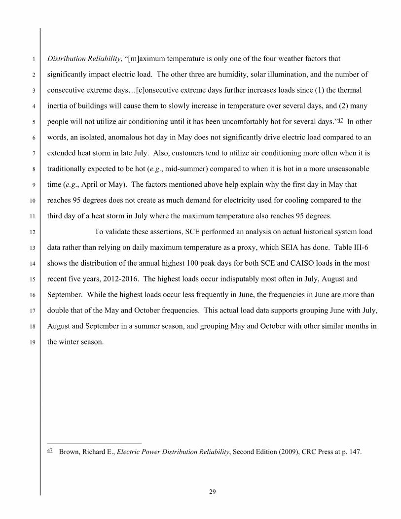
recent five years, 2012-2016. The highest loads occur indisputably most often in July, August and 15

September. While the highest loads occur less frequently in June, the frequencies in June are more than 16

double that of the May and October frequencies. This actual load data supports grouping June with July, 17

August and September in a summer season, and grouping May and October with other similar months in 18

the winter season. 19

47 Brown, Richard E., Electric Power Distribution Reliability, Second Edition (2009), CRC Press at p. 147.

30

Table III-6 Distribution of CAISO and SCE Top 100 Annual Load Peak Days for 2012-2016

C. Determination of Peak-Related Marginal Distribution Costs (PLRF Methodology) 1

As explained in Exhibit SCE-1, once design demand distributional marginal costs have been split 2

between those that peak-driven and those that are grid-related, SCE employs a peak load risk factor 3

(PLRF) methodology to determine hourly allocation.48 The PLRF methodology uses triggers defined by 4

distribution planners to identify specific capacity needs, also known as planning thresholds, to allocate 5

peak-driven capacity costs to each hour of the year. In testimony, SEIA presents four arguments for 6

why the PLRF methodology fails to yield a reasonable allocation of marginal distribution costs, which 7

then impacts the determination of TOU periods.49 SCE rebuts the four arguments made by SEIA related 8

to the PLRF methodology, as follows. 9

1. Issue 1 – Siting of DG 10

SEIA’s first issue with SCE’s proposed PLRF methodology is the assumption that future 11

DG will be sited in the same location as existing DG, since the Commission’s Distribution Resource 12

Planning (DRP) initiative is to encourage DG to be located where it can provide the most benefits to the 13

system (which could result in significant changes to past patterns of DG deployment).50 While SCE 14


49 SEIA Testimony at p. 22.

50 Id.

Month Frequency Percent Frequency PercentApril 2 0.4%May 16 3.2% 21 4.2%June 81 16.2% 65 13.0%July 131 26.2% 124 24.8%August 138 27.6% 142 28.4%September 113 22.6% 116 23.2%October 20 4.0% 29 5.8%November 0 0.0% 1 0.2%December 1 0.2%

CAISO SCE

31

does not dispute that future locational trends in DG penetration may change, SCE’s initial analysis 1

assumed that the future siting of DG will continue to remain generally consistent with current patterns. 2

SCE’s analysis is based on the assumption that the economics and site-specific drivers of DG 3

penetration observed on different distribution circuits would tend to generally continue in the forecast 4

period. In SCE’s analysis, the majority of circuits (approximately 82 percent) have existing DG 5

customers. Table III-7 shows the distribution of the percent of circuits with and without DG customers 6

in SCE’s eight planning regions. 7

Table III-7 DG Circuit Penetration by Planning Region (%)

Planning

Regions

Percent of Circuits With Existing DG Customers

Percent of Circuits Without Existing DG Customers

Desert 10.4% 2.8%

Metro East 16.1% 2.5%

Metro West 17.5% 4.8%

North Coast 10.2% 1.4%

Orange 13.2% 2.6%

Rurals 4.1% 1.9%

San Jacinto 5.5% 1.0%

San Joaquin 4.8% 1.3%

Total 81.7% 18.3%

SEIA criticizes SCE’s methodology without providing an alternative in regards to DG 8

siting. SCE offers the following additional analysis in an effort to ascertain the impact of the 2020 zero 9

net energy (ZNE) housing requirements. Figure III-14 presents the effect of DG on future grid 10

conditions by comparing the aggregated load profiles of a recently-completed residential development 11

consisting of homes both with and without DG systems. 12

32

Figure III-14 Average Hourly Load Profiles for Residential Development with DG and Non-DG

Customers

The data used in this analysis was comprised of homes all built in the same year with the 1

average home size (in terms of square footage) consistent across both DG and non-DG groups, therefore 2

allowing the non-DG customers to represent a viable control group. This control group allows SCE to 3

estimate the behavior of DG customers if they had not installed DG. The blue line (DG KWH_DEL) on 4

the graph shows the average load profile for customers that have DG and represents hourly load that is 5

delivered from SCE to the customer. The red line (DG KWH_REC) is the surplus DG energy that these 6

customers send back to SCE’s system after serving the on-site consumption. The green line (NON-DG) 7

shows the profile of customers in the same housing development that do not have DG systems. All load 8

0

0.5

1

1.5

2

2.5

1 2 3 4 5 6 7 8 9 10 11 12 13 14 15 16 17 18 19 20 21 22 23 24

kW

Hour Ending (PST)

SUMMER WORKDAYS

DG KWH_DEL

DG KWH_REC

NON-DG

Non-DGPeak @ Hour 17

DG Peak @ Hour 19

33

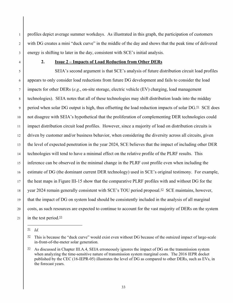
profiles depict average summer workdays. As illustrated in this graph, the participation of customers 1

with DG creates a mini “duck curve” in the middle of the day and shows that the peak time of delivered 2

energy is shifting to later in the day, consistent with SCE’s initial analysis. 3

2. Issue 2 – Impacts of Load Reduction from Other DERs 4

SEIA’s second argument is that SCE’s analysis of future distribution circuit load profiles 5

appears to only consider load reductions from future DG development and fails to consider the load 6

impacts for other DERs (e.g., on-site storage, electric vehicle (EV) charging, load management 7

technologies). SEIA notes that all of these technologies may shift distribution loads into the midday 8

period when solar DG output is high, thus offsetting the load reduction impacts of solar DG.51 SCE does 9

not disagree with SEIA’s hypothetical that the proliferation of complementing DER technologies could 10

impact distribution circuit load profiles. However, since a majority of load on distribution circuits is 11

driven by customer and/or business behavior, when considering the diversity across all circuits, given 12

the level of expected penetration in the year 2024, SCE believes that the impact of including other DER 13

technologies will tend to have a minimal effect on the relative profile of the PLRF results. This 14

inference can be observed in the minimal change in the PLRF cost profile even when including the 15

estimate of DG (the dominant current DER technology) used in SCE’s original testimony. For example, 16

the heat maps in Figure III-15 show that the comparative PLRF profiles with and without DG for the 17

year 2024 remain generally consistent with SCE’s TOU period proposal.52 SCE maintains, however, 18

that the impact of DG on system load should be consistently included in the analysis of all marginal 19

costs, as such resources are expected to continue to account for the vast majority of DERs on the system 20

in the test period.53 21

51 Id.

52 This is because the “duck curve” would exist even without DG because of the outsized impact of large-scale in-front-of-the-meter solar generation.

53 As discussed in Chapter III.A.4, SEIA erroneously ignores the impact of DG on the transmission system when analyzing the time-sensitive nature of transmission system marginal costs. The 2016 IEPR docket published by the CEC (16-IEPR-05) illustrates the level of DG as compared to other DERs, such as EVs, in the forecast years.

34

Figure III-15 2024 Circuit Weekday PLRFs (%) With and Without DG54

3. Issue 3 – Hourly Allocation 1

SEIA’s third issue with SCE’s proposed PLRF methodology is that it uses an hourly 2

allocation based on the sum across all distribution circuits of loads that exceed 73 percent of a planning 3

threshold trigger capacity for each circuit, and then does not weight the allocation by the amount by 4

which the 73 percent threshold is exceeded. SEIA contends that a PCAF allocation should be used 5

instead, whereby the hours that exceeded the threshold would then be weighted based on the amount by 6

which they exceeded the threshold.55 7

SEIA’s statement that, in the PLRF methodology, “the hours with loads near 100 percent 8

of planning capacity are not assigned a much higher weight than loads that are just above the 73 percent 9

54 These heat maps illustrate only a single cost driver to inform the discussion on the impact of future DERs on

distribution circuits, and are not reflective of the relative weighting of all costs that inform the development of TOU periods.


35

trigger” is erroneous.56 In fact, the PLRF methodology considers the magnitude of the peak load as the 1

weight of the allocation.57 This point is illustrated by the following example and the data presented in 2

Table III-8 and Figure III-16. 3

56 Id.

57 The peak capacity constraint of a resource should be based on the relationship between peak load and the planning criteria used by system planners (planned loading limit or PLL). The PLRF approach uses such a relationship when identifying the potential of time-sensitive capacity constraints that may be experienced by the resource.

36

Table III-8 PLRF Weighted Allocation Example

For simplicity, assume that the entire system consists of one circuit and the entire year is 1

reduced to 24 hours (Column A). The capacity of this circuit is 180 MW (Column C). At 73 percent of 2

capacity, the threshold is 131 MW (Column D). Any loads exceeding 131 MW are considered peak 3

load (Column E). The PLRF (Column F) is calculated as the ratio of the peak load at hour x over the 4

sum of the peak loads. At hour 18, the peak load is at 100 percent capacity, and has a PLRF value of 8.5 5

percent; whereas at hour 17, the peak load is only slightly higher than the 73 threshold, so it has a lower 6

PLRF value of 6.4 percent. Hence, the magnitude of the peak load is given proportionate weight in 7

SCE’s proposed PLRF methodology. 8

37

Figure III-16 PLRF Weighted Allocation Example Results

4. Issue 4 – Use of 2024 PLRFs 1

SEIA’s last issue with SCE’s proposed PLRF methodology is that SCE used 2024 PLRFs 2

in the tool developed for the analysis of 2021 hourly marginal costs. SEIA argues that SCE should have 3

developed 2021 PLRFs based on projected distribution loads and DG forecasts for 2021.58 4

SCE agrees with SEIA that the PLRFs submitted in the RDW tool supporting Exhibit 5

SCE-1 were only derived for the year 2024.59 For purposes of this rebuttal, and in acknowledgement of 6

SEIA’s observation, SCE developed separate PLRFs for the year 2021. In Figure III-17, SCE presents a 7

comparison of the 2021 and 2024 weekday PLRF heat maps. The 2021 PLRFs are generally consistent 8

with the PLRFs for the year 2024 originally submitted in Exhibit SCE-1. 9


59 The PLRFs included for the year 2021 were the same as 2024 but mapped by season and day type to the year 2021.

38

Figure III-17 2021 and 2024 Circuit PLRF Weighted Allocation Results with DG

D. Marginal Generation Flex Capacity Costs – Ramp Allocation 1

When performing its TOU period analysis, SEIA allocated marginal generation capacity ramping 2

costs (also referred to as “flex”) to four hours of the ramp and not just the ending hours of the ramp as 3

SCE proposed.60 As more fully explained in Exhibit SCE-1, SCE’s proposal to allocate the cost of flex 4

capacity to only the latter two hours of the ramp reflects the fact that the capacity constraint becomes 5

more pronounced in the latter hours as opposed to the first hour.61 SEIA’s proposal of using four hours 6

is also in direct conflict with the established criteria used by the Commission and the CAISO when 7

defining the ramp constraint as the maximum three-hour ramp.62 8

Appropriately-set TOU periods allow the Load-Serving Entity to convey a retail price signal so 9

that customers can modify their consumption behavior in a manner that reduces their impact on cost. As 10



62 Id., fn 42.

39

such, it is important to recognize that the effect of the ramp can be mitigated by either raising the belly 1

or lowering the head of the duck (see Figure III-18). In the winter season, when there is an increased 2

tendency to experience significant ramps, peak capacity need on the system is relatively insignificant.63 3

Further, the end of the maximum three-hour ramp tends to coincide with the maximum peak in the day. 4

Excluding the capacity allocation in the first hour, and aligning most of the capacity closest to the peak, 5

simultaneously achieves two objective: first, it mitigates the capacity signal in the hour closest to the 6

belly of the duck, therefore allowing customers to modify consumption in a manner that raises the belly 7

of the duck; and, second, it inflates the price signal in the hour closest to the peak hour, therefore 8

allowing customers to modify consumption in a manner that lowers the head of the duck. 9

SCE’s proposal to allocate 70 percent of the flex costs in the third hour of the ramp and 30 10

percent in the second hour is based on the proportionate magnitude of ramp in each hour, with a 11

subsequent adjustment that moves the flex capacity cost allocation of the first hour to the third hour. 12

This works to accomplish both objectives described above, and as shown in Figure III-18. 13

63 This observation is supported by the relatively insignificant values of peak LOLEs in winter months.

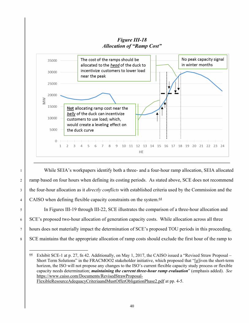
40

Figure III-18 Allocation of “Ramp Cost”

While SEIA’s workpapers identify both a three- and a four-hour ramp allocation, SEIA allocated 1

ramp based on four hours when defining its costing periods. As stated above, SCE does not recommend 2

the four-hour allocation as it directly conflicts with established criteria used by the Commission and the 3

CAISO when defining flexible capacity constraints on the system.64 4

In Figures III-19 through III-22, SCE illustrates the comparison of a three-hour allocation and 5

SCE’s proposed two-hour allocation of generation capacity costs. While allocation across all three 6

hours does not materially impact the determination of SCE’s proposed TOU periods in this proceeding, 7

SCE maintains that the appropriate allocation of ramp costs should exclude the first hour of the ramp to 8

64 Exhibit SCE-1 at p. 27, fn 42. Additionally, on May 1, 2017, the CAISO issued a “Revised Straw Proposal –

Short Term Solutions” in the FRACMOO2 stakeholder initiative, which proposed that “[g]iven the short-term horizon, the ISO will not propose any changes to the ISO’s current flexible capacity study process or flexible capacity needs determination; maintaining the current three-hour ramp evaluation” (emphasis added). See https://www.caiso.com/Documents/RevisedStrawProposal-FlexibleResourceAdequacyCriteriaandMustOfferObligationPhase2.pdf at pp. 4-5.

41

allow for more accurate price signals that incent customers to behave in a way that best mitigates the 1

issues associated with both the belly and the head of the duck curve. 2

Figure III-19 2021 Marginal Generation Capacity Costs ($/kW-hr) with Two-Hour Flex Allocation

Figure III-20 2021 Marginal Generation Capacity Costs ($/kW-hr) with Three-Hour Flex Allocation

Year Month 1 2 3 4 5 6 7 8 9 10 11 12 13 14 15 16 17 18 19 20 21 22 23 24 Total1 -$ -$ -$ -$ -$ -$ 0.08$ 0.18$ -$ -$ -$ -$ -$ -$ -$ 0.03$ 0.22$ 0.64$ 0.66$ -$ -$ -$ -$ -$ 1.80$ 2 -$ -$ -$ -$ -$ -$ 0.04$ 0.09$ -$ -$ -$ -$ -$ -$ -$ -$ 0.06$ 0.64$ 1.15$ -$ -$ -$ -$ -$ 1.99$ 3 -$ -$ -$ -$ -$ -$ -$ -$ -$ -$ -$ -$ -$ -$ -$ -$ 0.11$ 0.76$ 1.34$ 0.35$ 0.04$ -$ -$ -$ 2.60$ 4 -$ -$ -$ -$ -$ -$ 0.02$ 0.04$ -$ -$ -$ -$ -$ -$ -$ -$ -$ 0.45$ 1.07$ 0.25$ 0.42$ -$ -$ -$ 2.25$ 5 -$ -$ -$ -$ -$ -$ -$ -$ -$ -$ 0.01$ 0.03$ -$ -$ -$ -$ 0.03$ 0.46$ 0.96$ 0.18$ -$ -$ -$ -$ 1.68$ 6 -$ -$ -$ -$ -$ -$ -$ -$ -$ 0.02$ 0.04$ -$ -$ 0.01$ 0.10$ 0.62$ 0.97$ 1.38$ 1.85$ 2.67$ 1.98$ 0.11$ 0.00$ -$ 9.76$ 7 -$ -$ -$ -$ -$ -$ -$ -$ -$ -$ -$ -$ -$ 0.01$ 0.04$ 0.17$ 0.38$ 0.67$ 0.89$ 0.24$ 0.51$ 0.04$ 0.00$ -$ 2.94$ 8 -$ -$ -$ -$ -$ -$ -$ -$ -$ -$ -$ -$ 0.03$ 0.13$ 0.32$ 1.49$ 3.12$ 2.52$ 3.31$ 10.20$ 3.42$ 0.06$ -$ -$ 24.59$ 9 -$ -$ -$ -$ -$ -$ -$ -$ -$ -$ -$ -$ -$ 0.01$ 0.29$ 2.96$ 7.63$ 9.92$ 33.14$ 19.11$ 4.63$ 0.06$ -$ -$ 77.75$

10 -$ -$ -$ -$ -$ -$ 0.02$ 0.05$ -$ -$ -$ -$ -$ 0.00$ 0.00$ 0.00$ 0.21$ 0.91$ 0.99$ 0.06$ 0.01$ 0.00$ -$ -$ 2.25$ 11 -$ -$ -$ -$ -$ -$ -$ -$ -$ -$ -$ -$ -$ -$ -$ 0.07$ 0.71$ 1.33$ 0.07$ 0.00$ -$ -$ -$ -$ 2.17$ 12 -$ -$ -$ -$ -$ -$ -$ -$ -$ -$ -$ -$ -$ -$ -$ -$ 0.74$ 1.83$ 0.21$ -$ -$ -$ -$ -$ 2.78$

Total -$ -$ -$ -$ -$ -$ 0.15$ 0.35$ -$ 0.02$ 0.05$ 0.03$ 0.03$ 0.16$ 0.75$ 5.34$ 14.19$ 21.51$ 45.64$ 33.06$ 11.01$ 0.27$ 0.00$ -$ 132.56$

1 -$ -$ -$ -$ -$ -$ 0.10$ 0.24$ -$ -$ -$ -$ -$ -$ -$ -$ 0.20$ 0.53$ 0.17$ -$ -$ -$ -$ -$ 1.24$ 2 -$ -$ -$ -$ -$ -$ -$ -$ -$ -$ -$ -$ -$ -$ -$ -$ -$ 0.27$ 0.63$ -$ -$ -$ -$ -$ 0.90$ 3 -$ -$ -$ -$ -$ -$ -$ -$ -$ -$ -$ -$ -$ -$ -$ -$ 0.06$ 0.29$ 0.39$ 0.08$ -$ -$ -$ -$ 0.81$ 4 -$ -$ -$ -$ -$ -$ -$ -$ -$ -$ -$ -$ -$ -$ -$ -$ -$ 0.16$ 0.41$ 0.11$ 0.06$ -$ -$ -$ 0.74$ 5 -$ -$ -$ -$ -$ -$ -$ -$ -$ -$ -$ -$ -$ -$ -$ 0.02$ 0.10$ 0.24$ 0.33$ 0.04$ 0.10$ -$ -$ -$ 0.82$ 6 -$ -$ -$ -$ -$ -$ -$ -$ -$ -$ -$ -$ -$ 0.00$ 0.00$ 0.02$ 0.12$ 0.24$ 0.17$ 0.05$ 0.01$ 0.00$ 0.00$ -$ 0.61$ 7 -$ -$ -$ -$ -$ -$ -$ -$ -$ -$ -$ -$ -$ 0.00$ 0.03$ 0.08$ 0.14$ 0.41$ 0.35$ 0.10$ 0.20$ 0.02$ 0.00$ -$ 1.33$ 8 -$ -$ -$ -$ -$ -$ -$ -$ -$ -$ -$ -$ -$ 0.00$ 0.06$ 0.29$ 0.36$ 0.08$ 0.25$ 0.40$ 0.21$ 0.00$ -$ -$ 1.65$ 9 -$ -$ -$ -$ -$ -$ -$ -$ -$ -$ -$ -$ -$ 0.00$ 0.00$ 0.01$ 0.09$ 0.42$ 1.83$ 0.69$ 0.08$ 0.00$ -$ -$ 3.12$

10 -$ -$ -$ -$ -$ -$ 0.02$ 0.04$ -$ -$ -$ -$ -$ 0.00$ 0.00$ 0.00$ 0.22$ 0.60$ 0.24$ 0.02$ 0.00$ 0.00$ -$ -$ 1.13$ 11 -$ -$ -$ -$ -$ -$ -$ -$ -$ -$ -$ -$ -$ -$ -$ 0.03$ 0.36$ 0.69$ 0.07$ 0.00$ -$ -$ -$ -$ 1.16$ 12 -$ -$ -$ -$ -$ -$ -$ -$ -$ -$ -$ -$ -$ -$ -$ -$ 0.29$ 0.73$ 0.16$ -$ -$ -$ -$ -$ 1.18$

Total -$ -$ -$ -$ -$ -$ 0.12$ 0.28$ -$ -$ -$ -$ -$ 0.00$ 0.09$ 0.45$ 1.92$ 4.67$ 4.99$ 1.48$ 0.66$ 0.02$ 0.00$ -$ 14.70$

Weekday

Weekend

2021

2021

Year Month 1 2 3 4 5 6 7 8 9 10 11 12 13 14 15 16 17 18 19 20 21 22 23 24 Total1 -$ -$ -$ -$ -$ 0.06$ 0.11$ 0.09$ -$ -$ -$ -$ -$ -$ 0.02$ 0.14$ 0.58$ 0.54$ 0.27$ -$ -$ -$ -$ -$ 1.80$ 2 -$ -$ -$ -$ -$ 0.03$ 0.05$ 0.05$ -$ -$ -$ -$ -$ -$ -$ 0.07$ 0.70$ 0.61$ 0.48$ -$ -$ -$ -$ -$ 1.99$ 3 -$ -$ -$ -$ -$ -$ -$ -$ -$ -$ -$ -$ -$ -$ -$ 0.07$ 0.58$ 1.00$ 0.81$ 0.13$ 0.01$ -$ -$ -$ 2.60$ 4 -$ -$ -$ -$ -$ 0.01$ 0.02$ 0.02$ -$ -$ -$ -$ -$ -$ -$ -$ 0.35$ 0.55$ 0.92$ 0.14$ 0.23$ -$ -$ -$ 2.25$ 5 -$ -$ -$ -$ -$ -$ -$ -$ -$ 0.01$ 0.02$ 0.02$ -$ -$ -$ 0.03$ 0.35$ 0.59$ 0.60$ 0.06$ -$ -$ -$ -$ 1.68$ 6 -$ -$ -$ -$ -$ -$ -$ -$ 0.02$ 0.02$ 0.02$ -$ -$ 0.01$ 0.10$ 0.66$ 1.34$ 1.56$ 1.43$ 2.52$ 1.98$ 0.11$ 0.00$ -$ 9.76$ 7 -$ -$ -$ -$ -$ -$ -$ -$ -$ -$ -$ -$ -$ 0.01$ 0.12$ 0.28$ 0.64$ 0.62$ 0.48$ 0.24$ 0.51$ 0.04$ 0.00$ -$ 2.94$ 8 -$ -$ -$ -$ -$ -$ -$ -$ -$ -$ -$ 0.03$ 0.09$ 0.10$ 0.43$ 1.77$ 3.13$ 2.29$ 3.07$ 10.20$ 3.42$ 0.06$ -$ -$ 24.59$ 9 -$ -$ -$ -$ -$ -$ -$ -$ -$ -$ -$ -$ -$ 0.01$ 0.29$ 3.05$ 8.16$ 9.94$ 32.50$ 19.11$ 4.63$ 0.06$ -$ -$ 77.75$

10 -$ -$ -$ -$ -$ 0.01$ 0.03$ 0.03$ -$ -$ -$ -$ -$ 0.00$ 0.00$ 0.17$ 0.58$ 0.94$ 0.43$ 0.06$ 0.01$ 0.00$ -$ -$ 2.25$ 11 -$ -$ -$ -$ -$ -$ -$ -$ -$ -$ -$ -$ -$ -$ 0.05$ 0.57$ 0.94$ 0.59$ 0.02$ 0.00$ -$ -$ -$ -$ 2.17$ 12 -$ -$ -$ -$ -$ -$ -$ -$ -$ -$ -$ -$ -$ -$ -$ 0.66$ 1.18$ 0.87$ 0.07$ -$ -$ -$ -$ -$ 2.78$

Total -$ -$ -$ -$ -$ 0.11$ 0.20$ 0.19$ 0.02$ 0.03$ 0.03$ 0.05$ 0.09$ 0.13$ 1.01$ 7.47$ 18.52$ 20.11$ 41.08$ 32.45$ 10.80$ 0.27$ 0.00$ -$ 132.56$ Weekend

1 -$ -$ -$ -$ -$ 0.08$ 0.14$ 0.12$ -$ -$ -$ -$ -$ -$ -$ 0.17$ 0.42$ 0.26$ 0.06$ -$ -$ -$ -$ -$ 1.24$ 2 -$ -$ -$ -$ -$ -$ -$ -$ -$ -$ -$ -$ -$ -$ -$ -$ 0.33$ 0.28$ 0.29$ -$ -$ -$ -$ -$ 0.90$ 3 -$ -$ -$ -$ -$ -$ -$ -$ -$ -$ -$ -$ -$ -$ -$ 0.05$ 0.19$ 0.31$ 0.23$ 0.03$ -$ -$ -$ -$ 0.81$ 4 -$ -$ -$ -$ -$ -$ -$ -$ -$ -$ -$ -$ -$ -$ -$ -$ 0.14$ 0.23$ 0.29$ 0.05$ 0.03$ -$ -$ -$ 0.74$ 5 -$ -$ -$ -$ -$ -$ -$ -$ -$ -$ -$ -$ -$ -$ 0.03$ 0.07$ 0.19$ 0.20$ 0.24$ 0.03$ 0.05$ -$ -$ -$ 0.82$ 6 -$ -$ -$ -$ -$ -$ -$ -$ -$ -$ -$ -$ -$ 0.00$ 0.02$ 0.11$ 0.18$ 0.18$ 0.09$ 0.02$ 0.01$ 0.00$ 0.00$ -$ 0.61$ 7 -$ -$ -$ -$ -$ -$ -$ -$ -$ -$ -$ -$ -$ 0.02$ 0.04$ 0.17$ 0.30$ 0.32$ 0.17$ 0.10$ 0.20$ 0.02$ 0.00$ -$ 1.33$ 8 -$ -$ -$ -$ -$ -$ -$ -$ -$ -$ -$ -$ -$ 0.07$ 0.24$ 0.22$ 0.24$ 0.09$ 0.18$ 0.40$ 0.21$ 0.00$ -$ -$ 1.65$ 9 -$ -$ -$ -$ -$ -$ -$ -$ -$ -$ -$ -$ -$ 0.00$ 0.00$ 0.06$ 0.31$ 0.40$ 1.57$ 0.69$ 0.08$ 0.00$ -$ -$ 3.12$

10 -$ -$ -$ -$ -$ 0.01$ 0.03$ 0.03$ -$ -$ -$ -$ -$ 0.00$ 0.00$ 0.14$ 0.32$ 0.48$ 0.11$ 0.02$ 0.00$ 0.00$ -$ -$ 1.13$ 11 -$ -$ -$ -$ -$ -$ -$ -$ -$ -$ -$ -$ -$ -$ 0.02$ 0.31$ 0.53$ 0.27$ 0.02$ 0.00$ -$ -$ -$ -$ 1.16$ 12 -$ -$ -$ -$ -$ -$ -$ -$ -$ -$ -$ -$ -$ -$ -$ 0.25$ 0.50$ 0.39$ 0.03$ -$ -$ -$ -$ -$ 1.18$

Total -$ -$ -$ -$ -$ 0.09$ 0.17$ 0.15$ -$ -$ -$ -$ -$ 0.09$ 0.35$ 1.56$ 3.67$ 3.41$ 3.28$ 1.34$ 0.59$ 0.02$ 0.00$ -$ 14.70$

Weekday

2021

2021

42

Figure III-21 2024 Marginal Generation Capacity Costs ($/kW-hr) with Two-Hour Flex Allocation

Figure III-22 2024 Marginal Generation Capacity Costs ($/kW-hr) with Three-Hour Flex Allocation

E. Comparison of 2021 and 2024 Cost Profiles 1

In testimony, SEIA states that it “strongly opposes SCE’s use of a 2024 forecast of its marginal 2

costs as the basis for its TOU periods.”65 Chapter II.D addresses SCE’s rationale for using 2024 as the 3

forecast year. SCE also included data for both forecast years 2021 and 2024 in its original testimony. 4

As noted in Exhibit SCE-1, SCE’s marginal cost aggregation tool includes marginal cost studies for 5


Year Month 1 2 3 4 5 6 7 8 9 10 11 12 13 14 15 16 17 18 19 20 21 22 23 24 Total1 -$ -$ -$ -$ -$ -$ 0.05$ 0.12$ -$ -$ -$ -$ -$ -$ -$ 0.04$ 0.46$ 1.08$ 0.49$ -$ -$ -$ -$ -$ 2.23$ 2 -$ -$ -$ -$ -$ -$ 0.04$ 0.08$ -$ -$ -$ -$ -$ -$ -$ -$ 0.26$ 0.96$ 0.82$ -$ -$ -$ -$ -$ 2.16$ 3 -$ -$ -$ -$ -$ -$ -$ -$ -$ -$ -$ -$ -$ -$ -$ -$ 0.22$ 1.10$ 1.42$ 0.17$ -$ -$ -$ -$ 2.91$ 4 -$ -$ -$ -$ -$ -$ -$ -$ -$ -$ -$ -$ -$ -$ -$ -$ -$ 0.72$ 1.77$ 0.18$ -$ -$ -$ -$ 2.67$ 5 -$ -$ -$ -$ -$ -$ -$ -$ -$ -$ -$ 0.01$ 0.03$ -$ -$ -$ 0.02$ 0.58$ 1.32$ 0.22$ 0.00$ -$ -$ -$ 2.18$ 6 -$ -$ -$ -$ -$ -$ -$ -$ -$ 0.01$ 0.03$ -$ -$ -$ 0.00$ 0.03$ 0.08$ 0.54$ 1.23$ 2.76$ 2.32$ 0.12$ -$ -$ 7.14$ 7 -$ -$ -$ -$ -$ -$ -$ -$ -$ -$ -$ -$ -$ -$ 0.00$ 0.03$ 0.12$ 0.73$ 1.37$ 0.18$ 0.51$ 0.02$ -$ -$ 2.96$ 8 -$ -$ -$ -$ -$ -$ -$ -$ -$ -$ -$ -$ -$ -$ 0.00$ 0.16$ 0.62$ 1.02$ 1.60$ 8.07$ 2.99$ 0.06$ -$ -$ 14.51$ 9 -$ -$ -$ -$ -$ -$ -$ -$ -$ -$ -$ -$ -$ 0.01$ 0.04$ 0.33$ 1.55$ 4.39$ 43.02$ 26.11$ 6.54$ 0.28$ 0.01$ -$ 82.27$

10 -$ -$ -$ -$ -$ -$ 0.02$ 0.04$ -$ -$ -$ -$ -$ -$ 0.00$ 0.00$ 0.35$ 1.30$ 1.20$ 0.08$ 0.01$ 0.00$ 0.00$ -$ 3.00$ 11 -$ -$ -$ -$ -$ -$ -$ -$ -$ -$ -$ -$ -$ -$ -$ 0.27$ 1.12$ 1.11$ -$ -$ -$ -$ -$ -$ 2.50$ 12 -$ -$ -$ -$ -$ -$ -$ -$ -$ -$ -$ -$ -$ -$ -$ -$ 0.91$ 2.15$ 0.09$ -$ -$ -$ -$ -$ 3.15$

Total -$ -$ -$ -$ -$ -$ 0.10$ 0.24$ -$ 0.01$ 0.03$ 0.01$ 0.03$ 0.01$ 0.05$ 0.85$ 5.71$ 15.69$ 54.32$ 37.76$ 12.37$ 0.49$ 0.01$ -$ 127.68$

1 -$ -$ -$ -$ -$ -$ 0.05$ 0.12$ -$ -$ -$ -$ -$ -$ -$ -$ 0.23$ 0.59$ 0.11$ -$ -$ -$ -$ -$ 1.10$ 2 -$ -$ -$ -$ -$ -$ -$ -$ -$ -$ -$ -$ -$ -$ -$ 0.02$ 0.07$ 0.30$ 0.57$ -$ -$ -$ -$ -$ 0.97$ 3 -$ -$ -$ -$ -$ -$ -$ -$ -$ -$ -$ -$ -$ -$ -$ -$ 0.07$ 0.34$ 0.54$ 0.24$ -$ -$ -$ -$ 1.18$ 4 -$ -$ -$ -$ -$ -$ 0.01$ 0.03$ -$ -$ -$ -$ -$ -$ -$ 0.03$ 0.06$ 0.14$ 0.32$ 0.07$ 0.15$ -$ -$ -$ 0.82$ 5 -$ -$ -$ -$ -$ -$ -$ -$ -$ -$ -$ -$ -$ -$ -$ -$ -$ 0.28$ 0.65$ -$ -$ -$ -$ -$ 0.93$ 6 -$ -$ -$ -$ -$ -$ -$ -$ -$ -$ -$ -$ -$ -$ 0.00$ 0.00$ 0.05$ 0.35$ 0.56$ 0.06$ 0.01$ 0.00$ -$ -$ 1.03$ 7 -$ -$ -$ -$ -$ -$ -$ -$ -$ -$ -$ -$ -$ -$ 0.00$ 0.00$ 0.00$ 0.28$ 0.65$ 0.09$ 0.20$ 0.01$ -$ -$ 1.25$ 8 -$ -$ -$ -$ -$ -$ -$ -$ -$ -$ -$ -$ -$ -$ 0.00$ 0.15$ 0.36$ 0.24$ 0.61$ 1.95$ 0.53$ 0.01$ -$ -$ 3.85$ 9 -$ -$ -$ -$ -$ -$ -$ -$ -$ -$ -$ -$ -$ 0.00$ 0.00$ 0.00$ 0.02$ 0.42$ 2.55$ 1.20$ 0.34$ 0.03$ 0.00$ -$ 4.57$

10 -$ -$ -$ -$ -$ -$ -$ -$ -$ -$ -$ -$ -$ -$ 0.00$ 0.00$ 0.19$ 0.58$ 0.34$ 0.00$ 0.00$ 0.00$ 0.00$ -$ 1.11$ 11 -$ -$ -$ -$ -$ -$ -$ -$ -$ -$ -$ -$ -$ -$ -$ 0.16$ 0.64$ 0.63$ -$ -$ -$ -$ -$ -$ 1.42$ 12 -$ -$ -$ -$ -$ -$ -$ -$ -$ -$ -$ -$ -$ -$ -$ -$ 0.41$ 0.96$ -$ -$ -$ -$ -$ -$ 1.37$

Total -$ -$ -$ -$ -$ -$ 0.06$ 0.15$ -$ -$ -$ -$ -$ 0.00$ 0.00$ 0.36$ 2.10$ 5.10$ 6.91$ 3.61$ 1.23$ 0.05$ 0.00$ -$ 19.58$

Weekday

2024

2024

Weekend

Year Month 1 2 3 4 5 6 7 8 9 10 11 12 13 14 15 16 17 18 19 20 21 22 23 24 Total1 -$ -$ -$ -$ -$ 0.04$ 0.07$ 0.07$ -$ -$ -$ -$ -$ -$ 0.02$ 0.34$ 0.85$ 0.64$ 0.21$ -$ -$ -$ -$ -$ 2.23$ 2 -$ -$ -$ -$ -$ 0.03$ 0.05$ 0.04$ -$ -$ -$ -$ -$ -$ -$ 0.22$ 0.80$ 0.71$ 0.32$ -$ -$ -$ -$ -$ 2.16$ 3 -$ -$ -$ -$ -$ -$ -$ -$ -$ -$ -$ -$ -$ -$ -$ 0.15$ 0.69$ 1.12$ 0.89$ 0.05$ -$ -$ -$ -$ 2.91$ 4 -$ -$ -$ -$ -$ -$ -$ -$ -$ -$ -$ -$ -$ -$ -$ -$ 0.58$ 0.92$ 1.11$ 0.06$ -$ -$ -$ -$ 2.67$ 5 -$ -$ -$ -$ -$ -$ -$ -$ -$ -$ 0.01$ 0.02$ 0.01$ -$ -$ 0.02$ 0.49$ 0.76$ 0.81$ 0.07$ 0.00$ -$ -$ -$ 2.18$ 6 -$ -$ -$ -$ -$ -$ -$ -$ 0.02$ 0.01$ 0.01$ -$ -$ -$ 0.00$ 0.06$ 0.44$ 0.79$ 0.83$ 2.51$ 2.32$ 0.12$ -$ -$ 7.14$ 7 -$ -$ -$ -$ -$ -$ -$ -$ -$ -$ -$ -$ -$ -$ 0.03$ 0.10$ 0.66$ 0.77$ 0.69$ 0.18$ 0.51$ 0.02$ -$ -$ 2.96$ 8 -$ -$ -$ -$ -$ -$ -$ -$ -$ -$ -$ -$ -$ -$ 0.15$ 0.44$ 0.87$ 0.83$ 1.11$ 8.07$ 2.99$ 0.06$ -$ -$ 14.51$ 9 -$ -$ -$ -$ -$ -$ -$ -$ -$ -$ -$ -$ -$ 0.01$ 0.04$ 0.36$ 2.21$ 4.52$ 42.20$ 26.11$ 6.54$ 0.28$ 0.01$ -$ 82.27$

10 -$ -$ -$ -$ -$ 0.01$ 0.03$ 0.03$ -$ -$ -$ -$ -$ -$ 0.00$ 0.26$ 0.76$ 1.28$ 0.56$ 0.08$ 0.01$ 0.00$ 0.00$ -$ 3.00$ 11 -$ -$ -$ -$ -$ -$ -$ -$ -$ -$ -$ -$ -$ -$ 0.18$ 0.78$ 1.16$ 0.38$ -$ -$ -$ -$ -$ -$ 2.50$ 12 -$ -$ -$ -$ -$ -$ -$ -$ -$ -$ -$ -$ -$ -$ -$ 0.86$ 1.39$ 0.86$ 0.03$ -$ -$ -$ -$ -$ 3.15$

Total -$ -$ -$ -$ -$ 0.08$ 0.14$ 0.14$ 0.02$ 0.01$ 0.03$ 0.02$ 0.01$ 0.01$ 0.43$ 3.58$ 10.90$ 13.58$ 48.76$ 37.13$ 12.37$ 0.49$ 0.01$ -$ 127.68$

1 -$ -$ -$ -$ -$ 0.04$ 0.06$ 0.07$ -$ -$ -$ -$ -$ -$ -$ 0.19$ 0.42$ 0.27$ 0.05$ -$ -$ -$ -$ -$ 1.10$ 2 -$ -$ -$ -$ -$ -$ -$ -$ -$ -$ -$ -$ -$ -$ 0.02$ 0.05$ 0.38$ 0.29$ 0.23$ -$ -$ -$ -$ -$ 0.97$ 3 -$ -$ -$ -$ -$ -$ -$ -$ -$ -$ -$ -$ -$ -$ -$ 0.06$ 0.24$ 0.43$ 0.36$ 0.09$ -$ -$ -$ -$ 1.18$ 4 -$ -$ -$ -$ -$ 0.01$ 0.02$ 0.02$ -$ -$ -$ -$ -$ -$ 0.03$ 0.04$ 0.13$ 0.16$ 0.28$ 0.04$ 0.08$ -$ -$ -$ 0.82$ 5 -$ -$ -$ -$ -$ -$ -$ -$ -$ -$ -$ -$ -$ -$ -$ -$ 0.24$ 0.33$ 0.36$ -$ -$ -$ -$ -$ 0.93$ 6 -$ -$ -$ -$ -$ -$ -$ -$ -$ -$ -$ -$ -$ -$ 0.00$ 0.05$ 0.28$ 0.36$ 0.30$ 0.02$ 0.01$ 0.00$ -$ -$ 1.03$ 7 -$ -$ -$ -$ -$ -$ -$ -$ -$ -$ -$ -$ -$ -$ 0.00$ 0.00$ 0.29$ 0.33$ 0.31$ 0.09$ 0.20$ 0.01$ -$ -$ 1.25$ 8 -$ -$ -$ -$ -$ -$ -$ -$ -$ -$ -$ -$ -$ -$ 0.15$ 0.17$ 0.38$ 0.26$ 0.40$ 1.95$ 0.53$ 0.01$ -$ -$ 3.85$ 9 -$ -$ -$ -$ -$ -$ -$ -$ -$ -$ -$ -$ -$ 0.00$ 0.00$ 0.00$ 0.39$ 0.50$ 2.11$ 1.20$ 0.34$ 0.03$ 0.00$ -$ 4.57$

10 -$ -$ -$ -$ -$ -$ -$ -$ -$ -$ -$ -$ -$ -$ 0.00$ 0.13$ 0.35$ 0.53$ 0.10$ 0.00$ 0.00$ 0.00$ 0.00$ -$ 1.11$ 11 -$ -$ -$ -$ -$ -$ -$ -$ -$ -$ -$ -$ -$ -$ 0.09$ 0.42$ 0.68$ 0.24$ -$ -$ -$ -$ -$ -$ 1.42$ 12 -$ -$ -$ -$ -$ -$ -$ -$ -$ -$ -$ -$ -$ -$ -$ 0.36$ 0.62$ 0.39$ -$ -$ -$ -$ -$ -$ 1.37$

Total -$ -$ -$ -$ -$ 0.04$ 0.08$ 0.09$ -$ -$ -$ -$ -$ 0.00$ 0.29$ 1.47$ 4.40$ 4.08$ 4.51$ 3.40$ 1.16$ 0.05$ 0.00$ -$ 19.58$

2024

2024

Weekday

Weekend

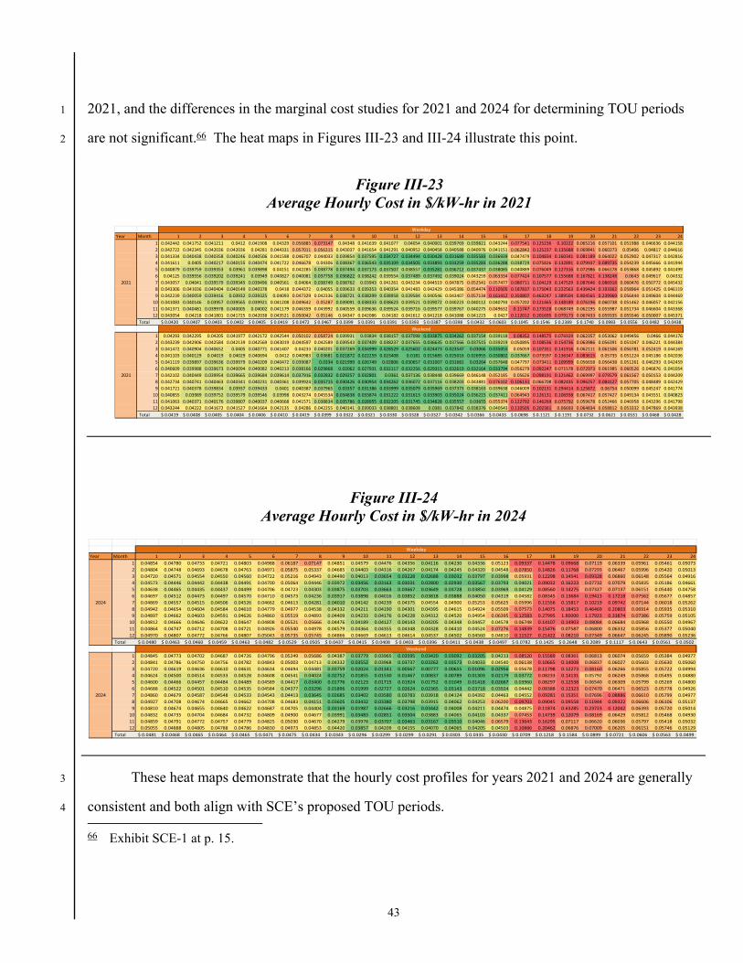
43

2021, and the differences in the marginal cost studies for 2021 and 2024 for determining TOU periods 1

are not significant.66 The heat maps in Figures III-23 and III-24 illustrate this point. 2

Figure III-23 Average Hourly Cost in $/kW-hr in 2021

Figure III-24 Average Hourly Cost in $/kW-hr in 2024

These heat maps demonstrate that the hourly cost profiles for years 2021 and 2024 are generally 3

consistent and both align with SCE’s proposed TOU periods. 4


Year Month 1 2 3 4 5 6 7 8 9 10 11 12 13 14 15 16 17 18 19 20 21 22 23 241 0.042442 0.041752 0.041211 0.0412 0.041908 0.04329 0.056885 0.073147 0.04348 0.041639 0.041077 0.04054 0.040001 0.039769 0.039821 0.043244 0.077541 0.125236 0.10222 0.065216 0.057101 0.051988 0.046636 0.0441582 0.042722 0.042345 0.042036 0.042036 0.04281 0.044331 0.057011 0.056315 0.043037 0.041654 0.041291 0.040952 0.040458 0.040588 0.040976 0.041151 0.062842 0.125237 0.135688 0.069841 0.060273 0.05406 0.04817 0.0446163 0.041334 0.040438 0.040358 0.040246 0.040506 0.041598 0.046707 0.044033 0.039854 0.037595 0.034727 0.034494 0.030428 0.031689 0.035583 0.036939 0.047479 0.104834 0.160341 0.081189 0.064022 0.052902 0.047317 0.0428164 0.041611 0.0405 0.040217 0.040155 0.040474 0.041722 0.046678 0.04306 0.038367 0.036543 0.035109 0.034505 0.033893 0.033259 0.035283 0.036288 0.038729 0.075826 0.132891 0.079937 0.089735 0.054239 0.045666 0.0419445 0.040879 0.039759 0.039353 0.03961 0.039898 0.04151 0.042285 0.038778 0.037494 0.037173 0.037507 0.038557 0.035281 0.036712 0.037437 0.038085 0.040889 0.076049 0.127316 0.072986 0.066178 0.053868 0.045892 0.0414996 0.04125 0.039556 0.039202 0.039241 0.03949 0.040827 0.040081 0.037758 0.036822 0.038242 0.039554 0.037489 0.037492 0.039024 0.043259 0.063334 0.077424 0.107577 0.155688 0.167821 0.138248 0.0643 0.049617 0.043327 0.043057 0.04041 0.039579 0.039345 0.039496 0.040561 0.04064 0.038749 0.038762 0.03943 0.041261 0.043234 0.044519 0.047875 0.052541 0.057477 0.080711 0.104129 0.147529 0.087646 0.086918 0.060476 0.050772 0.0454328 0.043306 0.041036 0.040404 0.040149 0.040378 0.0418 0.044372 0.04055 0.039633 0.039353 0.040354 0.041483 0.042429 0.045386 0.054474 0.110505 0.187837 0.175043 0.222563 0.439424 0.193362 0.058964 0.051425 0.0461199 0.042239 0.040059 0.039416 0.03932 0.039325 0.04093 0.047329 0.042336 0.038721 0.038299 0.038958 0.039584 0.040546 0.043407 0.057134 0.161412 0.350807 0.463247 1.389504 0.804565 0.239969 0.056444 0.049604 0.044469

10 0.041083 0.040146 0.03957 0.039565 0.039921 0.041208 0.049642 0.05287 0.039091 0.038333 0.038623 0.039521 0.039072 0.040223 0.040112 0.040793 0.057202 0.121465 0.148189 0.076196 0.060738 0.051462 0.046057 0.04215611 0.041371 0.040481 0.039978 0.040005 0.04002 0.041179 0.046359 0.043992 0.040559 0.039636 0.039524 0.039716 0.039577 0.039767 0.040275 0.049632 0.11747 0.173528 0.068749 0.062195 0.055987 0.051734 0.046604 0.04336812 0.043054 0.04218 0.041801 0.041725 0.042038 0.043521 0.050042 0.05146 0.04347 0.042086 0.04182 0.041612 0.041218 0.041088 0.041223 0.0427 0.112012 0.201695 0.079173 0.067433 0.059335 0.055546 0.050007 0.045371

Total 0.0420$ 0.0407$ 0.0403$ 0.0402$ 0.0405$ 0.0419$ 0.0472$ 0.0467$ 0.0399$ 0.0391$ 0.0391$ 0.0393$ 0.0387$ 0.0398$ 0.0432$ 0.0603$ 0.1045$ 0.1546$ 0.2389$ 0.1740$ 0.0983$ 0.0556$ 0.0482$ 0.0438$

1 0.04293 0.042295 0.04205 0.041977 0.042172 0.042544 0.050102 0.058724 0.039931 0.03834 0.038157 0.037098 0.033875 0.034262 0.037154 0.039118 0.08352 0.148575 0.076929 0.062357 0.053062 0.049456 0.0466 0.0441762 0.043239 0.042906 0.042584 0.042139 0.042569 0.043019 0.044597 0.042589 0.039543 0.037409 0.038237 0.037655 0.036635 0.037566 0.037515 0.039219 0.050895 0.108536 0.154736 0.063986 0.056391 0.051047 0.046221 0.0443843 0.041472 0.040904 0.040652 0.0405 0.040771 0.041407 0.04233 0.040201 0.037269 0.034999 0.028529 0.025602 0.024473 0.023547 0.03066 0.035055 0.05059 0.107351 0.141916 0.062111 0.061506 0.056781 0.052419 0.0441694 0.041103 0.040129 0.04019 0.04029 0.040694 0.0412 0.040983 0.03681 0.021872 0.022259 0.023408 0.0181 0.015685 0.025016 0.026955 0.030802 0.037667 0.073597 0.136347 0.083615 0.05735 0.051224 0.045186 0.0420365 0.041119 0.039897 0.039636 0.039979 0.040209 0.040472 0.039087 0.0334 0.021999 0.026749 0.02806 0.030657 0.031007 0.031681 0.03264 0.037648 0.047797 0.073411 0.109999 0.056658 0.056438 0.051261 0.046293 0.0424596 0.040609 0.039988 0.039673 0.040094 0.040082 0.040213 0.038166 0.029868 0.02062 0.027931 0.032117 0.032256 0.029315 0.032619 0.032164 0.033794 0.056279 0.092247 0.071578 0.072973 0.061985 0.060526 0.046876 0.0410547 0.042102 0.040449 0.039954 0.039665 0.039684 0.039614 0.037916 0.032832 0.029257 0.032801 0.0361 0.037136 0.038448 0.039669 0.046148 0.052185 0.05626 0.098191 0.121462 0.069997 0.079579 0.061567 0.050153 0.0442098 0.042734 0.040741 0.040463 0.040341 0.040231 0.040361 0.039924 0.035715 0.030426 0.030954 0.034262 0.036072 0.037116 0.038203 0.043881 0.076102 0.106131 0.066708 0.082435 0.096257 0.084127 0.057705 0.048489 0.0424299 0.041721 0.040378 0.039834 0.03937 0.039433 0.0401 0.040387 0.037965 0.03357 0.031386 0.033999 0.035079 0.035969 0.037373 0.038163 0.039638 0.046009 0.102131 0.294414 0.125872 0.06754 0.050099 0.045247 0.041774

10 0.040855 0.03989 0.039752 0.039579 0.039546 0.03998 0.043274 0.045534 0.034838 0.033874 0.031222 0.031613 0.033903 0.035024 0.036215 0.037411 0.064943 0.126131 0.106938 0.067417 0.057427 0.049134 0.043551 0.04082311 0.041063 0.040371 0.040176 0.039807 0.040037 0.040668 0.041571 0.038834 0.035786 0.028955 0.032205 0.031745 0.034828 0.035557 0.03655 0.055374 0.122792 0.146269 0.075792 0.059678 0.052466 0.046958 0.043296 0.04179812 0.043244 0.04222 0.041672 0.041527 0.041664 0.042135 0.04286 0.042255 0.040141 0.039033 0.038801 0.038608 0.0381 0.037842 0.038376 0.040543 0.110505 0.202361 0.06693 0.064834 0.058812 0.053332 0.047869 0.043938

Total 0.0419$ 0.0408$ 0.0405$ 0.0404$ 0.0406$ 0.0410$ 0.0419$ 0.0399$ 0.0322$ 0.0321$ 0.0330$ 0.0328$ 0.0327$ 0.0342$ 0.0366$ 0.0433$ 0.0698$ 0.1121$ 0.1191$ 0.0732$ 0.0621$ 0.0531$ 0.0468$ 0.0428$

Weekday

2021

2021

Weekend

Year Month 1 2 3 4 5 6 7 8 9 10 11 12 13 14 15 16 17 18 19 20 21 22 23 241 0.04854 0.04780 0.04733 0.04721 0.04803 0.04988 0.06187 0.07147 0.04851 0.04579 0.04476 0.04356 0.04116 0.04230 0.04336 0.05123 0.09337 0.14478 0.09668 0.07119 0.06339 0.05961 0.05461 0.050732 0.04804 0.04748 0.04693 0.04678 0.04763 0.04971 0.05875 0.05337 0.04685 0.04403 0.04316 0.04267 0.04174 0.04245 0.04320 0.04548 0.07850 0.14826 0.11768 0.07293 0.06467 0.05996 0.05420 0.050133 0.04720 0.04571 0.04554 0.04550 0.04560 0.04722 0.05216 0.04943 0.04490 0.04013 0.03654 0.03228 0.02688 0.03032 0.03797 0.03998 0.05931 0.12298 0.14541 0.09328 0.06860 0.06148 0.05564 0.049164 0.04573 0.04446 0.04442 0.04438 0.04491 0.04700 0.05064 0.04446 0.03972 0.03456 0.03163 0.03031 0.02800 0.02930 0.03567 0.03793 0.04021 0.09032 0.16223 0.07732 0.07079 0.05835 0.05186 0.046615 0.04638 0.04465 0.04435 0.04437 0.04499 0.04706 0.04723 0.04303 0.03875 0.03703 0.03663 0.03667 0.03649 0.03728 0.03850 0.03969 0.04129 0.08560 0.14275 0.07327 0.07137 0.06151 0.05440 0.047586 0.04697 0.04512 0.04473 0.04497 0.04570 0.04710 0.04573 0.04236 0.03917 0.03898 0.04016 0.03852 0.03818 0.03888 0.04050 0.04319 0.04582 0.08345 0.13684 0.19413 0.17218 0.07562 0.05677 0.048577 0.04869 0.04557 0.04515 0.04506 0.04526 0.04662 0.04613 0.04281 0.04010 0.04142 0.04239 0.04375 0.04554 0.04900 0.05253 0.05625 0.05996 0.11556 0.15817 0.10219 0.09742 0.07144 0.06018 0.052628 0.04942 0.04654 0.04604 0.04584 0.04610 0.04779 0.04977 0.04538 0.04332 0.04211 0.04190 0.04301 0.04395 0.04615 0.04924 0.05509 0.07573 0.14075 0.18453 0.46469 0.20803 0.06914 0.05935 0.053109 0.04897 0.04662 0.04603 0.04591 0.04626 0.04860 0.05519 0.04893 0.04409 0.04233 0.04176 0.04228 0.04312 0.04520 0.04954 0.06395 0.12583 0.27995 1.80000 1.17923 0.33874 0.07386 0.05759 0.05105

10 0.04812 0.04666 0.04646 0.04622 0.04647 0.04808 0.05521 0.05666 0.04476 0.04189 0.04127 0.04143 0.04205 0.04348 0.04457 0.04578 0.06748 0.14107 0.14903 0.08084 0.06684 0.05968 0.05550 0.0496711 0.04864 0.04747 0.04712 0.04708 0.04721 0.04926 0.05540 0.04978 0.04579 0.04364 0.04355 0.04348 0.04328 0.04410 0.04524 0.07276 0.14839 0.15476 0.07587 0.06800 0.06332 0.05856 0.05377 0.0504012 0.04970 0.04807 0.04772 0.04766 0.04807 0.05043 0.05735 0.05745 0.04866 0.04669 0.04613 0.04614 0.04537 0.04502 0.04560 0.04810 0.11527 0.21422 0.08210 0.07349 0.06647 0.06245 0.05890 0.05236

Total 0.0480$ 0.0463$ 0.0460$ 0.0459$ 0.0463$ 0.0482$ 0.0529$ 0.0505$ 0.0437$ 0.0415$ 0.0408$ 0.0403$ 0.0396$ 0.0411$ 0.0438$ 0.0497$ 0.0782$ 0.1425$ 0.2648$ 0.2089$ 0.1117$ 0.0643$ 0.0561$ 0.0502$

1 0.04845 0.04773 0.04702 0.04687 0.04726 0.04796 0.05249 0.05686 0.04387 0.03779 0.03965 0.03595 0.03420 0.03092 0.03205 0.04213 0.08520 0.15589 0.08361 0.06813 0.06074 0.05659 0.05384 0.049772 0.04841 0.04786 0.04750 0.04756 0.04782 0.04843 0.05003 0.04713 0.04332 0.03552 0.03968 0.03737 0.03262 0.03573 0.04033 0.04540 0.06138 0.10665 0.14008 0.06837 0.06027 0.05603 0.05630 0.050603 0.04720 0.04619 0.04636 0.04610 0.04631 0.04634 0.04694 0.04481 0.03759 0.02024 0.01341 0.00567 0.00777 0.00655 0.01096 0.02956 0.05678 0.11798 0.12273 0.08160 0.06266 0.05855 0.05722 0.049944 0.04624 0.04500 0.04514 0.04533 0.04528 0.04608 0.04541 0.04024 0.02752 0.01855 0.01530 0.01467 0.00837 0.00789 0.01303 0.02179 0.03772 0.08233 0.14131 0.05792 0.06249 0.05868 0.05495 0.048805 0.04600 0.04466 0.04457 0.04484 0.04489 0.04589 0.04417 0.03400 0.01776 0.02123 0.01715 0.01924 0.01752 0.01049 0.01418 0.02667 0.03960 0.08297 0.12538 0.06540 0.06309 0.05799 0.05269 0.048006 0.04688 0.04522 0.04501 0.04510 0.04535 0.04584 0.04377 0.03296 0.01896 0.01999 0.02727 0.02624 0.02365 0.03143 0.03718 0.03924 0.04442 0.08388 0.12323 0.07470 0.06471 0.06523 0.05778 0.049267 0.04860 0.04679 0.04587 0.04548 0.04533 0.04543 0.04413 0.03645 0.02685 0.03402 0.03580 0.03783 0.03918 0.04124 0.04392 0.04463 0.04552 0.09281 0.15351 0.07696 0.08886 0.06610 0.05799 0.049778 0.04927 0.04708 0.04674 0.04665 0.04662 0.04708 0.04683 0.04151 0.03605 0.03432 0.03380 0.03798 0.03915 0.04062 0.04253 0.06200 0.09703 0.09045 0.09558 0.11944 0.09322 0.06606 0.06106 0.051379 0.04810 0.04674 0.04655 0.04640 0.04622 0.04687 0.04705 0.04404 0.03169 0.01987 0.02666 0.03216 0.03442 0.04008 0.04211 0.04474 0.04875 0.11874 0.63285 0.23723 0.12042 0.06393 0.05720 0.05014

10 0.04832 0.04735 0.04704 0.04684 0.04732 0.04809 0.04900 0.04677 0.03991 0.03483 0.02851 0.03504 0.03883 0.04065 0.04103 0.04337 0.07453 0.14739 0.12079 0.08169 0.06429 0.05812 0.05468 0.0493011 0.04859 0.04791 0.04772 0.04757 0.04779 0.04825 0.05030 0.04670 0.04279 0.03978 0.03707 0.03463 0.03167 0.03510 0.04046 0.06579 0.13643 0.16295 0.07117 0.06620 0.06036 0.05797 0.05418 0.0503212 0.05055 0.04888 0.04805 0.04788 0.04786 0.04830 0.04973 0.04853 0.04420 0.03857 0.04209 0.04155 0.04070 0.04065 0.04205 0.04503 0.10886 0.20462 0.06876 0.07009 0.06205 0.06151 0.05746 0.05129

Total 0.0481$ 0.0468$ 0.0465$ 0.0464$ 0.0465$ 0.0471$ 0.0475$ 0.0434$ 0.0343$ 0.0296$ 0.0299$ 0.0299$ 0.0291$ 0.0303$ 0.0335$ 0.0430$ 0.0709$ 0.1218$ 0.1584$ 0.0899$ 0.0721$ 0.0606$ 0.0563$ 0.0499$

Weekday

2024

Weekend

2024

44

F. Elimination of the Proposed Super-Off-Peak Period 1

In testimony, SEIA states that it does not support SCE’s proposal to establish a permanent winter 2

SOP period. SEIA’s rationale is that the conditions that drive the adoption of a midday SOP period are 3

not expected to be present on every day of the winter season, and a more preferred option is to develop a 4

“Discount Days” program to address specific periods of low prices in the middle of the day.67 5

First, SEIA’s Discount Days concept is outside the scope of this proceeding, as it addresses rate 6

design and not the establishment of standard TOU periods.68 Second, with regard to the appropriateness 7

of a winter SOP period, SCE’s proposed TOU periods are based on the clustering of hours when costs, 8

on average, are expected to be fairly consistent. Exhibit SCE-1 presented extensive analysis regarding 9

the establishment of the winter SOP period, which the Commission should adopt.69 The establishment 10

of an SOP period and the accompanying retail rate design also allows customers to actively participate 11

in modifying consumption behavior in a manner that alleviates CAISO-system-level operating 12

constraints that are caused by oversupply conditions typically prevalent in SCE’s proposed SOP period, 13

as discussed in Exhibit SCE-2.70 14

G. Discussion of SEIA’s Other TOU Period Proposals 15

In addition to proposing a 2 p.m. to 8 p.m. on-peak period, SEIA also proposes (1) no 16

differentiation between day types (i.e., weekdays and weekends) and (2) a confusing bifurcated summer 17

mid-peak period. SCE addresses these additional TOU period proposals, as follows. 18

1. SEIA’s Aggregation of Weekdays and Weekends Is Inappropriate 19

In testimony, SEIA proposes no differentiation between weekdays and weekends,71 20

which is not supported by relevant cost data. Table III-9 shows SEIA’s own proposed average monthly 21


68 See SCE’s June 1, 2017 Motion to Strike Testimony submitted in this proceeding at pp. 3-4.

69 Exhibit SCE-1 at pp. 58-65, 73.



45

total costs for each day type throughout the year. This data is presented at the hourly level in Figure III-1

25, based on SEIA’s definition of summer. 2

Table III-9 Average Day Type Hourly Cost Comparison ($/MWh)

Month

Monthly Average Cost

/ Hour

Monthly Weekdays

Average Cost / Hour

Monthly Weekends

Average Cost / Hour

Weekday Average / Monthly Average

Weekend Average / Monthly Average

1 52.7 53.1 52.0 1% -2% 2 53.0 54.0 51.0 2% -6% 3 49.0 49.5 47.9 1% -3% 4 46.5 47.4 44.1 2% -7% 5 45.2 46.5 43.0 3% -7% 6 55.5 58.2 48.2 5% -17% 7 58.3 62.0 50.6 6% -18% 8 194.8 237.2 91.1 22% -62% 9 154.5 191.2 68.6 24% -64%

10 56.2 57.6 53.3 2% -8% 11 50.7 52.4 47.6 3% -9% 12 56.5 56.6 56.4 0% 0%

Annual 72.9 80.5 54.5 10% -32%

46

Figure III-25 SEIA’s Summer Weekday / Weekend Hourly Average Total Costs ($/MWh)

While the average daily cost differentials between day types is relatively small during the 1

winter months, the same does not hold true for the summer season. The large differentials, especially 2

for August and September, do not support SEIA’s proposal to keep day types in the same TOU period 3

throughout the entire year, particularly in the summer season. On the other hand, to help address these 4

cost-based differentials, SCE’s TOU period proposal appropriately distinguishes between day types 5

when setting the TOU periods by designating 4 p.m. to 9 p.m. on weekdays in the summer as “on-peak,” 6

and 4 p.m. to 9 p.m. on weekends in the summer as “mid-peak.”72 7

72 See also Figures III-6 and III-9 through III-12.

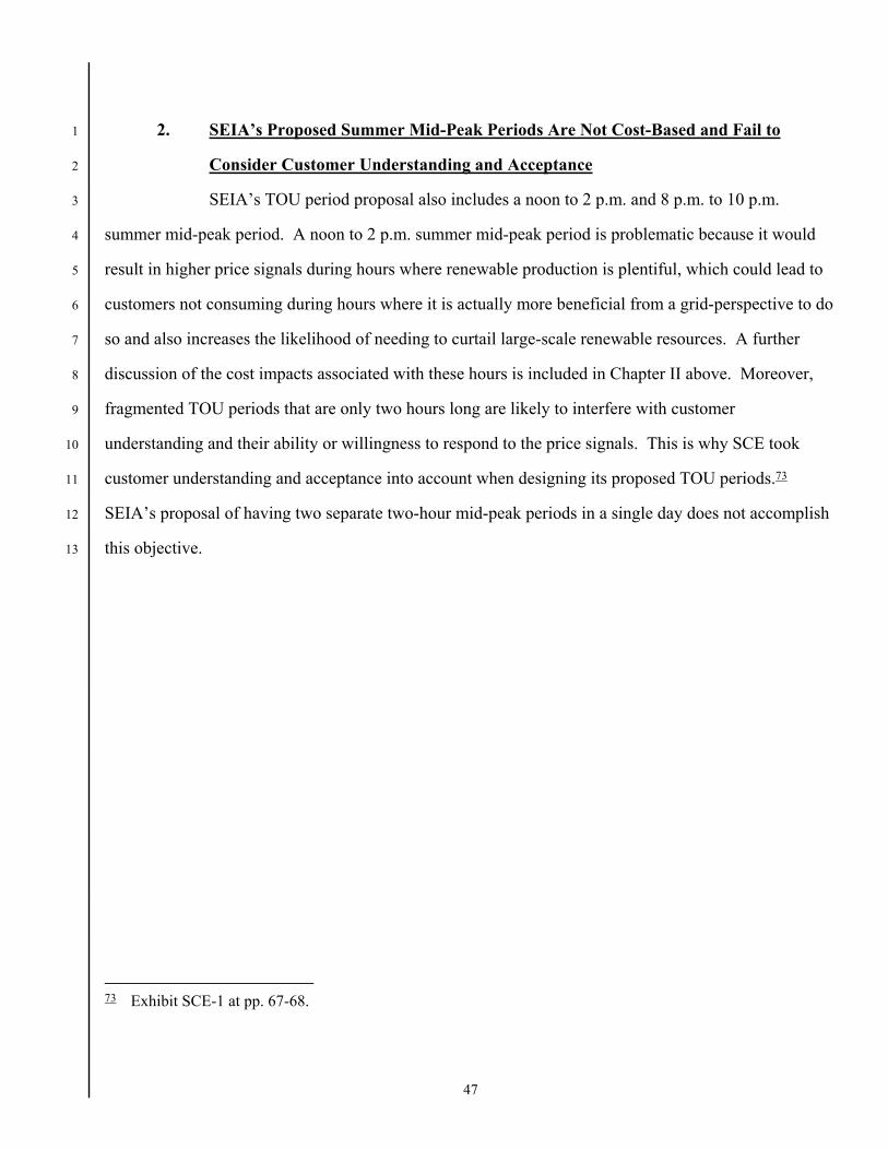
47

2. SEIA’s Proposed Summer Mid-Peak Periods Are Not Cost-Based and Fail to 1

Consider Customer Understanding and Acceptance 2

SEIA’s TOU period proposal also includes a noon to 2 p.m. and 8 p.m. to 10 p.m. 3

summer mid-peak period. A noon to 2 p.m. summer mid-peak period is problematic because it would 4

result in higher price signals during hours where renewable production is plentiful, which could lead to 5

customers not consuming during hours where it is actually more beneficial from a grid-perspective to do 6

so and also increases the likelihood of needing to curtail large-scale renewable resources. A further 7

discussion of the cost impacts associated with these hours is included in Chapter II above. Moreover, 8

fragmented TOU periods that are only two hours long are likely to interfere with customer 9

understanding and their ability or willingness to respond to the price signals. This is why SCE took 10

customer understanding and acceptance into account when designing its proposed TOU periods.73 11

SEIA’s proposal of having two separate two-hour mid-peak periods in a single day does not accomplish 12

this objective.13


48

IV. 1

REBUTTAL TO ORA’S TOU PERIOD TESTIMONY 2

ORA provides direct prepared testimony of Mr. Eric Duran that assesses SCE’s proposed TOU 3

periods, in which ORA accepts certain SCE inputs and recommends modification to others.74 Overall, 4

ORA’s testimony advocates for a 3 p.m. to 8 p.m. peak period, based on ORA’s contention that a 3 p.m. 5

to 8 p.m. peak period performs nearly as well as a 4 p.m. to 9 p.m. period but represents a more gradual 6

change from existing TOU periods and mitigates bill impacts for lower usage customers.75 In making its 7

recommendation for moving to a 3 p.m. to 8 p.m. peak period, ORA relies on a regression analysis that 8

uses 2021 data and the allocation of flexible capacity costs over all three hours of the ramping period.76 9

SCE addressed ORA’s arguments in Chapter II above, with the exception of ORA’s concern over 10

customer bill impacts. As such, the following section addresses the impact of the TOU period proposals 11

on customers’ bills. 12

A. Customer Bill Impacts 13

In testimony, ORA presents analysis on the annual, seasonal and monthly bill impacts for small 14

commercial customers77 using the illustrative rates included in Appendix B of Exhibit SCE-1, and 15

concluded that SCE’s proposed TOU periods disproportionately and adversely impact small commercial 16

customers with lower average demands (kW) compared to those with higher average demands.78 ORA 17

advocates for the implementation of balanced payment plans to help mitigate these bill impacts.79 18

74 Specifically, ORA accepted or did not object to (1) the marginal cost values SCE used to determine TOU

periods, (2) SCE’s 60/40 allocation of marginal generation capacity costs between peak capacity and flexible ramping capacity costs, and (3) SCE’s determination of peak- versus grid-related components for TOU period determination. ORA objected to SCE’s use of 2024 data (as opposed to 2021 data), and SCE’s allocation of costs during the ramping period. See ORA Testimony at p. 2.

75 ORA Testimony at pp. 10-11.

76 Id. at pp. 8-9.

77 I.e., customers with maximum demands of 20 kW or less who are served on SCE’s TOU-GS-1 rate schedules.


79 Id. at p. 16.

49

First, the implementation of a balanced payment plan option is outside the scope of this 1

proceeding as it is not related to the establishment of standard TOU periods.80 2

With regard to bill impacts, ORA’s analysis and supporting testimony noted that on an annual 3

basis, there appears to be an even distribution of both positive and negative bill impacts on SCE’s 4

proposed TOU periods. However, when looking at the summer months, negative bill impacts tend to 5

outweigh positive ones.81 As described in Exhibit SCE-1, SCE’s original implementation plan for the 6

updated TOU periods would utilize the illustrative rates included in Appendix B of Exhibit SCE-1 only 7

for the period of October 1, 2018 through the implementation of SCE’s 2018 GRC Phase 2 final 8

decision, which was anticipated to be prior to the start of summer in 2019.82 As such, the illustrative 9

rates utilized by ORA to determine the summer bill impacts will never actually be used to bill customers 10

during the summer since they will be superseded by the outcome of SCE’s 2018 GRC Phase 2 11

proceeding. ORA’s bill impact analysis should therefore only focus on the winter months (October – 12

May), where ORA found minimal impact to customers’ bills. In SCE’s 2018 GRC Phase 2 application, 13

SCE will propose updated marginal costs, revenue allocation, and new rate structures that more 14

appropriately reflect the different cost drivers discussed in both proceedings. In addition, ORA is free to 15

raise additional or alternative rate design proposals in that proceeding to mitigate customer bill impacts 16

from the new TOU periods. As such, SCE’s 2018 GRC Phase 2 proceeding is a more appropriate venue 17

for a comprehensive assessment of the impacts to customers’ bills caused by the change in TOU periods 18

and associated costs. 19

80 See SCE’s June 1, 2017 Motion to Strike Testimony submitted in this proceeding at p. 5.


82 Exhibit SCE-1 at pp. 75-78. Additionally, in Chapter X herein, SCE proposes to modify its original implementation approach and align the implementation of this proceeding with SCE’s 2018 GRC Phase 2 proceeding.

50

V. 1

REBUTTAL TO AECA’S AND CFBF’S TOU PERIOD TESTIMONY 2

Both AECA and CFBF provided direct prepared testimony arguing against the adoption of 3

SCE’s proposed TOU periods, but did not propose any specific alternatives – other than deferring the 4

implementation or retaining legacy TOU periods indefinitely. The basic rationale presented by AECA 5

and CFBF in their opposition is that SCE failed to adequately consider the impacts of its TOU period 6

proposal on the agricultural community. However, SCE demonstrates in the section below that A&P 7

customers have traditionally been one of the most responsive customer segments with regard to TOU 8

periods, even before TOU periods were mandatory, and further rebuts arguments that the updated TOU 9

periods should not be mandatory for this customer segment. Testimony addressing AECA’s and 10

CFBF’s TOU period mitigation proposals (e.g., grandfathering or lump sum payments) and the preferred 11

consolidation of this proceeding with SCE’s 2018 GRC Phase 2 proceeding are addressed in Chapters 12

VII and X, respectively. Finally, SCE notes that the proposals regarding specific rate design options 13

presented by both AECA and the CFBF are outside the scope of this proceeding, and not addressed 14

herein, since they do not relate to the implementation of standard TOU periods.83 15

A. A&P Customer Responsiveness to TOU Periods 16

As acknowledged by AECA, A&P customers’ response to TOU rates is well documented.84 This 17

is especially true among pumping customers, whose use of timing devices provide a measure of control 18

not possible from other rate groups. Contrary to the testimony of AECA and CFBF, it is exactly this 19

level of flexibility that provides the A&P community with the most opportunity for savings as a result of 20

TOU period changes. Table V-10 shows the percentage of A&P load served on TOU rates when TOU 21

rates were optional for these customers (mandatory TOU for all A&P customers was implemented in 22

2014 and 2015). 23

83 See SCE’s June 1, 2017 Motion to Strike Testimony submitted in this proceeding at pp. 2-3.

84 AECA Testimony at p. 15.

51

Table V-10 Percentage of A&P Customers’ Annual Usage Served on TOU and Non-TOU

Rates % of Annual Usage

Year TOU Accounts Non-TOU Accounts

2002 67.48 32.52

2003 71.23 28.77

2004 71.53 28.47

2005 72.90 27.10

2006 73.98 26.02

2007 73.70 26.30

2008 75.68 24.32

2009 77.68 22.32

2010 80.85 19.15

2011 81.97 18.03

2012 81.03 18.97

2013 80.54 19.46

2014 87.85 12.15

2015 99.07 0.93

2016 99.96 0.04

Over 70 percent of A&P load has been served on TOU rates since 2003, and their response to 1

these TOU periods has translated into some of the lowest average rates across any customer rate group. 2

As such, in addition to doing the grid a disservice by inhibiting the shift of historically-flexible load 3

away from peak constraint periods, the attempts to delay or prohibit A&P customers with flexible load 4

from taking advantage of the updated TOU periods and associated rate structures is ill-advised. 5

Moreover, when SCE transitioned A&P customers to mandatory TOU rates in 2014 and 2015, 6

A&P customers demonstrated a greater overall response compared to other customer segments. For 7

example, when asked if they were aware of TOU rates and the transition to mandatory TOU, 8

approximately 70 percent of A&P customers responded in the affirmative – a significantly higher 9

percentage compared to other customer segments. When asked if they understood the need to manage 10

electricity use differently on TOU rates, A&P customers had the highest affirmative response. Finally, 11

in post-implementation surveys, A&P customers also demonstrated their responsiveness to TOU periods 12

52

by taking various actions to manage electricity usage such as reducing electric consumption, adjusting 1

hours of use and changing equipment. 2

B. Updated TOU Periods Must Be Mandatory 3

CFBF argues in testimony that any new TOU periods should be implemented on an optional 4

basis only until such time, if ever, that there is more clarity as to what the correct TOU periods will be 5

for at least a 10-year period.85 This position is counter to the Commission’s findings in the recent TOU 6

OIR decision (D.17-01-006), which adopts a framework, including guiding principles, for designing, 7

implementing and modifying the time intervals reflected in TOU rates. In that decision, the 8

Commission provided its rationale for updating TOU periods: 9

“By varying retail price signals in relation to utility costs, TOU rates better reflect cost causation 10

and motivate customers to shift their usage to periods that promote more efficient use of the 11

electrical system. This shift should assist in reaching state energy goals by minimizing costs, 12

encouraging energy conservation at appropriate times, and increasing electric supply at times 13

that best serve the needs of the electrical grid.”86 14

Allowing customers to remain on outdated legacy TOU periods with price signals that encourage 15

consumption during times when the system is most constrained, as CFBF is requesting, not only hinders 16

the ability of the state to achieve its clean energy goals but also results in increased costs for all 17

customers due to the investments utilities would have to make to mitigate system constraints – which 18

defeats the purpose of implementing TOU pricing in the first place. 19

CFBF’s further recommendation that updated TOU periods only become mandatory when there 20

is more clarity around what the TOU periods should be 10 years out is also counter to the direction 21

provided in D.17-01-006. In that decision, the Commission requires utilities to develop base TOU 22

periods using forward-looking data, with the forecast year set at least three years after the new TOU 23

periods take effect. The decision also requires that these base TOU periods continue for a minimum of 24

85 CFBF Testimony at p. 15.

86 D.17-01-006 at pp. 3-4.

53

five years, unless material changes in relevant assumptions indicate the need for more frequent base 1

TOU period revisions.87 SCE’s use of forecasted 2024 data to develop its proposed TOU period 2

updates, which CFBF somewhat ironically rejects as being “too-forward looking,” satisfies these 3

requirements and should result in stable TOU periods for the timeframe envisioned by the decision.88 4

Finally, CFBF argues that SCE should not implement “mandatory rate designs without 5

developing alternative rate design options tailored to particular customer classes or customer types,” and 6

cites three policy guidelines in D.17-01-006 to support its position.89 As noted in its Motion to Strike, 7

the scope of this proceeding is to revise and implement updates to the standard TOU periods.90 Changes 8

to rate design associated with the updated TOU periods is not in scope for this proceeding, and neither is 9

the “menu of TOU options” referenced in D.17-01-006. As such, these arguments should bear no 10

weight with regard to the adoption of the proposed mandatory changes to standard TOU periods, which 11

is the specific item in scope for this proceeding. 12

87 Id. at p. 7.



90 See SCE’s June 1, 2017 Motion to Strike Testimony submitted in this proceeding at p. 3.

54

VI. 1

REBUTTAL TO SBUA’S TOU PERIOD TESTIMONY 2

SBUA provides direct prepared testimony of Amy Macaux and Daniela Laakso. In that 3

testimony, SBUA indicates that SCE’s proposed TOU periods “may be fair,”91 provided SCE eliminates 4

the separate summer weekday and weekend periods and instead applies a single “peak” rate during 4 5

p.m. to 9 p.m.92 SBUA further argues that SCE must substantially improve its marketing, education and 6

outreach (ME&O) strategy to ensure small business customers understand the new TOU periods and are 7

able to respond to them by (1) hiring an outside marketing firm to design an effective ME&O campaign, 8

(2) providing “shadow” bills to small business customers to show them how their electricity costs will 9

be impacted if they don’t take any action, and (3) tying the success of SCE’s ME&O campaign to actual 10

shifts in usage by small business customers.93 Finally, SBUA puts forth other DG and storage proposals 11

to help promote California’s clean energy goals94 – all of which are outside the scope of this 12

proceeding.95 SCE addresses the recommendations made by SBUA in the section below. 13

A. Combination of the Summer On- and Mid-Peak Periods 14

In testimony, SBUA recommends that SCE combine the summer weekday on-peak period and 15

weekend mid-peak period into a single summer peak rate.96 Both periods occur from 4 p.m. to 9 p.m. in 16

the summer season, but the on-peak period is only for weekdays and the mid-peak period applies to 17

weekends. SBUA argues that combining the periods into a single rate aligns with the preference of 18

small business customers who prefer spreading the highest peak rate over all seven days, which can 19

91 SBUA Testimony at p. 15.

92 Id. at p. 13.

93 Id. at pp. 18-24.

94 Id. at pp. 27-35.

95 SCE did not receive SBUA’s testimony until June 2, 2017, and was therefore unable to include these items in the Motion to Strike Testimony filed June 1, 2017. SCE intends to file a motion to strike the items in SBUA’s testimony that are not within the scope of this proceeding.

96 Id. at p. 13.

55

reduce the peak weekday rates.97 SBUA also states that a reduced number of periods is easier for 1

customers to understand and respond to.98 2

For the reasons discussed in Chapter III.G.1, SCE does not agree with SBUA’s recommendation. 3

Again, while the average daily cost differentials between day types is relatively small during the winter 4

months, the same does not hold true for the summer season. Accordingly, the relatively large cost 5

differentials between weekdays and weekends, especially for August and September, support SCE’s 6

proposal to distinguish between day types when setting the summer TOU periods. Moreover, SBUA’s 7

proposal would have the effect of increasing rates during the weekend, which conflicts with the requests 8

of other parties, such as CFBF, who advocate for lower weekend rates.99 The determination of TOU 9

periods needs to balance the impacts to all customers, along with the associated underlying costs. 10

B. ME&O Efforts for Small Business Customers 11

SBUA argues that SCE must “substantially improve” its ME&O efforts to ensure small business 12

customers understand and can respond to the changing TOU periods, and offers three recommendations 13

for SCE to incorporate into its proposed ME&O plan. In Exhibit SCE-1, SCE provides testimony on its 14

ME&O plan,100 and recommends that the Commission adopt that plan as opposed to the 15

recommendations made by SBUA for the reasons discussed below. 16

1. SCE Already Utilizes Outside Agencies for Its ME&O Campaigns 17

In testimony, SBUA recommends that SCE hire a third-party marketing and advertising 18

firm to design effective TOU messaging for small business customers. SCE does utilize outside 19

marketing firms and advertising agencies for its ME&O campaigns, and intends to do so again when 20

developing the new TOU period ME&O materials, including those created for small businesses. The 21

ME&O sample cited in Exhibit 10 of SBUA’s testimony was developed by an outside agency and 22

97 Id. at p. 14.

98 Id.


100 SBUA Testimony at pp. 81-81.

56

represented just one ME&O channel (i.e., direct mail newsletter) that was used to communicate TOU 1

period awareness in 2013 and 2014. 2

SCE has already engaged an outside marketing firm to assist SCE in communicating the 3

proposed TOU period and CPP changes. This outside firm has begun to conduct market research with 4

impacted customer groups, including small businesses, to better understand how to effectively 5

communicate the updates proposed by SCE. SCE believes these activities largely address this first 6

recommendation made by SBUA. 7

2. “Shadow” Bills Have Limited Benefits Compared to the Costs 8

In testimony, SBUA recommends that SCE provide “shadow” or “mock” bills to small 9

business customers beginning six months prior to the date that the new TOU periods are implemented.101 10

These mock bills would show customers what their bills would have looked like if the new TOU periods 11

were in effect, and would also include information on how to respond to the updated TOU periods to 12

mitigate bill impacts. 13

SCE sees little value in providing shadow bills compared to the costs associated with 14

doing so. In order to provide shadow billing, costly billing system modifications and expedited 15

implementation timeframes would be required to create “mock” bills that may or may not be used by 16

customers. Instead, SCE plans to provide traditional rate comparisons that accomplish a similar 17

objective as shadow bills in a more cost-effective manner by utilizing either SCE’s existing rate analysis 18

methods and/or providing specific bill impact communications to the most impacted customers 19

(including small businesses). These rate analyses utilize historical usage data and estimated rate 20

forecasts to help customers ascertain the impacts of the TOU period and/or CPP changes. These more 21

cost-effective methods align with the findings in the “Hiner Report” cited in SBUA’s testimony, which 22

indicated that it was “important to present customers with concrete rate comparisons based on their 23

101 Id. at p. 22.

57

actual usage, so that they can make apples-to-apples comparisons.”102 The findings did not indicate a 1

customer preference specifically for shadow bills. 2

3. Mandating Ongoing ME&O Efforts Based on Actual Small Business Customer 3

Usage Changes is Not Reasonable 4

In testimony, SBUA recommends that SCE continue its ME&O efforts until at least 50 5

percent of small business customers actually shift at least 10 percent of their load outside of the new on-6

peak period.103 While SCE’s planned ME&O efforts will evaluate whether small business customers 7

understand the TOU period messaging and/or modify their usage, it is not reasonable to mandate 8

ongoing ME&O efforts indefinitely based on customer behavior that SCE cannot ultimately control. 9

Rather, SCE proposes to evaluate the effectiveness of its ME&O campaign based on customers’ 10

understanding of the TOU period changes and the effort being made by customers to respond. 11

For example, after the implementation of mandatory TOU for small business customers, 12

SCE conducted a “2015 Summer Campaign Effectiveness Study” to assess the effectiveness of the 2015 13

summer marketing campaign. Surveys were conducted with approximately 300 small business 14

customers to determine (1) their awareness of TOU rates (particularly the summer on-peak rate) and (2) 15

action taken in response to the campaign’s messaging. The study concluded that a majority of the small 16

businesses surveyed were making some effort to try to reduce their on-peak usage.104 17

Based on the responses received to these types of surveys, SCE would then be in a better 18

position to determine if any follow-up messaging is necessary. SCE should not be mandated to spend an 19

unlimited amount of money on ME&O campaigns based on some arbitrary and uncontrollable target, as 20

102 Id. at p. 21.

103 Id. at p. 23.

104 When asked “how much effort is your business making this summer to save electricity during peak hours from noon to 6 p.m.,” 66 percent responded that they were making some effort to reduce usage during the peak period. Approximately 19 percent reported they were not making much effort, and 14 percent indicated they were making no effort at all.

58

SBUA recommends. Rather, SCE should assess the effectiveness of its campaign and have the 1

flexibility to determine any follow-up actions that are needed based on the results. 2

C. SBUA’s Other Clean Energy Proposals 3

SBUA’s testimony concludes with a section dedicated to additional steps that SCE should take to 4

address the impacts of the new TOU periods on California’s efforts to promote clean energy. These 5

include (1) launching a free “SCE Small Business Energy Storage Pilot” for small business customers 6

who have invested in DG and are not eligible for grandfathering; (2) providing “TOU Change Rebates” 7

to offset the costs of items identified in the new Small Business Energy Storage Pilot; (3) expanding the 8

eligibility of small business customers to participate in the Self-Generation Incentive Program (SGIP); 9

and, (4) requiring SCE to study whether additional rate structures might also ensure continued DG and 10

storage investment.105 None of these proposals are in scope for this proceeding, as they do not 11

specifically relate to the determination of standard TOU periods for non-residential customers. SBUA 12

acknowledges this, in part, by stating that “[w]e appreciate that the development of such an alternative 13

rate may well be beyond the scope of this RDW proceeding.” 14

105 SBUA Testimony at pp. 29-35.

59

VII. 1

REBUTTAL TO PARTIES’ TOU PERIOD MITIGATION REQUESTS 2

Multiple parties request that various mitigation measures be adopted to reduce the perceived 3

negative impacts of migrating customers from legacy TOU periods to updated TOU periods.106 These 4

mitigation measures include extended grandfathering on legacy TOU periods107 and/or lump sum or 5

fixed indifference payments based on the bill impacts resulting from the change in TOU periods if the 6

customers agree to move to the newly-adopted TOU periods. Parties cite to Guiding Principle #7 in 7

D.17-01-006, which states that “[e]ach IOU should take steps to minimize the impact of TOU peak 8

period changes on customers who have invested in on-site renewable generation or technology to 9

conserve energy during peak periods. Regularly scheduled updates to TOU periods will provide 10

predictability for these customers. Additional steps to increase certainty around TOU periods could 11

include vintaging, legacy TOU periods, or fixed indifference payments, as well as other rate structures 12

that provide predetermined limits on TOU period changes. Such steps must also include making 13

information on potential shifts in peak periods available to the public.”108 While SCE maintains that the 14

consideration of these mitigation measures is not within the scope of this proceeding,109 SCE provides 15

the following rebuttal to the arguments made by parties in favor of such mitigation measures. 16

A. Extended Grandfathering on Legacy TOU Periods Should Be Rejected 17

AECA, CLWA, RCWD and REWD all submitted testimony requesting that the Commission 18

adopt extended grandfathering on legacy TOU periods for certain customers. AECA argues that the 19

CPUC should allow A&P customers who have shifted their loads away from existing peak periods to 20

remain on rate schedules that reflect the same periods and cost differentials for up to 10 years, thereby 21

106 SEIA Testimony at p. 35; SBUA Testimony at pp. 31-32; AECA Testimony at p. 14; CLWA Testimony at p.

4; RCWD Testimony at p. 4; and, REWD Testimony at pp. 7-8.

107 Grandfathering is defined as allowing customers to retain aspects of an existing tariff even after the tariff is no longer available to other customers. See D.17-01-006 at p. 51.

108 D.17-01-006 at p. 8.

109 See generally SCE’s June 1, 2017 Motion to Strike Testimony submitted in this proceeding.

60

enabling them to recoup their investments.110 The water district parties all argue for 20 years of 1

grandfathering on legacy TOU periods for existing RES-BCT projects and/or 10 years of grandfathering 2

for new projects to mitigate the economic impacts of changing TOU periods on customers who 3

participate in the RES-BCT program, most of whom entered into long-term power purchase agreements 4

(PPAs) with third-party solar providers.111 5

As a threshold matter, the Commission has already addressed grandfathering for eligible solar 6

customers, including those participating on RES-BCT. In D.17-01-006, the Commission adopted 10-7

year grandfathering on legacy TOU periods for these customers.112 As such, parties seeking changes to 8

those grandfathering rules cannot collaterally attack that Commission decision, but rather should file a 9

Petition for Modification (PFM) of D.17-01-006. 10

Moreover, in adopting the grandfathering provision for solar customers in D.17-01-006, the 11

Commission noted as follows: 12

“Importantly, the Commission recognizes that use of grandfathering as a mechanism for 13

mitigating negative impacts from TOU period changes has two significant weaknesses: (i) it 14

results in ‘inaccurate price signals that incent customer to use more power during high-cost 15

period’ and (ii) it is not transparent to customers. Although today’s decision adopts 16

grandfathering for a specific situation, we expect that going forward the IOUs, customers, and 17

DER technology providers will develop mitigation measures that are more transparent and more 18

narrowly tailored than grandfathering.”113 19

The decision also notes that “unlike other technologies, once solar systems are configured and 20

installed it is difficult to make changes,” and “it is possible to adjust business operation schedules.”114 21

110 AECA Testimony at p. 14.

111 CLWA Testimony at p. 4; RCWD Testimony at p. 4; and, REWD Testimony at pp. 7-8.

112 D.17-01-006 at OP 5.

113 Id. at p. 48.

114 Id. at p. 49.

61

For these reasons, SCE advocates against extending grandfathering for A&P customers, both because of 1

the general negative consequences of grandfathering highlighted by the Commission and because of the 2

specific historical propensity of A&P customers in responding to TOU periods as compared to other 3

customer groups, as discussed in Chapter V.A.1. 4

B. Indifference Payments to Mitigate the Risks Associated with Third-Party PPAs Should be 5

Rejected 6

As adopted in the Scoping Memo, the intent of SCE’s TOU period proposal is to revise standard 7

TOU periods and seasons, and implement the revised standard TOU periods for all non-residential 8

customers on rate schedules with standard TOU periods.115 The determination of lump sum indifference 9

payments to mitigate the perceived impacts of updated TOU periods has nothing to do with the 10

determination of revised standard TOU periods, and is therefore out of scope for this proceeding.116 11

Moreover, all parties in this proceeding advocating for lump sum indifference payments already 12

received grandfathering protection pursuant to OP 5 of D.17-01-006. 13

115 Scoping Memo at p. 8.

116 See generally SCE’s June 1, 2017 Motion to Strike Testimony submitted in this proceeding.

62

VIII. 1

RESPONSE TO CLECA/CMTA’S TOU PERIOD AND DEMAND RESPONSE PROGRAM 2

ALIGNMENT CONCERN 3

In testimony, CLECA/CMTA express concern that the proposed implementation of SCE’s 4

proposed TOU periods creates a serious disconnect between TOU-based rates and TOU-based demand 5

response (DR) incentives, which SCE filed in A.17-01-018.117 CLECA/CMTA’s concern is that if DR 6

incentive TOU periods (specifically related to the base interruptible program (BIP)) do not align with 7

the TOU periods in the customer’s rate schedule, the customer will have an incentive to have load online 8

during the summer noon to 6 p.m. period, while the greatest need for the resource is summer (or winter) 9

from 4 p.m. to 9 p.m.118 CLECA/CMTA argue that changes to the TOU periods for retail rates and for 10

the BIP incentives must be coordinated between A.17-01-018 and this proceeding, so a discrepancy in 11

TOU periods does not occur.119 12

SCE agrees with CLECA/CMTA’s recommendation to align DR credits with the TOU periods 13

applicable to base rates. In A.17-01-018, SCE proposed to align these items in the DR Funding 14

Application mid-cycle review. However, SCE now believes that an earlier alignment and a greater level 15

of coordination between proceedings is necessary. SCE further notes that the generation and 16

distribution cost structures used as the basis for SCE’s proposed TOU periods, as well as the DR 17

incentives filed in A.17-01-018, also form the basis for the new rate structures that will be proposed in 18

SCE’s upcoming 2018 GRC Phase 2 application. While alignment on the basic structures across 19

proceedings currently exists, changes to these basic structures can occur as part of a Phase 2 proceeding 20

to address concerns related to rate simplicity, customer acceptance, bill impacts, policy goals, etc. 21

As such, SCE concurs that the DR incentive structures will need to be coordinated with the TOU 22

periods emerging from this proceeding and the rate structures resulting from SCE’s 2018 GRC Phase 2 23

117 CLECA/CMTA Testimony at A49.

118 Id.

119 Id.

63

proceeding. To facilitate this, SCE proposes that the overall incentive levels, on a $-per-kW basis, be 1

established in A.17-01-018, and the incentive structures be established in this proceeding or in SCE’s 2

2018 GRC Phase 2 proceeding depending on the timing and magnitude of the structural change. 3

64

IX. 1

REBUTTAL TO CALSEIA’S AND SEIA’S OPTION R CAP TESTIMONY 2

In testimony, both CALSEIA and SEIA argue that the existing cap on Option R participation 3

should be either temporarily or permanently removed.120 Specifically, CALSEIA recommends that the 4

Commission order SCE to make Option R available until SCE implements the final decision in its 2018 5

GRC Phase 2 proceeding, regardless of whether the existing cap is exceeded beforehand.121 SEIA 6

strongly supports removing the Option R cap in its entirety.122 In contrast, CLECA/CMTA and EUF 7

object to the temporary or permanent removal of the Option R cap as an outcome of this proceeding, 8

arguing instead that the issue should be addressed in SCE’s upcoming 2018 GRC Phase 2 proceeding123 9

– consistent with the settlement agreement adopted by the Commission in D.14-12-048.124 10

CALSEIA’s and SEIA’s two main arguments for modifying the Option R cap prior to the date 11

adopted in D.14-12-048 are (1) previous analysis has demonstrated that Option R is a cost-based and 12

revenue neutral rate; and (2) the existing Option R 400 MW cap will be reached prior to the 13

implementation of SCE’s 2018 GRC Phase 2, which creates too much regulatory uncertainty for 14

customers considering whether to install solar. In the section below, SCE addresses these arguments 15

and recommends that all issues related to Option R be addressed in SCE’s upcoming 2018 GRC Phase 2 16

proceeding. 17

120 Option R is an alternate rate option for eligible commercial and industrial customers with demands above 20

kW who install on-site renewable generation technology. Pursuant to a settlement agreement adopted by the Commission in D.14-12-048 to resolve SCE’s 2013 RDW, participation on the rate is currently capped at 400 MW of installed capacity.

121 CALSEIA Testimony at p. 3.


123 CLECA/CMTA Testimony at A52; EUF Testimony at p. 12.

124 D.14-12-048 at OP 1, and the Joint Motion of Southern California Edison Company (U 338-E), the Office of Ratepayer Advocates, the Solar Energy Industries Association, and the Natural Resources Defense Council for Approval Of Settlement Agreement at p. 14.

65

A. Previous Option R Studies Did Indicate Cost-Shifting 1

Both CALSEIA and SEIA base their proposals to suspend or eliminate the Option R cap on their 2

assertion that previous Option R analyses performed as part of the last several GRC Phase 2 proceedings 3

have shown the rate to be cost-based and revenue neutral.125 This assertion is not comprehensive. In 4

SCE’s 2013 RDW proceeding (A.13-12-015), SCE provided a study that demonstrated a cost shift 5

associated with Option R.126 This relevant detail was omitted in CALSEIA’s and SEIA’s accounting of 6

the record in their testimony. Moreover, both entities also imply that SCE performed an Option R cost 7

study as part of its 2015 GRC Phase 2 proceeding, which, again, is erroneous. Rather, SCE’s opening 8

testimony noted that “[b]ecause SCE’s Rate R proposal is being litigated in an open proceeding [A.13-9

12-015], this 2015 GRC Phase 2 Application does not address Rate R, except to the extent that the 10

marginal costs adopted in connection with this Application will be used to update Rate R rates…”.127 11

The “update” mentioned was related to revenue allocation and rate setting, not an update of the Option R 12

cost-shift determination. 13

The cost shift study performed by SCE in its 2013 RDW proceeding was provided to support 14

SCE’s proposal to maintain the Option R participation cap. SCE’s study relied on the Energy and 15

Environmental Economics, Inc. (E3) study,128 which was required by Assembly Bill 2514 (Bradford, 16

2012) and D.12-05-036, which examined the costs and benefits of serving customers who install solar. 17

E3’s study concluded that the non-residential cost shift amounted to $70 million as of 2012 and could be 18

expected to grow to $299 million by the time the net energy metering (NEM) participation cap was 19

reached. E3’s base case scenario factored in the avoided cost of generation energy and capacity, 20

125 CALSEIA Testimony at pp. 9-15; SEIA Testimony at pp. 38-39.

126 A.13-12-015, Exhibit SCE-1 at pp. 10-12.

127 A.14-06-014, Exhibit SCE-04 at p. 21.

128 See “California Net Energy Metering Ratepayer Impacts Evaluation” (hereinafter “E3 study”), available at http://www.cpuc.ca.gov/NR/rdonlyres/D74C5457-B6D9-40F4-8584-60D4AB756211/0/NEMReportwithAppendices.pdf.

66

avoided transmission and distribution, ancillary services, avoided RPS, and avoided CO2 emissions. E3 1

described its methodology, as follows 2

“To the extent that the bill reductions attributed to NEM exceed offsetting benefits, there 3

is a cost shifting from NEM customers to other utility ratepayers. Therefore, the net cost 4

of NEM to ratepayers is the sum of ratepayer costs (bill savings, incremental billing 5

costs, and integration costs) less ratepayer benefits (avoided costs).”129 6

SCE’s cost-shift study was performed using the same basic methodology described above; 7

however, in its study, SCE only included the avoided cost of generation energy and capacity. SCE’s 8

study compared the cost shift associated with NEM customers served on the base rate, Option B, to the 9

cost shift for the same customers when served on Option R, and concluded that “[w]hen an NEM 10

customer moves from Option B to Option R, this results in a cost shift to non-participants of $142 per 1 11

kW, a cost-shift that is 200% greater than the cost-shift associated with an NEM customer on Option 12

B.”130 Based on this result, SCE proposed to maintain the Option R cap at 150 MW. SCE reiterated this 13

proposal in its 2015 GRC Phase 2 testimony,131 contrary to what CALSEIA and SEIA represent in 14

testimony. 15

B. Updated Option R Cost-Shift Analysis Has Not Been Performed 16

CALSEIA admits in testimony that it did not perform an updated cost-shift analysis of Option 17

R.132 Rather, CALSEIA attempts to argue that since new NEM customers will be served on the NEM 18

Successor Tariff adopted by the Commission in D.16-01-044, these customers will likely pay more in 19

nonbypassable charges (NBCs) and interconnection fees as a result – minimizing the cost avoided by 20

these customers. However, CALSEIA further admits that there is “some uncertainty about the cost-21

129 See “California Net Energy Metering Ratepayer Impacts Evaluation” available at

http://www.cpuc.ca.gov/NR/rdonlyres/D74C5457-B6D9-40F4-8584-60D4AB756211/0/NEMReportwithAppendices.pdf at p. 38.

130 A.13-12-015, Exhibit SCE-1 at p. 11.

131 A.14-06-014, Exhibit SCE-04 at p. 21.

132 CALSEIA Testimony at p. 14.

67

effectiveness of Option R given the changes in the NEM program and in avoided costs.”133 While D.16-1

01-044 does allow SCE to charge a $75 interconnection fee to Successor Tariff customers and does 2

require that NBCs no longer be netted, Resolution E-4792 muted the impact of the NBC change, to a 3

large extent, by requiring that the utilities continue to net NBCs in each metered interval. The result is a 4

very minimal (if any) change in the level of cost-shift associated with NBCs and customers taking 5

service on Option R. 6

C. The Option R Cap is Unlikely to be Reached Prior to the Implementation of SCE’s 2018 7

GRC Phase 2 8

In testimony, CALSEIA notes that as of April 2017, there was 124.7 MW remaining under the 9

400 MW Option R cap, and states that the Option R cap could be reached by April 2018 or sooner.134 10

SCE disagrees with CALSEIA’s conclusion. In reviewing actual participation levels since 2015, SCE 11

determined that, on average, approximately 13 MW of new installed capacity takes service on Option R 12

each quarter, as shown in Figure IX-26. 13

133 Id. at p. 15.

134 Id. SCE assumes that CALSEIA meant 2017, not 2016.

68

Figure IX-26 Option R Subscriptions (MW) by Quarter135

Assuming this trend continues, it would take roughly 27 months to reach the current Option R 1

cap. As discussed in Chapter X, SCE is proposing to implement its 2018 GRC Phase 2 in February 2

2019, which is less than 27 months from now. This analysis indicates that there is no need to upend the 3

terms of the settlement agreement adopted in D.14-12-048 by prematurely suspending or eliminating the 4

agreed-upon Option R cap, particularly when the impacts to non-participating customers have not been 5

thoroughly vetted. 6

D. Any Potential Modifications to the Option R Cap Should Be Litigated in SCE’s 2018 GRC 7

Phase 2 Proceeding 8

In accordance with the settlement agreement adopted in D.14-12-048 and for the reasons 9

discussed above, SCE agrees with the testimony of CLECA/CMTA and EUF that any potential 10

135 Data for Q2 2017 is as of May 25, 2017. The decline in Q3 2016 was the result of a large batch of projects

not submitting the necessary rate change requests in the allotted window. These customers were ultimately placed on Option R in future quarters and their participation is reflected in the overall subscription levels.

69

modifications to the Option R cap are appropriately addressed in SCE’s upcoming 2018 GRC Phase 2 1

proceeding. Both SEIA and CALSEIA were parties to the proceeding that adopted the settlement 2

agreement (and SEIA was a party to the actual settlement agreement itself), and neither party objected to 3

or opposed waiting until SCE’s next GRC to address the Option R cap. It is inappropriate to suspend or 4

outright eliminate a portion of a settlement agreement, especially when the record on the impacts to non-5

participating customers has not been developed. 6

Moreover, SCE’s 2018 GRC Phase 2 application will propose rate structures that incorporate the 7

changes proposed in this proceeding related to flexible capacity and time-differentiated distribution 8

costs. Because of the dependency on marginal costs and rate structures, the analysis of optional rates 9

and their impacts on non-participating customers are more appropriately considered as part of a GRC 10

Phase 2 proceeding. Without the knowledge of these marginal cost values and the resulting rate 11

structures, a clear determination of any Option R cost shift, and, by extension, the necessity of a 12

participation cap, cannot appropriately be made in this proceeding. 13

70

X. 1

RESPONSE TO PARTIES’ TESTIMONY REQUESTING THE CONSOLIDATION OF SCE’s 2

2016 RDW AND 2018 GRC PHASE 2 PROCEEDINGS 3

In its Application, SCE proposed to implement the revised standard TOU periods on October 1, 4

2018. Because the planned implementation would occur prior to the implementation of SCE’s 2018 5

GRC Phase 2 proceeding in which updated marginal costs, revenue allocations and rate design proposals 6

are adopted, SCE proposed the following phased-in approach with regard to rates:136 7

• Phase 1 (October 1, 2018) – rates would reflect the revised standard TOU periods using 8

the underlying marginal cost values and revenue allocations from SCE’s 2015 GRC 9

Phase 2 Marginal Cost and Revenue Allocation Settlement Agreement, adopted by D.16-10

03-030, with the exception that the 2015 GRC Phase 2 marginal energy costs (MECs) 11

would be replaced with forecast MECs that reflect the expected hourly price profiles 12

resulting from greater levels of RPS resources.137 This phase would maintain class-level 13

allocation of revenue, as well as seasonal and functional recovery of revenues. 14

• Phase 2 (Concurrent with the implementation of SCE’s 2018 GRC Phase 2) – rates would 15

reflect the revised TOU periods and the updated underlying cost drivers. 16

In testimony, SEIA, SBUA, AECA and the CFBF argue against SCE’s phased implementation 17

approach, and recommend instead that the consideration of new TOU periods should be included as part 18

of SCE’s 2018 GRC Phase 2 proceeding or at least implemented concurrently with SCE’s 2018 GRC 19

Phase 2 decision.138 ORA’s testimony indicated that it considered recommending timing the 20

implementation of the TOU periods to coincide with the implementation of 2018 GRC Phase 2 rates in 21

order to consolidate bill impacts, but was concerned that such a recommendation could further delay the 22

136 SCE’s rationale for this phased-in implementation approach is discussed in Exhibit SCE-1 at p. 79.

137 Exhibit SCE-1 at p. 75. This section additionally notes that the proposed forecast MECs would only be used in the ratesetting process to set energy charge differentials between TOU periods and ensure better alignment between costs and pricing, and would not have an effect on revenue allocation between rate groups.

138 AECA Testimony at p. 3; CFBF Testimony at p. 15; SBUA Testimony at p. 9; and, SEIA Testimony at p. 37.

71

new TOU periods given SCE’s planned billing system freeze.139 CLECA/CMTA generally supported 1

SCE’s proposed implementation approach, and specifically indicated a preference for a winter month 2

implementation (though October was not imperative) as opposed to summer, but did not support 3

delaying implementation an entire year.140 EUF supported SCE’s phased-in approach.141 4

A. SCE’s Updated Proposed Implementation Approach 5

SCE proposes to modify its recommended phased implementation approach as originally filed in 6

Exhibit SCE-1 in favor of consolidating the implementations of the TOU periods filed in this proceeding 7

with the implementation of its upcoming 2018 GRC Phase 2 proceeding.142 For the reasons described in 8

Section B below, SCE is proposing a February 2019 implementation date for both proceedings. 9

SCE agrees with parties that combining the implementations of the TOU periods with the 10

updated rates proposed in the 2018 GRC Phase 2 proceeding minimizes customer confusion, especially 11

considering the small window of time between the original October 2018 implementation date and 12

SCE’s proposed 2018 GRC Phase 2 implementation date of February 2019. A February 2019 13

implementation still provides customers approximately four months on the new TOU periods and rates 14

before the summer season, which is also preferable. 15

SCE does not propose any changes to its ME&O strategy other than to consolidate the efforts 16

previously bifurcated between Phase 1 and Phase 2.143 17

B. Customer Service Re-Platform (CSRP) Impacts 18

As discussed extensively in Exhibit SCE-01 of A.17-04-015 (SCE’s residential default TOU 19

application),144 as part of its 2018 GRC Phase 1 application (A.16-09-001), SCE proposed to replace its 20 139 ORA Testimony at p. 17.

140 CLECA/CMTA Testimony at A28.

141 EUF Testimony at p. 6.

142 While SCE supports consolidating the implementation of both proceedings, the actual issues in-scope for each proceeding (e.g., the determination of the TOU periods in this proceeding) should be litigated separately in their respective proceeding.


144 A.17-04-015, Exhibit SCE-01 at pp. 12-15.

72

obsolete Customer Service System (CSS) with a more modern, stable and agile customer technology 1

platform, i.e., the CSRP.145 The implementation of the CSRP project will limit SCE’s ability to make 2

changes to its customer service and billing systems from Q2 2019 through Q3 2020. Given this system 3

restriction, SCE is advocating for a timely resolution of the issues raised herein (and in the 2018 GRC 4

Phase 2 proceeding) to allow for implementation in the February 2019 timeframe (i.e., prior to Q2 5

2019). 6

145 The benefits of the proposed CSRP are summarized in A.17-05-015 at p. 13.

SCE-03 Rebuttal Testimony · SCE-03: Rebuttal Testimony of Southern California Edison Company Table...

Documents

Transcript of SCE-03 Rebuttal Testimony · SCE-03: Rebuttal Testimony of Southern California Edison Company Table...