Scarcity risk Premium - Lancaster University

Scarcity risk premium*

Thibault Lair†

This version: December, 2019

Abstract

This paper revisits the cost-of-carry model and proposes a decompo-sition of the futures basis that disentangles the seasonality risk premium from the scarcity risk premium. The contribution of this paper to the asset pricing literature is threefold. First, it brings novel insights on the fundamental relationship between the futures basis and inventory dynam-ics. Empirical evidence shows that the seasonality risk premium captures expectations about the inventory seasonalities while the scarcity risk pre-mium refects the excess supply and demand imbalances over the expected seasonal fuctuations. Second, this papers investigates the pricing of ex-pectations within the futures basis. Results suggest that the seasonality risk premium is priced-in and that the scarcity risk premium carries all the predictive power embedded in the futures basis. The third contribution of this paper is to provide evidence that the scarcity risk premium, and ultimately the futures basis, is mostly a compensation for the unexpected increase in the risk of stock-out and that the associated return predictabil-ity fnds its origin in the slow di˙usion of information and underreaction to abnormal changes in inventories, above and beyond seasonal dynamics.

Keywords: Commodities, theory of storage, seasonality, scarcity, risk premium, underreaction, market anomalies, factors.

*I would like to thank Frank Fabozzi, Abraham Lioui, Guido Baltussen, Alexandre de Roode, and seminar participants at the 2019 EFMA Conference and 2019 EDHEC PhD in Finance Forum for valuable discussions and useful feedback. Comments are welcomed, including references to related papers but inadvertently overlooked. The views expressed here are those of the author and not necessarily those of any aÿliated institution.

†Lair is a PhD in Finance candidate at the EDHEC Business School and from Robeco Institutional Asset Management. Email: [email protected]

1

mailto:<[email protected]>

Introduction

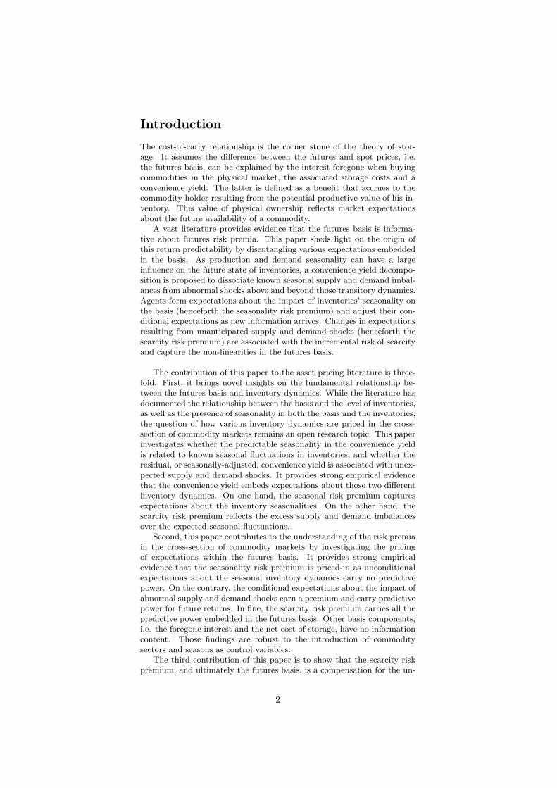
The cost-of-carry relationship is the corner stone of the theory of stor-age. It assumes the di˙erence between the futures and spot prices, i.e. the futures basis, can be explained by the interest foregone when buying commodities in the physical market, the associated storage costs and a convenience yield. The latter is defned as a beneft that accrues to the commodity holder resulting from the potential productive value of his in-ventory. This value of physical ownership refects market expectations about the future availability of a commodity.

A vast literature provides evidence that the futures basis is informa-tive about futures risk premia. This paper sheds light on the origin of this return predictability by disentangling various expectations embedded in the basis. As production and demand seasonality can have a large infuence on the future state of inventories, a convenience yield decompo-sition is proposed to dissociate known seasonal supply and demand imbal-ances from abnormal shocks above and beyond those transitory dynamics. Agents form expectations about the impact of inventories’ seasonality on the basis (henceforth the seasonality risk premium) and adjust their con-ditional expectations as new information arrives. Changes in expectations resulting from unanticipated supply and demand shocks (henceforth the scarcity risk premium) are associated with the incremental risk of scarcity and capture the non-linearities in the futures basis.

The contribution of this paper to the asset pricing literature is three-fold. First, it brings novel insights on the fundamental relationship be-tween the futures basis and inventory dynamics. While the literature has documented the relationship between the basis and the level of inventories, as well as the presence of seasonality in both the basis and the inventories, the question of how various inventory dynamics are priced in the cross-section of commodity markets remains an open research topic. This paper investigates whether the predictable seasonality in the convenience yield is related to known seasonal fuctuations in inventories, and whether the residual, or seasonally-adjusted, convenience yield is associated with unex-pected supply and demand shocks. It provides strong empirical evidence that the convenience yield embeds expectations about those two di˙erent inventory dynamics. On one hand, the seasonal risk premium captures expectations about the inventory seasonalities. On the other hand, the scarcity risk premium refects the excess supply and demand imbalances over the expected seasonal fuctuations.

Second, this paper contributes to the understanding of the risk premia in the cross-section of commodity markets by investigating the pricing of expectations within the futures basis. It provides strong empirical evidence that the seasonality risk premium is priced-in as unconditional expectations about the seasonal inventory dynamics carry no predictive power. On the contrary, the conditional expectations about the impact of abnormal supply and demand shocks earn a premium and carry predictive power for future returns. In fne, the scarcity risk premium carries all the predictive power embedded in the futures basis. Other basis components, i.e. the foregone interest and the net cost of storage, have no information content. Those fndings are robust to the introduction of commodity sectors and seasons as control variables.

The third contribution of this paper is to show that the scarcity risk premium, and ultimately the futures basis, is a compensation for the un-

2

expected increase in the risk of stock-out and that the associated return predictability fnds its origin in the slow di˙usion of information and un-derreaction to abnormal changes in inventories, above and beyond seasonal dynamics. It presents strong evidence of underreaction along the futures curve following a marginal change in the risk of stock-out. The under-reaction is broad based along the curve but more pronounced in the far contracts, leading to futures curve twists. These results suggest that mar-ket participants also underreact to the risk that the inventory depletion happens at faster rate than anticipated, as well as the risk that inventory imbalances might resorb at a lower speed than expected due to the slow adjustment of supply. Despite the slow di˙usion of information and the unexpected nature of the supply and demand shocks, information decays fast and the return predictability is transient. The diminishing statistical signifcance of excess returns with the length of the holding horizon indi-cates that the information is progressively di˙used throughout the market up until it is fully incorporated in futures prices. The scarcity risk pre-mium has signifcant predictive power up to a 3 months horizon, which is too short to be associated with a fundamental resolution of abnormal supply and demand imbalances.

This paper is organized as follows. Section 1 reviews the literature on the theory of storage and on the seasonality in commodity markets. Section 2 proposes a decomposition of the futures basis that disentangles expected seasonal shocks from unexpected shocks to inventories. Section 3 presents the data and methodologies used in this paper. Section 4 in-vestigates the fundamental relationship between the futures basis and the inventory dynamics. Section 5 provides empirical evidence on the pric-ing of expectations in the cross-section of commodity markets. The last section analyses the origins of the return predictability associated with the scarcity risk premium. To conclude, future avenues of research are discussed.

1 Literature review

The cost-of-carry relationship describes the no-arbitrage condition be-tween the spot and the futures price and defnes the futures basis. In commodity markets the traditional defntion is augmented by a term very specifc to perishable goods, the convenience yield. This value of physical ownership is the corner stone of the theory of storage and refects market expectations about the future availability of a commodity. More impor-tantly, the future basis has been found to be informative about futures risk premia. As production and demand seasonality can have a large infu-ence on the anticipations about the future state of inventories, this paper aims at shedding light on the origin of this predictability by disentangling various expectations embedded in the basis.

1.1 Theory of storage The theory of storage which fnds its foundation in the work of Kaldor (1939) and Working (1948) has been largely documented in the literature on commodity markets. Its corner stone, the cost-of-carry relationship,

3

assumes the di˙erence between futures prices and spot prices can be ex-plained by the interest foregone when buying commodities in the physical market, the associated storage costs and a convenience yield. The latter is defned as a beneft that accrues to the commodity holder resulting from the potential productive value of this inventory. Various model specifca-tion have been proposed in the literature to defne this cost-of-carry rela-tionship. Fama and French (1987) consider a model with fxed marginal storage cost and convenience yield. Szymanowska et al. (2014) propose an alternative defnition with proportional storage costs that accrues per period.

� � � � n n t t t (n) (n) (n)

F =St 1+RF 1+U −Ct+n

Ft (n) is the futures price at time t expiring in n-periods and St is the

spot price at time t. RFt (n) is the per-period risk-free rate at time t with

maturity t + n and known at t. Ut (n) is the per-period physical storage

costs, for storing commodities over n periods, expressed as a percentage of the spot price and known at t. Finally, the convenience yield Ct+n is defned as a cash payment occurring at time t + n and is also known in t.

The convenience yield can be interpreted as the net income, valued at time t, that the physical holder requires to sell his inventory at time t + n at the price Ft

(n) , once he has been compensated for the interest foregone and for the storage costs he is facing. Likewise, the convenience yield represents the net amount the futures investor is willing pay, beyond the current spot price St, i.e. the interest and storage costs compensation required by the commodity seller, in exchange for settling the purchase of the physical commodity at a price Ft

(n) . As such the convenience yield is foremost an implied quantity that rules out any arbitrage opportunity in the cost-of-carry model and describes the current equilibrium in futures markets.

A related concept is the futures basis which ties the current futures price Ft

(n) maturing in n periods to the current spot price St and summa-rizes the cost-of-carry relationship. The futures basis has also been coined the futures carry or roll-yield in the literature on commodities and is sim-ilar to other asset classes carry defnition.1 The below equation defnes the n-period log or percentage basis yt

(n) , i.e. the per-period futures carry for maturity n.

n o (n) (n)

F =St exp y ×nt t

Accordingly, the basis is a refection of the foregone interest, the stor-age costs and the convenience yield and can be directly estimated from observed futures and spot prices.

( )�� (n)n n(n) 1 (n) (n) Ct+n 1 F ty = ln 1+RF 1+U − = lnt n t t St n St

A large part of the literature on the theory of storage has focused on trying to model the dynamics of supply and demand that could explain the empirical distribution of commodity prices. Most commodities display non-normal distributions with high positive skewness and kurtosis, price

1Koijen et al. (2018) provide evidence of the presence of a carry factor across multiple asset classes.

4

jumps, non-linearities in prices and in conditional variance, as well as autocorrelation. The main hypothesis put forward to explain the behavior of prices are the inelasticity of demand in the presence of supply shocks with a non-linear functional form, the slow adjustment of supply and the lower boundaries on the level of inventories.

The impossibility to carry negative inventories plays a crucial role in the model of storage dynamics by Deaton and Laroque (1992) as it intro-duces the non-linearity able to characterize both the observed price jumps and conditional variance. Routledge et al. (2000) propose an equilibrium model for the commodity forward curve in which the non-negativity con-straint on inventory levels introduces an immediate consumption timing option in spot prices. The value of this option fuctuates with inventories and transitory shocks to supply and demand.

Gorton et al. (2013) provide the frst comprehensive study of the rela-tionship between physical inventories and commodity futures. They show that the shape of the futures curves is associated with the level of inven-tories and that this relationship becomes highly non-linear as the risk of a stock-out increases. This confrms the model predictions of Routledge et al. (2000) in which the elasticity of the convenience yield to changes in inventory levels is a decreasing function of inventory levels. Hevia et al. (2018) fnd that the non-linearity between inventories and commodity prices is negatively related to the maturity of the futures contract.

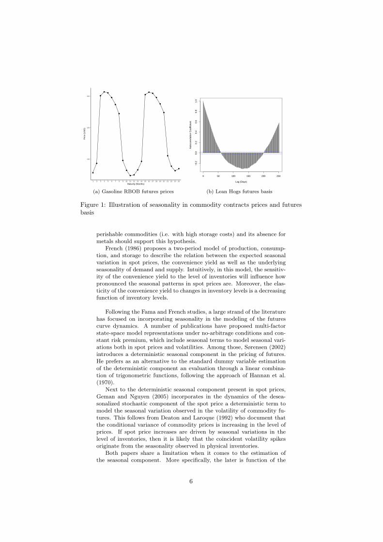
1.2 Seasonality Seasonality plays an important role in the theory of storage as both pro-duction and demand can exhibit seasonal patterns that impact inventories. The resulting inventory seasonality should infuence directly the conve-nience yield embedded in the basis and thus both the futures price and its carry. Figure 1 illustrates the presence of seasonality in both commodity futures prices as well as in the futures basis. Panel a of Figure 1 plots the futures curve of the Gasoline RBOB contract on 2016-01-05. Panel b of Figure 1 shows the autocorrelation coeÿcients of the futures basis in excess of the foregone interest for Lean Hogs futures contracts over 252 daily lags.

Finding support in the theory of storage and in the work of Brennan (1958) and Telser (1958) on the relationship between the convenience yield and the level of physical inventories, Fama and French (1987) test for the presence of seasonal variation in the basis using seasonal dummies. They fnd reliable evidence of seasonality in some agricultural and animal com-modities but none in metals. Moreover, they provide evidence that the basis has forecasting power for future spot changes of seasonal commodi-ties. More recently Brooks et al. (2013) have confrmed those fndings using a larger sample size and a broader universe of commodities. They provide additional robustness checks on the presence of seasonality in the basis and show that the forecasting power of the basis cannot be related to the magnitude of the seasonal patterns a commodity exhibits.

Fama and French (1987) argue that for commodities that exhibit sea-sonality in supply or demand, the predictability of future spot variation should be increasing in storage costs. Indeed, high costs should deter the build-up of inventories whose main function is to smooth demand and supply imbalances. The presence of forecasting power for some of the

5

●

●

●

●●

●

●

●

●

●

●●

●

●

●

●●

●

●

●

●

●

●

●

130

140

150

1 2 3 4 5 6 7 8 9 10 11 12 13 14 15 16 17 18 19 20 21 22 23 24

Maturity (Months)

Pric

e (U

SD

)

0 50 100 150 200 250

−0.

20.

00.

20.

40.

60.

81.

0

Lag (Days)

Aut

ocor

rela

tion

Coe

ffici

ent

(a) Gasoline RBOB futures prices (b) Lean Hogs futures basis

Figure 1: Illustration of seasonality in commodity contracts prices and futures basis

perishable commodities (i.e. with high storage costs) and its absence for metals should support this hypothesis.

French (1986) proposes a two-period model of production, consump-tion, and storage to describe the relation between the expected seasonal variation in spot prices, the convenience yield as well as the underlying seasonality of demand and supply. Intuitively, in this model, the sensitiv-ity of the convenience yield to the level of inventories will infuence how pronounced the seasonal patterns in spot prices are. Moreover, the elas-ticity of the convenience yield to changes in inventory levels is a decreasing function of inventory levels.

Following the Fama and French studies, a large strand of the literature has focused on incorporating seasonality in the modeling of the futures curve dynamics. A number of publications have proposed multi-factor state-space model representations under no-arbitrage conditions and con-stant risk premium, which include seasonal terms to model seasonal vari-ations both in spot prices and volatilities. Among those, Sørensen (2002) introduces a deterministic seasonal component in the pricing of futures. He prefers as an alternative to the standard dummy variable estimation of the deterministic component an evaluation through a linear combina-tion of trigonometric functions, following the approach of Hannan et al. (1970).

Next to the deterministic seasonal component present in spot prices, Geman and Nguyen (2005) incorporates in the dynamics of the desea-sonalized stochastic component of the spot price a deterministic term to model the seasonal variation observed in the volatility of commodity fu-tures. This follows from Deaton and Laroque (1992) who document that the conditional variance of commodity prices is increasing in the level of prices. If spot price increases are driven by seasonal variations in the level of inventories, then it is likely that the coincident volatility spikes originate from the seasonality observed in physical inventories.

Both papers share a limitation when it comes to the estimation of the seasonal component. More specifcally, the later is function of the

6

estimation date rather than of the maturity of the contract. Borovkova and Geman (2006) tackle this issue and consider a cost-of-carry model with a deterministic seasonal premium within a stochastic convenience yield. By relying on an average futures price along the curve, this approach does not disentangle the interest foregone from the seasonal component in the estimation.

More recently Hevia et al. (2018) develop a multi-factor aÿne model of commodity futures with stochastic seasonal fuctuations. In their nine factors approach, the seasonal shocks are driven by two unobserved fac-tors which only explain marginally the observed risk premia but still are non-negligible. Most of the risk premia originate from the spot factor and the three factors (i.e. level, slope, curvature) describing the cost-of-carry term structure. Interest rate factors’ infuence increases with the level of interest rate. Finally, the authors reveal the importance of allowing for time variation in the estimation of the seasonal component to match the time-variation of seasonal patterns observed in inventories. More impor-tantly this helps to avoid attributing erroneously those dynamics to other factors. The presence of non-linearities between inventories and the net convenience yield supports the theory of storage.

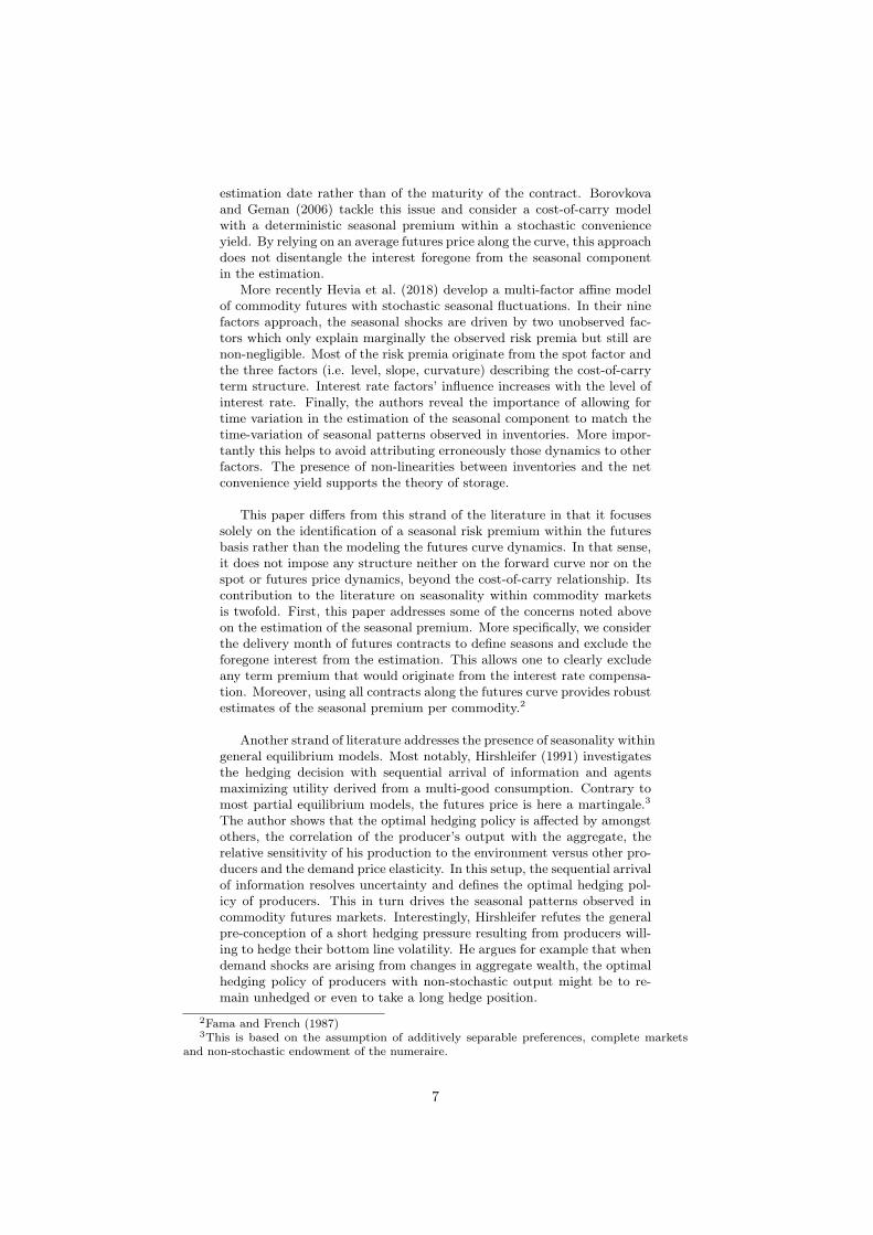
This paper di˙ers from this strand of the literature in that it focuses solely on the identifcation of a seasonal risk premium within the futures basis rather than the modeling the futures curve dynamics. In that sense, it does not impose any structure neither on the forward curve nor on the spot or futures price dynamics, beyond the cost-of-carry relationship. Its contribution to the literature on seasonality within commodity markets is twofold. First, this paper addresses some of the concerns noted above on the estimation of the seasonal premium. More specifcally, we consider the delivery month of futures contracts to defne seasons and exclude the foregone interest from the estimation. This allows one to clearly exclude any term premium that would originate from the interest rate compensa-tion. Moreover, using all contracts along the futures curve provides robust estimates of the seasonal premium per commodity.2

Another strand of literature addresses the presence of seasonality within general equilibrium models. Most notably, Hirshleifer (1991) investigates the hedging decision with sequential arrival of information and agents maximizing utility derived from a multi-good consumption. Contrary to most partial equilibrium models, the futures price is here a martingale.3

The author shows that the optimal hedging policy is a˙ected by amongst others, the correlation of the producer’s output with the aggregate, the relative sensitivity of his production to the environment versus other pro-ducers and the demand price elasticity. In this setup, the sequential arrival of information resolves uncertainty and defnes the optimal hedging pol-icy of producers. This in turn drives the seasonal patterns observed in commodity futures markets. Interestingly, Hirshleifer refutes the general pre-conception of a short hedging pressure resulting from producers will-ing to hedge their bottom line volatility. He argues for example that when demand shocks are arising from changes in aggregate wealth, the optimal hedging policy of producers with non-stochastic output might be to re-main unhedged or even to take a long hedge position.

2Fama and French (1987) 3This is based on the assumption of additively separable preferences, complete markets

and non-stochastic endowment of the numeraire.

7

Finally, a more recent strand of literature has focused on providing ev-idence of seasonality in returns across asset classes and of the proftability of the strategies aiming at exploiting these return dynamics.

Keloharju et al. (2016) document the presence of seasonality in returns across various stock portfolios and factors as well as in commodities using same month past returns as predictor. The authors investigate the source of the seasonality observed at the stock level. They suggest it could ei-ther emanate from the underlying risk factors’ seasonality, thus having a systematic origin, or resides within each individual security, being there-fore essentially of idiosyncratic nature. An alternative explanation to the recurrent variation in securities returns is that seasonality is merely the result of serial-correlation in innovations. Within stock markets, the au-thors fnd supportive evidence for the hypothesis that seasonality at the stock level is induced by their exposure to the underlying risk factors own seasonality. Finally, they show that return-based seasonal strategies are economically signifcant, cannot be explained by exposure to macroeco-nomic risks and are resilient to investors sentiment.

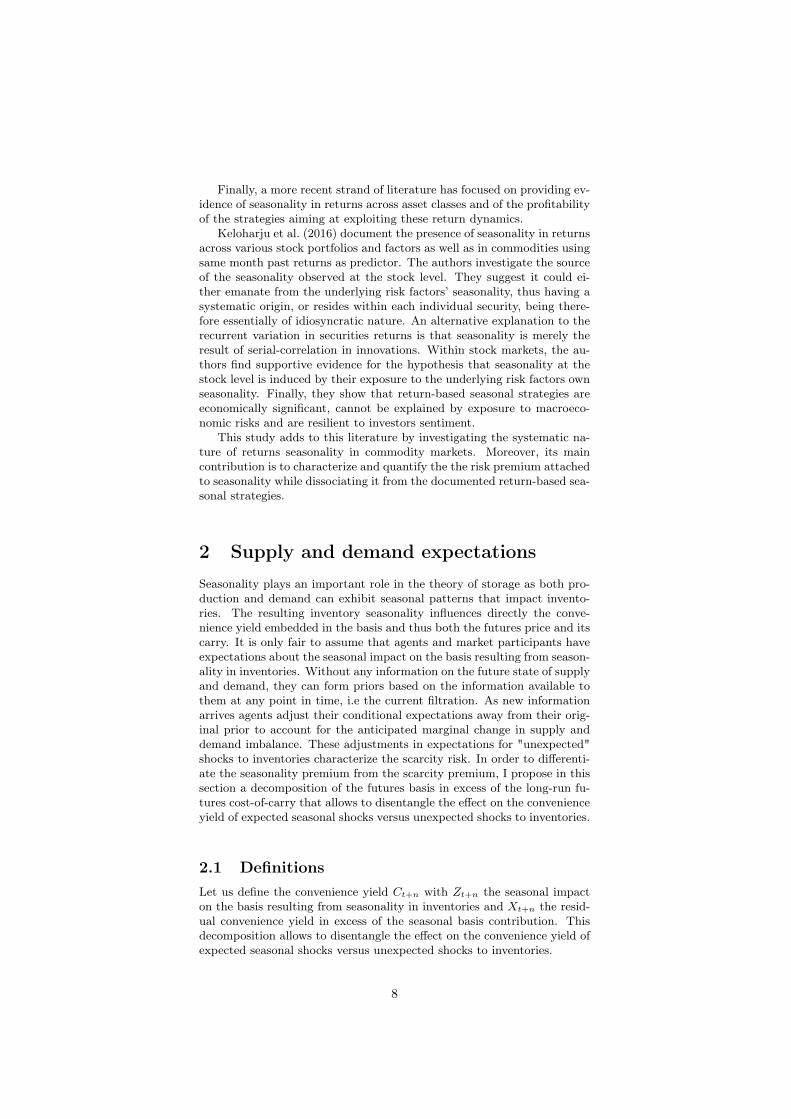
This study adds to this literature by investigating the systematic na-ture of returns seasonality in commodity markets. Moreover, its main contribution is to characterize and quantify the the risk premium attached to seasonality while dissociating it from the documented return-based sea-sonal strategies.

2 Supply and demand expectations

Seasonality plays an important role in the theory of storage as both pro-duction and demand can exhibit seasonal patterns that impact invento-ries. The resulting inventory seasonality infuences directly the conve-nience yield embedded in the basis and thus both the futures price and its carry. It is only fair to assume that agents and market participants have expectations about the seasonal impact on the basis resulting from season-ality in inventories. Without any information on the future state of supply and demand, they can form priors based on the information available to them at any point in time, i.e the current fltration. As new information arrives agents adjust their conditional expectations away from their orig-inal prior to account for the anticipated marginal change in supply and demand imbalance. These adjustments in expectations for "unexpected" shocks to inventories characterize the scarcity risk. In order to di˙erenti-ate the seasonality premium from the scarcity premium, I propose in this section a decomposition of the futures basis in excess of the long-run fu-tures cost-of-carry that allows to disentangle the e˙ect on the convenience yield of expected seasonal shocks versus unexpected shocks to inventories.

2.1 Defnitions Let us defne the convenience yield Ct+n with Zt+n the seasonal impact on the basis resulting from seasonality in inventories and Xt+n the resid-ual convenience yield in excess of the seasonal basis contribution. This decomposition allows to disentangle the e˙ect on the convenience yield of expected seasonal shocks versus unexpected shocks to inventories.

8

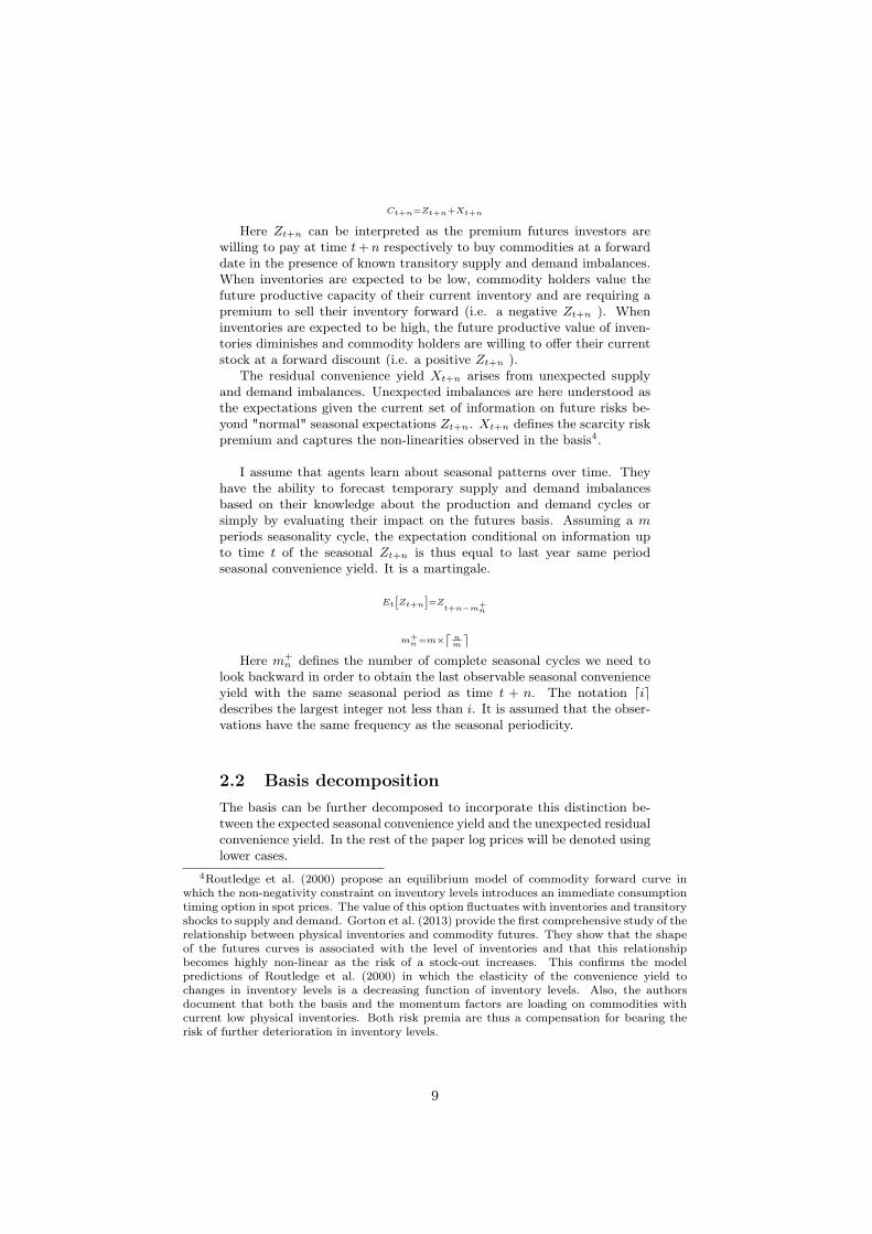
Ct+n =Zt+n+Xt+n

Here Zt+n can be interpreted as the premium futures investors are willing to pay at time t + n respectively to buy commodities at a forward date in the presence of known transitory supply and demand imbalances. When inventories are expected to be low, commodity holders value the future productive capacity of their current inventory and are requiring a premium to sell their inventory forward (i.e. a negative Zt+n ). When inventories are expected to be high, the future productive value of inven-tories diminishes and commodity holders are willing to o˙er their current stock at a forward discount (i.e. a positive Zt+n ).

The residual convenience yield Xt+n arises from unexpected supply and demand imbalances. Unexpected imbalances are here understood as the expectations given the current set of information on future risks be-yond "normal" seasonal expectations Zt+n. Xt+n defnes the scarcity risk premium and captures the non-linearities observed in the basis4 .

I assume that agents learn about seasonal patterns over time. They have the ability to forecast temporary supply and demand imbalances based on their knowledge about the production and demand cycles or simply by evaluating their impact on the futures basis. Assuming a m periods seasonality cycle, the expectation conditional on information up to time t of the seasonal Zt+n is thus equal to last year same period seasonal convenience yield. It is a martingale.

Et[Zt+n]=Z + t+n−mn

+ m =m×d n n m e

Here mn + defnes the number of complete seasonal cycles we need to

look backward in order to obtain the last observable seasonal convenience yield with the same seasonal period as time t + n. The notation die describes the largest integer not less than i. It is assumed that the obser-vations have the same frequency as the seasonal periodicity.

2.2 Basis decomposition The basis can be further decomposed to incorporate this distinction be-tween the expected seasonal convenience yield and the unexpected residual convenience yield. In the rest of the paper log prices will be denoted using lower cases.

4Routledge et al. (2000) propose an equilibrium model of commodity forward curve in which the non-negativity constraint on inventory levels introduces an immediate consumption timing option in spot prices. The value of this option fuctuates with inventories and transitory shocks to supply and demand. Gorton et al. (2013) provide the frst comprehensive study of the relationship between physical inventories and commodity futures. They show that the shape of the futures curves is associated with the level of inventories and that this relationship becomes highly non-linear as the risk of a stock-out increases. This confrms the model predictions of Routledge et al. (2000) in which the elasticity of the convenience yield to changes in inventory levels is a decreasing function of inventory levels. Also, the authors document that both the basis and the momentum factors are loading on commodities with current low physical inventories. Both risk premia are thus a compensation for bearing the risk of further deterioration in inventory levels.

9

�� Ct+n

St

n n(n) 1 (n) (n)y = ln 1+RF 1+U −t n t t

ln

⎧⎪⎨ ⎪⎩ ⎞ ⎟⎠ ⎫⎪⎬ ⎪⎭

⎛ ⎜⎝ �� Zt+n (n)

+Xt+n n n ��n n(n) (n)1

n St 1+RF

�1−1+RF 1+U=

=

t t (n)1+Ut t

ln

⎧⎪⎨ ⎪⎩ ⎫⎪⎬ ⎪⎭ Zt+n

(n)

+Xt+n n n ��(n) (n) 1

St 1+RF

�1−rf +u +t t (n)n 1+Ut t

The last term of the equation can be log-linearized following the ap-proach used by Campbell and Shiller (1988). I thus proceed to a frst-order Taylor series expansion around the long-run mean of both components of

¯ ¯the convenience yield, respectively Z and X.

ln

⎧⎪⎨ ⎪⎩ 1−

⎫⎪⎬ ⎪⎭ '

⎧⎪⎨ ⎪⎩ 1−

⎫⎪⎬ ⎪⎭ Zt+n (n)

+Xt+n n n �� Z+X

St 1+RF

� � �ln n n(n) (n) (n)1+U St 1+RF 1+U t t t t

��(Zt+n n n

St 1+RF 1+U −(Zt+n+Xt+n)(n) (n) t t

−X )� −Z)+(Xt+n�+

Furthermore, I impose a mild distributional restriction on the conve-nience yield by assuming its unconditional mean is zero. This assumption is easily met by detrending the convenience yield and requiring that any structural beneft the commodity owner might earn from physically hold-ing inventories is refected in a reduced net storage cost Ut

0(n) .

E[C]=0

Given the mean across seasons of an additive seasonal component is zero for a detrended series, the unconditional mean of Z is null.

P mEm[Z]= i=1 Zi=0

E[Z]=0

As a result, the unconditional mean of the residual convenience yield is also zero. Thus Xt+n captures the convenience yield resulting from transitory inventory imbalances arising from unexpected shocks in supply and demand.

E[X]=0

¯ ¯Assuming the long-run means Z and X equal their respective uncon-ditional mean, the log-linearization now simplifes to a sum of two terms, which are simply the proportions of the futures price that can be explained by respectively the seasonal component and the residual convenience yield.

ln

⎧⎪⎨ ⎪⎩ 1−

⎫⎪⎬ ⎪⎭ '− Zt+n (n)

��+Xt+n n n

Zt+n Xt+n� St 1+RF

−(n) (n)0(n) F F1+U t tt t

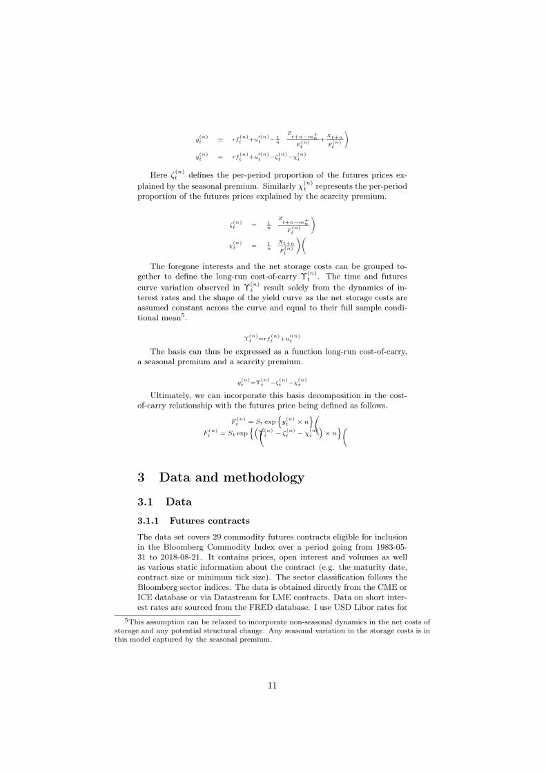
The per-period log-basis now simplifes to a linear equation with four terms capturing the foregone interests, the net storage costs, the seasonal premium and the residual convenience yield in excess of this seasonal component, i.e the scarcity premium.

10

!Z +

(n) (n) 0(n) t+n−mn Xt+n y ' rf +u − 1 +t t t n (n) (n)F F t t

(n) (n) 0(n) (n) (n)y = rf +u −ζ −χt t t t t

Here ζt (n) defnes the per-period proportion of the futures prices ex-

plained by the seasonal premium. Similarly χt (n) represents the per-period

proportion of the futures prices explained by the scarcity premium.

!Z

(n) 1 t+n−m + nζ = t n (n)

Ft ! (n) 1 Xt+nχ = t n (n)

F t

The foregone interests and the net storage costs can be grouped to-gether to defne the long-run cost-of-carry ( t

n) . The time and futures curve variation observed in t

(n) result solely from the dynamics of in-terest rates and the shape of the yield curve as the net storage costs are assumed constant across the curve and equal to their full sample condi-tional mean5 .

(n) (n) 0(n) =rf +ut t t

The basis can thus be expressed as a function long-run cost-of-carry, a seasonal premium and a scarcity premium.

(n) (n) (n) (n)y = −ζ −χt t t t

Ultimately, we can incorporate this basis decomposition in the cost-of-carry relationship with the futures price being defned as follows. n o

(n) (n)F = St exp y × nt tn� � o

(n) (n) (n) (n)F = St exp − ζ − χ × nt t t t

3 Data and methodology

3.1 Data

3.1.1 Futures contracts

The data set covers 29 commodity futures contracts eligible for inclusion in the Bloomberg Commodity Index over a period going from 1983-05-31 to 2018-08-21. It contains prices, open interest and volumes as well as various static information about the contract (e.g. the maturity date, contract size or minimum tick size). The sector classifcation follows the Bloomberg sector indices. The data is obtained directly from the CME or ICE database or via Datastream for LME contracts. Data on short inter-est rates are sourced from the FRED database. I use USD Libor rates for

5This assumption can be relaxed to incorporate non-seasonal dynamics in the net costs of storage and any potential structural change. Any seasonal variation in the storage costs is in this model captured by the seasonal premium.

11

maturities up to 1 year and interpolate with swap rates for longer matu-rities. Data for Libor rates and swap rates are available starting respec-tively on 1986-01-09 and 2000-07-03. Table A1 in Appendix A provides an overview of the di˙erent commodity markets, their sector classifcation, as well as the year of the frst futures contract.

Based on the set of available futures contracts, I create generic futures curves which allows to roll the futures contracts according to the desired rolling scheme. This allows to align the measurement of the signal based on the futures curve (e.g. the basis) with the desired implementation. For the purpose of this paper, futures contracts are rolled one day before the last trade date, defned as the minimum of the frst notice date, the last tradeable date and the last delivery date in order to accommodate varying contract specifcations across commodity futures.

This implementation di˙ers from the traditional approach followed in the literature which rolls futures contracts on the last day of the previ-ous month. This allows one to capture the dynamics of the scarcity risk up until it materializes. Indeed for contracts expiring close to month-end rolling at the beginning of the month would mean forgoing potentially valuable information about season specifc expectations of demand and supply imbalances.

Some commodities exhibit a non-regular contract cycle such that there might not be an outstanding contract for each season (e.g. there is only fve monthly contracts for wheat futures with delivery in March, May, July, September and December). To complement the set of available con-tracts, I create synthetic contracts to increase the breadth of the strategy. Upon data availability, these contracts are constructed by simple linear interpolation between a near and a far contract to obtain the desired ma-turity.

The futures exchange can issue two types of contract. On the one hand, most listed futures are issued for a subset of regular delivery months and constitute the contract cycle. On the other hand, the exchange can also issue serial contracts, which are "o˙" cycle. While the liquidity might be limited on serial contracts, it is diÿcult to identify those contracts through time as the choice by the exchanges of maturities up for issuance changes through time. Instead, to control for illiquidity, we handle the problem at the core and clean the data for stale pricing and impose a minimum number of pricing observations (set arbitrarily to 10).

3.1.2 Inventories

Physical inventories data for 27 commodities are collected from multiple exchanges, including the London Metal Exchange (LME), the Commod-ity Exchange (COMEX), the Intercontinental Exchange (ICE) and the New-York Mercantile Exchange (NYMEX), and governmental agencies, including the National Agricultural Statistics Services from the United States Department of Agriculture (NASS-USDA) and the United States Department of Energy (DOE). No inventory information is available for Brent Crude Oil. Table A2 in Appendix A provides an overview of the inventory data for each commodity market in our universe. It details the source, the starting year of the data, the reporting frequency and the re-porting lag applied to the series.

12

3.2 Basis decomposition

3.2.1 Estimation methodology

In the absence of reliable spot data and following the literature, the basis is measured between every consecutive contract along the futures curve starting from the frst active contract and is expressed in percent of the front contract price adjusted for the number of days until delivery in order to allow for a fair comparison across contracts with di˙erent maturities. Note that the term premium is defned from the second nearest contract and beyond this maturity.

The seasonal convenience yield is estimated by regression of a de-trended log-basis in excess of the foregone interest on seasonal dummies. Note that given the non-linearities observed in the basis, I use a robust regression methodology and the median is preferred to the mean for de-trending.

P(n) (n) 0(n) m y −rf −u = i=1 βt,idi+�tt t t

The restriction imposed on the unconditional mean of the convenience yield is enforced by setting the net storage cost ut

0(n) equal to the median of the log-basis in excess of the foregone interests v(n).

0(n) (n)u = vt

(n) (n) (n)v = y −rf t t t

The long-run cost-of-carry ( tn) is thus simplifed to incorporate this re-

striction while the two components of the convenience yield, i.e. the sea-sonal premium and the residual convenience yield in excess of the seasonal component, are defned as follows.

(n) (n) t (n) = rft + v P(n) mζt = − i=1 βt,idi

(n)χ = −�tt

I use a panel approach along the futures curve, i.e. considering all avail-able contracts at any point in time, and carry out the estimation on an expanding window to allow for the slow adjustment of expectations about the seasonal premium. The long-run net storage costs are estimated on the same measurement window as the seasonal convenience yield.

3.2.2 Full-sample estimates

Tables B1, B2, B3 and B4 in the Appendix show the full-sample estimates of the seasonal premium over the long-run cost-of-carry per commodity. The estimation has been carried out by means of robust regression using a panel approach along the futures curve, i.e. considering all available contracts at any point in time, using seasonal dummies. The results are reported using Newey-West standard errors, i.e. heteroskedasticity and

13

autocorrelation consistent estimate of the covariance matrix of the coeÿ-cient estimates.

Those results provide interesting insights on the heterogeneity of com-modities with regards to the seasonal risk premium and the infuence of time-variation in supply and demand. First, looking at the adjusted R2 of the regression allows to characterize the infuence of the seasonal factor as a driver of the futures basis. We see that highly seasonal commodities like natural gas (NG) have a R2 close to 0.6 while for aluminum this number is barely di˙erent from zero. The more pronounced the seasonal variations are, i.e. the amplitude of the premium across seasons, the higher the ad-justed R2 of the regression as they are large contributors to the variance of the basis. This is thus a useful indicator to classify commodities as seasonal or non-seasonal commodities.

Second, the estimated premia per season are usually highly statisti-cally signifcant, i.e. at the 1% confdence level, for seasonal commodities. Non-seasonal commodities like platinum (PL) can also have specifc sea-sons with a statistically signifcant premium. While the alternative and equivalent trigonometric approach6 to estimating seasonal components is convenient to understand the components of the seasonal cycle, the chosen simple dummy regression approach suÿces in characterizing the premium attached to futures contract maturing in specifc seasons.

3.2.3 Futures curve decomposition

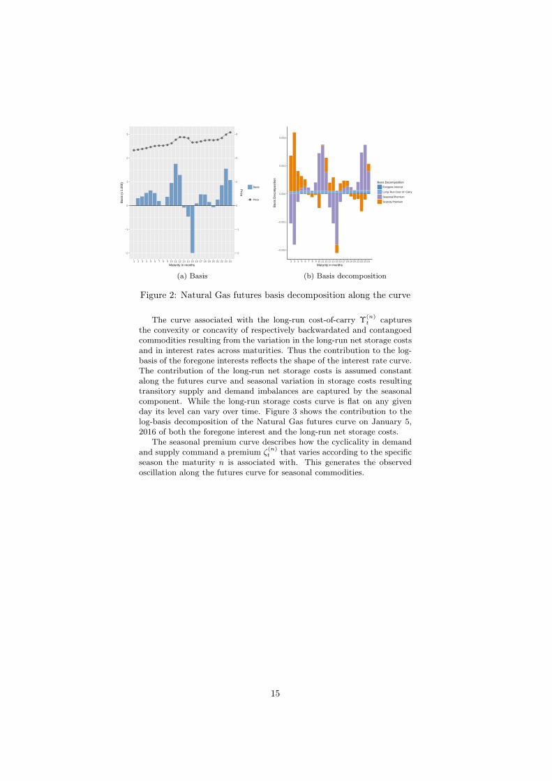
The basis measured over various investment horizons n fully describes the shape of the futures curve. Alternatively measuring the basis between every subsequent futures along the curve delivers an equivalent representa-tion.7 Given the above basis decomposition, we can assess how the time to maturity infuences each component independently along the curve. For illustration purpose, Figure 2 shows the log-basis decomposition of the Natural Gas futures curve on January 5, 2016 when measured from consecutive contracts.

6See, for example, Hannan et al. (1970), Sørensen (2002), Borovkova and Geman (2006) or Hevia et al. (2018) for more details on the trigonometric specifcation of seasonality. The results indicate the need to tailor the inclusion of the harmonics beyond the fundamental frequency to di˙erentiate between commodities.

7Such a representation is conceptually similar to the notion of forward rates along fxed income yield curves.

14

● ● ● ● ● ● ● ● ●●

●● ● ●

● ● ● ● ● ● ●●

●●

−2

−1

0

1

2

3

−2

−1

0

1

2

3

1 2 3 4 5 6 7 8 9 10 11 12 13 14 15 16 17 18 19 20 21 22 23 24

Maturity in months

Bas

is (

x 1.

000)

Price

Basis

● Price

−0.002

−0.001

0.000

0.001

0.002

2 3 4 5 6 7 8 9 10 11 12 13 14 15 16 17 18 19 20 21 22 23 24

Maturity in months

Bas

is D

ecom

posi

tion

Basis Decomposition

Foregone Interest

Long−Run Cost−of−Carry

Seasonal Premium

Scarcity Premium

(a) Basis (b) Basis decomposition

Figure 2: Natural Gas futures basis decomposition along the curve

The curve associated with the long-run cost-of-carry ( tn) captures

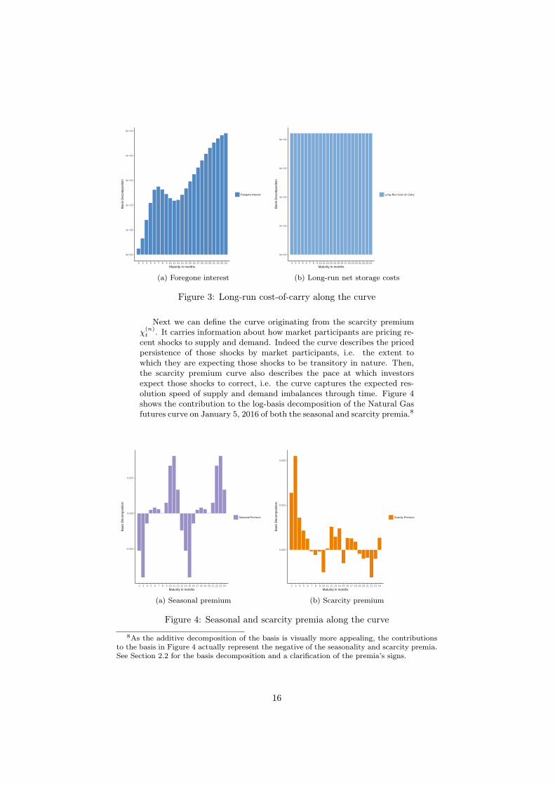
the convexity or concavity of respectively backwardated and contangoed commodities resulting from the variation in the long-run net storage costs and in interest rates across maturities. Thus the contribution to the log-basis of the foregone interests refects the shape of the interest rate curve. The contribution of the long-run net storage costs is assumed constant along the futures curve and seasonal variation in storage costs resulting transitory supply and demand imbalances are captured by the seasonal component. While the long-run storage costs curve is fat on any given day its level can vary over time. Figure 3 shows the contribution to the log-basis decomposition of the Natural Gas futures curve on January 5, 2016 of both the foregone interest and the long-run net storage costs.

The seasonal premium curve describes how the cyclicality in demand and supply command a premium ζt

(n) that varies according to the specifc season the maturity n is associated with. This generates the observed oscillation along the futures curve for seasonal commodities.

15

0e+00

1e−05

2e−05

3e−05

4e−05

5e−05

2 3 4 5 6 7 8 9 10 11 12 13 14 15 16 17 18 19 20 21 22 23 24

Maturity in months

Bas

is D

ecom

posi

tion

Foregone Interest

0e+00

2e−05

4e−05

6e−05

8e−05

2 3 4 5 6 7 8 9 10 11 12 13 14 15 16 17 18 19 20 21 22 23 24

Maturity in months

Bas

is D

ecom

posi

tion

Long−Run Cost−of−Carry

(a) Foregone interest (b) Long-run net storage costs

Figure 3: Long-run cost-of-carry along the curve

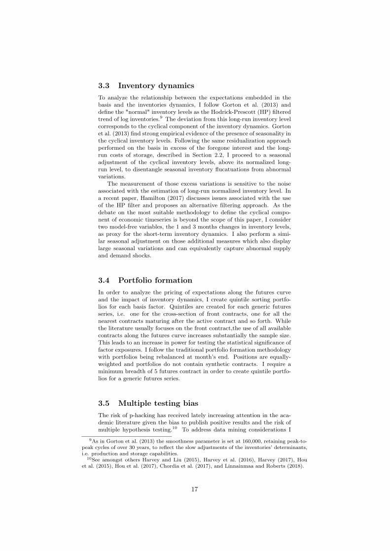
Next we can defne the curve originating from the scarcity premium χt (n) . It carries information about how market participants are pricing re-

cent shocks to supply and demand. Indeed the curve describes the priced persistence of those shocks by market participants, i.e. the extent to which they are expecting those shocks to be transitory in nature. Then, the scarcity premium curve also describes the pace at which investors expect those shocks to correct, i.e. the curve captures the expected res-olution speed of supply and demand imbalances through time. Figure 4 shows the contribution to the log-basis decomposition of the Natural Gas futures curve on January 5, 2016 of both the seasonal and scarcity premia.8

−0.001

0.000

0.001

2 3 4 5 6 7 8 9 10 11 12 13 14 15 16 17 18 19 20 21 22 23 24

Maturity in months

Bas

is D

ecom

posi

tion

Seasonal Premium

0.000

0.001

0.002

2 3 4 5 6 7 8 9 10 11 12 13 14 15 16 17 18 19 20 21 22 23 24

Maturity in months

Bas

is D

ecom

posi

tion

Scarcity Premium

(a) Seasonal premium (b) Scarcity premium

Figure 4: Seasonal and scarcity premia along the curve

8As the additive decomposition of the basis is visually more appealing, the contributions to the basis in Figure 4 actually represent the negative of the seasonality and scarcity premia. See Section 2.2 for the basis decomposition and a clarifcation of the premia’s signs.

16

3.3 Inventory dynamics To analyze the relationship between the expectations embedded in the basis and the inventories dynamics, I follow Gorton et al. (2013) and defne the "normal" inventory levels as the Hodrick-Prescott (HP) fltered trend of log inventories.9 The deviation from this long-run inventory level corresponds to the cyclical component of the inventory dynamics. Gorton et al. (2013) fnd strong empirical evidence of the presence of seasonality in the cyclical inventory levels. Following the same residualization approach performed on the basis in excess of the foregone interest and the long-run costs of storage, described in Section 2.2, I proceed to a seasonal adjustment of the cyclical inventory levels, above its normalized long-run level, to disentangle seasonal inventory fucatuations from abnormal variations.

The measurement of those excess variations is sensitive to the noise associated with the estimation of long-run normalized inventory level. In a recent paper, Hamilton (2017) discusses issues associated with the use of the HP flter and proposes an alternative fltering approach. As the debate on the most suitable methodology to defne the cyclical compo-nent of economic timeseries is beyond the scope of this paper, I consider two model-free variables, the 1 and 3 months changes in inventory levels, as proxy for the short-term inventory dynamics. I also perform a simi-lar seasonal adjustment on those additional measures which also display large seasonal variations and can equivalently capture abnormal supply and demand shocks.

3.4 Portfolio formation In order to analyze the pricing of expectations along the futures curve and the impact of inventory dynamics, I create quintile sorting portfo-lios for each basis factor. Quintiles are created for each generic futures series, i.e. one for the cross-section of front contracts, one for all the nearest contracts maturing after the active contract and so forth. While the literature usually focuses on the front contract,the use of all available contracts along the futures curve increases substantially the sample size. This leads to an increase in power for testing the statistical signifcance of factor exposures. I follow the traditional portfolio formation methodology with portfolios being rebalanced at month’s end. Positions are equally-weighted and portfolios do not contain synthetic contracts. I require a minimum breadth of 5 futures contract in order to create quintile portfo-lios for a generic futures series.

3.5 Multiple testing bias The risk of p-hacking has received lately increasing attention in the aca-demic literature given the bias to publish positive results and the risk of multiple hypothesis testing.10 To address data mining considerations I

9As in Gorton et al. (2013) the smoothness parameter is set at 160,000, retaining peak-to-peak cycles of over 30 years, to refect the slow adjustments of the inventories’ determinants, i.e. production and storage capabilities.

10See amongst others Harvey and Liu (2015), Harvey et al. (2016), Harvey (2017), Hou et al. (2015), Hou et al. (2017), Chordia et al. (2017), and Linnainmaa and Roberts (2018).

17

follow the recommendation of Harvey et al. (2016) to raise the statistical signifcance threshold and reject the null hypothesis for t-statistics above 3.0.

4 Fundamental expectations

So far I have suggested that the basis decomposition proposed in Section 2.2 allows to disentangle unconditional expectations about the seasonal impact on the basis, resulting from known seasonality in inventories, from conditional expectations originating from abnormal shocks to inventories that characterize the scarcity risk. Without any information on the future state of supply and demand, market participants form priors based on the information available to them at any point in time, i.e the current fltration, and as new information arrives agents adjust their conditional expectations away from their original priors to account for the anticipated marginal change in supply and demand imbalance.

In this section, I investigate the fundamental nature of the expecta-tions built-in the convenience yield. More specifcally, I test the associated hypotheses that the seasonal premium is driven by the seasonality of in-ventories while the scarcity premium originates from the excess inventory dynamics. For a robust evaluation of those relationships, I conduct panel regression and a sorting portfolio exposure analysis using three proxies of the inventory dynamics.

4.1 Panel regressions To analyze the non-linear relationship between the basis and inventories Gorton et al. (2013) estimate a cubic spline regression of the basis on normalized inventory levels, i.e. detrended using a Hodrick-Prescott (HP) flter to capture the lon-run inventory level, and account for seasonal vari-ations in the basis using dummy variables. While the authors provide strong evidence of this non-linear relationship, their model specifcation does not allow to dissociate the e˙ect of prior expectations, originating from known seasonal variations in supply and demand, from marginal adjustment resulting from fundamental abnormal shocks. Indeed, the normalized inventory level is not seasonally-adjusted in their approach al-though they fnd strong empirical evidence of the presence of seasonality in inventories.

To specifcally analyze the infuence of inventory seasonality and ab-normal supply and demand shocks, I conduct panel regressions of the basis, as well as for each of its components, on those inventory dynamics. As in the vast majority of cases, the Hausman (1978) test supports the use of random e˙ects, they are systematically controlled for in the estimation. The analysis is conducted on month-end data for the front contract and the results are robust to the use of daily data. The t-statistics rely on the heteroskedasticity and autocorrelation consistent Newey and West (1987) standard errors estimates, using the Newey and West (1994) automatic lag selection procedure. The results for the univariate regressions on the level of the three inventory dynamics proxies are reported in Appendix C.

Table 1 presents the results when the estimation is conducted on the cyclical inventory level components. We see that the basis is signifcantly

18

exposed to the abnormal cyclical inventory level in excess of its seasonal component. This exposure originates from the scarcity premium which exhibits a similar exposure and thus confrms the hypothesis.

Table 1: Regression basis factors on inventory cycle components.

Intercept Basis 0.0001

t = 3.130 ∗∗∗

ForegoneInt 0.00004

t = 20.108 ∗∗∗

Median −0.00004

t = −2.132 ∗∗

Season 0.00002

t = 1.165

Scarcity 0.0001

t = 3.143 ∗∗∗

Inv Cycle Season −0.0003 t = −1.466

−0.00001 t = −3.225 ∗∗∗

0.00001 t = 2.549 ∗∗

−0.0004 t = −2.339 ∗∗

0.0001 t = 0.421

Inv Cycle Excess 0.0003 t = 4.235 ∗∗∗

−0.00001 t = −1.065

0.00001 t = 2.075 ∗∗

0.00004 t = 2.843 ∗∗∗

0.0003 t = 4.298 ∗∗∗

Adjusted R2 0.026 0.002 0.005 0.026 0.027

Note: The t-statistics rely on the heteroskedasticity and autocorrelation consistent Newey-West (1987) standard errors estimates, using the Newey-West (1994) automatic lag selection procedure. *p<0.1; **p<0.05; ***p<0.01

Interestingly, the seasonal premium has a negative exposure to the sea-sonal component of the cyclical inventory level. The diÿculty associated with the interpretation of those results is that the cyclical inventory sea-sonal component is a level metric while the basis is a change measure, here defned as the di˙erence between the futures contract and the spot prices. As such while a positive seasonal inventory component is expected to lead to a relatively lower spot price and higher basis all else equal, implying a positive relationship, this measure abstracts from the expected seasonal component associated with the futures contract and thus a˙ects the basis. If the futures curve captures the seasonality of inventories, prices along the curve should be a refection of the seasonal inventory level, implying in a negative relationship. The positive relationship of the seasonal pre-mium with the excess inventory level is more diÿcult to interpret. Indeed, it could suggest that the excess and seasonals component of the cyclical inventory level are correlated although they should be orthogonal by de-sign. I confrmed ex-post that two components are independant with a close to null correlation. In light of the ten times lower coeÿcient for the excess inventory level, I conclude this is a second order e˙ect.

Table 2: Regression basis factors on 3 months inventory changes.


t = 3.158 ∗∗∗

ForegoneInt 0.00004

t = 19.971 ∗∗∗

Median −0.00004

t = −2.128 ∗∗

Season 0.00002

t = 1.048

Scarcity 0.0001

t = 3.133 ∗∗∗

Inv Chg 3M Season 0.004 t = 1.533

−0.00001 t = −0.414

−0.00001 t = −0.317

0.002 t = 1.420

0.002 t = 1.545

Inv Chg 3M Excess 0.001 t = 1.762 ∗

0.00001 t = 0.763

−0.0001 t = −2.072 ∗∗

0.0001 t = 0.337

0.001 t = 2.351 ∗∗

Adjusted R2 0.013 -0.0002 0.002 0.011 0.007


Table 2 and Table 3 present the results when the estimation is con-ducted on the components of respectively the 3 months and 1 month change in inventories. In both tables we can see a similar pattern emerging with the basis and the scarcity premium having a statistically signifcant exposure to the excess inventory changes, while the seasonal premium is loading, although not signifcantly, on the seasonal component of those changes.

19

Table 3: Regression basis factors on 1 month inventory changes.


t = 3.143 ∗∗∗

ForegoneInt 0.00004

t = 19.969 ∗∗∗

Median −0.00004

t = −2.128 ∗∗

Season 0.00002

t = 1.109

Scarcity 0.0001

t = 3.123 ∗∗∗

Inv Chg 1M Season 0.009 t = 1.596

0.00000 t = 0.017

−0.00004 t = −0.600

0.007 t = 1.740 ∗

0.002 t = 0.890

Inv Chg 1M Excess 0.001 t = 1.816 ∗

0.00000 t = 0.260

−0.0001 t = −1.822 ∗

0.0002 t = 0.630

0.001 t = 2.645 ∗∗∗

Adjusted R2 0.012 -0.0001 0.0002 0.027 0.001


4.2 Sorting portfolio exposures To provide further insights on the infuence of inventory dynamics on the basis and its components, this section investigates, for each basis compo-nent, the sorting portfolios exposure to inventory characteristics. Table 4 provides information on the results of this non-parametric approach. The average exposure to all three inventory dynamics proxies, in terms of level and its seasonal and abnormal components, is reported for each quintile portfolio. For each basis factor, the last row contains the t-statistic for the di˙erence in mean exposure between the top and bottom portfolios. The t-statistics above 3.0 are shown in bold and the asterisk identifes the characteristics for which the quintiles also display a monotonic behavior.

We observe for the basis portfolios signifcant di˙erences in exposures to the excess cyclical inventory level and the 1 month inventory change between the top and bottom portfolios. The seasonal premium portfolios have highly signifcant exposure to the level and seasonal component of both the 1 month and 3 months inventory changes. The scarcity pre-mium has signifcant exposure to all level and excess components of all three proxies for inventory dynamics.

Those results add to the literature. First, they bring additional em-pirical evidence on the relationship between the futures basis and the in-ventory dynamics in the cross-section of commodity markets. The second and more relevant contribution is to provide robust support to the claim that the basis embeds expectations about two di˙erent inventory dynam-ics. On one hand, the seasonal premium captures expectations about the cross-sectional dispersion in inventory seasonalities. On the other hand, the scarcity premium refects the excess supply and demand imbalances over the expected seasonal fuctuations.

20

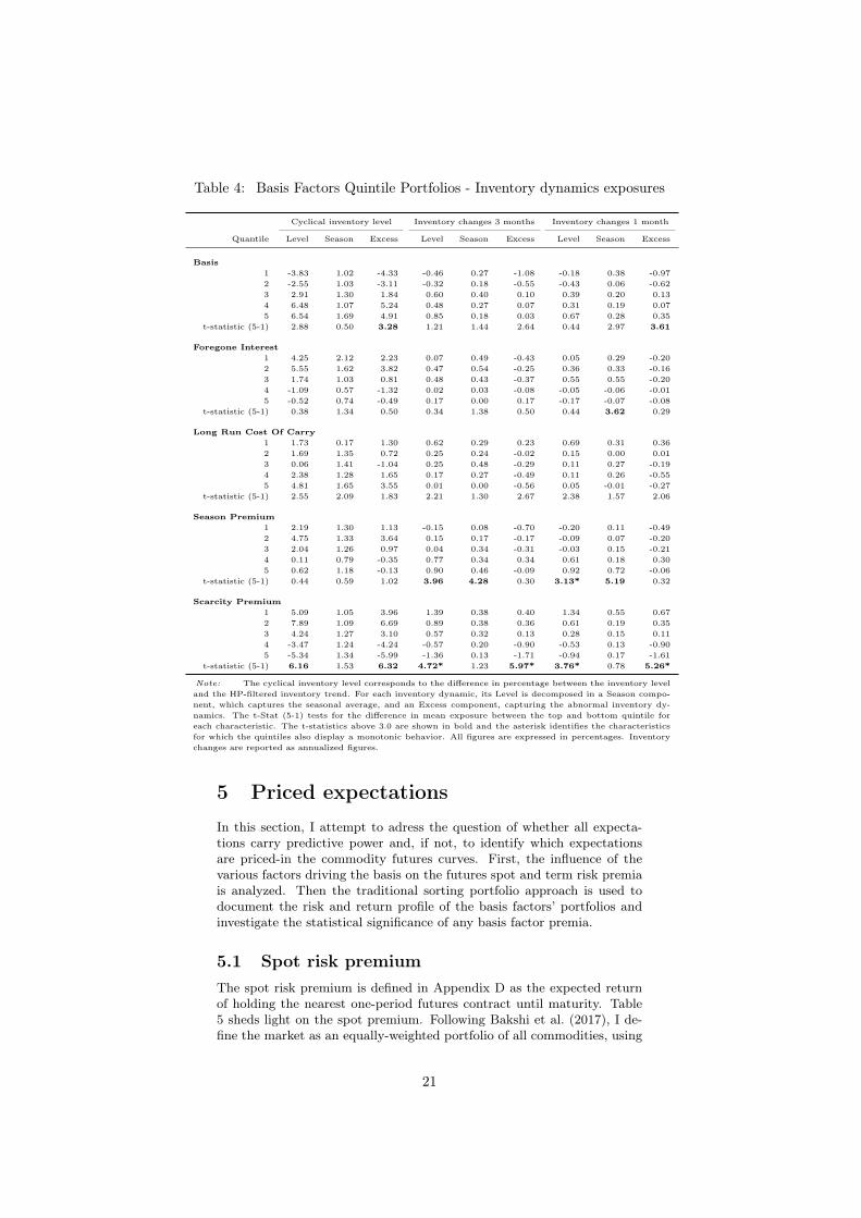
Table 4: Basis Factors Quintile Portfolios - Inventory dynamics exposures

Cyclical inventory level Inventory changes 3 months Inventory changes 1 month

Quantile Level Season Excess Level Season Excess Level Season Excess

Basis 1 -3.83 1.02 -4.33 -0.46 0.27 -1.08 -0.18 0.38 -0.97 2 -2.55 1.03 -3.11 -0.32 0.18 -0.55 -0.43 0.06 -0.62 3 2.91 1.30 1.84 0.60 0.40 0.10 0.39 0.20 0.13 4 6.48 1.07 5.24 0.48 0.27 0.07 0.31 0.19 0.07 5 6.54 1.69 4.91 0.85 0.18 0.03 0.67 0.28 0.35

t-statistic (5-1) 2.88 0.50 3.28 1.21 1.44 2.64 0.44 2.97 3.61

Foregone Interest 1 4.25 2.12 2.23 0.07 0.49 -0.43 0.05 0.29 -0.20 2 5.55 1.62 3.82 0.47 0.54 -0.25 0.36 0.33 -0.16 3 1.74 1.03 0.81 0.48 0.43 -0.37 0.55 0.55 -0.20 4 -1.09 0.57 -1.32 0.02 0.03 -0.08 -0.05 -0.06 -0.01 5 -0.52 0.74 -0.49 0.17 0.00 0.17 -0.17 -0.07 -0.08

t-statistic (5-1) 0.38 1.34 0.50 0.34 1.38 0.50 0.44 3.62 0.29

Long Run Cost Of Carry 1 1.73 0.17 1.30 0.62 0.29 0.23 0.69 0.31 0.36 2 1.69 1.35 0.72 0.25 0.24 -0.02 0.15 0.00 0.01 3 0.06 1.41 -1.04 0.25 0.48 -0.29 0.11 0.27 -0.19 4 2.38 1.28 1.65 0.17 0.27 -0.49 0.11 0.26 -0.55 5 4.81 1.65 3.55 0.01 0.00 -0.56 0.05 -0.01 -0.27

t-statistic (5-1) 2.55 2.09 1.83 2.21 1.30 2.67 2.38 1.57 2.06

Season Premium 1 2.19 1.30 1.13 -0.15 0.08 -0.70 -0.20 0.11 -0.49 2 4.75 1.33 3.64 0.15 0.17 -0.17 -0.09 0.07 -0.20 3 2.04 1.26 0.97 0.04 0.34 -0.31 -0.03 0.15 -0.21 4 0.11 0.79 -0.35 0.77 0.34 0.34 0.61 0.18 0.30 5 0.62 1.18 -0.13 0.90 0.46 -0.09 0.92 0.72 -0.06

t-statistic (5-1) 0.44 0.59 1.02 3.96 4.28 0.30 3.13* 5.19 0.32

Scarcity Premium 1 5.09 1.05 3.96 1.39 0.38 0.40 1.34 0.55 0.67 2 7.89 1.09 6.69 0.89 0.38 0.36 0.61 0.19 0.35 3 4.24 1.27 3.10 0.57 0.32 0.13 0.28 0.15 0.11 4 -3.47 1.24 -4.24 -0.57 0.20 -0.90 -0.53 0.13 -0.90 5 -5.34 1.34 -5.99 -1.36 0.13 -1.71 -0.94 0.17 -1.61

t-statistic (5-1) 6.16 1.53 6.32 4.72* 1.23 5.97* 3.76* 0.78 5.26*

Note: The cyclical inventory level corresponds to the di˙erence in percentage between the inventory level and the HP-fltered inventory trend. For each inventory dynamic, its Level is decomposed in a Season compo-nent, which captures the seasonal average, and an Excess component, capturing the abnormal inventory dy-namics. The t-Stat (5-1) tests for the di˙erence in mean exposure between the top and bottom quintile for each characteristic. The t-statistics above 3.0 are shown in bold and the asterisk identifes the characteristics for which the quintiles also display a monotonic behavior. All fgures are expressed in percentages. Inventory changes are reported as annualized fgures.

5 Priced expectations

In this section, I attempt to adress the question of whether all expecta-tions carry predictive power and, if not, to identify which expectations are priced-in the commodity futures curves. First, the infuence of the various factors driving the basis on the futures spot and term risk premia is analyzed. Then the traditional sorting portfolio approach is used to document the risk and return profle of the basis factors’ portfolios and investigate the statistical signifcance of any basis factor premia.

5.1 Spot risk premium The spot risk premium is defned in Appendix D as the expected return of holding the nearest one-period futures contract until maturity. Table 5 sheds light on the spot premium. Following Bakshi et al. (2017), I de-fne the market as an equally-weighted portfolio of all commodities, using

21

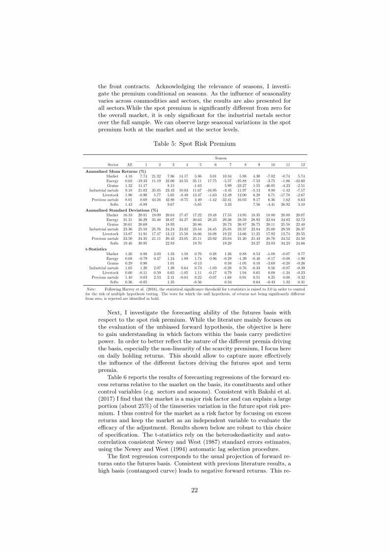
the front contracts. Acknowledging the relevance of seasons, I investi-gate the premium conditional on seasons. As the infuence of seasonality varies across commodities and sectors, the results are also presented for all sectors.While the spot premium is signifcantly di˙erent from zero for the overall market, it is only signifcant for the industrial metals sector over the full sample. We can observe large seasonal variations in the spot premium both at the market and at the sector levels.

Table 5: Spot Risk Premium

Season

Sector All 1 2 3 4 5 6 7 8 9 10 11 12

Annualized Mean Returns (%) Market 4.16 7.74 21.32 7.86 14.17 5.86 3.01 10.34 5.98 4.30 -7.82 -0.74 5.74 Energy 0.62 -19.33 11.19 32.06 42.55 35.11 17.75 -5.57 -25.88 -7.52 -3.75 -1.86 -42.60 Grains 1.32 11.17 8.15 -1.63 5.99 -23.27 1.55 -46.85 -4.23 -2.51

Industrial metals 9.18 21.02 35.85 23.43 10.03 11.67 -16.95 -3.45 11.97 -5.13 9.80 -1.42 -7.17 Livestock 1.96 -0.90 5.77 5.05 -8.49 13.47 -1.63 12.49 12.00 6.28 0.71 -17.78 -2.67

Precious metals 8.01 0.68 44.24 42.80 -0.75 4.49 -1.42 -32.41 16.03 9.17 6.36 1.62 6.63 Softs 1.43 -0.89 9.67 -5.65 3.33 7.56 -4.41 26.92 3.10

Annualized Standard Deviations (%) Market 16.33 20.81 19.09 20.04 17.47 17.22 19.48 17.55 14.95 18.35 18.80 20.88 20.07 Energy 31.31 36.29 35.48 38.07 34.27 30.63 28.23 29.36 28.59 28.92 32.84 34.83 32.72 Grains 20.61 20.69 18.93 20.86 20.73 26.87 26.75 20.11 25.58 22.40

Industrial metals 23.36 25.58 25.76 24.24 23.02 23.44 24.45 25.05 23.37 22.84 25.00 29.59 26.37 Livestock 13.87 14.91 17.47 13.12 15.58 16.66 16.08 19.22 13.66 11.25 17.92 12.74 20.55

Precious metals 23.50 24.35 21.11 20.43 23.05 25.11 23.92 23.04 21.20 21.43 28.70 24.52 24.50 Softs 19.46 30.95 22.83 19.70 19.20 23.27 23.83 34.23 24.66

t-Statistics Market 1.26 0.80 2.03 1.33 1.58 0.76 0.28 1.26 0.88 0.53 -1.08 -0.07 0.77 Energy 0.08 -0.79 0.47 1.24 1.89 1.74 0.96 -0.29 -1.39 -0.40 -0.17 -0.08 -1.90 Grains 0.29 0.90 1.01 -0.13 0.50 -1.05 0.10 -2.69 -0.28 -0.26

Industrial metals 1.65 1.20 2.07 1.39 0.64 0.73 -1.03 -0.20 0.76 -0.33 0.56 -0.07 -0.39 Livestock 0.60 -0.11 0.59 0.65 -1.05 1.11 -0.17 0.79 1.94 0.65 0.08 -1.34 -0.23

Precious metals 1.40 0.03 2.53 2.41 -0.04 0.22 -0.07 -1.68 0.91 0.51 0.25 0.08 0.32 Softs 0.36 -0.05 1.35 -0.56 0.34 0.64 -0.43 1.32 0.31

Note: Following Harvey et al. (2016), the statistical signifcance threshold for t-statistics is raised to 3.0 in order to control for the risk of multiple hypothesis testing. The tests for which the null hypothesis, of returns not being signifcantly di˙erent from zero, is rejected are identifed in bold.

Next, I investigate the forecasting ability of the futures basis with respect to the spot risk premium. While the literature mainly focuses on the evaluation of the unbiased forward hypothesis, the objective is here to gain understanding in which factors within the basis carry predictive power. In order to better refect the nature of the di˙erent premia driving the basis, especially the non-linearity of the scarcity premium, I focus here on daily holding returns. This should allow to capture more e˙ectively the infuence of the di˙erent factors driving the futures spot and term premia.

Table 6 reports the results of forecasting regressions of the forward ex-cess returns relative to the market on the basis, its constituents and other control variables (e.g. sectors and seasons). Consistent with Bakshi et al. (2017) I fnd that the market is a major risk factor and can explain a large portion (about 25%) of the timeseries variation in the future spot risk pre-mium. I thus control for the market as a risk factor by focusing on excess returns and keep the market as an independent variable to evaluate the eÿcacy of the adjustment. Results shown below are robust to this choice of specifcation. The t-statistics rely on the heteroskedasticity and auto-correlation consistent Newey and West (1987) standard errors estimates, using the Newey and West (1994) automatic lag selection procedure.

The frst regression corresponds to the usual projection of forward re-turns onto the futures basis. Consistent with previous literature results, a high basis (contangoed curve) leads to negative forward returns. This re-

22

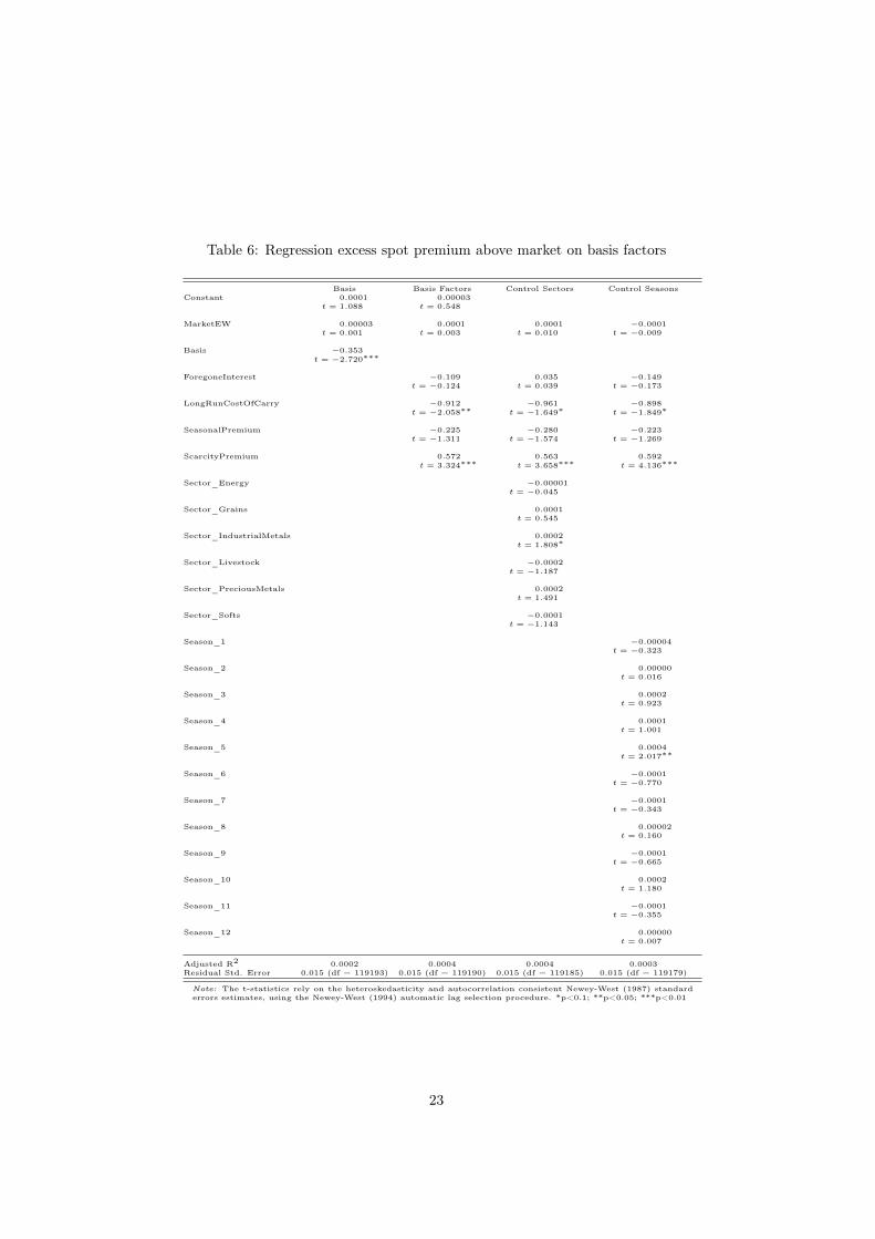
Table 6: Regression excess spot premium above market on basis factors

Constant Basis 0.0001

t = 1.088

Basis Factors 0.00003

t = 0.548

Control Sectors Control Seasons

MarketEW 0.00003 t = 0.001

0.0001 t = 0.003

0.0001 t = 0.010

−0.0001 t = −0.009

Basis −0.353 t = −2.720 ∗∗∗

ForegoneInterest −0.109 t = −0.124

0.035 t = 0.039

−0.149 t = −0.173

LongRunCostOfCarry −0.912 t = −2.058 ∗∗

−0.961 t = −1.649 ∗

−0.898 t = −1.849 ∗

SeasonalPremium −0.225 t = −1.311

−0.280 t = −1.574

−0.223 t = −1.269

ScarcityPremium 0.572 t = 3.324 ∗∗∗

0.563 t = 3.658 ∗∗∗

0.592 t = 4.136 ∗∗∗

Sector_Energy −0.00001 t = −0.045

Sector_Grains 0.0001 t = 0.545

Sector_IndustrialMetals 0.0002 t = 1.808 ∗

Sector_Livestock −0.0002 t = −1.187

Sector_PreciousMetals 0.0002 t = 1.491

Sector_Softs −0.0001 t = −1.143

Season_1 −0.00004 t = −0.323

Season_2 0.00000 t = 0.016

Season_3 0.0002 t = 0.923

Season_4 0.0001 t = 1.001

Season_5 0.0004 t = 2.017 ∗∗

Season_6 −0.0001 t = −0.770

Season_7 −0.0001 t = −0.343

Season_8 0.00002 t = 0.160

Season_9 −0.0001 t = −0.665

Season_10 0.0002 t = 1.180

Season_11 −0.0001 t = −0.355

Season_12 0.00000 t = 0.007

Adjusted R2

Residual Std. Error 0.0002

0.015 (df = 119193) 0.0004

0.015 (df = 119190) 0.0004

0.015 (df = 119185) 0.0003

0.015 (df = 119179)


23

lation is highly signifcant but does not pass the requirements put forward in Harvey et al. (2016). The second regression focuses on the di˙erent ba-sis factors as explanatory variables for forwards excess returns. We see that the frst factor, the foregone interest, is not statistically signifcant and has little infuence but the sign of the coeÿcient is as per expecta-tion, i.e. futures contracts trade at a premium relative to spot prices to compensate for the interests foregone by physical commodity holders. As time passes the futures contract is expected to converge to the spot price if nothing else changes.

The second factor, the long-run cost-of-carry which captures the stor-age costs net of any structural convenience yield, shows a large negative beta that is statistically signifcant at the traditional 5% level. The sign is consistent with the traditional basis sign and the expectation that com-modity futures with high storage costs trade at a premium and converge to spot overtime.

The third basis factor, the seasonality premium, although not sig-nifcant deserves a short comment. Indeed an interesting observation is that the seasonal premium coeÿcient has an opposite sign to the scarcity premium although both are components of the convenience yield. This suggests both insurance premia have di˙erent roles and relates to sepa-rate hedging demands. In order to interpret the negative coeÿcient of the seasonal premium let’s recall from Section 2.2 that here a high value actually indicates that the futures trades at a discount. A high seasonal premium thus relates to a period of expected oversupply and the negative sign of the coeÿcient suggests that during those periods the futures price actually move beyond what is priced in. Hedging seasonal risk is a fruit-ful strategy for risk averse investors. This also suggests that this factor does not simply capture the seasonal variation in the costs of storage in which case the coeÿcient would be of opposite sign to the interest rate and long-run cost-of-carry factors.

Finally, the last factor, the scarcity premium, is highly signifcant with a t-statistic well above 3.0. One interpretation for the positive coeÿ-cient is that when market participants are pricing a high risk of scarcity, the scarcity premium pushes down futures prices which leads to positive forward returns. A probably more accurate explanation is that a high scarcity premium is actually driven by the front end of the curve and that the slow di˙usion of information combined to the slow adjustment of supply and demand leads to a curve shift in the direction of the scarcity risk and thus to futures returns predictability. Further insights into the dynamics of the futures curve in presence of scarcity risk are provided in Section 6.2.

The next two regressions introduce commodity sectors and seasons as control variables but overall those dummy variables are not signifcant. More importantly their introduction weakens the signifcance of the long-run cost-of-carry factor suggesting our initial fnding might not be robust and that there is a large cross-sectional dispersion across sectors (the fac-tor is constant through seasons). The result for the scarcity premium on the other hand becomes more signifcant, suggesting those fndings are robust to the model specifcation.

24

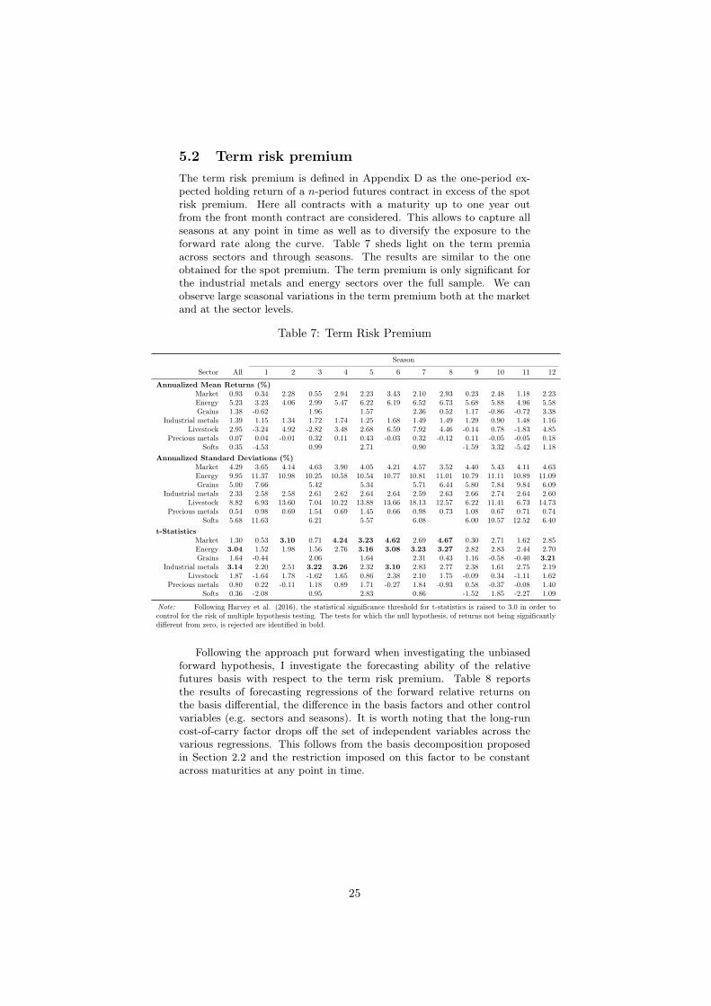
5.2 Term risk premium The term risk premium is defned in Appendix D as the one-period ex-pected holding return of a n-period futures contract in excess of the spot risk premium. Here all contracts with a maturity up to one year out from the front month contract are considered. This allows to capture all seasons at any point in time as well as to diversify the exposure to the forward rate along the curve. Table 7 sheds light on the term premia across sectors and through seasons. The results are similar to the one obtained for the spot premium. The term premium is only signifcant for the industrial metals and energy sectors over the full sample. We can observe large seasonal variations in the term premium both at the market and at the sector levels.

Table 7: Term Risk Premium

Season

Sector All 1 2 3 4 5 6 7 8 9 10 11 12

Annualized Mean Returns (%) Market 0.93 0.34 2.28 0.55 2.94 2.23 3.43 2.10 2.93 0.23 2.48 1.18 2.23 Energy 5.23 3.23 4.06 2.99 5.47 6.22 6.19 6.52 6.73 5.68 5.88 4.96 5.58 Grains 1.38 -0.62 1.96 1.57 2.36 0.52 1.17 -0.86 -0.72 3.38

Industrial metals 1.39 1.15 1.34 1.72 1.74 1.25 1.68 1.49 1.49 1.29 0.90 1.48 1.16 Livestock 2.95 -3.24 4.92 -2.82 3.48 2.68 6.59 7.92 4.46 -0.14 0.78 -1.83 4.85

Precious metals 0.07 0.04 -0.01 0.32 0.11 0.43 -0.03 0.32 -0.12 0.11 -0.05 -0.05 0.18 Softs 0.35 -4.53 0.99 2.71 0.90 -1.59 3.32 -5.42 1.18

Annualized Standard Deviations (%) Market 4.29 3.65 4.14 4.63 3.90 4.05 4.21 4.57 3.52 4.40 5.43 4.11 4.63 Energy 9.95 11.37 10.98 10.25 10.58 10.54 10.77 10.81 11.01 10.79 11.11 10.89 11.09 Grains 5.00 7.66 5.42 5.34 5.71 6.44 5.80 7.84 9.84 6.09

Industrial metals 2.33 2.58 2.58 2.61 2.62 2.64 2.64 2.59 2.63 2.66 2.74 2.64 2.60 Livestock 8.82 6.93 13.60 7.04 10.22 13.88 13.66 18.13 12.57 6.22 11.41 6.73 14.73

Precious metals 0.54 0.98 0.69 1.54 0.69 1.45 0.66 0.98 0.73 1.08 0.67 0.71 0.74 Softs 5.68 11.63 6.21 5.57 6.08 6.00 10.57 12.52 6.40

t-Statistics Market 1.30 0.53 3.10 0.71 4.24 3.23 4.62 2.69 4.67 0.30 2.71 1.62 2.85 Energy 3.04 1.52 1.98 1.56 2.76 3.16 3.08 3.23 3.27 2.82 2.83 2.44 2.70 Grains 1.64 -0.44 2.06 1.64 2.31 0.43 1.16 -0.58 -0.40 3.21

Industrial metals 3.14 2.20 2.51 3.22 3.26 2.32 3.10 2.83 2.77 2.38 1.61 2.75 2.19 Livestock 1.87 -1.64 1.78 -1.62 1.65 0.86 2.38 2.10 1.75 -0.09 0.34 -1.11 1.62

Precious metals 0.80 0.22 -0.11 1.18 0.89 1.71 -0.27 1.84 -0.93 0.58 -0.37 -0.08 1.40 Softs 0.36 -2.08 0.95 2.83 0.86 -1.52 1.85 -2.27 1.09


Following the approach put forward when investigating the unbiased forward hypothesis, I investigate the forecasting ability of the relative futures basis with respect to the term risk premium. Table 8 reports the results of forecasting regressions of the forward relative returns on the basis di˙erential, the di˙erence in the basis factors and other control variables (e.g. sectors and seasons). It is worth noting that the long-run cost-of-carry factor drops o˙ the set of independent variables across the various regressions. This follows from the basis decomposition proposed in Section 2.2 and the restriction imposed on this factor to be constant across maturities at any point in time.

25

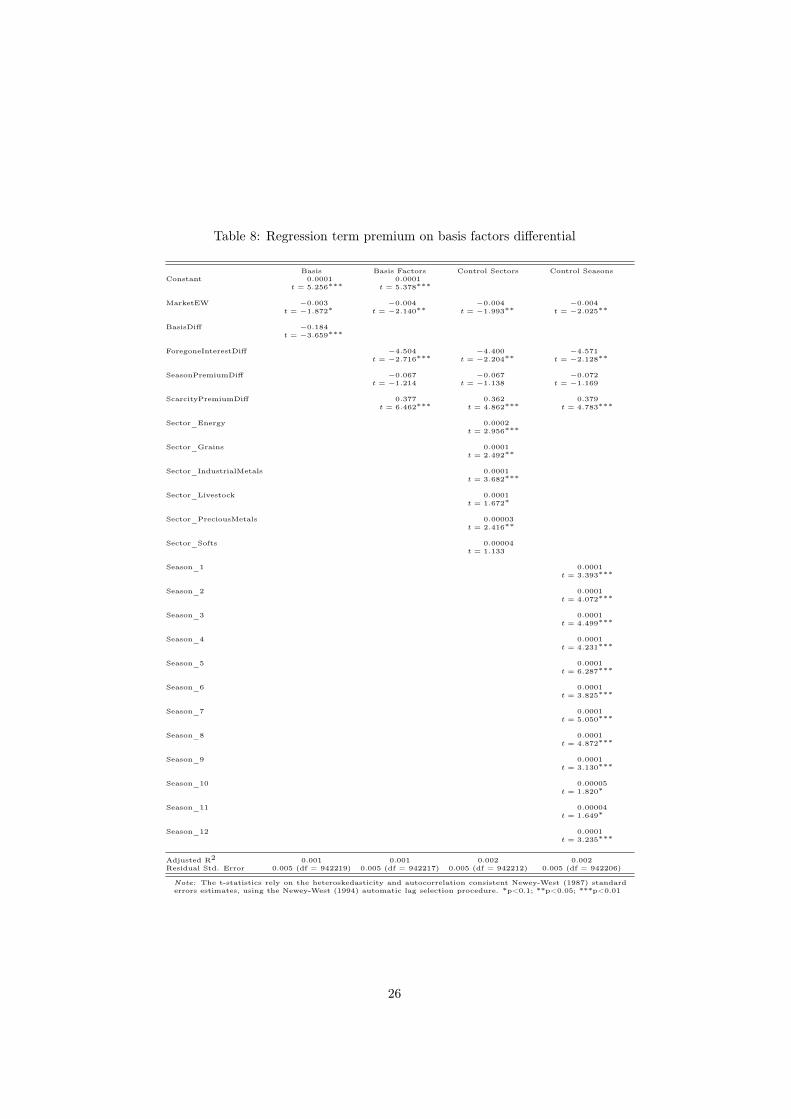
Table 8: Regression term premium on basis factors di˙erential

Constant Basis 0.0001

t = 5.256 ∗∗∗

Basis Factors 0.0001

t = 5.378 ∗∗∗

Control Sectors Control Seasons

MarketEW −0.003 t = −1.872 ∗

−0.004 t = −2.140 ∗∗

−0.004 t = −1.993 ∗∗

−0.004 t = −2.025 ∗∗

BasisDi˙ −0.184 t = −3.659 ∗∗∗

ForegoneInterestDi˙ −4.504 t = −2.716 ∗∗∗

−4.400 t = −2.204 ∗∗

−4.571 t = −2.128 ∗∗

SeasonPremiumDi˙ −0.067 t = −1.214

−0.067 t = −1.138

−0.072 t = −1.169

ScarcityPremiumDi˙ 0.377 t = 6.462 ∗∗∗

0.362 t = 4.862 ∗∗∗

0.379 t = 4.783 ∗∗∗

Sector_Energy 0.0002 t = 2.956 ∗∗∗

Sector_Grains 0.0001 t = 2.492 ∗∗

Sector_IndustrialMetals 0.0001 t = 3.682 ∗∗∗

Sector_Livestock 0.0001 t = 1.672 ∗

Sector_PreciousMetals 0.00003 t = 2.416 ∗∗

Sector_Softs 0.00004 t = 1.133

Season_1 0.0001 t = 3.393 ∗∗∗

Season_2 0.0001 t = 4.072 ∗∗∗

Season_3 0.0001 t = 4.499 ∗∗∗

Season_4 0.0001 t = 4.231 ∗∗∗

Season_5 0.0001 t = 6.287 ∗∗∗

Season_6 0.0001 t = 3.825 ∗∗∗

Season_7 0.0001 t = 5.050 ∗∗∗

Season_8 0.0001 t = 4.872 ∗∗∗

Season_9 0.0001 t = 3.130 ∗∗∗

Season_10 0.00005 t = 1.820 ∗

Season_11 0.00004 t = 1.649 ∗

Season_12 0.0001 t = 3.235 ∗∗∗

Adjusted R2

Residual Std. Error 0.001

0.005 (df = 942219) 0.001

0.005 (df = 942217) 0.002

0.005 (df = 942212) 0.002

0.005 (df = 942206)


26

The frst specifcation regresses the forward futures return relative to the front contract return against the market and the basis di˙erential. The basis di˙erential is highly signifcant and in line with expectations a high spread predicts negative relative returns. Although only signifcant at the 10% threshold it is worth highlighting the infuence of the market factor on the term premium whereby a rise in commodity markets leads to a negative term premium. To some extent this result is a refection of the correlation structure and relative risk along the futures curve, i.e. contracts further along the curve exhibit lower beta to spot changes. This e˙ect is consistent across the various regressions performed. Supportive evidence is provided by Table 9 which shows the panel full-sample corre-lation estimates of the frst twelve futures contract along the curve with the active contract as well as the volatilities of the contracts as we move along the curve (e.g. column 1 is the active front contract while column 3 refers to the third contract along the curve).

Table 9: Risk and correlation along the futures curve

1 2 3 4 5 6 7 8 9 10 11 12 Correlation 1.00 0.99 0.98 0.97 0.96 0.95 0.94 0.94 0.93 0.93 0.92 0.91

Volatility (%) 29.69 28.69 27.46 25.77 25.00 24.49 24.09 23.81 23.56 23.64 23.72 23.91

The second regression focuses on the various basis factors’ di˙erentials as explanatory variables of the forward relative returns. The frst factor di˙erential, the foregone interest one, is found to be signifcant at the 1% level. The sign of the coeÿcient is in line with expectations and the previous fndings on the spot risk premium. The second factor di˙erential, the seasonal premium one, is here as well not signifcant but the result is consistent with the fndings on the spot premium. This provides comfort in the interpretation put forward above. The last factor di˙erential, the scarcity premium one, is highly signifcant with a t-statistic well above 3. Here as well the results are consistent with earlier fndings.

The next two regressions introduce commodity sectors and seasons as control variables. As opposed to the results on the spot risk premium, here the control variables are often signifcant at the 5% level or lower. This hints at a large cross-sectional dispersion across sectors. With re-gards to seasons while these results suggest the term premium remains exposed to seasonal fuctuations it is worth mentioning this control vari-able only captures the season exposure of the far contract. The result for the scarcity premium are left unchanged suggesting those fndings are robust to the model specifcation.

5.3 Factor portfolios For all basis factors, Table 10 sheds light on the risk, return and t-statistic of quintiles portfolios implemented on the front contracts, together with those of the top-minus-bottom portfolio.

This table carries a few insightful results. First and foremost, the results confrm earlier literature fndings that the futures basis carries information about future returns. The t-statistics for the bottom quintile portfolio, which equally-weighs the commodity markets with the most negative basis (backwardated curves) is highly signifcant with a t-statistic of 3.26. It outperforms the top-minus-bottom portfolio which exhibits a

27

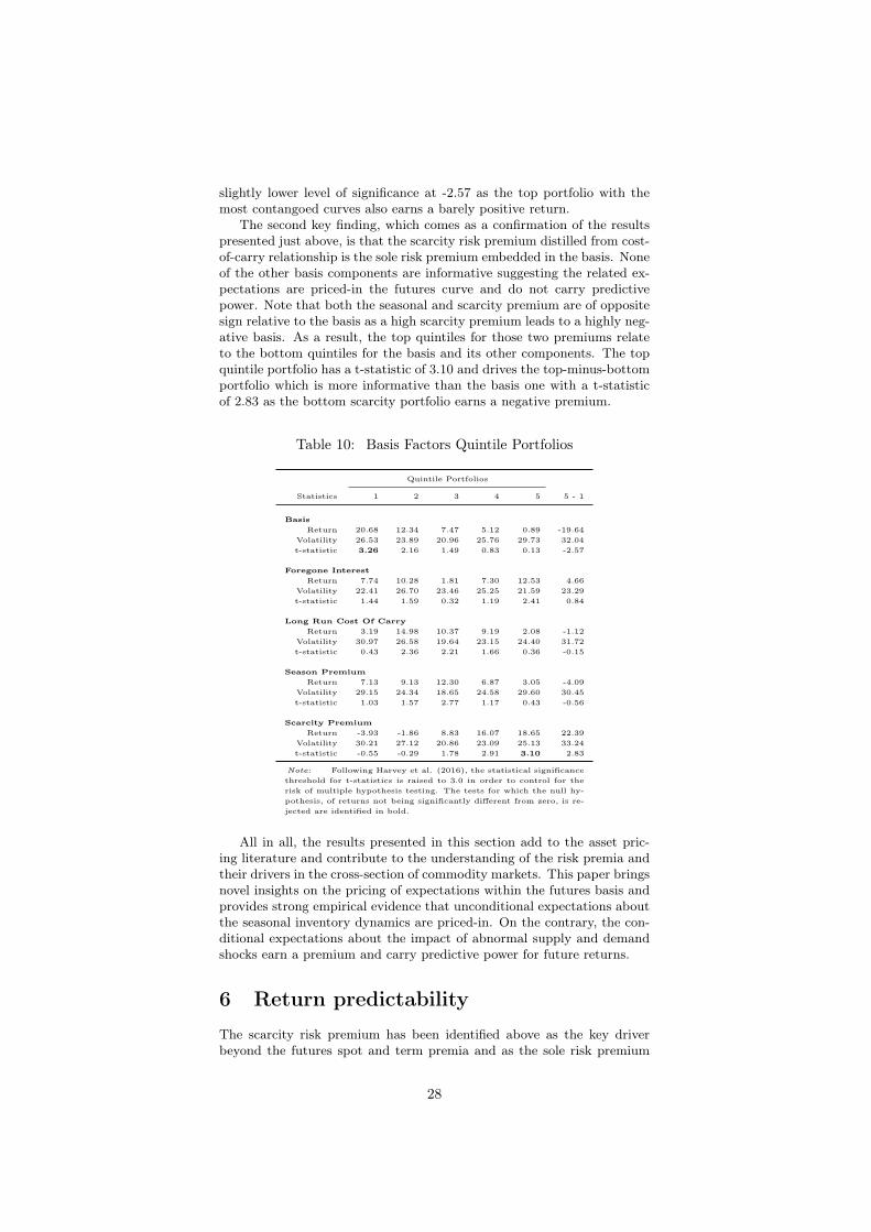
slightly lower level of signifcance at -2.57 as the top portfolio with the most contangoed curves also earns a barely positive return.

The second key fnding, which comes as a confrmation of the results presented just above, is that the scarcity risk premium distilled from cost-of-carry relationship is the sole risk premium embedded in the basis. None of the other basis components are informative suggesting the related ex-pectations are priced-in the futures curve and do not carry predictive power. Note that both the seasonal and scarcity premium are of opposite sign relative to the basis as a high scarcity premium leads to a highly neg-ative basis. As a result, the top quintiles for those two premiums relate to the bottom quintiles for the basis and its other components. The top quintile portfolio has a t-statistic of 3.10 and drives the top-minus-bottom portfolio which is more informative than the basis one with a t-statistic of 2.83 as the bottom scarcity portfolio earns a negative premium.

Table 10: Basis Factors Quintile Portfolios

Quintile Portfolios

Statistics 1 2 3 4 5 5 - 1

Basis

Return 20.68 12.34 7.47 5.12 0.89 -19.64 Volatility 26.53 23.89 20.96 25.76 29.73 32.04 t-statistic 3.26 2.16 1.49 0.83 0.13 -2.57

Foregone Interest

Return 7.74 10.28 1.81 7.30 12.53 4.66 Volatility 22.41 26.70 23.46 25.25 21.59 23.29 t-statistic 1.44 1.59 0.32 1.19 2.41 0.84

Long Run Cost Of Carry


Season Premium


Scarcity Premium

Return -3.93 -1.86 8.83 16.07 18.65 22.39 Volatility 30.21 27.12 20.86 23.09 25.13 33.24 t-statistic -0.55 -0.29 1.78 2.91 3.10 2.83

Note: Following Harvey et al. (2016), the statistical signifcance threshold for t-statistics is raised to 3.0 in order to control for the risk of multiple hypothesis testing. The tests for which the null hy-pothesis, of returns not being signifcantly di˙erent from zero, is re-jected are identifed in bold.

All in all, the results presented in this section add to the asset pric-ing literature and contribute to the understanding of the risk premia and their drivers in the cross-section of commodity markets. This paper brings novel insights on the pricing of expectations within the futures basis and provides strong empirical evidence that unconditional expectations about the seasonal inventory dynamics are priced-in. On the contrary, the con-ditional expectations about the impact of abnormal supply and demand shocks earn a premium and carry predictive power for future returns.

Return predictability

The scarcity risk premium has been identifed above as the key driver beyond the futures spot and term premia and as the sole risk premium

28

6

embedded in the futures basis but little is known on the origin of this return predictability. The eÿcient market hypothesis11 suggests that in the presence of shocks to supply and demand market participants adjust their expectations and incorporate instantaneously this new information in prices such that return predictability is precluded. Under such hypoth-esis the scarcity risk premium should refect the incorporation of new in-formation and the resulting expectations into the futures curve but should not be able to forecast forward returns.

At the same time commodity markets are characterized by the slow adjustment of demand and supply which leads to shock persistence. On the one hand, price inelastic demand originates from the absence of sub-stitutes in the short run. On the other hand, the supply of commodities is subject to the inelasticity of production in the short run driven by seasonal production cycles for perishable commodities and the long run e˙ects of investments and productivity increase on the total supply. Those two e˙ects combined result in a lengthy resolution of supply and demand imbalances.

Two potential competing but not mutually exclusive hypotheses could explain the observed return predictability. The frst one would be the presence of autocorrelation in unexpected net supply shocks such that selecting commodities on the basis of previous shocks would provide valu-able information about future expected returns. The second hypothesis would be that the slow di˙usion of information and/or market participants underreaction to new information lead to return predictability.12

6.1 Abnormal shocks serial correlation In order to asses the frst hypothesis of recurring shocks, I consider in Figure 5 the average autocorrelation coeÿcients up to one year across all combinations of market and season for the level and the change in the scarcity risk premium as it captures unexpected shocks to the net supply. While the dynamics of the level coeÿcients corroborates the persistence of shocks and the slow adjusment of fundamentals, the autocorrelation co-eÿcients for the changes in the scarcity risk premium cannot attest of the presence of a systematic recurrence of shocks through time. Indeed, the absence of large and signifcant autocorrelation coeÿcient for the change of the scarcity risk premium suggests unexpected shocks to supply and demand are not autocorrelated and I thus dismiss this frst hypothesis.

11See amongst others Malkiel and Fama (1970). 12Both behavioral phenomema have been widely documented in equity markets. See

amongst others the seminal paper of Jegadeesh and Titman (1993) for the underreaction of market participants. See amongst others Hong and Stein (1999) and Hong et al. (2000) for the slow di˙usion of information. Dissociating those two potential sources of return predictability is beyond the scope of this paper.

29

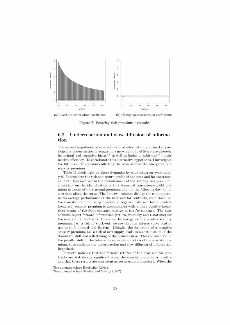
0 50 100 150 200 250

0.0

0.2

0.4

0.6

0.8

1.0

Lag (Days)

Aut

ocor

rela

tion

Coe

ffici

ent

0 50 100 150 200 250

0.0

0.2

0.4

0.6

0.8

1.0

Lag (Days)

Aut

ocor

rela

tion

Coe

ffici

ent

(a) Level autocorrelation coeÿcients (b) Change autocorrelation coeÿcients

Figure 5: Scarcity risk premium dynamics

6.2 Underreaction and slow di˙usion of informa-tion The second hypothesis of slow di˙usion of information and market par-ticipants underreaction leverages on a growing body of literature whereby behavioral and cognitive biases13 as well as limits to arbitrage14 impair market eÿciency. To corroborate this alternative hypothesis, I investigate the futures curve dynamics a˙ecting the basis around the emergence of a scarcity premium.

Table 11 sheds light on those dynamics by conducting an event anal-ysis. It considers the risk and return profle of the near and far contracts, i.e. both legs involved in the measurement of the scarcity risk premium, coincident on the identifcation of this abnormal convenience yield pre-mium in excess of the seasonal premium, and, on the following day, for all contracts along the curve. The frst two columns display the contempora-neous average performance of the near and far contracts, conditional on the scarcity premium being positive or negative. We see that a positive (negative) scarcity premium is accompanied with a more positive (nega-tive) return of the front contract relative to the far contract. The next columns report forward information (return, volatility and t-statistic) for the near and far contracts. Following the emergence of a positive scarcity premium, i.e. a risk of stock-out, we see that the futures curve contin-ues to shift upward and fattens. Likewise the formation of a negative scarcity premium, i.e. a risk of oversupply, leads to a continuation of the downward shift and a fattening of the futures curve. This continuation in the parallel shift of the futures curve, in the direction of the scarcity pre-mium, thus confrms the underreaction and slow di˙usion of information hypothesis.

It worth noticing that the forward returns of the near and far con-tracts are statistically signifcant when the scarcity premium is positive and that those results are consistent across seasons and sectors. When the

13See amongst others Hirshleifer (2001). 14See amongst others Shleifer and Vishny (1997).

30

scarcity premium is negative the forward returns are not statistically sig-nifcant and results are not consistent through sectors or seasons. These results provides evidence that market participants underreact to the risk of scarcity and suggest the scarcity premium is truly a compensation for the risk of stock-out.

Table 11: Curve Dynamics

Information Contemporaneous Forward

Contract Near Far Near Far

Sector/Season Return Return Return Volatility t-statistic Return Volatility t-statistic

Positive scarcity premium Average 17.50 14.29 5.92 12.22 2.89 7.98 12.05 3.95

Energy 17.96 14.71 7.33 22.24 1.85 9.45 21.47 2.47 Grains 12.02 8.20 4.05 18.59 1.29 7.13 18.29 2.30

Industrial metals 23.25 19.60 10.74 22.44 2.22 12.62 22.08 2.65 Livestock 10.99 4.95 3.10 12.47 1.37 6.49 12.05 2.96

Precious metals 3.20 1.68 0.23 23.73 0.05 1.71 23.69 0.39 Softs 15.34 10.76 -0.05 18.06 -0.01 2.58 17.76 0.86

1 18.05 15.14 5.88 14.41 2.38 8.02 14.24 3.28 2 19.42 16.65 7.08 14.27 2.88 8.72 14.05 3.60 3 18.43 15.67 8.61 13.93 3.63 10.42 13.79 4.44 4 21.88 18.55 6.16 13.82 2.58 8.72 13.52 3.73 5 19.47 16.22 7.19 13.91 3.01 9.68 13.70 4.12 6 18.19 14.07 4.86 13.74 2.05 7.65 13.58 3.27 7 16.82 13.96 7.15 14.31 2.92 9.11 14.16 3.76 8 20.29 16.54 6.17 13.76 2.60 8.69 13.46 3.74 9 16.62 12.95 6.22 13.39 2.71 8.41 13.20 3.71

10 16.28 13.19 3.77 13.35 1.65 5.21 13.13 2.32 11 14.67 12.44 3.53 13.13 1.57 5.27 12.96 2.37 12 12.59 10.60 3.60 13.10 1.61 5.22 13.01 2.36

Negative scarcity premium Average -10.18 -7.54 -0.72 12.53 -0.34 -2.13 12.35 -1.03

Energy -1.53 1.73 8.07 25.19 1.79 6.18 24.31 1.42 Grains -6.36 -3.03 -0.93 18.25 -0.30 -2.88 17.94 -0.95

Industrial metals -3.34 -1.62 1.81 21.82 0.42 0.92 21.64 0.21 Livestock -2.73 3.54 4.28 13.06 1.79 0.67 12.33 0.30

Precious metals -4.61 -2.94 -0.09 21.28 -0.02 -1.78 21.22 -0.50 Softs -13.88 -11.15 -1.31 15.58 -0.50 -2.78 15.23 -1.09

1 -13.35 -10.75 -2.63 13.09 -1.16 -4.10 12.88 -1.84 2 -11.78 -9.54 -2.64 13.41 -1.15 -3.57 13.23 -1.58 3 -8.98 -6.74 -2.29 13.46 -1.00 -3.29 13.30 -1.46 4 -11.24 -8.27 0.74 13.14 0.33 -0.83 12.93 -0.37 5 -9.25 -6.24 0.81 13.55 0.35 -0.73 13.39 -0.32 6 -9.91 -6.68 -0.07 14.23 -0.03 -2.07 14.13 -0.86 7 -10.36 -7.85 -2.15 14.10 -0.88 -3.52 13.97 -1.46 8 -11.81 -8.89 0.49 13.95 0.21 -1.48 13.67 -0.63 9 -9.69 -6.78 -0.64 13.89 -0.27 -2.48 13.68 -1.06

10 -10.82 -8.60 1.18 14.52 0.48 -0.25 14.37 -0.10 11 -9.01 -6.83 0.96 14.10 0.40 -0.27 13.88 -0.12 12 -10.01 -7.89 -1.72 13.98 -0.72 -2.80 13.84 -1.19


Another interesting result relates to the curve twisting, i.e. fattening or steepening, originating from a more pronounced underreaction in the far contract. This implies that the underestimation of the probability of

31

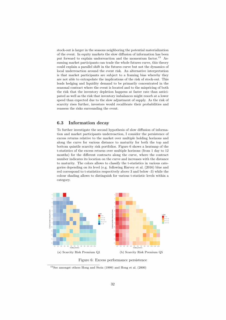
stock-out is larger in the seasons neighboring the potential materialization of the event. In equity markets the slow di˙usion of information has been put forward to explain underreaction and the momentum factor.15 As-suming market participants can trade the whole futures curve, this theory could explain a parallel shift in the futures curve but not the dynamics of local underreaction around the event risk. An alternative interpretation is that market participants are subject to a framing bias whereby they are not able to extrapolate the implications of the risk of stock-out. This leads hedging and liquidity demand to be primarily concentrated in the seasonal contract where the event is located and to the mispricing of both the risk that the inventory depletion happens at faster rate than antici-pated as well as the risk that inventory imbalances might resorb at a lower speed than expected due to the slow adjustment of supply. As the risk of scarcity rises further, investors would recalibrate their probabilities and reassess the risks surrounding the event.

6.3 Information decay To further investigate the second hypothesis of slow di˙usion of informa-tion and market participants underreaction, I consider the persistence of excess returns relative to the market over multiple holding horizons and along the curve for various distance to maturity for both the top and bottom quintile scarcity risk portfolios. Figure 6 shows a heatmap of the t-statistics of the excess returns over multiple horizons (from 1 day to 12 months) for the di˙erent contracts along the curve, where the contract number indicates its location on the curve and increases with the distance to maturity. The colors allows to classify the t-statistics in various cate-gories depending on its level (e.g. following Harvey et al. (2016) blue and red correspond to t-statistics respectively above 3 and below -3) while the colour shading allows to distinguish for various t-statistic levels within a category.

14

13

12

11

10

9

8

7

6

5

4

3

2

1D 1M 2M 3M 4M 5M 6M 7M 8M 9M 10M 11M 12MHolding Horizon

Con

trac

t num

ber

alon

g th

e C

urve

t−Stat

t >= 3

0 <= t < 2

−2 < t < 0

−3 < t <= −2

t <= −3

14

13

12

11

10

9

8

7

6

5

4

3

2

1D 1M 2M 3M 4M 5M 6M 7M 8M 9M 10M 11M 12MHolding Horizon

Con

trac

t num

ber

alon

g th

e C

urve

t−Stat

t >= 3

2 <= t < 3

0 <= t < 2

−2 < t < 0

(a) Scarcity Risk Premium Q1 (b) Scarcity Risk Premium Q5

Figure 6: Excess performance persistence

15See amongst others Hong and Stein (1999) and Hong et al. (2000)

32

Beyond allowing to detect the presence of excess returns’ persistence, associated with forecasting power, this representation carries valuable in-formation. First, by conditioning on the quintile number it allows to distinguish the direction of the excess return predictability between high and low scarcity risk. Second, by evaluating multiple holding horizons, this analysis allows to assess the decay in the excess return over time and thus to defne the return predictability horizon. Third, by considering the whole futures curve, we can identify whether the excess returns are uniformly distributed along the curve or whether they are concentrated in a specifc location (e.g. the front end) of the curve.

We see from Figure 6a that an unexpected risk of over-supply, i.e. a negative scarcity risk premium, leads to negative highly signifcant excess returns over the market for a holding horizon up to 3 months. This pattern is mostly observable in the front end of the curve, for contract with a time to maturity up to 9 months. Figure 6b shows that unexpected risks of scarcity, i.e. a positive premium is associated with highly signifcant positive excess returns over the market across the whole curve for a holding horizon up to 3 months.

In both fgures we observe that the excess returns are transient and most signifcant right after the unexpected shocks, suggesting the informa-tion is largely incorporated by market participants without delay. Their diminishing signifcance with the length of the holding horizon indicates that the information is progressively di˙used throughout the market up until it is fully incorporated in futures prices. More importantly, their short persistence through time, i.e. a high alpha decay, seems inconsis-tent with the expected timelines of a fundamentally driven resolution of supply and demand imbalances.

The results presented in this section bring convincing evidence that the scarcity risk premium is a compensation for the risk of stock-out. It fnds its origin in the slow di˙usion of information and underreaction to abnormal changes in inventories, above and beyond seasonal dynamics. The underreaction is broad based along the curve and is more pronounced in the far contracts, leading to curve twist and suggesting market partici-pants also underreact to the risk that the inventory depletion happens at faster rate than anticipated as well as the risk that inventory imbalances might resorb at a lower speed than expected due to the slow adjustment of supply. While most of the information is incorporated shortly after the materialization of the risk of stock-out, the return predictability horizon is about 3 months which is long enough to support the underreaction and slow di˙usion of information hypothesis and too short to be associated with a fundamental resolution of abnormal supply and demand imbal-ances.

Conclusion

The cost-of-carry relationship is the corner stone of the theory of stor-age. It assumes the di˙erence between the futures and spot prices, i.e. the futures basis, can be explained by the interest foregone when buying commodities in the physical market, the associated storage costs and a convenience yield. The latter is defned as a beneft that accrues to the

33

commodity holder resulting from the potential productive value of his in-ventory. This value of physical ownership refects market expectations about the future availability of a commodity.

A vast literature provides evidence that the futures basis is informa-tive about futures risk premia. This paper sheds light on the origin of this return predictability by disentangling various expectations embedded in the basis. As production and demand seasonality can have a large infuence on the future state of inventories, a convenience yield decompo-sition is proposed to dissociate known seasonal supply and demand imbal-ances from abnormal shocks above and beyond those transitory dynamics. Agents form expectations about the impact of inventories’ seasonality on the basis (henceforth the seasonality risk premium) and adjust their con-ditional expectations as new information arrives. Changes in expectations resulting from unanticipated supply and demand shocks (henceforth the scarcity risk premium) are associated with the incremental risk of scarcity and capture the non-linearities in the futures basis.

The contribution of this paper to the asset pricing literature is three-fold. First, it brings novel insights on the fundamental relationship be-tween the futures basis and inventory dynamics. While the literature has documented the relationship between the basis and the level of inventories, as well as the presence of seasonality in both the basis and the inventories, the question of how various inventory dynamics are priced in the cross-section of commodity markets remains an open research topic. This paper investigates whether the predictable seasonality in the convenience yield is related to known seasonal fuctuations in inventories, and whether the residual, or seasonally-adjusted, convenience yield is associated with unex-pected supply and demand shocks. It provides strong empirical evidence that the convenience yield embeds expectations about those two di˙erent inventory dynamics. On one hand, the seasonal risk premium captures expectations about the inventory seasonalities. On the other hand, the scarcity risk premium refects the excess supply and demand imbalances over the expected seasonal fuctuations.

Second, this paper contributes to the understanding of the risk premia in the cross-section of commodity markets by investigating the pricing of expectations within the futures basis. It provides strong empirical evidence that the seasonality risk premium is priced-in as unconditional expectations about the seasonal inventory dynamics carry no predictive power. On the contrary, the conditional expectations about the impact of abnormal supply and demand shocks earn a premium and carry predictive power for future returns. In fne, the scarcity risk premium carries all the predictive power embedded in the futures basis. Other basis components, i.e. the foregone interest and the net cost of storage, have no information content. Those fndings are robust to the introduction of commodity sectors and seasons as control variables.

The third contribution of this paper is to show that the scarcity risk premium is a compensation for the unexpected increase in the risk of stock-out and that the associated return predictability fnds its origin in the slow di˙usion of information and underreaction to abnormal changes in inventories, above and beyond seasonal dynamics. It presents strong evidence of underreaction along the futures curve following a marginal change in the risk of stock-out. The underreaction is broad based along the curve but more pronounced in the far contracts, leading to futures curve twists. These results suggest that market participants also under-

34

react to the risk that the inventory depletion happens at faster rate than anticipated, as well as the risk that inventory imbalances might resorb at a lower speed than expected due to the slow adjustment of supply. Despite the slow di˙usion of information and the unexpected nature of the supply and demand shocks, information decays fast and the return predictability is transient. The diminishing statistical signifcance of excess returns with the length of the holding horizon indicates that the information is pro-gressively di˙used throughout the market up until it is fully incorporated in futures prices. The scarcity risk premium has signifcant predictive power up to a 3 months horizon, which is too short to be associated with a fundamental resolution of abnormal supply and demand imbalances.

As the probability of stock-out increases, the net hedging demand rises. On one hand, commodity consumers need to hedge out the scarcity risk by buying spot and storing the commodity or by taking long futures positions with delivery at the time of likely scarcity. On the other hand, producers would beneft from unwinding their hedges or taking outright long commodity exposures when inventory levels are low and eroding.16

At the same time, other informed market participants, e.g. speculators, know about the predictive power embedded in the basis. The question of who might be a willing counterparty to the hedging and speculative demand in the presence of scarcity risk thus deserves further research.

Another avenue of research relates to the pricing of expectations along the futures curve. On one hand, this paper provides empirical evidence that the seasonality risk premium is priced-in and carries no predictive power. On the other hand, Keloharju et al. (2016) fnd strong evidence of the presence of returns seasonality in U.S. and international equities as well as in commodities. Although the authors fnd that for the later the di˙erence between the high and low seasonal portfolios is only marginally statistically signifcant but economically important, the questions of what the drivers of the return seasonality factor are and how it relates to the seasonality risk premium defned in this paper warrant additional research.

16Hirshleifer (1991) refutes the general pre-conception of a short hedging pressure resulting from producers simply willing to hedge their bottom line volatility. He argues that when demand shocks are arising from changes in aggregate wealth, the optimal hedging policy of producers with non-stochastic output might be to remain unhedged or even to take a long hedge position.

35

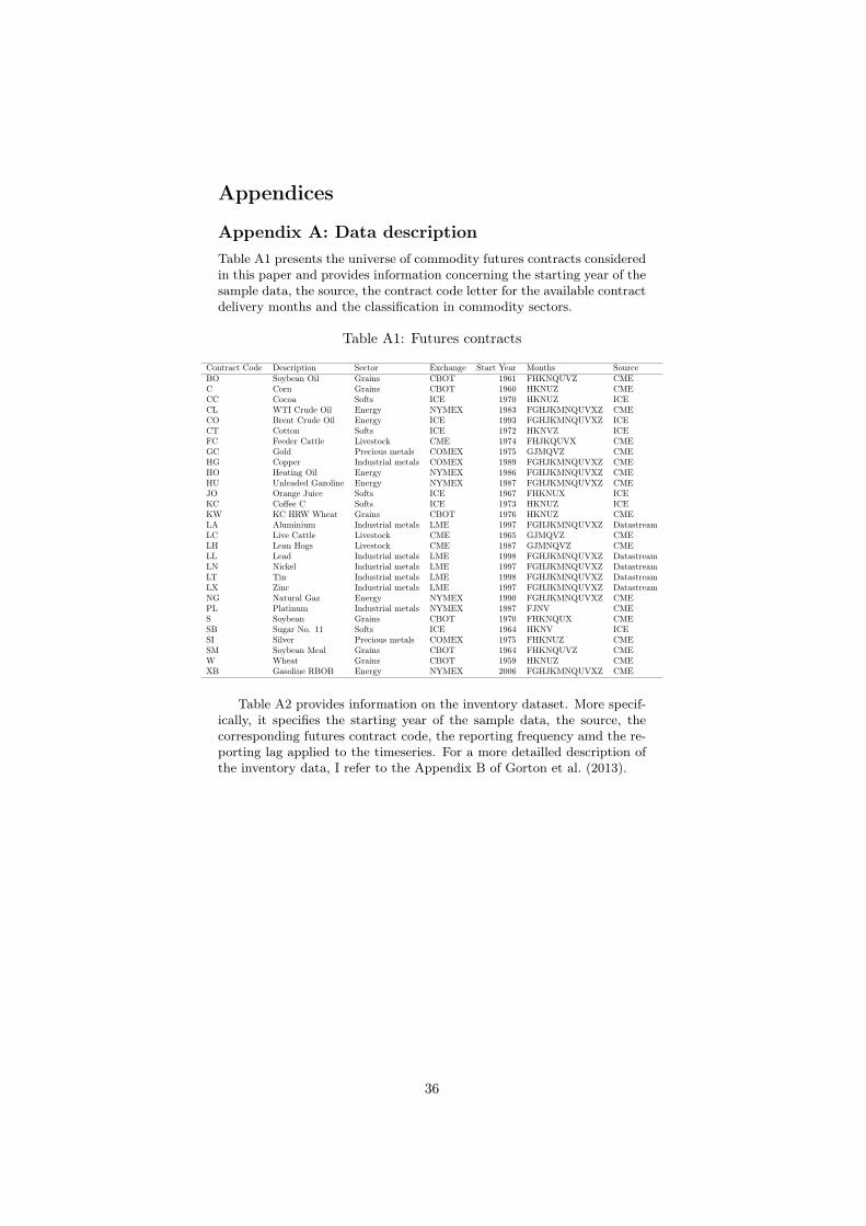
Appendices

Appendix A: Data description Table A1 presents the universe of commodity futures contracts considered in this paper and provides information concerning the starting year of the sample data, the source, the contract code letter for the available contract delivery months and the classifcation in commodity sectors.

Table A1: Futures contracts

Contract Code Description Sector Exchange Start Year Months Source BO Soybean Oil Grains CBOT 1961 FHKNQUVZ CME C Corn Grains CBOT 1960 HKNUZ CME CC Cocoa Softs ICE 1970 HKNUZ ICE CL WTI Crude Oil Energy NYMEX 1983 FGHJKMNQUVXZ CME CO Brent Crude Oil Energy ICE 1993 FGHJKMNQUVXZ ICE CT Cotton Softs ICE 1972 HKNVZ ICE FC Feeder Cattle Livestock CME 1974 FHJKQUVX CME GC Gold Precious metals COMEX 1975 GJMQVZ CME HG Copper Industrial metals COMEX 1989 FGHJKMNQUVXZ CME HO Heating Oil Energy NYMEX 1986 FGHJKMNQUVXZ CME HU Unleaded Gazoline Energy NYMEX 1987 FGHJKMNQUVXZ CME JO Orange Juice Softs ICE 1967 FHKNUX ICE KC Co˙ee C Softs ICE 1973 HKNUZ ICE KW KC HRW Wheat Grains CBOT 1976 HKNUZ CME LA Aluminium Industrial metals LME 1997 FGHJKMNQUVXZ Datastream LC Live Cattle Livestock CME 1965 GJMQVZ CME LH Lean Hogs Livestock CME 1987 GJMNQVZ CME LL Lead Industrial metals LME 1998 FGHJKMNQUVXZ Datastream LN Nickel Industrial metals LME 1997 FGHJKMNQUVXZ Datastream LT Tin Industrial metals LME 1998 FGHJKMNQUVXZ Datastream LX Zinc Industrial metals LME 1997 FGHJKMNQUVXZ Datastream NG Natural Gaz Energy NYMEX 1990 FGHJKMNQUVXZ CME PL Platinum Industrial metals NYMEX 1987 FJNV CME S Soybean Grains CBOT 1970 FHKNQUX CME SB Sugar No. 11 Softs ICE 1964 HKNV ICE SI Silver Precious metals COMEX 1975 FHKNUZ CME SM Soybean Meal Grains CBOT 1964 FHKNQUVZ CME W Wheat Grains CBOT 1959 HKNUZ CME XB Gasoline RBOB Energy NYMEX 2006 FGHJKMNQUVXZ CME

Table A2 provides information on the inventory dataset. More specif-ically, it specifes the starting year of the sample data, the source, the corresponding futures contract code, the reporting frequency amd the re-porting lag applied to the timeseries. For a more detailled description of the inventory data, I refer to the Appendix B of Gorton et al. (2013).

36

Table A2: Commodity inventories

Contract Code Description Source Frequency Start Year Lag BO Soybean Oil USDA Monthly 1964 1 Month C Corn USDA Monthly 1960 1 Month CC Cocoa ICE Daily 2012 1 Day CL WTI Crude Oil DOE Weekly 1982 1 Week CO Brent Crude Oil CT Cotton ICE Daily 2002 1 Day FC Feeder Cattle USDA Monthly 1994 1 Month GC Gold COMEX Daily 1992 1 Day HG Copper COMEX Daily 1992 1 Day HO Heating Oil DOE Weekly 1993 1 Week HU Unleaded Gazoline DOE Weekly 2004 1 Week JO Orange Juice USDA Monthly 1964 1 Month KC Co˙ee C ICE Daily 2010 1 Day KW KC HRW Wheat CBOT Weekly 2008 1 Week LA Aluminium LME Daily 1978 1 Day LC Live Cattle USDA Monthly 1917 1 Month LH Lean Hogs USDA Monthly 1917 1 Month LL Lead LME Daily 1970 1 Day LN Nickel LME Daily 1979 1 Day LT Tin LME Daily 1970 1 Day LX Zinc LME Daily 1970 1 Day NG Natural Gaz DOE Monthly 1973 1 Month PL Platinum NYMEX Daily 1995 1 Day S Soybean USDA Monthly 1964 1 Month SB Sugar No. 11 USDA Monthly 1996 1 Month SI Silver COMEX Daily 1992 1 Day SM Soybean Meal USDA Monthly 1964 1 Month W Wheat USDA Monthly 1960 1 Month XB Gasoline RBOB DOE Weekly 2004 1 Week

37

Appendix B: Estimation of the seasonal premium Tables B1, B2, B3 and B4 show the full-sample estimates of the seasonal premium over the long-run cost-of-carry per commodity. The estimation has been carried out by means of robust regression using a panel approach along the futures curve, i.e. considering all available contracts at any point in time, using seasonal dummies. The results are reported using Newey-West standard errors, i.e. heteroskedasticity and autocorrelation consistent estimate of the covariance matrix of the coeÿcient estimates.

38

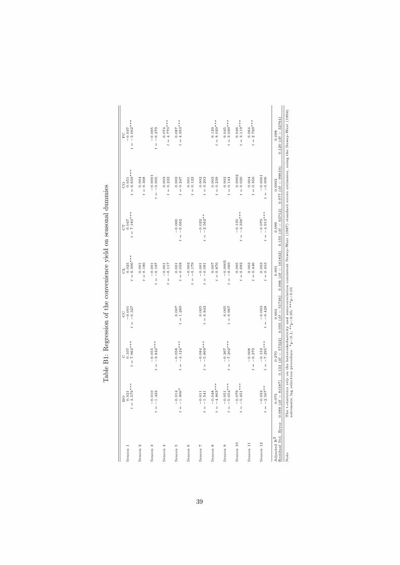
39

Tab

le B

1: R

egression of the con

venience yield on season

al dum

mies

BO

CCC

CL

CT

CO

FC

Season 1

0.021

0.107

−0.001

0.025

0.047

0.051

−0.037

t

=3.579∗∗∗

t

=7.964∗∗∗

t

= −0.327

t

=6.306∗∗∗

t

=7.183∗∗∗

t

=6.659∗∗∗

t

= −3.002∗∗∗

Season 2

0.001

0.004

t

=0.186

t

=0.368

Season 3

−0.010

−0.055

−0.001

−0.0001

−0.005

t

= −1.423

t

= −3.842∗∗∗

t

= −0.197

t

= −0.005

t

= −0.279

Season 4

−0.001

0.003

0.074

t

= −0.117

t

=0.232

t

=4.770∗∗∗

Season 5

−0.014

−0.058

0.007

0.001

−0.006

0.003

0.087

t

= −1.900∗

t

= −4.124∗∗∗

t

=1.260

t

=0.058

t

= −0.662

t

=0.247

t

=4.953∗∗∗

Season 6

−0.002

0.001

t

= −0.179

t

=0.122

Season 7

−0.011

−0.084

0.005

−0.001

−0.022

0.002

t

= −1.541

t

= −5.869∗∗∗

t

=0.842

t

= −0.091

t

= −2.562∗∗

t

=0.203

Season 8

−0.048

0.007

0.003

0.129

t

= −4.863∗∗∗

t

=0.876

t

=0.239

t

=9.029∗∗∗

Season 9

−0.051

−0.267

0.005

−0.0005

0.002

0.045

t

= −5.054∗∗∗

t

= −7.202∗∗∗

t

=0.967

t

= −0.069

t

=0.144

t

=3.039∗∗∗

Season 10

−0.079

0.005

−0.135

0.0002

0.046

t

= −5.051∗∗∗

t

=0.692

t

= −4.338∗∗∗

t

=0.020

t

=3.119∗∗∗

Season 11

−0.008

0.003

0.004

0.064

t

= −0.379

t

=0.446

t

=0.350

t

=2.769∗∗∗

Season 12

−0.024

−0.153

−0.003

0.003

−0.079

−0.0001

t

= −2.567∗∗

t

= −7.295∗∗∗

t

= −0.428

t

=0.453

t

= −4.913∗∗∗

t

= −0.006

Adjusted R2

0.075

0.270

0.004

0.001

0.099

0.0003

0.098

Residual Std. Error

0.089 (df = 81587)

0.133 (df = 57322)

0.055 (df = 51736)

0.096 (df = 161832)

0.155 (df = 63712)

0.077 (df = 99610)

0.120 (df = 32764)

Note

The t-statistics rely on the heteroskedasticity and autocorrelation consistent New

ey-W

est (1987) standard errors estim

ates, using the New

ey-W

est (1994)

automatic lag selection procedure. *p<0.1; **p<0.05; ***p<0.01

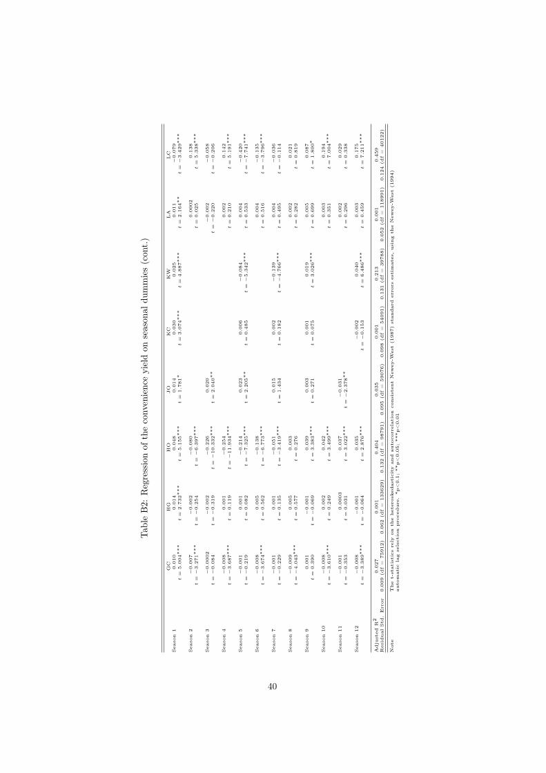
40

Tab

le B

2: R



al dum

mies (con

t.)

GC

HG

HO

JO

KC

KW

LA

LC

Season 1

0.010

0.014

0.048

0.014

0.030

0.025

0.011

−0.079

t

=5.004∗∗∗

t

=2.732∗∗∗

t

=5.155∗∗∗

t

=1.781∗

t

=3.074∗∗∗

t

=4.887∗∗∗

t

=2.164∗∗

t

= −3.429∗∗∗

Season 2

−0.007

−0.002

−0.080

0.0002

0.138

t

= −3.271∗∗∗

t

= −0.254

t

= −6.397∗∗∗

t

=0.025

t

=5.338∗∗∗

Season 3

−0.0002

−0.002

−0.226

0.020

−0.002

−0.058

t

= −0.084

t

= −0.319

t

= −10.332∗∗∗

t

=2.040∗∗

t

= −0.220

t

= −0.206

Season 4

−0.008

0.001

−0.254

0.002

0.142

t

= −3.687∗∗∗

t

=0.119

t

= −11.934∗∗∗

t

=0.210

t

=5.191∗∗∗

Season 5

−0.001

0.001

−0.214

0.023

0.006

−0.084

0.004

−0.420

t

= −0.219

t

=0.082

t

= −7.325∗∗∗

t

=2.205∗∗

t

=0.485

t

= −5.342∗∗∗

t

=0.533

t

= −7.741∗∗∗

Season 6

−0.008

0.005

−0.138

0.004

−0.135

t

= −3.674∗∗∗

t

=0.562

t

= −6.773∗∗∗

t

=0.516

t

= −3.796∗∗∗

Season 7

−0.001

0.001

−0.051

0.015

0.002

−0.139

0.004

−0.036

t

= −0.229

t

=0.135

t

= −3.419∗∗∗

t

=1.434

t

=0.182

t

= −4.766∗∗∗

t

=0.495

t

= −0.114

Season 8

−0.009

0.005

0.003

0.002

0.021

t

= −4.043∗∗∗

t

=0.577

t

=0.276

t

=0.282

t

=0.819

Season 9

0.001

−0.001

0.039

0.003

0.001

0.019

0.005

0.087

t

=0.390

t

= −0.069

t

=3.383∗∗∗

t

=0.271

t

=0.075

t

=3.026∗∗∗

t

=0.699

t

=1.800∗

Season 10

−0.008

0.002

0.042

0.003

0.194

t

= −3.610∗∗∗

t

=0.249

t

=3.499∗∗∗

t

=0.351

t

=7.004∗∗∗

Season 11

−0.001

0.0003

0.037

−0.031

0.002

0.029

t

= −0.353

t

=0.031

t

=3.022∗∗∗

t

= −2.378∗∗

t

=0.296

t

=0.338

Season 12

−0.008

−0.001

0.035

−0.002

0.040

0.003

0.175

t

= −3.389∗∗∗

t

= −0.064

t

=2.876∗∗∗

t

= −0.153

t

=6.486∗∗∗

t

=0.459

t

=7.211∗∗∗

Adjusted R2

0.027

0.001

0.404

0.035

0.001

0.213

0.001

0.459

Residual Std. Error

0.009 (df = 75912)

0.062 (df = 133629)

0.132 (df = 98791)

0.095 (df = 59076)

0.098 (df = 54091)

0.131 (df = 39788)

0.052 (df = 118991)

0.124 (df = 40122)

Note


ey-W


ates, using the New

ey-W

est (1994)


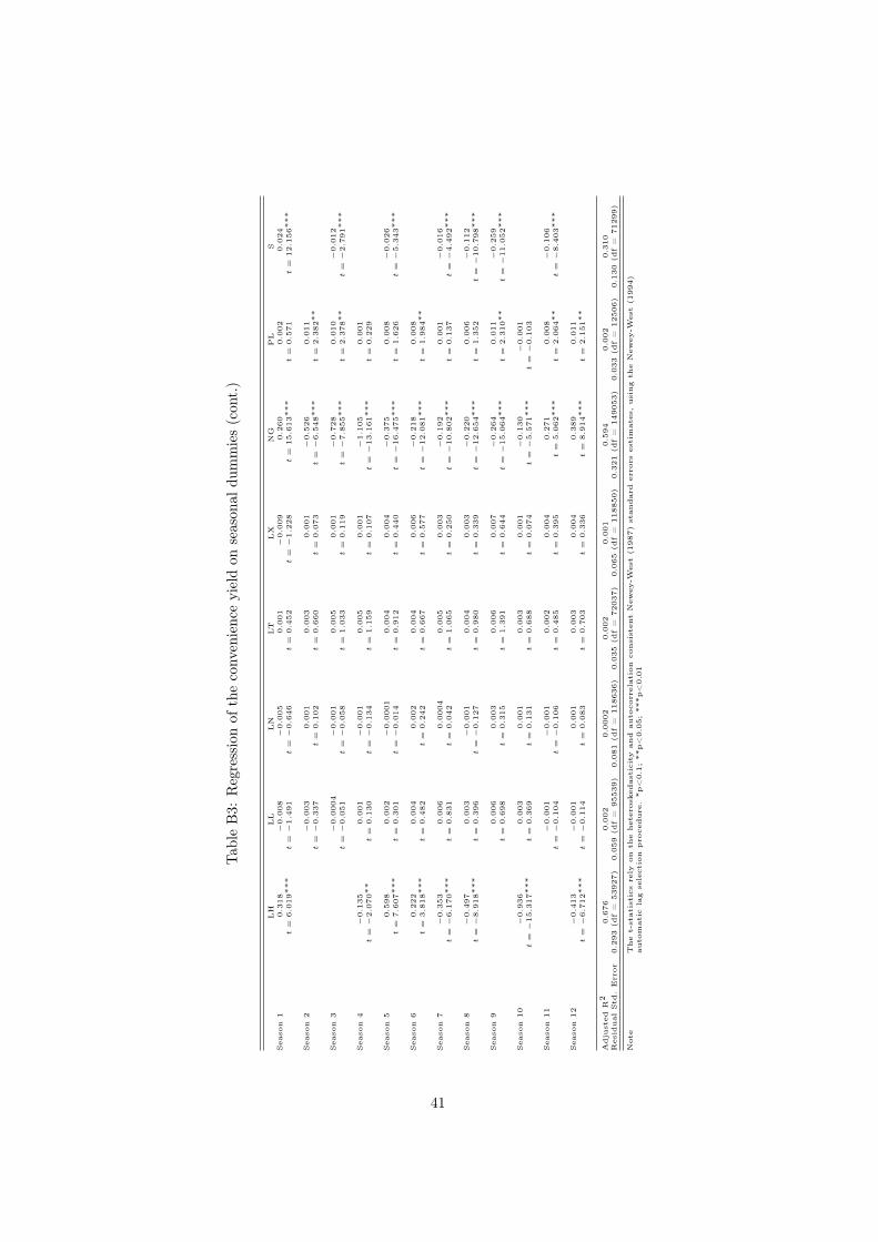
41

Tab

le B

3: R



al dum

mies (con

t.)

LH

LL

LN

LT

LX

NG

PL

S

Season 1

0.318

−0.008

−0.005

0.001

−0.009

0.260

0.002

0.024

t

=6.019∗∗∗

t

= −1.491

t

= −0.646

t

=0.452

t

= −1.228

t

= 15.613∗∗∗

t

=0.571

t

= 12.156∗∗∗

Season 2

−0.003

0.001

0.003

0.001

−0.526

0.011

t

= −0.337

t

=0.102

t

=0.660

t

=0.073

t

= −6.548∗∗∗

t

=2.382∗∗

Season 3

−0.0004

−0.001

0.005

0.001

−0.728

0.010

−0.012

t

= −0.051

t

= −0.058

t

=1.033

t

=0.119

t

= −7.855∗∗∗

t

=2.378∗∗

t

= −2.791∗∗∗

Season 4

−0.135

0.001

−0.001

0.005

0.001

−1.105

0.001

t

= −2.070∗∗

t

=0.130

t

= −0.134

t

=1.159

t

=0.107

t

= −13.161∗∗∗

t

=0.229

Season 5

0.598

0.002

−0.0001

0.004

0.004

−0.375

0.008

−0.026

t

=7.607∗∗∗

t

=0.301

t

= −0.014

t

=0.912

t

=0.440

t

= −16.475∗∗∗

t

=1.626

t

= −5.343∗∗∗

Season 6

0.222

0.004

0.002

0.004

0.006

−0.218

0.008

t

=3.818∗∗∗

t

=0.482

t

=0.242

t

=0.667

t

=0.577

t

= −12.081∗∗∗

t

=1.984∗∗

Season 7

−0.353

0.006

0.0004

0.005

0.003

−0.192

0.001

−0.016

t

= −6.170∗∗∗

t

=0.831

t

=0.042

t

=1.065

t

=0.250

t

= −10.802∗∗∗

t

=0.137

t

= −4.492∗∗∗

Season 8

−0.497

0.003

−0.001

0.004

0.003

−0.220

0.006

−0.112

t

= −8.918∗∗∗

t

=0.396

t

= −0.127

t

=0.980

t

=0.339

t

= −12.654∗∗∗

t

=1.352

t

= −10.798∗∗∗

Season 9

0.006

0.003

0.006

0.007

−0.264

0.011

−0.259

t

=0.698

t

=0.315

t

=1.391

t

=0.644

t

= −15.064∗∗∗

t

=2.310∗∗

t

= −11.052∗∗∗

Season 10

−0.936

0.003

0.001

0.003

0.001

−0.130

−0.001

t

= −15.317∗∗∗

t

=0.369

t

=0.131

t

=0.688

t

=0.074

t

= −5.571∗∗∗

t

= −0.103

Season 11

−0.001

−0.001

0.002

0.004

0.271

0.008

−0.106

t

= −0.104

t

= −0.106

t

=0.485

t

=0.395

t

=5.062∗∗∗

t

=2.064∗∗

t

= −8.403∗∗∗

Season 12

−0.413

−0.001

0.001

0.003

0.004

0.389

0.011

t

= −6.712∗∗∗

t

= −0.114

t

=0.083

t

=0.703

t

=0.336

t

=8.914∗∗∗

t

=2.151∗∗

Adjusted R2

0.676

0.002

0.0002

0.002

0.001

0.594

0.002

0.310

Residual Std. Error

0.293 (df = 53927)

0.059 (df = 95539)

0.081 (df = 118636)

0.035 (df = 72037)

0.065 (df = 118850)

0.321 (df = 149053)

0.033 (df = 12506)

0.130 (df = 71299)

Note


ey-W


ates, using the New

ey-W

est (1994)


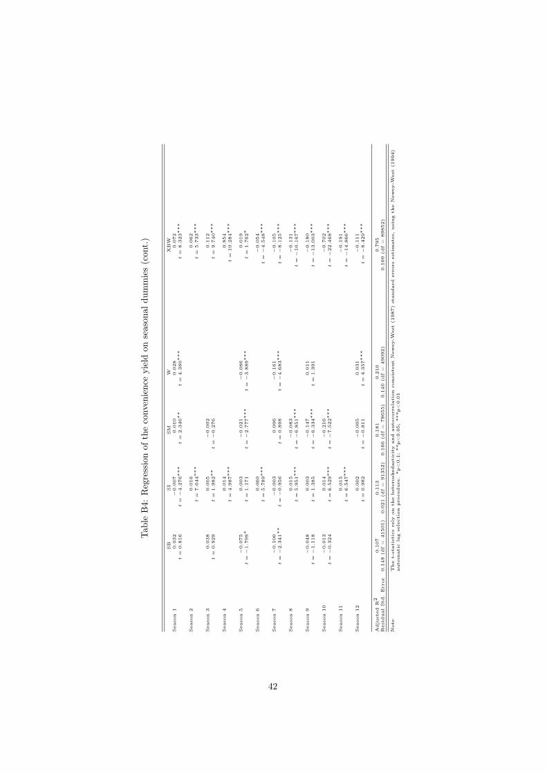
42

Tab

le B

4: R



al dum

mies (con

t.)

SB

SI

SM

W

XBW

Season 1

0.032

−0.007

0.010

0.028

0.072

t

=0.816

t

= −4.276∗∗∗

t

=2.346∗∗

t

=4.380∗∗∗

t

=8.323∗∗∗

Season 2

0.016

0.062

t

=

t =

7.644∗∗∗

5.733∗∗∗

Season 3

0.038

0.005

−0.002

0.112

t

=0.929

t

=1.982∗∗

t

= −0.276

t

=9.740∗∗∗

Season 4

0.014

0.854

t

=

t =

4.987∗∗∗

10.284∗∗∗

Season 5

−0.075

0.003

−0.021

−0.086

0.019

t

= −1.799∗

t

=1.171

t

= −2.777∗∗∗

t

= −3.889∗∗∗

t

=1.762∗

Season 6

0.060

−0.054

t

=

t =

5.789∗∗∗

−4.548∗∗∗

Season 7

−0.100

−0.003

0.006

−0.161

−0.105

t

= −2.341∗∗

t

= −0.956

t

=0.898

t

= −4.683∗∗∗

t

= −8.125∗∗∗

Season 8

0.015

−0.083

−0.131

t

=

t =

t

=5.951∗∗∗

−6.851∗∗∗

−10.167∗∗∗

Season 9

−0.048

0.003

−0.147

0.011

−0.180

t

= −1.118

t

=1.385

t

= −6.334∗∗∗

t

=1.391

t

= −13.003∗∗∗

Season 10

−0.013

0.014

−0.216

−0.702

t

= −0.324

t

=6.529∗∗∗

t

= −7.522∗∗∗

t

= −22.468∗∗∗

Season 11

0.015

−0.191

t

=

t =

6.547∗∗∗

−14.866∗∗∗

Season 12

0.002

−0.005

0.031

−0.111

t

=0.982

t

= −0.811

t

=4.357∗∗∗

t

= −8.429∗∗∗

Adjusted R2

0.107

0.113

0.181

0.210

0.795

Residual Std. Error

0.148 (df = 41501)

0.021 (df = 91352)

0.166 (df = 78655)

0.140 (df = 49092)

0.169 (df = 89852)

Note


ey-W


ates, using the New

ey-W

est (1994)


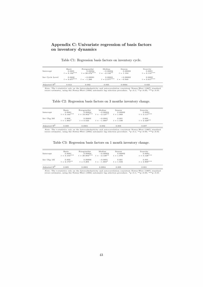
Appendix C: Univariate regression of basis factors on inventory dynamics

Table C1: Regression basis factors on inventory cycle.


t = 3.132 ∗∗∗

ForegoneInt 0.00004

t = 20.072 ∗∗∗

Median −0.00004

t = −2.132 ∗∗

Season 0.00002

t = 1.104

Scarcity 0.0001

t = 3.110 ∗∗∗

Inv Cycle Level 0.0002 t = 3.677 ∗∗∗

−0.00001 t = −1.266

0.00001 t = 2.577 ∗∗∗

−0.00002 t = −0.940

0.0002 t = 3.617 ∗∗∗

Adjusted R2 0.013 0.002 0.005 0.0004 0.025


Table C2: Regression basis factors on 3 months inventory change.


t = 3.144 ∗∗∗

ForegoneInt 0.00004

t = 19.952 ∗∗∗

Median −0.00004

t = −2.127 ∗∗

Season 0.00002

t = 1.069

Scarcity 0.0001

t = 3.117 ∗∗∗

Inv Chg 3M 0.002 t = 1.894 ∗

0.00001 t = 0.523

−0.0001 t = −1.900 ∗

0.001 t = 1.199

0.001 t = 2.429 ∗∗

Adjusted R2 0.009 0.0001 0.002 0.003 0.007


Table C3: Regression basis factors on 1 month inventory change.


t = 3.153 ∗∗∗

ForegoneInt 0.00004

t = 20.003 ∗∗∗

Median −0.00004

t = −2.128 ∗∗

Season 0.00002

t = 1.078

Scarcity 0.0001

t = 3.128 ∗∗∗

Inv Chg 1M 0.002 t = 2.173 ∗∗

0.00000 t = 0.265

−0.0001 t = −1.804 ∗

0.001 t = 1.534

0.001 t = 2.899 ∗∗∗

Adjusted R2 0.005 0.0001 0.0004 0.005 0.001


43

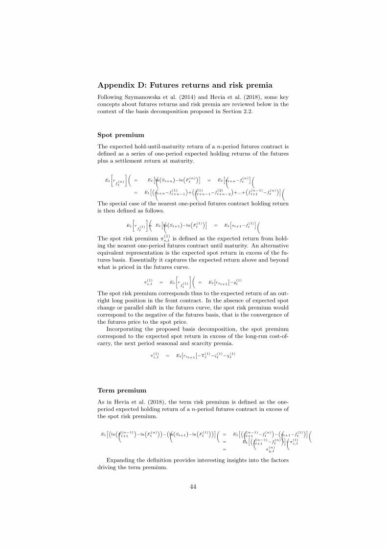
Appendix D: Futures returns and risk premia Following Szymanowska et al. (2014) and Hevia et al. (2018), some key concepts about futures returns and risk premia are reviewed below in the context of the basis decomposition proposed in Section 2.2.

Spot premium

The expected hold-until-maturity return of a n-period futures contract is defned as a series of one-period expected holding returns of the futures plus a settlement return at maturity.

" # h � �i h i (n) (n)

Et r = Et ln(St+n)−ln F = Et st+n−f f(n) t t t h� � � � � �i

(1) (1) (2) (n−1) (n)= Et st+n−f + f −f +...+ f −f t+n−1 t+n−1 t+n−2 t+1 t

The special case of the nearest one-period futures contract holding return is then defned as follows.

" # h � �i h i (1) (1)

Et r = Et ln(St+1 )−ln F = Et st+1 −f(1) t tf t

(1)The spot risk premium πs,t is defned as the expected return from hold-ing the nearest one-period futures contract until maturity. An alternative equivalent representation is the expected spot return in excess of the fu-tures basis. Essentially it captures the expected return above and beyond what is priced in the futures curve.

" # (1) (1)

π = Et r = ]−ys,t (1) Et[rst+1 tf t

The spot risk premium corresponds thus to the expected return of an out-right long position in the front contract. In the absence of expected spot change or parallel shift in the futures curve, the spot risk premium would correspond to the negative of the futures basis, that is the convergence of the futures price to the spot price.

Incorporating the proposed basis decomposition, the spot premium correspond to the expected spot return in excess of the long-run cost-of-carry, the next period seasonal and scarcity premia.

(1) (1) (1) (1) s,t Et[rst+1 t t tπ = ]− −ζ −χ

Term premium

As in Hevia et al. (2018), the term risk premium is defned as the one-period expected holding return of a n-period futures contract in excess of the spot risk premium.

h� � � � �� i h� � � �i (n−1) (n) (1) (n−1) (n) (1)

Et ln F −ln F − ln(St+1)−ln F = Et f −f − t+1 t t t+1 t st+1−fth� �i (n−1) (n) (1) t+1 t s,t = Et f −f −π

(n)= πy,t

Expanding the defnition provides interesting insights into the factors driving the term premium.

44

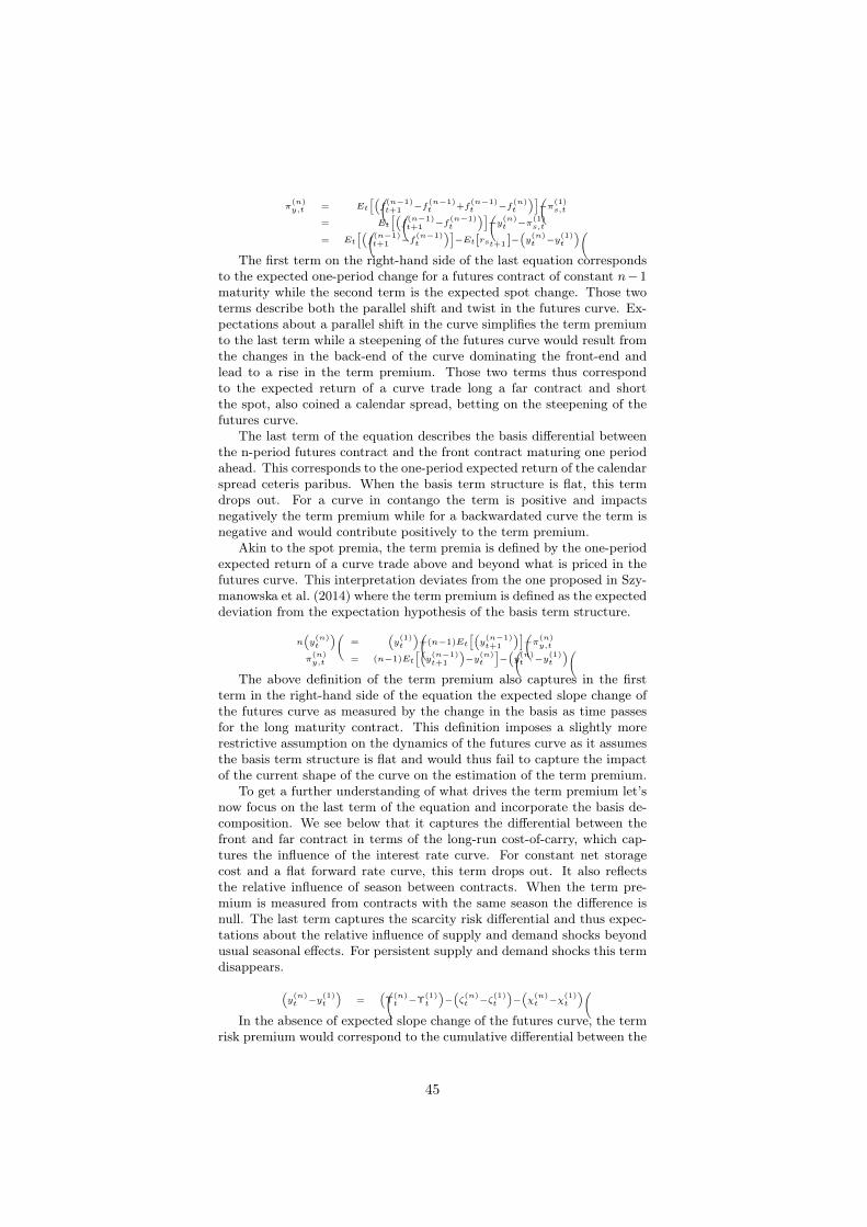
h� �i (n) (n−1) (n−1) (n−1) (n) (1)

π = f −f +f −f −πy,t Et t+1 t t t s,th� �i (n−1) (n−1) (n) (1)

= f −f −y −πEt t+1 t t s,th� �i � � (n−1) (n−1) (n) (1)

= Et f −ft ]− y −ytt+1 −Et[rst+1 t

The frst term on the right-hand side of the last equation corresponds to the expected one-period change for a futures contract of constant n − 1 maturity while the second term is the expected spot change. Those two terms describe both the parallel shift and twist in the futures curve. Ex-pectations about a parallel shift in the curve simplifes the term premium to the last term while a steepening of the futures curve would result from the changes in the back-end of the curve dominating the front-end and lead to a rise in the term premium. Those two terms thus correspond to the expected return of a curve trade long a far contract and short the spot, also coined a calendar spread, betting on the steepening of the futures curve.

The last term of the equation describes the basis di˙erential between the n-period futures contract and the front contract maturing one period ahead. This corresponds to the one-period expected return of the calendar spread ceteris paribus. When the basis term structure is fat, this term drops out. For a curve in contango the term is positive and impacts negatively the term premium while for a backwardated curve the term is negative and would contribute positively to the term premium.

Akin to the spot premia, the term premia is defned by the one-period expected return of a curve trade above and beyond what is priced in the futures curve. This interpretation deviates from the one proposed in Szy-manowska et al. (2014) where the term premium is defned as the expected deviation from the expectation hypothesis of the basis term structure.

� � � � h� �i (n) (1) (n−1) (n)

n y = y +(n−1)Et y −πt t t+1 y,t h� � i � � (n) (n−1) (n) (n) (1)

π = (n−1)Et y −y − y −yy,t t+1 t t t

The above defnition of the term premium also captures in the frst term in the right-hand side of the equation the expected slope change of the futures curve as measured by the change in the basis as time passes for the long maturity contract. This defnition imposes a slightly more restrictive assumption on the dynamics of the futures curve as it assumes the basis term structure is fat and would thus fail to capture the impact of the current shape of the curve on the estimation of the term premium.

To get a further understanding of what drives the term premium let’s now focus on the last term of the equation and incorporate the basis de-composition. We see below that it captures the di˙erential between the front and far contract in terms of the long-run cost-of-carry, which cap-tures the infuence of the interest rate curve. For constant net storage cost and a fat forward rate curve, this term drops out. It also refects the relative infuence of season between contracts. When the term pre-mium is measured from contracts with the same season the di˙erence is null. The last term captures the scarcity risk di˙erential and thus expec-tations about the relative infuence of supply and demand shocks beyond usual seasonal e˙ects. For persistent supply and demand shocks this term disappears.

� � � � � � � � (n) (1) (n) (1) (n) (1) (n) (1)

y −y = − − ζ −ζ − χ −χt t t t t t t t

In the absence of expected slope change of the futures curve, the term risk premium would correspond to the cumulative di˙erential between the

45

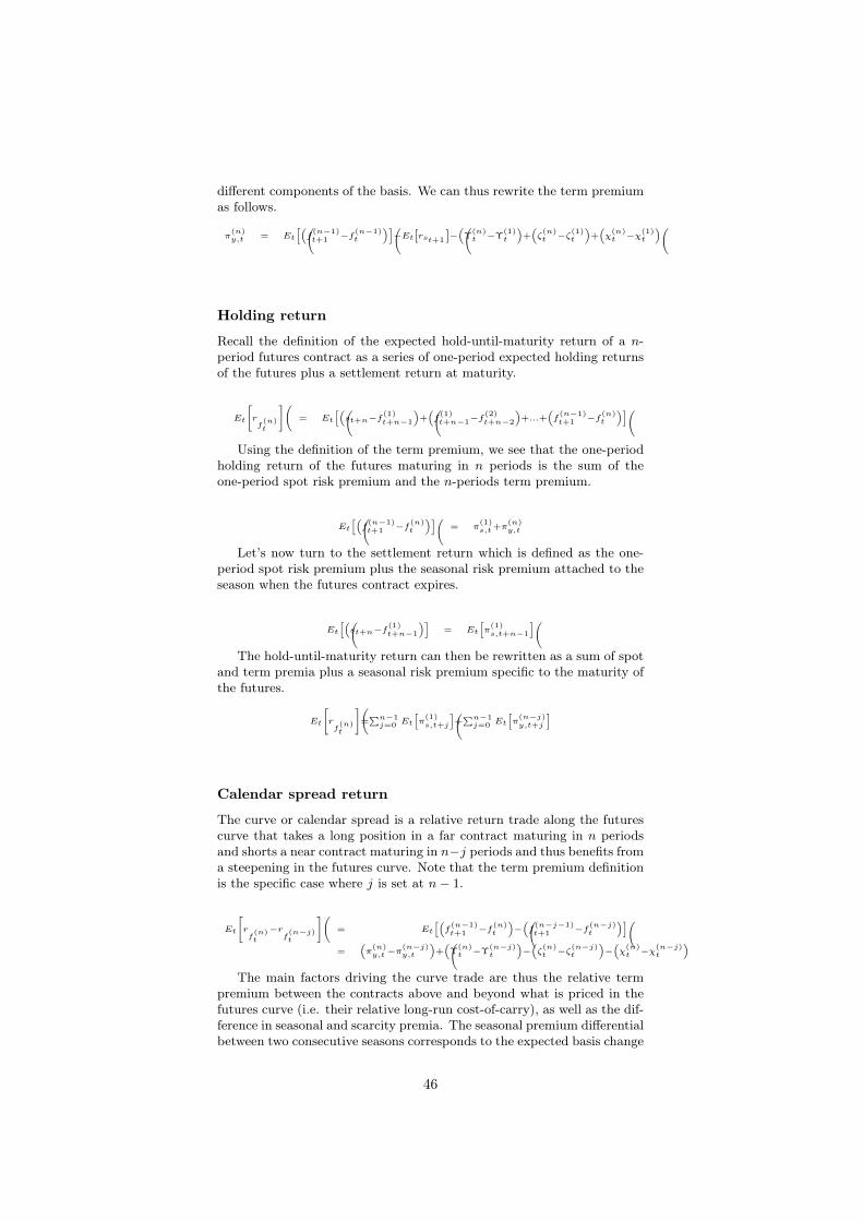
di˙erent components of the basis. We can thus rewrite the term premium as follows.

h� �i � � � � � � (n) (n−1) (n−1) (n) (1) (n) (1) (n) (1)

π = Et f −f ]− − + ζ −ζ + χ −χy,t t+1 t −Et[rst+1 t t t t t t

Holding return

Recall the defnition of the expected hold-until-maturity return of a n-period futures contract as a series of one-period expected holding returns of the futures plus a settlement return at maturity.

" # h� � � � � �i (1) (1) (2) (n−1) (n)

Et r = Et st+n−f + f −f +...+ f −f(n) t+n−1 t+n−1 t+n−2 t+1 tft

Using the defnition of the term premium, we see that the one-period holding return of the futures maturing in n periods is the sum of the one-period spot risk premium and the n-periods term premium.

h� �i (n−1) (n) (1) (n)

Et f −f = π +π t+1 t s,t y,t

Let’s now turn to the settlement return which is defned as the one-period spot risk premium plus the seasonal risk premium attached to the season when the futures contract expires.

h� �i h i (1) (1)

Et st+n−f = Et π t+n−1 s,t+n−1

The hold-until-maturity return can then be rewritten as a sum of spot and term premia plus a seasonal risk premium specifc to the maturity of the futures.

" # h i h iPn−1 (1) Pn−1 (n−j)Et r = Et π + Et π

f (n) j=0 s,t+j j=0 y,t+j t

Calendar spread return

The curve or calendar spread is a relative return trade along the futures curve that takes a long position in a far contract maturing in n periods and shorts a near contract maturing in n−j periods and thus benefts from a steepening in the futures curve. Note that the term premium defnition is the specifc case where j is set at n − 1.

" # h� � � �i (n−1) (n) (n−j−1) (n−j)

Et r −r = Et f −f − f −f(n) (n−j) t+1 t t+1 tf f � � � � � � � �t t (n) (n−j) (n) (n−j) (n) (n−j) (n) (n−j)

= π −π + − − ζ −ζ − χ −χy,t y,t t t t t t t

The main factors driving the curve trade are thus the relative term premium between the contracts above and beyond what is priced in the futures curve (i.e. their relative long-run cost-of-carry), as well as the dif-ference in seasonal and scarcity premia. The seasonal premium di˙erential between two consecutive seasons corresponds to the expected basis change

46

resulting from the dynamics of supply and demand imbalances across sea-sons and is driven by the change in inventory levels. The scarcity premium di˙erential captures the expected normalization of unexpected supply or demand shocks over that period. Appendix E investigates the infuence of the various factors driving the basis on the calendar spread return.

47

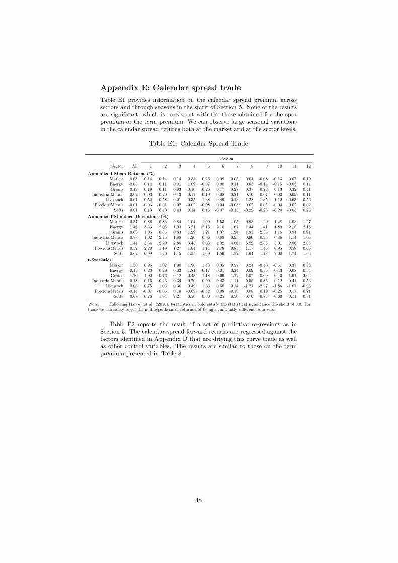
Appendix E: Calendar spread trade Table E1 provides information on the calendar spread premium across sectors and through seasons in the spirit of Section 5. None of the results are signifcant, which is consistent with the those obtained for the spot premium or the term premium. We can observe large seasonal variations in the calendar spread returns both at the market and at the sector levels.

Table E1: Calendar Spread Trade

Season

Sector All 1 2 3 4 5 6 7 8 9 10 11 12

Annualized Mean Returns (%) Market 0.08 0.14 0.14 0.14 0.34 0.26 0.09 0.05 0.04 -0.08 -0.13 0.07 0.19 Energy -0.03 0.14 0.11 0.01 1.09 -0.07 0.00 0.11 0.03 -0.14 -0.15 -0.03 0.14 Grains 0.19 0.19 0.11 0.03 0.10 0.26 0.17 0.27 0.37 0.28 0.13 0.32 0.41

IndustrialMetals 0.02 0.03 -0.20 -0.13 0.17 0.19 0.08 0.21 0.10 0.07 0.02 0.09 0.11 Livestock 0.01 0.52 0.58 0.21 0.35 1.38 0.49 0.13 -1.28 -1.35 -1.12 -0.63 -0.56

PreciousMetals -0.01 -0.03 -0.01 0.02 -0.02 -0.08 0.04 -0.03 0.02 0.05 -0.04 0.02 0.02 Softs 0.01 0.13 0.40 0.43 0.14 0.15 -0.07 -0.13 -0.22 -0.25 -0.20 -0.03 0.23

Annualized Standard Deviations (%) Market 0.37 0.86 0.83 0.84 1.04 1.09 1.53 1.05 0.98 1.20 1.48 1.08 1.27 Energy 1.46 3.33 2.05 1.93 3.21 2.16 2.10 1.67 1.44 1.41 1.89 2.18 2.18 Grains 0.68 1.05 0.85 0.83 1.29 1.21 1.37 1.24 1.93 2.33 1.76 0.94 0.91

IndustrialMetals 0.73 1.02 2.25 1.88 1.20 0.96 0.89 0.93 0.90 0.95 0.86 1.14 1.05 Livestock 1.44 3.34 2.79 2.80 3.45 5.03 4.02 4.66 5.22 2.88 3.01 2.86 2.85

PreciousMetals 0.32 2.20 1.19 1.27 1.04 1.14 2.78 0.85 1.17 1.46 0.95 0.58 0.66 Softs 0.62 0.99 1.20 1.15 1.55 1.69 1.56 1.52 1.64 1.73 2.00 1.74 1.66

t-Statistics Market 1.30 0.95 1.02 1.00 1.90 1.43 0.35 0.27 0.24 -0.40 -0.51 0.37 0.88 Energy -0.13 0.23 0.29 0.03 1.81 -0.17 0.01 0.34 0.09 -0.55 -0.43 -0.08 0.34 Grains 1.70 1.00 0.76 0.18 0.43 1.18 0.69 1.22 1.07 0.69 0.40 1.91 2.64

IndustrialMetals 0.18 0.16 -0.43 -0.34 0.70 0.99 0.43 1.11 0.55 0.36 0.12 0.41 0.53 Livestock 0.06 0.75 1.03 0.36 0.49 1.33 0.60 0.14 -1.21 -2.27 -1.86 -1.07 -0.96

PreciousMetals -0.14 -0.07 -0.05 0.10 -0.09 -0.42 0.08 -0.19 0.08 0.19 -0.25 0.17 0.21 Softs 0.08 0.76 1.94 2.21 0.50 0.50 -0.25 -0.50 -0.76 -0.83 -0.60 -0.11 0.81

Note: Following Harvey et al. (2016), t-statistics in bold satisfy the statistical signifcance threshold of 3.0. For those we can safely reject the null hypothesis of returns not being signifcantly di˙erent from zero.

Table E2 reports the result of a set of predictive regressions as in Section 5. The calendar spread forward returns are regressed against the factors identifed in Appendix D that are driving this curve trade as well as other control variables. The results are similar to those on the term premium presented in Table 8.

48

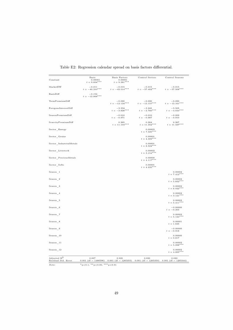
Table E2: Regression calendar spread on basis factors di˙erential.

Basis Basis Factors Control Sectors Control Seasons Constant 0.00001 0.00001

t = t =9.604 ∗∗∗ 9.381 ∗∗∗

MarketEW −0.011 −0.015 −0.015 −0.015 t = t = t = t =−40.310 ∗∗∗ −43.514 ∗∗∗ −57.402 ∗∗∗ −57.508 ∗∗∗

BasisDi˙ −0.154 t = −12.808 ∗∗∗

TermPremiumDi˙ −0.090 −0.090 −0.090 t = t = t =−12.134 ∗∗∗ −13.157 ∗∗∗ −13.161 ∗∗∗

ForegoneInterestDi˙ −3.334 −3.245 −3.505 t = t = t =−3.828 ∗∗∗ −3.760 ∗∗∗ −4.034 ∗∗∗

SeasonPremiumDi˙ −0.010 −0.010 −0.009 t = −0.971 t = −0.987 t = −0.910

ScarcityPremiumDi˙ 0.265 0.264 0.267 t = t = t =11.104 ∗∗∗ 11.352 ∗∗∗ 11.437 ∗∗∗

Sector_Energy 0.00003 t = 7.325 ∗∗∗

Sector_Grains 0.00001 t = 4.309 ∗∗∗

Sector_IndustrialMetals 0.00001 t = 8.502 ∗∗∗

Sector_Livestock 0.00002 t = 3.154 ∗∗∗

Sector_PreciousMetals 0.00000 t = 4.117 ∗∗∗

Sector_Softs 0.00001 t = 4.235 ∗∗∗

Season_1 0.00002 t = 7.412 ∗∗∗

Season_2 0.00002 t = 5.832 ∗∗∗

Season_3 0.00002 t = 6.022 ∗∗∗

Season_4 0.00002 t = 3.121 ∗∗∗

Season_5 0.00002 t = 5.411 ∗∗∗

Season_6 −0.00000 t = −0.355

Season_7 0.00002 t = 5.124 ∗∗∗

Season_8 0.00001 t = 1.635

Season_9 −0.00000 t = −0.918

Season_10 0.00000 t = 0.817

Season_11 0.00002 t = 5.098 ∗∗∗

Season_12 0.00002 t = 4.895 ∗∗∗

Adjusted R2 0.007 0.020 0.020 0.020 Residual Std. Error 0.001 (df = 1486596) 0.001 (df = 1265355) 0.001 (df = 1265350) 0.001 (df = 1265344)

∗Note: p<0.1; ∗∗ p<0.05; ∗∗∗ p<0.01

49

�

References

Bakshi, G., Gao, X. and Rossi, A. G. (2017), ‘Understanding the sources of risk underlying the cross section of commodity returns’, Management Science 65(2), 619–641. 5.1, 5.1

Borovkova, S. and Geman, H. (2006), ‘Seasonal and stochastic e˙ects in commodity forward curves’, Review of Derivatives Research 9(2), 167– 186. 1.2, 6

Brennan, M. J. (1958), ‘The supply of storage’, The American Economic Review pp. 50–72. 1.2

Brooks, C., Prokopczuk, M. and Wu, Y. (2013), ‘Commodity futures prices: More evidence on forecast power, risk premia and the theory of storage’, The Quarterly Review of Economics and Finance 53(1), 73– 85. 1.2

Campbell, J. Y. and Shiller, R. J. (1988), ‘Stock prices, earnings, and expected dividends’, The Journal of Finance 43(3), 661–676. 2.2

Chordia, T., Goyal, A. and Saretto, A. (2017), ‘p-hacking: Evidence from two million trading strategies’, Swiss Finance Institute Research Paper No. 17-37 . 10

Deaton, A. and Laroque, G. (1992), ‘On the behaviour of commodity prices’, The Review of Economic Studies 59(1), 1–23. 1.1, 1.2

Fama, E. F. and French, K. R. (1987), ‘Commodity futures prices: Some evidence on forecast power, premiums, and the theory of storage’, Jour-nal of Business pp. 55–73. 1.1, 1.2, 2

French, K. R. (1986), ‘Detecting spot price forecasts in futures prices’, Journal of Business pp. S39–S54. 1.2

Geman, H. and Nguyen, V.-N. (2005), ‘Soybean inventory and forward curve dynamics’, Management Science 51(7), 1076–1091. 1.2

Gorton, G. B., Hayashi, F. and Rouwenhorst, K. G. (2013), ‘The funda-mentals of commodity futures returns’, Review of Finance 17(1), 35– 105. 1.1, 4, 3.3, 9, 4.1, 6.3

Hamilton, J. D. (2017), ‘Why you should never use the hodrick-prescott flter’, The Review of Economics and Statistics 100(5), 831–843. 3.3

Hannan, E. J., Terrell, R. and Tuckwell, N. (1970), ‘The seasonal ad-justment of economic time series’, International Economic Review 11(1), 24–52. 1.2, 6

Harvey, C. R. (2017), ‘Presidential address: The scientifc outlook in f-nancial economics’, The Journal of Finance 72(4), 1399–1440. 10

Harvey, C. R. and Liu, Y. (2015), ‘Backtesting’, The Journal of Portfolio Management 42(1), 13–28. 10

50

Harvey, C. R., Liu, Y. and Zhu, H. (2016), ‘... and the cross-section of expected returns’, The Review of Financial Studies 29(1), 5–68. 10, 3.5, 5.1, 6.3

Hausman, J. A. (1978), ‘Specifcation tests in econometrics’, Econometrica pp. 1251–1271. 4.1

Hevia, C., Petrella, I. and Sola, M. (2018), ‘Risk premia and seasonality in commodity futures’, Journal of Applied Econometrics 33(6), 853–873. 1.1, 1.2, 6, 6.3

Hirshleifer, D. (1991), ‘Seasonal patterns of futures hedging and the res-olution of output uncertainty’, Journal of economic theory 53(2), 304– 327. 1.2, 16

Hirshleifer, D. (2001), ‘Investor Psychology and Asset Pricing’, The Jour-nal of Finance 56(4), 1533–1597. 13

Hong, H., Lim, T. and Stein, J. C. (2000), ‘Bad news travels slowly: Size, analyst coverage, and the proftability of momentum strategies’, The Journal of Finance 55(1), 265–295. 12, 15

Hong, H. and Stein, J. C. (1999), ‘A unifed theory of underreaction, momentum trading, and overreaction in asset markets’, The Journal of Finance 54(6), 2143–2184. 12, 15

Hou, K., Xue, C. and Zhang, L. (2015), ‘Digesting anomalies: An in-vestment approach’, The Review of Financial Studies 28(3), 650–705. 10

Hou, K., Xue, C. and Zhang, L. (2017), ‘Replicating anomalies’, Fisher College of Business working paper No. 2017-03-010 (23394). 10

Jegadeesh, N. and Titman, S. (1993), ‘Returns to buying winners and selling losers: Implications for stock market eÿciency’, The Journal of Finance 48(1), 65–91. 12

Kaldor, N. (1939), ‘Speculation and economic stability’, The Review of Economic Studies 7(1), 1–27. 1.1

Keloharju, M., Linnainmaa, J. T. and Nyberg, P. (2016), ‘Return season-alities’, The Journal of Finance 71(4), 1557–1590. 1.2, 6.3

Koijen, R. S. J., Moskowitz, T. J., Pedersen, L. H. and Vrugt, E. B. (2018), ‘Carry’, Journal of Financial Economics 127(2), 197–225. 1

Linnainmaa, J. T. and Roberts, M. R. (2018), ‘The history of the cross-section of stock returns’, The Review of Financial Studies 31(7), 2606– 2649. 10

Malkiel, B. G. and Fama, E. F. (1970), ‘Eÿcient capital markets: A review of theory and empirical work’, The Journal of Finance 25(2), 383–417. 11

Newey, W. K. and West, K. (1994), ‘Automatic Lag Selection in Covari-ance Matrix Estimation’, Review of Economic Studies 61(4), 631–653. 4.1, 5.1

51

Newey, W. K. and West, K. D. (1987), ‘A simple, positive semi-defnite, heteroskedasticity and autocorrelation consistent covariance matrix.’, Econometrica 55(3), 703. 4.1, 5.1

Routledge, B. R., Seppi, D. J. and Spatt, C. S. (2000), ‘Equilibrium for-ward curves for commodities’, The Journal of Finance 55(3), 1297– 1338. 1.1, 4

Shleifer, A. and Vishny, R. W. (1997), ‘The Limits of Arbitrage’, The Journal of Finance 52(1), 35–55. 14

Sørensen, C. (2002), ‘Modeling seasonality in agricultural commodity fu-tures’, Journal of Futures Markets 22(5), 393–426. 1.2, 6

Szymanowska, M., Roon, F., Nijman, T. and Goorbergh, R. (2014), ‘An anatomy of commodity futures risk premia’, The Journal of Finance 69(1), 453–482. 1.1, 6.3

Telser, L. G. (1958), ‘Futures trading and the storage of cotton and wheat’, The Journal of Political Economy pp. 233–255. 1.2

Working, H. (1948), ‘Theory of the inverse carrying charge in futures markets’, Journal of Farm Economics 30(1), 1–28. 1.1

52

Scarcity risk Premium - Lancaster University

Documents

Transcript of Scarcity risk Premium - Lancaster University