Multichannel Azimuth Processing in ScanSAR and TOPS Mode ...

SCANSAR-TO-STRIPMAP INTERFEROMETRIC OBSERVATIONS OF
HAWAII
A DISSERTATION
SUBMITTED TO THE DEPARTMENT OF ELECTRICAL
ENGINEERING
AND THE COMMITTEE ON GRADUATE STUDIES
OF STANFORD UNIVERSITY
IN PARTIAL FULFILLMENT OF THE REQUIREMENTS
FOR THE DEGREE OF
DOCTOR OF PHILOSOPHY
Ana Bertran Ortiz
September 2007

© Copyright by Ana Bertran Ortiz 2007
All Rights Reserved
ii

I certify that I have read this dissertation and that, in my opinion, it is fully
adequate in scope and quality as a dissertation for the degree of Doctor of
Philosophy.
(Howard A. Zebker) Principal Adviser
I certify that I have read this dissertation and that, in my opinion, it is fully
adequate in scope and quality as a dissertation for the degree of Doctor of
Philosophy.
(Ivan Linscott)
I certify that I have read this dissertation and that, in my opinion, it is fully
adequate in scope and quality as a dissertation for the degree of Doctor of
Philosophy.
(John M. Pauly)
Approved for the University Committee on Graduate Studies.
iii

Abstract
InSAR images of geophysical events such as pre-eruptive volcano deformation or inter-
seismic strain accumulation are often limited by phase distortions from the superimposed
atmospheric signature. Additionally, the approximate monthly repeat cycle of many radar
satellites cannot accurately capture rapidly time-varying processes. The ScanSAR mode
of the Envisat ASAR instrument permits more frequent revisits of a given area, poten-
tially overcoming both of these limitations. In particular, stripmap-to-ScanSAR images
provide a denser time series of interferograms than is possible with conventional stripmap-
to-stripmap InSAR.
In this work we develop a method to generate efficiently scanSAR-to-stripmap interfer-
ograms. We present a time series of Envisat data acquired over Hawaii in which ScanSAR
mode data are combined with Envisat conventional stripmap mode data to form a series of
interferograms at a denser temporal spacing than is possible with normal InSAR.
The burst nature of ScanSAR data and the differences in the pulse repetition frequency
between the two modes require a new processing method to formthe interferograms. We
use traditional matched filtering for the range compression. For the azimuth processing,
we compute the stripmap mode data on the ScanSAR sampling grid using a variation,
consisting of different reference functions to readjust the azimuth pulse spacing, of Lanari’s
modified SPECAN algorithm, itself an adaptation of the chirp-z transform. Additionally,
we present a method for the co-registration of stripmap datato ScanSAR data. For the fine
co-registration we use the linear relation between the phase ramp present across a burst in
misregistered stripmap-to-ScanSAR interferograms and the misregistration amount.
The resulting interferograms faithfully reflect the phase of conventional interferograms,
but exhibit fewer looks and coarser resolution than those produced by fully stripmap mode
iv

data. For many problems temporal density of the deformationobservations is paramount,
and the time series analysis and temporal averaging made possible using ScanSAR inter-
ferograms far outweighs the loss in looks and resolution.
v

Acknowledgements
I would like to take this opportunity to thank all of those whohave helped me make this
dissertation possible.
First and foremost, I would like to offer my sincere and deep gratitude to my adviser
Howard Zebker. He has offered me generous and extremely valuable guidance and support
throughout the whole process. He has kept me focused and I will be forever grateful. I
would like to thank Dr. Ivan Linscott and John M. Pauly for valuable advice and for being
second and third readers, the later also for charing my oral defense. I thank Donald C. Cox
and G. Leonard Tyler for their valuable comments during my oral defense and for their
support. Additionally, I would like to thank Paul Rosen and Scott Hensley from JPL for
very helpful discussions.
I am proud to have been a part of the Radar Interferometry Group at Stanford University.
I have shared many valuable academic and non-academic discussions with its current and
past members: Dr. Leif Harcke, Dr. Andy Hooper, Dr. Fayaz Onn, Dr. Noa Bechor,
Dr. Sang-Ho Yun, Shadi Oveisgharan, Lauren Wye, Piyush Shanker and Albert Chen. My
sincere gratitude to all and I look forward to continuing discussions.
I would like to thank the other members of Packard who have made the years here an
important and fun part of my live. In particular, I would liketo thank professor Antony C.
Fraser-Smith, among other things, for his continuous supply of research-relevant magazines
and for his support. Many thanks to Kamakshi, Cecile, Tim, Deirdre, Sarah, Cristina,
Fraser, Hrefna, Bob, Erin and Kerri. It has been a blast to be apart of Packard and I will
cherish my years here.
I have been fortunate to receive the support of many friends outside of Stanford. I thank
Erika, Genti, Curtis, Matt, Jorge and Suelika, Eric and Jackie, Dave and Darci, Marisol and
vi

Luis, Ylan and Orly, Yuka, Maria and John T. Thanks for your continuous support.
This research was conducted under contract with National Aeronautics and Space Ad-
ministration (NASA) and the National Science Foundation (NSF). I also acknowledge the
European Space Agency (ESA) for supplying the raw data from the Envisat ASAR satel-
lite through the WinSAR project. This research was possiblethanks to the support of the
aforementioned organizations.
Finally, none of this would have been possible without the unwavering support of my
husband, Roberto Angulo, my sister Nuria Bertran and my parents Francisco Bertran and
Maria Dolores Ortiz. To my husband, I know I can always count on you and for that I feel
really lucky.
vii

Contents
Abstract iv
Acknowledgements vi
List of Symbols xxii
1 Motivation 1
1.1 Introduction . . . . . . . . . . . . . . . . . . . . . . . . . . . . . . . . . . 1
1.2 Objectives . . . . . . . . . . . . . . . . . . . . . . . . . . . . . . . . . . . 9
1.3 Contributions . . . . . . . . . . . . . . . . . . . . . . . . . . . . . . . . . 10
2 InSAR 12
2.1 Introduction . . . . . . . . . . . . . . . . . . . . . . . . . . . . . . . . . . 12
2.2 SAR . . . . . . . . . . . . . . . . . . . . . . . . . . . . . . . . . . . . . . 13
2.2.1 Doppler history of a point target . . . . . . . . . . . . . . . . . .. 16
2.2.2 Typical processing . . . . . . . . . . . . . . . . . . . . . . . . . . 18
2.2.3 Doppler centroid . . . . . . . . . . . . . . . . . . . . . . . . . . . 20
2.2.4 Range cell migration . . . . . . . . . . . . . . . . . . . . . . . . . 23
2.3 Interferometric SAR . . . . . . . . . . . . . . . . . . . . . . . . . . . . . 24
2.4 Limitations of InSAR . . . . . . . . . . . . . . . . . . . . . . . . . . . . . 27
2.5 Conclusions . . . . . . . . . . . . . . . . . . . . . . . . . . . . . . . . . . 29
3 The Envisat satellite 30
3.1 Introduction . . . . . . . . . . . . . . . . . . . . . . . . . . . . . . . . . . 30
viii

3.2 Advanced synthetic aperture radar (ASAR) . . . . . . . . . . . .. . . . . 30
3.2.1 ASAR stripmap mode . . . . . . . . . . . . . . . . . . . . . . . . 31
3.2.2 ASAR ScanSAR mode . . . . . . . . . . . . . . . . . . . . . . . . 32
3.3 ASAR parameters . . . . . . . . . . . . . . . . . . . . . . . . . . . . . . . 35
3.4 Conclusion . . . . . . . . . . . . . . . . . . . . . . . . . . . . . . . . . . 36
4 Azimuth processing of burst-mode SAR data 38
4.1 Introduction . . . . . . . . . . . . . . . . . . . . . . . . . . . . . . . . . . 38
4.2 Algorithms for processing stripmap SAR data . . . . . . . . . .. . . . . . 39
4.2.1 Range-Doppler . . . . . . . . . . . . . . . . . . . . . . . . . . . . 39
4.2.2 Chirp scaling algorithm . . . . . . . . . . . . . . . . . . . . . . . 39
4.3 Doppler history of a point target in burst mode . . . . . . . . .. . . . . . . 43
4.4 Algorithms for ScanSAR data. . . . . . . . . . . . . . . . . . . . . . . .. 44
4.4.1 Traditional InSAR with zero padded data . . . . . . . . . . . .. . 44
4.4.2 The spectral analysis, or SPECAN, method . . . . . . . . . . .. . 45
4.4.3 Modified SPECAN . . . . . . . . . . . . . . . . . . . . . . . . . . 46
4.4.4 Extended chirp scaling . . . . . . . . . . . . . . . . . . . . . . . . 48
4.4.5 Our method for processing Envisat data . . . . . . . . . . . . .. . 49
4.5 Conclusions . . . . . . . . . . . . . . . . . . . . . . . . . . . . . . . . . . 50
5 Stripmap-to-ScanSAR processing 51
5.1 Introduction . . . . . . . . . . . . . . . . . . . . . . . . . . . . . . . . . . 51
5.2 Variation of the modified SPECAN . . . . . . . . . . . . . . . . . . . . .. 51
5.3 Processing steps . . . . . . . . . . . . . . . . . . . . . . . . . . . . . . . . 54
5.3.1 Co-registering the stripmap image to the ScanSar image . . . . . . 56
5.3.2 Deramping and chirp-z transform . . . . . . . . . . . . . . . . . .58
5.3.3 Azimuth ramps . . . . . . . . . . . . . . . . . . . . . . . . . . . . 63
5.4 Conclusions . . . . . . . . . . . . . . . . . . . . . . . . . . . . . . . . . . 64
6 Two case studies 65
6.1 Introduction . . . . . . . . . . . . . . . . . . . . . . . . . . . . . . . . . . 65
6.2 Two case studies . . . . . . . . . . . . . . . . . . . . . . . . . . . . . . . 65
ix

6.3 Proof of concept . . . . . . . . . . . . . . . . . . . . . . . . . . . . . . . . 66
6.4 Conclusions . . . . . . . . . . . . . . . . . . . . . . . . . . . . . . . . . . 71
7 Data series of interferograms 72
7.1 Introduction . . . . . . . . . . . . . . . . . . . . . . . . . . . . . . . . . . 72
7.2 Selection of interferometric pairs . . . . . . . . . . . . . . . . .. . . . . . 72
7.3 Data series . . . . . . . . . . . . . . . . . . . . . . . . . . . . . . . . . . . 73
7.4 Interferogram stack for atmospheric compensation . . . .. . . . . . . . . 75
7.5 Conclusion . . . . . . . . . . . . . . . . . . . . . . . . . . . . . . . . . . 79
8 Conclusions 86
8.1 Contributions . . . . . . . . . . . . . . . . . . . . . . . . . . . . . . . . . 86
8.2 Future directions . . . . . . . . . . . . . . . . . . . . . . . . . . . . . . . 88
A Chirp scaling algorithm 89
B Phase ramp in ScanSAR 92
C Phase ramp in burst-mode with squinted geometry 94
Bibliography 99
x

List of Tables
3.1 Key Parameters of those ENVISAT/ASAR beams usable for stripmap-to-
ScanSAR interferometry. Each stripmap beam has been placednext to its
ScanSAR counterpart.NB is the number of pulses in one burst andNR is
the number of pulses in one burst to burst repetition cycle.Kr is the chirp
slope, whileτrnge is the chirp pulse duration and the chirp bandwidth can
be obtained through their multiplication. The range sampling frequency for
all modes and beams is 19.20768 MHz. . . . . . . . . . . . . . . . . . . . 35
xi
List of Figures
1.1 ScanSAR area of Hawaii imaged by Envisat’s descending tracks 200, 429,
157, 386 and 114. . . . . . . . . . . . . . . . . . . . . . . . . . . . . . . . 2
1.2 Timeline of acquisition. The blue dots represent the typical stripmap ac-
quisitions. The red, yellow, green and purple represent theadditional ac-
quisitions, from other tracks, available in Envisat’s ScanSAR mode. The
brackets named A, B, C and D are examples of possible interferometric
pairs. C and D would not be possible with a typical stripmap-only satellite.
For good correlation an interferogram has to consist of two acquisitions
from the same track. . . . . . . . . . . . . . . . . . . . . . . . . . . . . . 3
1.3 Non-steady deformation over Hawaii. . . . . . . . . . . . . . . . .. . . . 4
1.4 Uplift history of center of caldera at Sierra Negra from 1992 to 2006 amount-
ing to nearly 5 m, after (Chadwick et al., 2006). The blue arrows represent
trapdoor faulting events. Sierra Negra’s eruption in October of 2005 oc-
curred at the end of the graph. . . . . . . . . . . . . . . . . . . . . . . . . 4
1.5 Interferograms over Hawaii from Zebker et al. (1997) taken as one day
intervals thus minimizing deformation effects. The acquisitions were taken
at C-band and L-band. . . . . . . . . . . . . . . . . . . . . . . . . . . . . 6
xii

1.6 Atmospheric artifact, depicted in Massonnet and Feigl (1995) as a kidney-
shaped feature and attributed to the July 3, 1992 acquisition over Landers.
The feature appears in the interferograms containing the July 3, 1992 ac-
quisition, a), b) and c) and not in the ones that do not containit, d). The
numbers inside the brackets represent the days since the Landers main-
shock for each of the two acquisitions. The authors note thatthe fringes
caused by the Landers mainshock in d) have been removed by subtraction
of the range changes predicted by a fault-slip model and a planar fringe ramp. 7
1.7 InSAR images over the Landers area. . . . . . . . . . . . . . . . . . .. . 8
1.8 Images over the Netherlands showing different weather patterns. . . . . . . 8
1.9 Interferogram over Orange County, Los Angeles (Onn, 2006) from SAR
acquisitions on November 27th 1999 and February 5th 2000 with topo-
graphic phase removed. . . . . . . . . . . . . . . . . . . . . . . . . . . . . 9
2.1 SAR geometry. The SAR flies along-track at velocityv transmitting a series
of RF pulses at the pulse repetition frequency,PRF. The SAR’s image
coordinate system is slant range, or distance from the SAR tothe ground,
and azimuth or along-track direction. The look angle, meassured between
the SAR nadir point and the ground image points isθ . . . . . . . . . . . . 13
2.2 Doppler history of a target, whereφ is the azimuth viewing angle. . . . . . 16
2.3 Geometry for a single scatterer assuming a straight lineradar path and plane
earth geometry. We have definedt as the current azimuth time at which
the point scatterer is imaged,t0 as the time at which the scatterer will be
imaged at the center of the beam,x′ as the distance between the target and
the center of the beam andv is the radar velocity. The range to the point
scatterer at the current time isr(t) and the range to the point scatterer when
it is a the center of the beam isr0. . . . . . . . . . . . . . . . . . . . . . . 17
2.4 Typical SAR processing steps. . . . . . . . . . . . . . . . . . . . . . .. . 18
2.5 Amplitude of a SAR image taken from Envisat on November 22,2004 of
Mauna Kea volcano in Hawaii’s Big Island. The ground pixel spacing in
the image is about 30 m. . . . . . . . . . . . . . . . . . . . . . . . . . . . 19
xiii

2.6 Squinted SAR geometry. A typical SAR does not point in a direction per-
pendicular to the along-track direction but instead there is a squint angle,
φs, deviating from the perpendicular direction. The target will enter the
beam atφsmin or with positive Doppler frequency and will leave atφsmax
with negative Doppler frequency. . . . . . . . . . . . . . . . . . . . . . .. 21
2.7 Sample azimuth spectrum of ERS data,fDC = −300Hz . The spur at 0Hz
(d.c.) is due to the signal having an average value. The spectrum exhibits
the shape of the antenna beam pattern dome but is shifted from0 Hz. The
apparent sinusoidal shape is due to the shift from 0Hz and thecyclical
nature of the spectrum of discrete signals. . . . . . . . . . . . . . .. . . . 22
2.8 Sample result of average phase method, average phase is 0.36π , resulting
in fDC = −302Hz, for a PRF of 1679.9 Hz. . . . . . . . . . . . . . . . . . 22
2.9 A target’s range cell migration curvature with linear and quadratic compo-
nents. A range cell is represented as a column 4m in width enclosed in
vertical green dashed lines. During the 1.2 s time span shown, there is a
total of three cells of migration. A typical Envisat full aperture is around
0.6 s. . . . . . . . . . . . . . . . . . . . . . . . . . . . . . . . . . . . . . . 23
2.10 InSAR geometry. The two satellites shown represent thelocation of the
SAR on acquisitions 1 and 2 over the imaged area. A target withheightz is
at distancesr1 andr2 from the SAR sensor at each of the acquisitions. We
have definedB as the baseline, or spatial distance, between the acquisitions,
B⊥ as the perpendicular component of the baseline and i1 and i2 as the
incidence angles. . . . . . . . . . . . . . . . . . . . . . . . . . . . . . . . 25
2.11 InSAR image of Mauna Kea volcano in Hawaii’s Big Island,formed with
acquisitions on November 22, 2004 and on January 31, 2005. The perpen-
dicular baseline between acquisitions is about 18 m. The phase is shown
superimposed on the amplitude. Each fringe of colors, that is each phase
cycle between 0 and 2π , represents 2.8 cm of range change. The inter-
ferometric phase shown contains the basic fringe pattern, if we assume a
flat Earth - decreasing in spatial frequency with range, modulated by topo-
graphic features. . . . . . . . . . . . . . . . . . . . . . . . . . . . . . . . . 27
xiv

3.1 Stripmap acquisition in turquoise versus ScanSAR acquisition in yellow.
During ScanSAR mode the satellite electronically steers the beam between
sub-swaths, while during stripmap mode the beam is maintained within a
single sub-swath. . . . . . . . . . . . . . . . . . . . . . . . . . . . . . . . 31
3.2 Ground projected view of a radar viewing a single point scatterer. In
stripmap mode the point scatterer is seen by the radar through a contin-
uous set of azimuth viewing angles (φ ). The full antenna beamwidth is
β . . . . . . . . . . . . . . . . . . . . . . . . . . . . . . . . . . . . . . . . 32
3.3 Ground projected view of a radar viewing a single point scatterer. In
ScanSAR mode the point scatterer is seen by the radar througha discontin-
uous subset of azimuth viewing angles (φ shadowed). . . . . . . . . . . . . 33
3.4 Azimuth sampling of a particular sub-swath in stripmap and ScanSAR
modes. NB is the number of samples in a burst,NR is the burst to burst
repetition period in samples. In ScanSAR mode the radar acquires data
from other sub-swaths in between the two bursts shown. . . . . .. . . . . 34
4.1 Range-Doppler algorithm block diagram as given by Cumming and Wong
(2005). The range compression and azimuth compression are achieved
through matched filtering with the transmitted chirp signaland the chirp
signal from the Doppler history. RCMC stands for range cell migration
correction. . . . . . . . . . . . . . . . . . . . . . . . . . . . . . . . . . . . 40
4.2 Contour plots of impulse responses with 8 degree squint (simulated signals)
for the range-Doppler, left, and chirp scaling, right, algorithm after Raney
et al. (1994). The range-Doppler algorithm resulting impulse response is
clearly broader in the range direction than the chirp scaling response. . . . . 41
4.3 Chirp scaling algorithm block diagram from Cumming and Wong (2005).
Chirp scaling is an efficient algorithm for range cell migration compen-
sation. RCMC stands for range cell migration correction, RCfor range
compression and SRC for secondary range compression. . . . . .. . . . . 42
xv

4.4 Equalized range curvatures resulting from the chirp scaling algorithm from
Raney et al. (1994). The original curves are marked with a dash line, while
the equalized curves are continuous lines. Note that this figure exaggerates
the effect, since in Envisat’s case the differences in the curves is in the order
of 10th of meters compared to the range values which are in hundreds of kms. 43
4.5 ScanSAR processing by zero padding the inter-burst lines. Images from
Bamler and Eineder (1996) a) Impulse response.The resulting modulation
is evident from the graph. The desired burst response is the envelope which
can be recovered through low pass filtering. b) Image response of a corner
reflector.The resulting modulation is evident from the multiple lines repre-
senting one corner reflector. . . . . . . . . . . . . . . . . . . . . . . . . . .45
4.6 Block diagram of SPECAN. . . . . . . . . . . . . . . . . . . . . . . . . . 47
4.7 Block diagram of the modified SPECAN. . . . . . . . . . . . . . . . . .. 47
4.8 Block diagram of the chirp-z transform. . . . . . . . . . . . . . .. . . . . 48
4.9 Extended chirp scaling algorithm block diagram from Cumming and Wong
(2005) . . . . . . . . . . . . . . . . . . . . . . . . . . . . . . . . . . . . . 49
5.1 Discrete form of chirp transform algorithm block diagram, where x[k] is
the input and y[k] is the output. . . . . . . . . . . . . . . . . . . . . . . . .53
5.2 Changing theς factor in the chirp-z transform reference function affects
output sample spacing. The two targets are originally centered at location
+25 and−25. After de-ramping and chirp-z transform we obtain the above
1-D impulse responses. As expected settingς to 1, left image, results in
targets at 25 and−25, while settingς to 0.5, right image, results in targets
at locations 50 and−50. . . . . . . . . . . . . . . . . . . . . . . . . . . . 54
5.3 Processing Steps. In the block diagramsrefderamp(t) is the reference function
used for deramping,srefstripmap(t) is the reference function used for the chirp-z
transform in the stripmap case, whilesrefScanSAR(t) is the reference function
used for the chirp-z transform in the ScanSAR case. The signals sderamp
represent the data after deramping, while CZT(sderamp) are the data after
the chirp-z transform. . . . . . . . . . . . . . . . . . . . . . . . . . . . . . 55
xvi

5.4 Azimuth mis-registration . . . . . . . . . . . . . . . . . . . . . . . . .. . 56
5.5 Differentς values amount to different azimuth pulse spacings. On the left
SAR amplitude images for eachς choice. On the right, cartoon showing
how theς value affects the amount of aperture we see within a burst. In
the cartoon images, the scatterer has been blown up to represent the lower
resolution of ScanSAR images. Subfigure (a) shows the “shortlines” that
result when the pulses are processed to the natural pulse spacing. Subfigure
(b) shows the same targets processed to have zero overlap among consecu-
tive bursts. Subfigure (c) shows the targets processed to seea full antenna
beamwidth within one bursts. With this option, the same target will be seen
in the maximum number of consecutive bursts. . . . . . . . . . . . . .. . 60
5.6 Azimuth compression and co-registration using de-ramping and chirp-z
transform. In the block diagramsrefderamp[k] is the reference function used for
deramping,srefstripmap[k] is the reference function used for the chirp-z trans-
form in the stripmap case, whilesrefScanSAR[k] is the reference function used
for the chirp-z transform in the ScanSAR case. The signals CZT(sderamp)
are the data after the chirp-z transform. The shift requiredto co-register the
stripmap to the ScanSAR grid isk0, while Nf represents the FFT size. . . . 61
5.7 Overlap relation between two adjacent bursts. The X markthe center of the
bursts and the diagonal lines show the amount of ground area covered by
each burst. . . . . . . . . . . . . . . . . . . . . . . . . . . . . . . . . . . . 62
5.8 Azimuth phase ramps due to mis-registration. In the top image the two
SARs are mis-registered by +2 pixels and in the bottom one by -2. As
expected, the phase ramps in the two images have opposite slopes (blue to
red to yellow verses blue to yellow to red) and there is about 2π radians
across a burst. . . . . . . . . . . . . . . . . . . . . . . . . . . . . . . . . . 63
6.1 Reference topographic map. . . . . . . . . . . . . . . . . . . . . . . . .. 66
6.2 Stripmap-to-ScanSAR inteferogram of the island of Hawaii, 2004/9/13 to
2004/5/31B⊥ = 74m . . . . . . . . . . . . . . . . . . . . . . . . . . . . . 67
xvii

6.3 Stripmap-to-ScanSAR inteferogram of the island of Hawaii, 2005/05/16 to
2005/6/20B⊥ = −89 m. . . . . . . . . . . . . . . . . . . . . . . . . . . . 67
6.4 Stripmap-to-ScanSAR Envisat ASAR inteferogram of the island of Hawaii
using decimated stripmap data as ScanSAR, 2003/12/8 to 2004/2/16B⊥=
16 m. . . . . . . . . . . . . . . . . . . . . . . . . . . . . . . . . . . . . . 69
6.5 Stripmap-to-stripmap Envisat ASAR inteferogram of theisland of Hawaii,
2003/12/8 to 2004/2/16B⊥ = 16 m . . . . . . . . . . . . . . . . . . . . . 69
6.6 Difference between the interferograms in Fig. 6.4 and 6.5. A phase constant
offset and a phase ramp in range and azimuth across the entireimage were
removed from 6.4 before computing the difference. . . . . . . . .. . . . . 70
6.7 Correlation images of the island of Hawaii, 2003/12/8 to2004/2/16B⊥ =
16 m. . . . . . . . . . . . . . . . . . . . . . . . . . . . . . . . . . . . . . 70
7.1 Interferometric pair candidates that image the island of Hawaii in track 200
with B⊥ < 300 m and a time span less than 2 years. Each column of blue
dots is one stripmap acquisition for a particular date, while each column of
magenta dots is one ScanSAR acquisition for a different date. Each red line
represents a stripmap-to-ScanSAR pair, while each blue line is a stripmap-
to-stripmap pair. The y-axis represents the perpendicularbaseline,B⊥, in
m, while the x-axis represents dates. The length of each lineis a measure of
the time span between acquisitions in an interferometric pair. The yellow
arrows mark the three stripmap-to-stripmap interferometric pairs presented
below, while the green arrows mark the three stripmap-to-ScanSAR inter-
ferometric pairs presented below. . . . . . . . . . . . . . . . . . . . . .. . 74
xviii

7.2 Interferometric pair candidates that image the island of Hawaii in track 429
with B⊥ < 300 m and a time span less than 2 years. Each column of blue
dots is one stripmap acquisition for a particular date, while each column
of pink dots is one ScanSAR acquisition for a different date.Each red
line represents one stripmap-to-ScanSAR pair, while each blue line is one
stripmap-to-stripmap pair. The y-axis is the perpendicular baseline,B⊥, in
m, while the x-axis represents dates. The length of each lineis a measure
of the time span between acquisitions in an interferometricpair. The yel-
low arrows represent the three stripmap-to-stripmap interferometric pairs
chosen here, while the green arrows are the three stripmap-to-ScanSAR
interferometric pairs chosen here. . . . . . . . . . . . . . . . . . . . .. . . 75
7.3 Stripmap-to-stripmap InSAR images of the island of Hawaii. The phase
is shown superimposed on the amplitude. Each fringe of colors, that is
each phase cycle between 0 and 2π , represents 2.8 cm of range change.
The interferometric phase shown contains the deformation and atmospheric
signature only. The topography has been removed. Ten azimuth averages
or looks and five range averages or looks were taken. . . . . . . . .. . . . 76
7.4 Stripmap-to-ScanSAR image of the island of Hawaii. The phase is shown
superimposed on the amplitude. Each fringe of colors, that is each phase
cycle between 0 and 2π , represents 2.8 cm of range change. The interfer-
ometric phase shown contains the deformation and atmospheric signature
only. The topography has been removed. Four azimuth averages or looks
and five range averages or looks were taken. . . . . . . . . . . . . . . .. 77
7.5 InSAR stripmap-to-scanSAR image of the island of Hawaii. The phase
is shown superimposed on the amplitude. Each fringe of colors, that is
each phase cycle between 0 and 2π , represents 2.8 cm of range change.
The interferometric phase shown contains the deformation and atmospheric
signature only. The topography has been removed. Four azimuth averages
or looks and five range averages or looks were taken. . . . . . . . .. . . . 78
xix

7.6 InSAR stripmap-to-scanSAR image of the island of Hawaiifrom track 200.
The phase is shown superimposed on the amplitude. Each fringe of colors,
that is each phase cycle between 0 and 2π , represents 2.8 cm of range
change. The interferometric phase shown contains the deformation and
atmospheric signature only. The topography has been removed. Four az-
imuth averages or looks and five range averages or looks were taken. . . . 79
7.7 Stripmap-to-stripmap InSAR images of the island of Hawaii from track
429. The phase is shown superimposed on the amplitude. Each fringe of
colors, that is each phase cycle between 0 and 2π , represents 2.8 cm of
range change. The interferometric phase shown contains thedeformation
and atmospheric signature only. The topography has been removed. Ten
azimuth looks and five range looks were taken. . . . . . . . . . . . . .. . 81
7.8 Stripmap-to-ScanSAR image of the island of Hawaii. The phase is shown
superimposed on the amplitude. Each fringe of colors, that is each phase
cycle between 0 and 2π , represents 2.8 cm of range change. The interfer-
ometric phase shown contains the deformation and atmospheric signature
only. The topography has been removed. Four azimuth averages or looks
and five range averages or looks were taken. . . . . . . . . . . . . . . .. . 82
7.9 InSAR stripmap-to-scanSAR image of the island of Hawaii. The phase
is shown superimposed on the amplitude. Each fringe of colors, that is
each phase cycle between 0 and 2π , represents 2.8 cm of range change.
The interferometric phase shown contains the deformation and atmospheric
signature only. The topography has been removed. Four azimuth averages
or looks and five range averages or looks were taken. . . . . . . . .. . . . 83
7.10 Stack of InSAR images of Kilauea in Hawaii. . . . . . . . . . . .. . . . . 84
7.11 Map of Kilauea showing the rift zones and Halema’uma’u .. . . . . . . . 85
xx

C.1 Geometry for a single scatterer assuming a straight radar path, plane earth
geometry and squint angle. We have definedt as the current azimuth time
at which the point scatterer is imaged,t2 as the time at which the scatterer
will be imaged at the center of the beam,t1 as the zero Doppler time andv
is the radar velocity. The range to the point scatterer at thecurrent time is
r(t) and the range to the point scatterer when it is a the center of the beam
is r2. . . . . . . . . . . . . . . . . . . . . . . . . . . . . . . . . . . . . . . 95
xxi

List of Symbols
1D one dimensional
2D two dimensional
A interferometric amplitude
A1 SAR signal amplitude acquisition 1
A2 SAR signal amplitude acquisition 2
Ar area of receiving antenna
ASAR Advanced Synthetic Aperture Radar, Envisat’s SAR instrument
B interferometric baseline
B‖ parallel component of the interferometric baseline
B⊥ perpendicular component of the interferometric baseline
BW bandwidth
BWburst bandwidth in azimuth of a burst
c speed of light
CZT chirp z-tranform
DEM digital elevation map
DFT discrete Fourier transform
ERS European Remote Sensing
ESA European Space Agency
fc center frequency
fd Doppler frequency
fDC Doppler centroid
fDCavg average of the two images’ Doppler centroids
fR azimuth Doppler rate
xxii
fs sampling frequency
f (t) instantaneous frequency
GPS global positioning system
FFT Fourier transform
Gt gain of the transmitter’s antenna
H,h satellite height from the ground
i1 incidence angle acquisition 1
i2 incidence angle acquisition 2
IFFT inverse Fourier transform
IM image mode, ASAR’s stripmap mode
InSAR interferometric Synthetic aperture radar
k azimuth sample number
k0 shift required to co-register the two acquisitions
Kr slope of sent chirp signal
L antenna length
m number of samples the target is away from the center of the beam
NB burst duration in samples
Nf FFT size
NR burst to burst repetition period in samples
opixels number of overlap pixels between neighboring bursts
Pr received power
Pt transmitted power
PRF pulse repetition frequency
PRFstripmap pulse repetition frequency of stripmap data
PRFScanSAR pulse repetition frequency of ScanSAR data
q,q′ discrete frequency variable
RF radio frequency
r,r(t) range from SAR to resolution cell
r0 range from SAR to scatterer when scatterer is at beam center
r1 range from SAR at pass 1 to resolution cell
r2 range from SAR at pass 2 to resolution cell
xxiii

rDC range at broadside
RC range compression
RCMC range cell migration correction
Re earth radius
R f ( f ,r0) range-Doppler range delay term
s(t, t0),s(t) signal impulse response from a point target
s(t, t0)ScanSAR signal impulse response from a point target in burst mode
s1 SAR signal acquisition 1
s2 SAR signal acquisition 2
srefchirp(t) reference function during chirp z-transform
sderamp(t) signal after deramping
sre fderamp(t) reference function during deramping
srefScanSAR(t) reference function for the chirp z-transform in the ScanSARcase
srefstripmap(t) reference function for the chirp z-transform in the stripmap case
SAR synthetic aperture radar
SRC secondary range compression
SNR signal-to-noise ratio
t azimuth time
t ′ = t − tDC azimuth time centered aroundtDC
t0 = mTs time scatterer imaged at beam center
t1 SAR acquisition 1
t2 SAR acquisition 2
ta = t − t0 time between the current time and when the scatterer is imaged at broadside
tr range time
tDC broadside time
TB burst duration in s
Ts azimuth sampling period in s
USGS US Geological Survey
v spacecraft velocity
WS wideswath mode, ASAR’s ScanSAR mode
x azimuth coordinate
xxiv

x′ azimuth distance from scatterer to beam center
y slant range coordinate
z height of a target on the ground, or vertical coordinate
β antenna beamwidth
δy slant range resolution
δyg ground range resolution
δx azimuth resolution
∆L ground projected distance the radar travels from one burst to the next
∆m number of pulses of azimuth mis-registration
∆r path length difference
∆t time sampling
∆x azimuth spatial sampling
λ wavelength
φ azimuth angle between SAR and target
φ(t) instantaneous phase
φs squint angle between SAR and broadside
Φ InSAR interferometric phase
Φ1 SAR propagation delay phase terms for acquisition 1
Φ2 SAR propagation delay phase terms for acquisition 2
Φatmo InSAR differential phase shift due to atmospheric signal propagation
Φdefo InSAR deformation phase
Φflat InSAR phase expected from the geometry and a reference ellipsoid
Φnoise InSAR phase noise
Φtopo InSAR topographic phase
Φ(x,y) radar interferogram in azimuth and range coordinates
ΨSAR1 SAR phase from acquisition 1
ΨSAR2 SAR phase from acquisition 2
ρ correlation
ρspatial spatial correlation
ρtemporal temporal correlation
ρthermal thermal correlation
xxv

ρtotal total correlation
σ0 normalized radar cross-section
τ pulse duration
θ radar look angle
ς scale factor in the chirp z-transform reference function
xxvi

Chapter 1
Motivation
1.1 Introduction
Radar satellites provide a very desirable means to observe geophysical events on the Earth
because of their global viewing capability and dense spatial coverage. To better model
rapidly varying and non-steady geophysical events, we often in addition need frequent
time observations of the area under study. More frequent observations also implies that
there are more data available for noise compensation through averaging, thus increasing
the sensitivity of the measurements. The frequency of observations is generally limited for
satellites by orbital considerations. Most radar satellites have a single fixed antenna illumi-
nating a fixed-width area on the ground, and operate in "stripmap mode." A satellite is also
constrained to travel along a predetermined orbit track above the Earth’s circumference.
Once the satellite completes an orbit track, it naturally progresses to a new track.
An orbit cycle is complete when the satellite repeats the first track. A given area on
the ground is usually only observed once every orbit cycle, commonly every 35 days for
radar satellites used by the science community. Several current satellites have a mode,
denoted ScanSAR, which through beam elevation steering enables the satellite to observe
a wider ground area, by illuminating several parallel swaths. In this way a given area may
be illuminated by the satellite more than once within an orbit cycle, along multiple orbit
tracks.
Ground deformation due to geophysical events can be extracted from radar images by
1

CHAPTER 1. MOTIVATION 2
generating interferometric synthetic aperture radar (InSAR) images, known as interfero-
grams. An InSAR interferogram is an image formed from two or more synthetic aperture
radar, or SAR, acquisitions. Each SAR acquisition can determine the position of imaged
targets by measuring the time it takes for a transmitted RF signal to reflect back from the tar-
get. InSAR images measure detailed Earth movement, or crustal deformation, as a function
of time and help us model and analyze geophysical events. Interferograms result only when
the radar precisely repeats an orbital track, and in the pasthave been generated mainly from
stripmap data. Thus an area can be observed only once during each 35 day interval. In this
work, we propose and analyze a method to generate stripmap-to-ScanSAR interferograms
from Envisat satellite raw data so that we can be able to produce several interferograms per
cycle. Using this method we form either a time series of such interferograms or a stack of
interferograms for noise averaging.
For the Envisat satellite each point on the ground can be imaged five times during an
orbit cycle. For example, Fig. 1.1 shows the illuminated area near Hawaii’s Big Island
available each cycle using the Envisat ScanSAR mode. Five different orbit tracks image
the island.
flight direct
ion
200 429 157 386 114
405 km
Figure 1.1: ScanSAR area of Hawaii imaged by Envisat’s descending tracks 200, 429, 157,386 and 114.
Fig. 1.2 shows schematically in blue the data acquistions available from a radar satel-
lite using only a single stripmap acquisition per cycle, while the red, yellow, green and
purple dots represent the acquisitions added by using ScanSAR. The brackets marked A,
B, C and D are all examples of potential interferograms. Interferograms C and D can only

CHAPTER 1. MOTIVATION 3
be generated if the satellite operates in ScanSAR mode. As will be explained in chapter
3, ScanSAR-to-ScanSAR interferograms are difficult to produce in practice. Stripmap-to-
ScanSAR interferograms provide a feasible compromise resulting in a denser time sam-
pling of interferograms than is possible with normal stripmap-to-stripmap InSAR. These
interferograms are the subject of this dissertation.
time
Date 1 Date 2A
B
CCD
Figure 1.2: Timeline of acquisition. The blue dots represent the typical stripmap acquisi-tions. The red, yellow, green and purple represent the additional acquisitions, from othertracks, available in Envisat’s ScanSAR mode. The brackets named A, B, C and D are ex-amples of possible interferometric pairs. C and D would not be possible with a typicalstripmap-only satellite. For good correlation an interferogram has to consist of two acqui-sitions from the same track.
Acquiring deformation with dense time sampling is criticalin the observation of rapidly
time-varying and non-steady processes. Because InSAR measures the position of points on
the ground only when the satellite passes overhead, typically users of InSAR must assume
that the measured deformation varies steadily between the two acquisition times. As GPS
measurements, which are denser in time but sparser in spatial sampling, have demonstrated,
this assumption is not true for many geophysical events, such as pre-eruptive volcanic
deformation or earthquakes. Fig. 1.3(a), from Miklius et al. (2005), illustrates the non-
linear time variation of the crustal deformation between two GPS stations situated across
the Kilauea volcano summit, and Fig. 1.3(b) shows the non-steady deformation at Mauna
Loa’s summit. Both of these volcanoes are located in Hawaii.In another illustration,
Chadwick et al. (2006) used a combination of GPS and InSAR to study crustal deformation
over Sierra Negra Caldera in the Galapagos Islands (see Fig.1.4). In this figure there are
clear differences between the strictly linear InSAR and thenon-linear GPS side. This

CHAPTER 1. MOTIVATION 4
illustrates the potential benefit from denser time samplingwhen using InSAR. Non-linear
events are clearly better reproduced with more SAR acquisitions over a given area.
1997 1999 2001 2003 2005
Le
ng
th c
ha
ng
e,
m
-0.15
-0.1
-0.05
0.05
0.1
0.15
0
(a) Line length change between Kilauea summitstations (Miklius et al., 2005).
1999 2001 2003 2005
Length
change, m
0.04
0
-0.04
-0.08
-0.12
MOKP-MLSP
MOKP-ELP
(b) Line length change between Mauna Loa sum-mit stations (Miklius et al., 2005).
Figure 1.3: Non-steady deformation over Hawaii.
InSAR only
Campaign GPS
Continuous GPS
Vert
ical d
ispla
cem
ent (m
)
1992 1996 2000 2004
Vertical deformation at Sierra Negra caldera center
Figure 1.4: Uplift history of center of caldera at Sierra Negra from 1992 to 2006 amountingto nearly 5 m, after (Chadwick et al., 2006). The blue arrows represent trapdoor faultingevents. Sierra Negra’s eruption in October of 2005 occurredat the end of the graph.
Dense time sampling is also critical for using stacking methods (Sandwell and Price,
1997) to reduce artifacts from atmospheric noise present ininterferograms. During SAR
acquisitions the RF signals propagate through the atmosphere and the water vapor reduces

CHAPTER 1. MOTIVATION 5
their propagation velocity (Zebker et al., 1997). The velocity decrease results in signal de-
lays in the path from the radar to the ground and back. Time delays due to the atmosphere
cannot be easily separated from the deformation signature in the interferogram. According
to Zebker et al. (1997) a 20% change in spatial or temporal relative humidity can result in
10-14 cm error in ground deformation, which interferes withmapping cm-level deforma-
tion. This type of humidity change is common in wet regions such as Hawaii where the
atmospheric artifacts are the dominant error source (Zebker et al., 1997). Water vapor is
highly variable spatially and temporally, which implies that we should stack, or average,
several time independent interferograms to decrease the effect of the atmospheric artifacts.
The use of more such interferograms in stacking leads to greater cancellation.
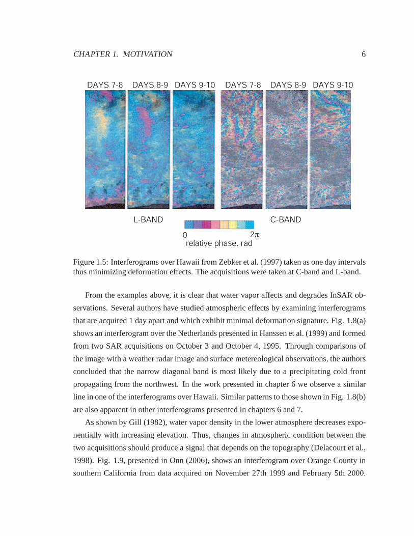
The time series of interferograms presented in Zebker et al.(1997) and reproduced in
Fig. 1.5 shows the atmospheric effect over Hawaii. There is only a one day separation
between the two acquisitions forming the interferogram, therefore we do not expect to see
a significant deformation signature. These interferogramsare formed at both L-band and
C-band. The authors observe from Fig. 1.5 the frequency independence of the unknown
time delay from the tropospheric distortion and hence it cannot be corrected with multi-
frequency analysis. The effect is more pronounced at lower elevations where the path
through the troposphere is longest and more sensitive to variation (Zebker et al., 1997).
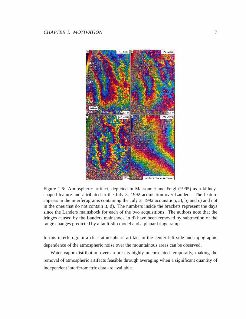
The atmospheric effect in InSAR images has been observed since the first interfero-
grams were created. Massonnet and Feigl (1995) show post-seismic images of Landers’
earthquake with an example of a kidney-shaped atmospheric artifact attributed to the July
3, 1992 acquisition (see Fig. 1.6).
Peltzer et al. (1998) studied post-seismic deformation after the Landers (1992) earth-
quake. The interferogram, see Fig. 1.7(a), has a distinct atmospheric error signature. Addi-
tionally, the line of sight surface displacement profiles plotted by the authors (Fig. 1.7(b) )
show a large irregularity in profiles 2 and 3 between 10 and 20 km east of the fault. The au-
thors attribute the signal to a topographic residual probably caused by an anomalous phase
propagation delay in the image of Sept. 27, 1992, which is common to both profiles. This
example further illustrates the introduction of atmospheric distortions into InSAR images,
caused by atmospheric water vapor, which are comparable in magnitude to the deformation
signatures from crustal motion.
CHAPTER 1. MOTIVATION 6
DAYS 7-8 DAYS 9-10DAYS 8-9 DAYS 7-8 DAYS 9-10DAYS 8-9
C-BANDL-BAND
0 2π
relative phase, rad
Figure 1.5: Interferograms over Hawaii from Zebker et al. (1997) taken as one day intervalsthus minimizing deformation effects. The acquisitions were taken at C-band and L-band.
From the examples above, it is clear that water vapor affectsand degrades InSAR ob-
servations. Several authors have studied atmospheric effects by examining interferograms
that are acquired 1 day apart and which exhibit minimal deformation signature. Fig. 1.8(a)
shows an interferogram over the Netherlands presented in Hanssen et al. (1999) and formed
from two SAR acquisitions on October 3 and October 4, 1995. Through comparisons of
the image with a weather radar image and surface metereological observations, the authors
concluded that the narrow diagonal band is most likely due toa precipitating cold front
propagating from the northwest. In the work presented in chapter 6 we observe a similar
line in one of the interferograms over Hawaii. Similar patterns to those shown in Fig. 1.8(b)
are also apparent in other interferograms presented in chapters 6 and 7.
As shown by Gill (1982), water vapor density in the lower atmosphere decreases expo-
nentially with increasing elevation. Thus, changes in atmospheric condition between the
two acquisitions should produce a signal that depends on thetopography (Delacourt et al.,
1998). Fig. 1.9, presented in Onn (2006), shows an interferogram over Orange County in
southern California from data acquired on November 27th 1999 and February 5th 2000.
CHAPTER 1. MOTIVATION 7
[+5,+180] [+5,+426]
[+5,+40] [-65,+355]
a b
c d48 m53 m
-17 m Landers model removed
5 km
Figure 1.6: Atmospheric artifact, depicted in Massonnet and Feigl (1995) as a kidney-shaped feature and attributed to the July 3, 1992 acquisition over Landers. The featureappears in the interferograms containing the July 3, 1992 acquisition, a), b) and c) and notin the ones that do not contain it, d). The numbers inside the brackets represent the dayssince the Landers mainshock for each of the two acquisitions. The authors note that thefringes caused by the Landers mainshock in d) have been removed by subtraction of therange changes predicted by a fault-slip model and a planar fringe ramp.
In this interferogram a clear atmospheric artifact in the center left side and topographic
dependence of the atmospheric noise over the mountainous areas can be observed.
Water vapor distribution over an area is highly uncorrelated temporally, making the
removal of atmospheric artifacts feasible through averaging when a significant quantity of
independent interferometric data are available.

CHAPTER 1. MOTIVATION 8
34o 30'
-116o 45'34o 00'
-116o 15'
(a) InSAR images over the Landers area.
0
-5
5
0 20 40-20-40
horizontal distance (km)dis
pla
cem
ent to
ward
sate
llite
(cm
)
1
2
3
4
5
6
7
(b) Landers
Figure 1.7: InSAR images over the Landers area.
(a) Cold front images from Hanssen et al. (1999).A. InSAR image from 3 and 4 October 1995 at21:41 UTC. B. Weather radar image of 4 October1995 at 21:45 UTC.
(b) Precipitation images from Hanssen et al.(1999). A. InSAR image from 29 and 30 August1995 at 21:41 UTC. B. Weather radar image of 29August 1995 at 21:45 UTC.
Figure 1.8: Images over the Netherlands showing different weather patterns.
From the examples above it is clear that the increase in temporal density of interfer-
ograms made possible through the use of ScanSAR can greatly improve the accuracy of

CHAPTER 1. MOTIVATION 9
Figure 1.9: Interferogram over Orange County, Los Angeles (Onn, 2006) from SAR acqui-sitions on November 27th 1999 and February 5th 2000 with topographic phase removed.
InSAR observations. High temporal observation density is desirable for both i) studying
rapidly time varying and non-steady geophysical events andfor ii) atmospheric cancella-
tion.
1.2 Objectives
In this work, we present a method to generate stripmap-to-ScanSAR interferograms from
Envisat raw data acquisitions. The primary objectives of this work are to present a method
that allows the easy creation of such interferograms, to demonstrate how using ScanSAR
can increase the density of interferograms during a particular time period and to illustrate
the advantages of higher density in reducing atmospheric noise.
In chapter 2 we review the synthetic aperture radar (SAR) andinterferometric synthetic
aperture radar (InSAR) concepts needed to understand the proposed method and the trade-
offs present. The Envisat radar and its stripmap and ScanSARmodes are described in
chapter 3. The differences between the two modes will be explained in that chapter.

CHAPTER 1. MOTIVATION 10
To generate stripmap-to-ScanSAR interferograms accurately and efficiently it is neces-
sary to process data in these two modes differently than in conventional SAR and InSAR
data reduction, as explained in chapter 4 and chapter 5. The most obvious difference of the
two modes is that ScanSAR data is acquired in so-called burstmode (Cumming and Wong,
2005). In chapter 4 we will describe several methods proposed in the literature for pro-
cessing burst data. For Envisat, the two modes also differ inthe pulse repetition frequency
(PRF), and so in chapter 5 we explain how to overcome this limitation. Additionally, be-
cause of the burst nature of the ScanSAR mode it was necessaryto develop a new method
for co-registering one acquisition to the other. Our approach is described in chapter 5.
We present two interferograms generated using the proposedmethod in chapter 6. We
evaluate the algorithm by selecting two stripmap acquisitions, generating a stripmap-to-
stripmap interferogram, and comparing it to the stripmap-to-ScanSAR interferogram.
Finally in chapter 7 we demonstrate the aforementioned benefits of adding stripmap-
to-ScanSAR interferograms to conventional stripmap interferograms when analyzing geo-
physical events. We show a data series of interferograms composed of both stripmap-to-
stripmap and strimpmap-to-ScanSAR interferograms in chapter 7. In chapter 7 we demon-
strate superior atmospheric compensation by incorporating stripmap to ScanSAR interfer-
ograms to a stack of conventional interferograms.
1.3 Contributions
In this work we have used data from Envisat ASAR instrument togenerate stripmap-to-
ScanSAR interferograms. The specific contributions of thisdissertation are as follows:
(1) A new method for creating stripmap-to-ScanSAR interferograms, including
(a) An algorithm for focusing stripmap and ScanSAR data withdifferent PRFs
(b) Methods for the co-registration and fine registration ofstripmap data to ScanSAR
data.
(c) Relation between burst overlap pixels and chirp-z transform reference function.

CHAPTER 1. MOTIVATION 11
(2) A data series of stripmap-to-stripmap and stripmap-to-ScanSAR interferograms over
Hawaii
(3) A demonstration of atmospheric artifact compensation from stacking stripmap-to-
stripmap and stripmap-to-ScanSAR interferograms.

Chapter 2
InSAR
2.1 Introduction
Our main objective in this research is to develop a practicalmethod to generate stripmap-to-
ScanSAR images, increasing the temporal density of interferometric images. As explained
in chapter 1, finer temporal spacing helps with i) observing rapidly time varying or non-
steady geophysical events and ii) compensating for atmospheric artifacts. In this chapter we
explain the concepts of interferometric synthetic aperture radar (InSAR) needed to motivate
and understand the method proposed in this work, and also thetrade-offs present while
generating such interferograms.
A radar measures the distance between the sensor and objectsbeing observed by trans-
mitting radio frequency signals that reflect from the objects and are subsequently detected
by the sensor. Reflections from multiple objects arrive at the radar at different times, each
depending on the precise range between the object and the sensor (Curlander and Mc-
Donough, 1991). In a typical mapping application, all scattering centers on a surface act
as objects to be observed. Imaging radars produce images of the observed surface, where
the brightness is primarily a function of surface reflectivity and roughness, as well as the
incidence angle.
12

CHAPTER 2. INSAR 13
2.2 SAR
Synthetic Aperture Radar (SAR) is a side-looking imaging radar that achieves fine resolu-
tion in the along-track direction through matched filteringof a set of radar echoes with the
Doppler, or phase, history of a target. Figure 2.1 illustrates the geometry and terminology
describing a SAR acquisition.
v
a
zim
uth
(alo
ng-tr
ack)
ground range(across-track)
swath widthslant range
heig
ht
θ
Figure 2.1: SAR geometry. The SAR flies along-track at velocity v transmitting a series ofRF pulses at the pulse repetition frequency,PRF. The SAR’s image coordinate system isslant range, or distance from the SAR to the ground, and azimuth or along-track direction.The look angle, meassured between the SAR nadir point and theground image points isθ .
The SAR transmits a series of microwave pulses at a rate denoted the pulse repeti-
tion frequency (PRF), as the satellite moves along track with velocityv. The along-track
direction of the radar illumination pattern on the ground isconventionally referred to as
azimuth and the across-track as range (see Fig. 2.1). The SARilluminates the ground at an
across-track angleθ , denoted the look angle.
The transmitted RF pulses scatter off ground objects and theSAR instrument samples
the backscattered radar echos at a rate offs. A swath is the across-track area illuminated

CHAPTER 2. INSAR 14
on the ground with RF pulses, as it moves along track with velocity v. Echoes from objects
within a swath at different slant ranges, that is across-track positions, will arrive at different
times. The radar then records the return signal as a functionof time. For the final image
to represent the ground range direction, a projection from slant range to ground range is
necessary. Each received pulse contains echoes from a full antenna beamwidth of targets
in the azimuth direction.
The resolution of an image can be defined as the minimum distance at which two objects
are distinguishable. Without matched filtering, the slant range (y) resolution, is
δy =c · τ2
(2.1)
wherec is the speed of light, and is proportional to the transmittedpulse width (τ). The
azimuth (x) resolution is proportional to the antenna beamwidth:
δx =rλL
(2.2)
whereL is the antenna length,r is the slant-range distance from the SAR to the imaged area
andλ is the wavelength. For the SAR system used in this work, Envisat ASAR, this results
in range and azimuth resolutions on the order of 5 kilometers, which is unacceptably large
for most geophysical studies.
The signal to noise ratio, SNR, of a resolution cell in a radarimage is the ratio of the
reflected power received at the sensor, to the system noise. The signal power received at
the radar, from the radar equation (Curlander and McDonough, 1991), is:
Pr =PtGt
4πr2 ·c · τ2
·rλL
·σ0 ·Ar
4πr2 (2.3)
wherePt is the transmitted power,Gt is the gain of the transmitter’s antenna,r is the range
distance from the SAR to the resolution cell,σ0 is the normalized radar cross-section and
Ar is the area of the receiving antenna. From the above equations, it is clear that the SNR
depends on the product of the power of the transmitted pulse (Pt) and the pulse length (τ).
We note that given the resolution and SNR relations above, there exists a design tradeoff
dependent on the pulse length. To achieve very fine resolution one needs to transmit very

CHAPTER 2. INSAR 15
short pulses, but high SNR requires either long pulses or impractically very high power.
The use of matched filtering with a chirp pulse avoids this tradeoff by allowing a long
pulse while maintaining fine resolution.
Matched filtering consists of convolving the received signal with the complex conjugate
of the known transmitted signal. Matched filtering is optimal for increasing the SNR in the
least squares sense. Convolving a chirp signal with its conjugate results in a sinc impulse
response if the spectral weighting of the pulse is uniform, resulting in a “compressed”
echo with high SNR at its center. The slant range resolution in this case depends on the
bandwidth (BW ) and not the actual pulse length:
δy =c
2BW(2.4)
Thus, SNR and resolution are decoupled and no longer enforcea tight design tradeoff. A
chirp signal is advantageous because it is a linear-frequency modulated waveform covering
a wide bandwidth and is both easy to generate and to model. Theform of a chirp signal is:
s(tr) = e− j[πKrt2r +2π fctr], for−
τ2
< tr <τ2
(2.5)
whereKr is the chirp slope (Hz/s),fc is the center frequency andtr is the time in the range
direction. From equation 2.5 a chirp signal has a quadratic,in time, phase term, or equiva-
lently a linear frequency dependence on time since the instantaneous angular frequency is
related to the phase through:
f (tr) =1
2πd
dtrφ(tr) (2.6)
The chirp bandwidthBW is expressible as:
BW = Kr · τ (2.7)
Thus properly choosingKr allows for longer pulses with fine resolution.
CHAPTER 2. INSAR 16
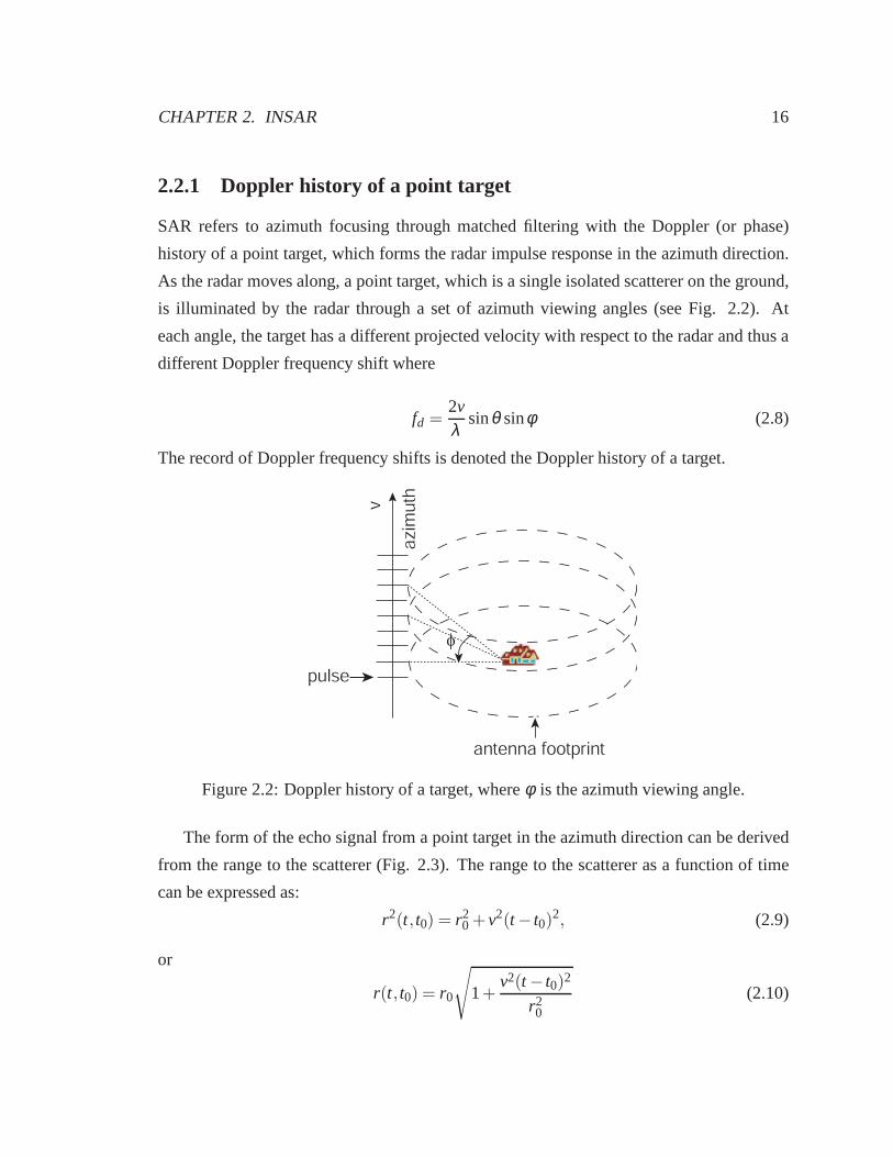
2.2.1 Doppler history of a point target
SAR refers to azimuth focusing through matched filtering with the Doppler (or phase)
history of a point target, which forms the radar impulse response in the azimuth direction.
As the radar moves along, a point target, which is a single isolated scatterer on the ground,
is illuminated by the radar through a set of azimuth viewing angles (see Fig. 2.2). At
each angle, the target has a different projected velocity with respect to the radar and thus a
different Doppler frequency shift where
fd =2vλ
sinθ sinφ (2.8)
The record of Doppler frequency shifts is denoted the Doppler history of a target.
φ
pulse
azi
mu
thv
antenna footprint
Figure 2.2: Doppler history of a target, whereφ is the azimuth viewing angle.
The form of the echo signal from a point target in the azimuth direction can be derived
from the range to the scatterer (Fig. 2.3). The range to the scatterer as a function of time
can be expressed as:
r2(t, t0) = r20 + v2(t − t0)
2, (2.9)
or
r(t, t0) = r0
√
1+v2(t − t0)2
r20
(2.10)

CHAPTER 2. INSAR 17
point scatterer
t
t0v
r0
r0
r(t)
x′
Figure 2.3: Geometry for a single scatterer assuming a straight line radar path and planeearth geometry. We have definedt as the current azimuth time at which the point scattereris imaged,t0 as the time at which the scatterer will be imaged at the centerof the beam,x′ as the distance between the target and the center of the beam and v is the radar velocity.The range to the point scatterer at the current time isr(t) and the range to the point scattererwhen it is a the center of the beam isr0.
Using a first order Taylor series expansion for the range, sincer0 >> v(t − t0):
r(t, t0) ≈ r0(1+v2(t − t0)2
2r20
) = r0+v2(t − t0)2
2r0(2.11)
The phase difference between the transmitted and received waveforms due to the two
way travel to the scatterer will then be:
φ(t, t0) =−4π
λ[r0+
v2(t2−2t0t + t20)
2r0] (2.12)
Thus, omitting the amplitude term, after range processing of any given return, the signal in
azimuth from the single scatterer at locationvt0 with the radar atvt will be:
s(t, t0) = e− j2πv2
λ r0[t2−2t0t+t2
0]e− j4π
λ r0 (2.13)

CHAPTER 2. INSAR 18
To simplify the notation, let the azimuth Doppler ratefR = −2v2
λ r0, so that:
s(t, t0) = e jπ fR[t2−2t0t+t20]e
− j4πλ r0 (2.14)
From equation 2.14 , we can see that the Doppler history of a point target is also a
chirp signal, since it is quadratic in time. Through matchedfiltering fine resolution is then
achieved. The name synthetic aperture radar (SAR) is used because through signal pro-
cessing, i.e. matched filtering, resolution equivalent to alarge aperture antenna is attained.
2.2.2 Typical processing
Fig. 2.4 summarizes the typical processing steps, as discussed thus far, needed to produce
a focused SAR image.
Range CompressionConvolve with range reference function
Azimuth CompressionConvolve with azimuth reference function
raw data
image
Figure 2.4: Typical SAR processing steps.
According to Curlander and McDonough (1991), the resultingSAR azimuth resolution
from matched filtering is:
δx =L2
(2.15)

CHAPTER 2. INSAR 19
The slant range resolution is, from equation 2.4 and equation 2.7,
δy =c
2Krτ(2.16)
whereKr is the chirp signal’s slope andτ is the duration of the chirp signal. In the case
of Envisat’s ASAR instrument the azimuth resolution in the normal SAR mode is 5 meters
and the ground range resolution is approximately 25 m.
Fig. 2.5 shows an example SAR image over Hawaii’s Mauna Kea volcano acquired
from an Envisat pass on November 22, 2004. The ground pixel spacing in the image is
about 30 m. The resulting focused SAR image forms a two-dimensional matrix of pix-
els, with azimuth in the row direction and range in the columndirection. Each pixel is a
complex number with an amplitude and a phase; only the amplitudes are shown in Fig.
2.5. Typically, slight oversampling is used, with a pixel size somewhat smaller than the
resolution size.
azimuth
range2 km
N
Figure 2.5: Amplitude of a SAR image taken from Envisat on November 22,2004 of MaunaKea volcano in Hawaii’s Big Island. The ground pixel spacingin the image is about 30 m.

CHAPTER 2. INSAR 20
Since the resolution size is much greater than a wavelength,there will be many scat-
terers within a resolution cell (resel), the minimum resolvable entity. Each pixel is the
result of the superposition of echos from the scatterers located at a resolution cell centered
on that pixel. The phases of the echos coming from the scatterers within a resolution ele-
ment tend to be uniformly distributed between [0,2π ], thus the resulting pattern (degree of
superposition versus cancellation) will differ across theimage. This causes an amplitude
variation, or graininess, across the image which is denotedas speckle (Goodman, 1984).
The speckle can be reduced by averaging adjacent pixels, in radar this is commonly referred
to as "taking looks".
2.2.3 Doppler centroid
Typically, during a SAR acquisition, the radar antenna doesnot point in a direction perpen-
dicular to the flight direction. The squint angle,φs in Fig. 2.6, is a measure of the angle
deviation from broadside.
Due to lack of control of satellite pointing, the squint angle will often vary among
acquisitions. The squint angle can be determined from the radar echoes due to its relation
(equation 2.17) to the Doppler centroid,fDC:
fDC =2vλ
sinθ sinφs (2.17)
We can estimate the Doppler centroid by i) plotting the average spectrum of Doppler
frequencies and choosing the centroid as the frequency withthe highest amplitude or ii)
using the average incremental phase shift of pixels from azimuth line to azimuth line. Both
methods rely on the Doppler frequency being a function of thetarget’s position in the beam,
see Fig. 2.2 and equation 2.8.
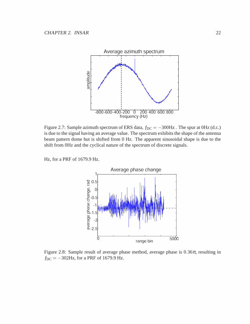
The Doppler spectrum follows the antenna beam pattern, as Fig. 2.7 demonstrates, with
the highest gain at the centroid. In method i) Doppler spectra are incoherently averaged
over several range columns to smooth out the effect of brighttargets in the image and the
frequency with highest amplitude is chosen asfDC. A typical squinted spectrum, with
fDC = −300Hz, is shown in Fig. 2.7.
As Fig. 2.2 demonstrates, a target at a particular range has aslightly different frequency

CHAPTER 2. INSAR 21
v
he
igh
tθ
φs
Figure 2.6: Squinted SAR geometry. A typical SAR does not point in a direction perpen-dicular to the along-track direction but instead there is a squint angle,φs, deviating fromthe perpendicular direction. The target will enter the beamatφsmin or with positive Dopplerfrequency and will leave atφsmax with negative Doppler frequency.
shift for the next pulse because of the slightly different velocity towards the sensor. From
equation 2.6 frequency is proportional to change in phase. In method ii), Madsen (1989)
proposed using an average of the phase increment among adjacent pulses within a range
column to estimate the Doppler centroid (Hanssen, 2001). Averaging helps because the
larger signals, on average, are expected to come from the center of the beam. One full
cycle of phase change corresponds to a Doppler frequency of the PRF. The average phase
is calculated by averaging the complex signal increment andthen finding its angle, to avoid
phase unwrapping problems while averaging phase directly (Cumming and Wong, 2005).
Fig. 2.8 shows a typical result with an average phase of−0.36π which corresponds to -302
CHAPTER 2. INSAR 22
-800-600-400-200 0 200 400 600 800frequency (Hz)
am
plit
ud
e
Average azimuth spectrum
Figure 2.7: Sample azimuth spectrum of ERS data,fDC =−300Hz . The spur at 0Hz (d.c.)is due to the signal having an average value. The spectrum exhibits the shape of the antennabeam pattern dome but is shifted from 0 Hz. The apparent sinusoidal shape is due to theshift from 0Hz and the cyclical nature of the spectrum of discrete signals.
Hz, for a PRF of 1679.9 Hz.
range bin
ave
rag
e p
ha
se c
ha
ng
e,
rad
1
0.5
0
-0.5
-1
-1.5
-2
-2.5
50000
Average phase change
Figure 2.8: Sample result of average phase method, average phase is 0.36π , resulting infDC = −302Hz, for a PRF of 1679.9 Hz.

CHAPTER 2. INSAR 23
2.2.4 Range cell migration
Another important factor in the implementation of SAR processing is range cell migration
(RCM). In SAR the azimuth and range positions of a pixel are coupled, since the range to
a target depends on the azimuth time and follows a curved path(see equation 2.10 and Fig.
2.9). Range cell migration occurs when the curved path spansseveral range columns. Fig.
2.9 demonstrates a typical curved range history. Each of thecolumns bordered by a green
dashed line represents a range cell. In this case, there are three range cells of migration
during the time span shown.
0 5 10 15
-0.4
-0.2
0
0.2
0.4
0.6Range Cell Migration
Range Migration (m)
Azi
mu
th t
ime
(t')
, (s
)
Figure 2.9: A target’s range cell migration curvature with linear and quadratic components.A range cell is represented as a column 4m in width enclosed invertical green dashedlines. During the 1.2 s time span shown, there is a total of three cells of migration. Atypical Envisat full aperture is around 0.6 s.
In a very simple SAR processing algorithm, the azimuth matched filter is applied col-
umn by column, effectively assuming uncoupled directions.To avoid a loss of resolution
while applying the matched filter column by column, the data may be first cut and pasted
to place a given’s target signature entirely within one column. The cut and paste algorithm
is implemented in the azimuth frequency domain where all points at the same range exhibit

CHAPTER 2. INSAR 24
the same curve history. The cut and paste method is not optimal but it is the one often used
because of its computational efficiency since 2D methods areprohibitively inefficient for
processing big radar images.
The amount of range cell migration can be calculated from therange history equation
after power series expansion aroundtDC (Curlander and McDonough, 1991):
r(t ′) = rDC[1−λ fDC
2t ′+
v2
2rDCt′2 + ...] (2.18)
wheret ′ = t − tDC is a new time variable centered attDC, the time the target is imaged at
the center of the beam for squinted geometries, andrDC is the distance from the SAR to the
target attDC.
A migration occurs when the variation in range exceedes a cell size as defined by the
range pixel spacing. From equation 2.18, we note that there is a quadratic term usually
denoted range curvature and a linear term usually denoted range walk. The amount of
range cell migration depends on the integration time and thesquint angle change through
the Doppler centroid.
2.3 Interferometric SAR
Interferometric SAR, or InSAR, consists of a complex combination of two SAR acqui-
sitions. The two acquisitions are separated in time and/or in viewing angles. A small
difference in viewing angles between the two acquisitions typically occurs because the
satellite orbits do not repeat exactly. InSAR imaging geometry is shown in Figure 2.10,
wherei1 and i2 are the incidence angles for each acquisition,r1 and r2 are the distance
from the antenna to the observed object at the Earth surface.The spatial distance between
the two acquisitions is defined as the baseline (B). The parallel component of the baseline
is denotedB‖, while the perpendicular component isB⊥.
We form an interferogram by calculating the complex productof one focused SAR
image with the conjugate of the other focused SAR image. The result is:
s1 · s∗2 = A1A2e jΦ (2.19)

CHAPTER 2. INSAR 25
i2i1
y
z
B
r2
H
∆r,
r1
B
B
Figure 2.10: InSAR geometry. The two satellites shown represent the location of the SARon acquisitions 1 and 2 over the imaged area. A target with height z is at distancesr1 andr2 from the SAR sensor at each of the acquisitions. We have defined B as the baseline,or spatial distance, between the acquisitions,B⊥ as the perpendicular component of thebaseline and i1 and i2 as the incidence angles.
whereΦ is the phase difference between the two SAR image phases andA1 andA2 repre-
sent the amplitudes for each. The scattering phase is similar in both SAR images since they
image the same area, thus most of the phase will cancel out in the phase difference (Zebker
and Villasenor, 1992). The residual phase,Φ, is denoted the interferometric phase and can
be represented as:
Φ = −4πλ
(∆r)+Φnoise (2.20)
where∆r = r2− r1 denotes the path length difference (see Fig. 2.10).
The interferometric phase is in this way a measure of the pathlength difference from the
scatterers to each acquisition location, plus a noise component. The path length difference,
∆r, can be often measured with mm precision. The interferometric phase will be measured
modulo 2π , and each 2π wraparound is typically depicted as a fringe of colors. Fig.2.11
shows an interferogram over Mauna Kea, with a fringe of colors representing 2.8 cm. The

CHAPTER 2. INSAR 26
interferogram was formed with a November 22, 2004 and a January 31, 2005 acquisition.
The measured path length difference in one resolution cell depends on different factors.
It depends on the differences in satellite position and pointing geometry, with a resulting
phaseΦflat. Additionally, it depends on the height of the resolution cell or topography, with
phaseΦtopo. If the two acquisitions are at different times, it also depends on any coherent
movement of the scatterers in between the acquisitions, yielding a phaseΦdefo, and any
differences in the delays as the two signals travel through the variable atmosphere, and
their phase differenceΦatmo. As such, the total interferometric phase can be described as:
Φ = Φflat+Φtopo+Φdefo+Φatmo+Φnoise (2.21)
whereΦnoise is the interferometric phase due to the stochastic component of the phase,
or phase noise, from the many scatterers within a resolutioncell. The non-noise terms
represent coherent contributions from the scatterers.
The desired information for crustal deformation studies isthe change in the path length
with time from surface motion, measured asΦdefo. The interferometric phase signature
expected from a reference ellipsoid assuming no topography, Φflat, can be removed from
the interferogram by using the known look angle and baseline. The resulting interfero-
gram will be dominated by topographic fringes in locations with significant topography.
To subsequently remove the topographic signal,Φtopo, we use a Digital Elevation Map
(DEM) of the area and the perpendicular baseline, with equation 2.22 below to estimate the
topographic signature (Zebker and Goldstein, 1986).
Φtopo = −4πB⊥zλ r sinθ
(2.22)
After these corrections, the deformation phase that arisesfrom movements of the sur-
face in the line of sight direction and the atmospheric phaseremain. The atmospheric phase
can dominate the desired deformation signature. The atmospheric signature is due to de-
lays in the path of the signal as it travels from the radar to Earth and back, encountering
water vapor variability in the troposphere. These delays will be different between the two
acquisitions as the water vapor distribution changes in time. The variability of water va-
por implies that we should stack, or average, several time independent interferograms to

CHAPTER 2. INSAR 27
N
azimuth
range2 km
1 fringe=2π=2.8cm in ∆r
Figure 2.11: InSAR image of Mauna Kea volcano in Hawaii’s BigIsland, formed withacquisitions on November 22, 2004 and on January 31, 2005. The perpendicular baselinebetween acquisitions is about 18 m. The phase is shown superimposed on the amplitude.Each fringe of colors, that is each phase cycle between 0 and 2π , represents 2.8 cm of rangechange. The interferometric phase shown contains the basicfringe pattern, if we assume aflat Earth - decreasing in spatial frequency with range, modulated by topographic features.
decrease the atmospheric artifacts (Zebker et al., 1997).
2.4 Limitations of InSAR
For useful InSAR results the two SAR acquisitions must correlate. Good correlation signi-
fies that the reflected waves from the scatterers that occupy aresolution element (resel) are
similar.
We use the following definition of correlation:
ρ =| < s1s∗2 > |
√
< s1s∗1 >< s2s∗2 >(2.23)
CHAPTER 2. INSAR 28
wheres1 is the signal at the first acquisition,s2 is the signal at the second acquisition and
<> stands for ensemble averaging. Equation 2.23 is the usual correlation definition except
for the absolute value which means that InSAR correlation will vary from 0 to 1.
In InSAR the main sources of decorrelation are:
(1) Thermal decorrelation,ρthermal, which is a function of SNR. It arises from differences
in the noise from using two receivers in the two acquisitions.
(2) Spatial decorrelation,ρspatial, which is a function of the difference in look angles and
thus the perpendicular baseline. Illuminating the same setof scatterers with different
viewing angles results in different range distances to the scatterers within a resolution
element (resel) and thus low correlation (Zebker and Villasenor, 1992). Equation
2.24 below shows the relation between the spatial correlation and the perpendicular
baseline (Zebker and Villasenor, 1992):
ρspatial= 1−2cosθB⊥δy
λ r(2.24)
whereθ is the average of the two incidence angles,B⊥ is the perpendicular baseline,
λ is the wavelength,r is the range distance andδy is the slant range resolution.
(3) Temporal decorrelation,ρtemporal, which is a function of time. If the resolution sur-
face changes between acquisitions the reflected waves from the scatterers will differ.
The total decorrelation is the product of all the decorrelation sources:
ρtotal = ρthermal·ρspatial·ρtemporal (2.25)
To maximize correlation, interferometric pairs should have a small perpendicular base-
line and short time span between the two acquisition times. Other sources of decorrelation,
such as pulse mis-alignment of the two acquisitions, are correctable. In the examples we
will show in chapters 6 and 7 we choose interferometric pairswith perpendicular baselines
below 300 m and with a time span between the pairs below a year.
Moreover for good correlation, there must be significant overlap of the corresponding
azimuth viewing angles during the two acquisitions. For maximum InSAR correlation both

CHAPTER 2. INSAR 29
sets of data need to be processed to the same average Doppler centroid. As will be explained
in chapter 3 ScanSAR illuminates a point target only over a limited number of azimuth
viewing angles making it difficult to overlap ScanSAR pulsesbetween acquisitions. Along-
track timing and control of an orbital SAR at present is inexact, and thus forming ScanSAR
to ScanSAR interferograms is difficult. To ensure sufficientoverlap, the satellite’s azimuth
position at the two acquisitions instances would need to be known precisely and the radar
pulse timing tightly controlled.
2.5 Conclusions
In this chapter, we have presented an overview of InSAR and its limitations introducing
concepts that will be useful for future chapters. InSAR measures path length differences
between acquisitions through the interferometric phase. The desired observable from the
interferometric phase is the deformation signature due to Earth motion. The atmospheric
signature often dominates the desired observable. To suppress the atmospheric signature
several independent interferograms can be stacked. Havinga greater number of such inter-
ferograms in a stack enables measurements of very small surface deformations. ScanSAR
radar operation increases the number of available interferograms. The main objective of
this work is to present a method to produce many stripmap-to-ScanSAR interferograms,
chapters 5 and 6, and to show examples of such interferogramsat a higher density than
is possible with regular stripmap-to-stripmap methods, chapter 7. In the following chap-
ter, we discuss the Envisat SAR instrument, its parameters,and its stripmap and ScanSAR
modes.

Chapter 3
The Envisat satellite
3.1 Introduction
The European Space Agency (ESA) launched the Envisat satellite in March 2002. It is
an advanced polar-orbiting Earth observation satellite which provides measurements of the
atmosphere, ocean, land, and ice. The synthetic aperture radar instrument on Envisat is
denoted Advanced Synthetic Aperture Radar (ASAR). It operates at C-band, with a wave-
length of 5.6 cm.
3.2 Advanced synthetic aperture radar (ASAR)
Currently there are five unclassified Earth remote sensing SAR satellites, ERS-2 and En-
visat from the European Space Agency (ESA), RadarSAT-1 fromthe Canadian Space
Agency and the recently launched ALOS from the Japan Aerospace Exploration Agency
and TerraSAR-X from the German Aerospace Center and EADS Astrium. Envisat repre-
sents the current generation of European Remote Sensing (ERS) satellites following ERS-1
and ERS-2. The ASAR instrument in Envisat uses an active phased-array antenna, capa-
ble of operating at look angles between 15 and 45 degrees. Among other modes, ASAR
includes the traditional stripmap mode and a ScanSAR mode enabled by beam steering in
elevation. The ground coverage afforded by the stripmap andScanSAR operational modes
is illustrated in Fig. 3.1. During ScanSAR mode the satellite electronically steers the beam
30

CHAPTER 3. THE ENVISAT SATELLITE 31
between sub-swaths, while during stripmap mode the beam is maintained within a single
sub-swath. The elevation angle is cycled often enough during ScanSAR operation to per-
mit contiguous ground coverage (see more below). Among the satellites currently in orbit,
RadarSAT-1, Envisat and the recently launched ALOS and TerraSAR-X have ScanSAR
capabilities.
405 km
flight
directi
on
100 km
Figure 3.1: Stripmap acquisition in turquoise versus ScanSAR acquisition in yellow. Dur-ing ScanSAR mode the satellite electronically steers the beam between sub-swaths, whileduring stripmap mode the beam is maintained within a single sub-swath.
3.2.1 ASAR stripmap mode
Stipmap operation is the classic mode for side looking SAR instruments. The instrument
transmits a continuous and periodic sequence of pulses. In this mode, denoted "Image
Mode", or IM, for Envisat, ASAR operates to observe one of seven predetermined swaths.
During stripmap mode a given target is illuminated over a continuous range of azimuth
angles covering the full synthetic aperture,φ ∈ (−β2 , β
2 ), whereβ is the antenna beamwidth
(see Fig. 3.2).
While operating as a stripmap SAR, ASAR is limited to a narrow100 km swath which is

CHAPTER 3. THE ENVISAT SATELLITE 32
v
φβ
Figure 3.2: Ground projected view of a radar viewing a singlepoint scatterer. In stripmapmode the point scatterer is seen by the radar through a continuous set of azimuth viewingangles (φ ). The full antenna beamwidth isβ
imposed by the range ambiguity limitation. The range ambiguity limitation arises because
the radar needs to intersperse transmission and reception of incoming echoes. The echo
from the closest part of the swath must arrive later than the echo from the furthest part of
the swath from the previous pulse.
3.2.2 ASAR ScanSAR mode
We can tradeoff azimuth resolution for wider range coverageusing what is called ScanSAR
mode. If lower resolution, and fewer looks, are acceptable atarget does not need to be
illuminated through the full azimuth aperture. In ScanSAR mode the satellite transmits
a limited sequence of pulses, called a burst, in one sub-swath and then steers the beam
to another sub-swath (see Fig. 3.1). The radar transmits bursts of pulses to each of the
subswaths in turn. After visiting all the sub-swaths, the radar antenna returns to the first
subswath and the scanning cycle repeats. Thus through antenna beam steering the radar
instrument illuminates a wider swath.
In ScanSAR mode a given target is illuminated over a subset ofthe full aperture (φ ∈

CHAPTER 3. THE ENVISAT SATELLITE 33
(−β2 , β
2 )) viewing angles. Each target then has a different Doppler history depending on its
azimuth position with respect to the radar, where the difference corresponds to the along-
track offset of the target.
v
φβ
Figure 3.3: Ground projected view of a radar viewing a singlepoint scatterer. In ScanSARmode the point scatterer is seen by the radar through a discontinuous subset of azimuthviewing angles (φ shadowed).
Burst mode radar was first employed by the Magellan mission tomap Venus’ surface,
in order to reduce data volume and allow the use of other instruments in between radar
bursts (Johnson, 1991) . To our knowledge, the first ScanSAR amplitude image of Earth
is shown in Chang et al. (1996) for the SIR-C satellite and thefirst ScanSAR to ScanSAR
interferogram in Bamler et al. (1999) for the RadarSAT satellite.
The time the radar operates at a particular subswath, creating a burst, must be suffi-
ciently long to produce a continuous image of the ground areaat a desired resolution. The
ScanSAR azimuth (x) resolution for burst by burst processing is related to burst lengthTB
by,
δx =v
BWburst=
vfRTB
, (3.1)
whereBWburst is the azimuth bandwidth of a burst. The resolution does not depend on the
full aperture length, as in stripmap mode, but on the burst size (TB = NB ·TS, whereNB is

CHAPTER 3. THE ENVISAT SATELLITE 34
the number of pulses in a burst andTS = 1/PRF is the sampling period).
By processing all bursts from a particular subswath, a continuous image of the area cov-
ered by that subswath can be synthesised. As illustrated in Fig. 3.4, selecting all the pulses
from a particular ScanSAR subswath results in missing data pulses in between bursts, in
contrast to continuous acquisitions over the subswath during stripmap.
stripmap
scanSAR
NB
NR
Figure 3.4: Azimuth sampling of a particular sub-swath in stripmap and ScanSAR modes.NB is the number of samples in a burst,NR is the burst to burst repetition period in samples.In ScanSAR mode the radar acquires data from other sub-swaths in between the two burstsshown.
In between one set of sub-swath bursts, the radar illuminates other along-track contigu-
ous sub-swaths. Envisat’s ScanSAR mode is denoted "Wide Swath Mode", or WSM, and it
consists of five sub-swaths, for a total imaged swath width inthe range direction of 400 km.
The ScanSAR swath is 400 km rather than 500 km due to the overlaps between adjacent
subswaths. The scanning cycle in ASAR’s ScanSAR mode is sufficiently fast to illuminate
any given target on the ground with three consecutive bursts. From Fig. 3.4 we can ob-
serve another difference between Envisat’s stripmap and ScanSAR mode, that is, the PRF
changes. Because of the PRF difference, pulses within one burst in the ScanSAR image
cannot align identically with stripmap image pulses. In addition, the repeat time between
bursts will generally not be an integer number of pulse periods, thereby complicating the
alignment of the images during interferogram formation. Weaccount for these limitations
in our method, which is presented in chapter 5.

CHAPTER 3. THE ENVISAT SATELLITE 35
Mode Swath NB NR PRF K r τrnge Columns(pulses) (pulses) (Hz) (Hz/s) (µs) (bytes)
Strip IS2 50 317.25 1652.4 5.89e11 27.18 11,612Scan SS1 50 323.28 1684.9 6.98e11 21.14 13,784Strip IS3 65 405.64 2112.6 7.5e11 21.35 11,240Scan SS2 65 403.69 2102.4 7.68e11 16.76 13,784Strip IS4 55 325.46 1695 6.03e11 26.55 13,712Scan SS3 55 325 1692.6 5e11 20.93 13,784Strip IS5 71 399.49 2080.6 7.46e11 21.45 11,276Scan SS4 71 399.49 2080.6 5.66e11 16.87 13,784Strip IS6 60 327.42 1705.2 6.07e11 26.34 13,324Scan SS5 60 327.77 1707 4.24e11 20.72 13,784
Table 3.1: Key Parameters of those ENVISAT/ASAR beams usable for stripmap-to-ScanSAR interferometry. Each stripmap beam has been placednext to its ScanSAR coun-terpart. NB is the number of pulses in one burst andNR is the number of pulses in oneburst to burst repetition cycle.Kr is the chirp slope, whileτrnge is the chirp pulse durationand the chirp bandwidth can be obtained through their multiplication. The range samplingfrequency for all modes and beams is 19.20768 MHz.
The final step in forming a ScanSAR image is to join all of the subswath-processed
images to form the wide swath image. The coverage allowed by awider swath permits
multiple observations of an area within a single orbit cycle, that is, a region of interest is
observed by the sensor on several different orbit tracks. Fig. 1.1 above illustrated the five
Envisat ScanSAR swaths that illuminate Hawaii. For ENVISAT/ASAR therefore, using
ScanSAR, each point on the ground can be imaged five times during a typical 35 day cycle.
3.3 ASAR parameters
ASAR’s most relevant parameters are listed in Table 3.1. Thecorresponding stripmap and
ScanSAR interferometric beams are listed next to each other.

CHAPTER 3. THE ENVISAT SATELLITE 36
3.4 Conclusion
In this chapter we have reviewed the main differences between stripmap and ScanSAR En-
visat modes: continuous data acquisition verses burst-mode data and differences in the PRF
which result in pulse mis-alignments. In chapter 4 and 5 we will show how to overcome
these differences to combine the two modes to create an interferometric image. The values
of the the most important parameters for each of the beams forthe two modes are provided
in table 3.1.
In the following chapters, we present our method to combine stripmap and ScanSAR
acquisitions to form an interferogram and take advantage ofScanSAR’s more frequent
coverage. As explained in chapter 2, to maximize correlation, interferometric pairs should
have a small perpendicular baseline and short time span between the two acquisition times.
Additionally, for maximum InSAR correlation both sets of data need to be processed to the
same average Doppler centroid and any pulse mis-alignment of the two acquisitions needs
to be corrected. Moreover there must be significant overlap of the corresponding azimuth
viewing angles during the two acquisitions. Since ScanSAR illuminates a point target
only over a limited number of azimuth viewing angles, it is difficult to overlap ScanSAR
pulses between acquisitions. Along-track timing and control of an orbital SAR at present
is inexact, and thus forming ScanSAR to ScanSAR interferograms is difficult. To ensure
sufficient overlap, the satellite’s azimuth position at thetwo acquisitions instances would
need to be known precisely and the radar pulse timing tightlycontrolled.
Stripmap-to-ScanSAR interferometric pairs, on the other hand, always overlap, pro-
vided the two Doppler centroids are sufficiently similar to ensure good signal to noise ratio
when both data sets are processed at the same centroid. We canselect the pulses in the
stripmap image corresponding to the available ScanSAR pulses for each ScanSAR burst.
However, since the stripmap image covers a narrower swath than the ScanSAR, stripmap-
to-ScanSAR interferograms observe a given point on the ground less often than would
ScanSAR-to-ScanSAR interferograms, but still more often than stripmap-to-stripmap in-
terferograms. Thus, stripmap-to-ScanSAR interferometric pairs offer a feasible compro-
mise with more frequent coverage than is possible in conventional stripmap-to-stripmap
InSAR. The increase in coverage frequency will be illustrated in chapter 7. In exchange

CHAPTER 3. THE ENVISAT SATELLITE 37
for the increase in frequency of coverage, we must reduce interferogram quality since burst
mode images exhibit lower resolution and fewer looks than stripmap images, as will be
illustrated with interferometric images in chapter 6.

Chapter 4
Azimuth processing of burst-mode SAR
data
4.1 Introduction
In chapter 3 we introduced the main differences between the Envisat stripmap and ScanSAR
modes: continuous data acquisition as opposed to burst-mode data, and also differences in
the PRF which result in pulse mis-alignments. In this chapter we address the former by pre-
senting methods to process burst-mode data. We will discussthe later difference in chapter
5.
Processing stripmap-to-ScanSAR interferometric images differs from conventional stri-
pmap InSAR because of the pulse alignment and sparse sampling issues described in the
previous chapter. Range-Doppler stripmap SAR algorithms,as explained in chapter 2, con-
sist of range compression followed by azimuth compression.Range compression means
matched filtering with the transmitted chirp. Azimuth compression consists of matched fil-
tering with the chirp function from the target’s full aperture Doppler history. As discussed
in chapter 3, ScanSAR data acquisition differs from regularstripmap in the azimuth direc-
tion only. ScanSAR data are acquired in burst mode, limitingthe illumination of a scatterer
in the ground to a subset of the full aperture, and is sampled at a different PRF than stripmap
modes in Envisat. In this chapter, we examine several algorithms presented in the literature
for SAR processing of stripmap and ScanSAR data and describetheir implications for the
38

CHAPTER 4. AZIMUTH PROCESSING OF BURST-MODE SAR DATA 39
method used in this work.
In SAR systems, the impulse response is defined as the system response to a point
target, which is a single isolated scatterer on the ground. Familiarity with this azimuth
response, denoted the Doppler history, as presented in 2.2.1, facilitates the understanding
of the algorithms presented below.
4.2 Algorithms for processing stripmap SAR data
4.2.1 Range-Doppler
A common algorithm for SAR image formation is called range-Doppler; see section 2.2 for
a full description. A block diagram of the range-Doppler algorithm is shown in Fig. 4.1.
Range compression consists of matched filtering with the transmitted chirp signal. Az-
imuth compression is implemented using matched filtering with the the target’s full aper-
ture Doppler history chirp signal, equation 2.14. Both the range compression and azimuth
compression matched filters are often implemented in the frequency domain for computa-
tional efficiency. The required range cell migration correction, or RCMC (see chapter 2),
is applied after the azimuth Fourier transform, denoted here FFT.
4.2.2 Chirp scaling algorithm
The chirp scaling algorithm is an alternative to traditional range-Doppler processing. Chirp
scaling eliminates the inefficient interpolation operation required in range-Doppler during
the range cell migration step. The algorithm is quite accurate over large apertures and mod-
erate squint angles up to 20 degrees for C-band (Davidson et al., 1996) and was introduced
simultaneously in Cumming et al. (1992) and Runge and Bamler(1992), with a thorough
treatment given by Raney et al. (1994). Raney et al. (1994) compare the chirp scaling algo-
rithm to the Range-Doppler algorithm and conclude that the chirp scaling performs better
in terms of range impulse response broadening than the range-Doppler at C-band for squint
angles in the order of 8 degrees or more (see Fig. 4.2). According to Davidson et al. (1996)
for squint angles greater than 20 degrees for C-band and 10 degrees for L-band noticeable

CHAPTER 4. AZIMUTH PROCESSING OF BURST-MODE SAR DATA 40
Raw Data
Azimuth Compression
Azimuth FFT
Range Compression
RCMC
Azimuth IFFT
Compressed Image Data
Figure 4.1: Range-Doppler algorithm block diagram as givenby Cumming and Wong(2005). The range compression and azimuth compression are achieved through matchedfiltering with the transmitted chirp signal and the chirp signal from the Doppler history.RCMC stands for range cell migration correction.
degradations are observed when using chirp scaling due to resolution broadening and an
increase in sidelobe level towards the edges of the range swath.
The range-Doppler algorithm is used frequently because of its favorable tradeoff be-
tween maturity, simplicity, efficiency and accuracy (Cumming and Wong, 2005). However,
the chirp scaling algorithm is advantageous when there is significant range cell migration,
since a large kernel with range-varying coefficients is needed during the range cell migra-
tion correction step in range-Doppler processors.

CHAPTER 4. AZIMUTH PROCESSING OF BURST-MODE SAR DATA 41
azi
mu
th
20 20406080
100120
100120
806040 a
zim
uth
range range20 2040 4060 6080100 100120120 80
Figure 4.2: Contour plots of impulse responses with 8 degreesquint (simulated signals)for the range-Doppler, left, and chirp scaling, right, algorithm after Raney et al. (1994).The range-Doppler algorithm resulting impulse response isclearly broader in the rangedirection than the chirp scaling response.
Additionally, in high squint angle cases, there is a strong cross coupling between range
and azimuth in the range-Doppler algorithm (Cumming and Wong, 2005), requiring a filter
for secondary range compression (Jin, 1984).
As can be seen in the flow chart of Fig. 4.3, the chirp scaling algorithm consists of
FFTs, inverse fourier transforms denoted here IFFTs and complex multiplies by reference
functions. The complex multiplications by complex exponential functions are marked in
Fig. 4.3 with a (*). Raney et al. (1994) include a detailed mathematical analysis of the type
of complex multiplications required. For completeness, the equations have been included
in appendix A.
In the chirp scaling algorithm we first transform the signal in azimuth to the range-
Doppler domain where all targets at a certain range exhibit the same range cell migration
curvature. However, the curvature of targets at different ranges differs (see Fig. 4.4).
To achieve curve equalization a complex multiplication is applied, picking a particular
reference range curvature as the pattern to follow (see appendix A for equations.) The
reference range chosen is arbitrary but typically is the middle of the beam. Once the curves
are equalized a range FFT is applied, followed by a multiplication which implements the
range cell migration correction for the remaining reference curvature and range focusing,
including secondary range compression. Then range IFFT results in a compressed signal
in the range direction with a remaining phase residual. The next steps consist of azimuth
compression and removal of the chirp scaling phase residual.
Both the range-Doppler and the chirp scaling algorithms usethe full azimuth radar
aperture. In ScanSAR, the full aperture is not available, thus we need to employ different

CHAPTER 4. AZIMUTH PROCESSING OF BURST-MODE SAR DATA 42
Raw Data
Reference function(*)
multiply for bulkRCMC,RC and SRC
Compressed Data
Azimuth compression(*)
and phase correction
Range IFFT
Range FFT
Azimuth IFFT
Chirp scaling for(*)
differential RCMC
Azimuth FFT
Figure 4.3: Chirp scaling algorithm block diagram from Cumming and Wong (2005). Chirpscaling is an efficient algorithm for range cell migration compensation. RCMC stands forrange cell migration correction, RC for range compression and SRC for secondary rangecompression.
methods for processing burst-mode data. In the literature,several methods have been pro-
posed to process burst-mode data: traditional full aperture InSAR with zeros in the missing
interburst lines, spectral analysis or SPECAN algorithms,modified SPECAN algorithms,
and extended chirp scaling methods. Here we describe each ofthese methods, in particular
describing in detail the SPECAN and modified SPECAN algorithms from which we derive
our method.

CHAPTER 4. AZIMUTH PROCESSING OF BURST-MODE SAR DATA 43
range
doppler
Rf(f,r1)
Rf(f,rref)
rref
Rf(f,rref) - rref + r1r1
Figure 4.4: Equalized range curvatures resulting from the chirp scaling algorithm fromRaney et al. (1994). The original curves are marked with a dash line, while the equalizedcurves are continuous lines. Note that this figure exaggerates the effect, since in Envisat’scase the differences in the curves is in the order of 10th of meters compared to the rangevalues which are in hundreds of kms.
4.3 Doppler history of a point target in burst mode
The response to a point scatterer on the ground for a burst-mode system can be deduced
from the stripmap response. The response will be that of the Doppler history of a point
target, repeated here from chapter 2,
s(t, t0) = e jπ fR[t2−2t0t+t20]e
− j4πλ r0 (4.1)
multiplied by an impulse train convolved with a burst-sizedrectangle function. From equa-
tion 4.1 the response is then:
s(t, t0)ScanSAR =1
∑n=−1
rect[(t −nTR)
TB]e jπ fR[t2−2t0t+t2
0]e− j4π
λ r0 (4.2)
wheren is the burst number. Here it ranges between -1 and 1 because asnoted in chapter
3 in Envisat ScanSAR a particular target is illuminated in three bursts.TR = NR ·TS is the

CHAPTER 4. AZIMUTH PROCESSING OF BURST-MODE SAR DATA 44
burst repetition interval, andTB = NB ·TS is the burst duration.
4.4 Algorithms for ScanSAR data.
4.4.1 Traditional InSAR with zero padded data
ScanSAR data can be processed using the range Doppler or chirp scaling algorithm after
converting the data to their stripmap equivalent by adding lines of zeros in the interburst
period. This approach to processing, as examined in Bamler and Eineder (1996), preserves
the phase information of the data. However, coherent addition of multiple bursts results
in grating azimuth sidelobes, as we show in Fig. 4.5. From equation 4.2 the impulse
response here for burst mode consists of the full-aperture response multiplied by a burst-
length rectangle function convolved with an impulse train.The response after compression,
Fig. 4.5, is a narrow sinc function, from the full-aperture response, convolved with the
impulse train and multiplied by a wide sinc envelope resulting from the rectangle function
(Bamler and Eineder, 1996).
As suggested in Bamler and Eineder (1996) the modulation artifact can be removed
through low-pass filtering, which extracts the desired envelope. This method suffers from
degraded image quality, that is blurring, due to the modulation artifact. Additionally, it is
inefficient because processing is calculated using the unavailable full aperture. Moreover,
it does not account for the differences in PRF between Envisat’s ScanSAR and stripmap
modes or for the inter-burst period not being an integer multiple of a PRF, all of which lead
to a computationally intensive resampling process. Bamlerand Eineder (1996) account
for non-integer inter-burst period by shifting each burst by an amount between -0.5/PRF
and 0.5/PRF to force an integer inter-burst period, but still the image will not be optimally
focused.
We next present three algorithms, SPECAN, modified SPECAN and extended chirp
scaling, that implement azimuth focusing using only the points sampled during the individ-
ual bursts. The algorithms are thus more efficient.

CHAPTER 4. AZIMUTH PROCESSING OF BURST-MODE SAR DATA 45
azimuth time, t
norm
aliz
ed a
mplit
ude
0
1
0 1/BB-1/BB 2/BB-2/BB
(a) (b)
Figure 4.5: ScanSAR processing by zero padding the inter-burst lines. Images from Bam-ler and Eineder (1996) a) Impulse response.The resulting modulation is evident from thegraph. The desired burst response is the envelope which can be recovered through low passfiltering. b) Image response of a corner reflector.The resulting modulation is evident fromthe multiple lines representing one corner reflector.
4.4.2 The spectral analysis, or SPECAN, method
The SPECAN algorithm was first publicly documented as an alternative to the fast con-
volution algorithm or traditional range-Doppler processor in Sack et al. (1985). However,
the technique and its concepts date back to Caputi (1971); itwas implemented in 1979 at
MacDonald Dettwiler and ESA’s Space Technology Center (ESA-ESTEC) for a real-time
SAR processor.
Consider the equation for the Doppler history of a point target:
s(t, t0) = e jπ fR[t2−2t0t+t20]e
− j4πλ r0 (4.3)
and note that the signal has a quadratic phase term and a linear phase term we should
consider to form the matched filter. To eliminate the quadratic phase term, we multiply the
signal by the complex conjugate of a reference quadratic phase chirp, a step often referred
to as first order de-ramping (Caputi, 1971). If the de-ramping reference term is centered at
boresight (Sack et al., 1985) for an arbitrary location,

CHAPTER 4. AZIMUTH PROCESSING OF BURST-MODE SAR DATA 46
srefderamp(t) = e− jπ fRt2
(4.4)
then the deramped signal is
sderamp(t, t0) = s(t, t0)e− jπ fRt2
= e jπ fR[−2t0t+t20] (4.5)
where we have ignored the azimuth independent propagation delay phase term (e− j4π
λ r0)
and we assume that the radar look direction is perpendicularto the flight path. If this were
not the case, here we would also need to compensate for the average of the stripmap and
ScanSAR data Doppler centroids.
After de-ramping, the linear term remains, along with a constant phase term. That is, we
have a constant frequency sinusoid dependent on azimuth location, and SPECAN employs
FFT methods to estimate the frequency and hence the scatterer position (Caputi, 1971).
However, after the FFT, as will be demonstrated in chapter 5,output sample spacing
varies with the Doppler rate and thus with range, which introduces the need for interpola-
tion, effectively negating any computational advantage from the SPECAN algorithm.
To summarize, SPECAN consists of an azimuth de-ramping function followed by a fast
Fourier transform (FFT), as illustrated in Fig. 4.6. The algorithm requires relatively low
computational rates and is suitable for low resolution imaging. However, when applied
to azimuth processing, the output sample spacing along-track varies with the Doppler rate
and thus with range, which introduces the need for interpolation, effectively negating any
computational advantage. For ScanSAR data, SPECAN processing is done burst by burst
with some zero-padding to the next power of two for FFT efficiency.
4.4.3 Modified SPECAN
In 1998 the modified SPECAN algorithm was introduced by Lanari et al. (1998b), con-
sisting of the same de-ramping function as for SPECAN but with the FFT replaced by a
chirp-z transform (Fig. 4.7).
The chirp-z transform is equivalent to an FFT with an adjustable output bin spacing.
The concept of the chirp-z transform dates back to Rabiner etal. (1969) and the principle

CHAPTER 4. AZIMUTH PROCESSING OF BURST-MODE SAR DATA 47
FFT
sderamp (t)ref
s(t) Interpolate sout (t)
Figure 4.6: Block diagram of SPECAN.
srefderamp(t)
s(t)
sref∗chirp(t) sref∗
chirp(t)
h(t) =srefchirp(t)
out
Figure 4.7: Block diagram of the modified SPECAN.
is shown in Fig. 4.8. The chirp-z transform consists of a multiplication by the conjugate of
a chirp-type reference function, equation 4.6, a convolution by the reference function and
another multiplication by the conjugate of the reference. At the output we obtain samples of
the Fourier transform at a spacing determined by the choice of the chirp reference function.
The chirp reference function has the form:
srefchirp(t) = e j
w0t2
2 (4.6)
wherew0 is an arbitrary variable that the user sets to obtain the desired output sample
spacing.
Lanari et al. (1998b) derive the reference function for range-independent azimuth sam-
ple spacing by assuming an input raw data spatial sampling∆x corresponding to the Nyquist
limit for the stripmap resolution,∆x = L/2. Accordingly, they propose the following refer-
ence function:

CHAPTER 4. AZIMUTH PROCESSING OF BURST-MODE SAR DATA 48
h(t) = schirp
(t)x(t) y(t)
schirp
(t)=ejw0t
2
2
schirp
* (t)ref
ref
ref
schirp
* (t)ref
Figure 4.8: Block diagram of the chirp-z transform.
srefchirp(t) = e jπ rd
r v2t2(4.7)
whererd is a fixed reference range computed from the desired azimuth pixel spacing. Us-
ing this reference function results in sampling spacing that is range independent since the
chosenw0 is inversely proportional to r and the need for interpolation is eliminated. Lanari
verifies that the modified SPECAN algorithm preserves the phase information by using
decimated stripmap raw ERS data to form burst-mode interferograms. But his method as
proposed does not account for possible PRF differences between acquisitions and, more-
over, while he assumes input raw data sample spacing of∆x = L/2, in practice the data are
spaced at∆x = v/PRF. In chapter 5 we will therefore re-derive the requiredsrefchirp(t) for
both stripmap and ScanSAR.
4.4.4 Extended chirp scaling
The extended chirp scaling introduced by Moreira et al. (1996), see Fig. 4.9, is an adap-
tation of the chirp scaling algorithm with shorter azimuth FFTs and IFFTs for burst-mode
data. The extended chirp scaling procedure follows the samesteps as chirp scaling but with
the addition of the SPECAN step at the end, and also with a modification of the azimuth
compression step. During the azimuth compression step, nowcalled azimuth scaling, an
exponential function is introduced that removes the hyperbolic azimuth phase history for
all targets and introduces a constant linear frequency modulation (Moreira et al., 1996). In
this way, the last SPECAN interpolation step is avoided.
The extended chirp scaling algorithm, as with the original chirp scaling counterpart, is
most advantageous when there is significant range cell migration.

CHAPTER 4. AZIMUTH PROCESSING OF BURST-MODE SAR DATA 49
Raw Data
Phase correction andazimuth chirp scaling
Range chirp scalingfor differential RCMC
Azimuth FFTon burst data
Range FFT, phase mu-ltiply, and range IFFT
Azimuth IFFT
SPECAN
Compressed Image Data
Figure 4.9: Extended chirp scaling algorithm block diagramfrom Cumming and Wong(2005)
4.4.5 Our method for processing Envisat data
For burst-mode Envisat data the range cell migration effectis negligible. From equation
2.18 and using Envisat parameters for beam "IS2," the maximum expected curvature mi-
gration is 0.42 bins if we use the full aperture for integration, and only 0.0039 bins if we
use the burst aperture, as is the case during ScanSAR processing. From the processed En-
visat beam "IS2" and "SS1" interferograms in this work, the maximum expected Doppler
centroid is around -139Hz. The maximum expected range walk in these data is 0.155 bins
for full aperture processing or 0.0149 bins for burst by burst processing. The total expected
CHAPTER 4. AZIMUTH PROCESSING OF BURST-MODE SAR DATA 50
range cell migration within a burst is only 0.019 bins, far less than a bin, thus no significant
migration occurs. The extended chirp scaling algorithm advantages thus are not needed
here. We base our method on the modified SPECAN since we can adopt the well tested
range compression part of the range-Doppler algorithm, anduse the de-ramping and chirp-
z transform for the azimuth processing. However, as mentioned above, we will need to
modify the modified SPECAN and re-derive thesrefchirp(t) functions required for processing
stripmap and ScanSAR Envisat raw data.
4.5 Conclusions
In this chapter we reviewed several methods found in the literature for the processing of
burst-mode data. In our work, we begin with the modified SPECAN algorithm because of
its efficiency and ease of use. The modified SPECAN algorithm uses the range processing
steps from the range-Doppler algorithm and the only changesare in the azimuth processing.
The original SPECAN approach is inefficient because of the additional interpolation step,
and the benefits for significant range migration correction of the extended chirp scaling
algorithm are not required for Envisat data.
In the next chapter we present a method for processing stripmap-to-ScanSAR Envisat
interferograms that uses a variation of the modified SPECAN algorithm. The modified
SPECAN algorithm as derived in Lanari et al. (1998b), assuming an input sample spac-
ing of L/2. We then relax this assumption to the natural pulse spacingof v/PRF and we
re-derive the required reference function. Additionally,we suggest using two distinct ref-
erence functions for processing the stripmap and ScanSAR data, respectively, because of
the PRF differences between the two modes in Envisat data.
Chapter 5
Stripmap-to-ScanSAR processing
5.1 Introduction
In chapter 4 we introduced our method to process Envisat ScanSAR data. In this chap-
ter we describe in more detail the azimuth processing steps required to generate stripmap
to ScanSAR interferograms with different PRFs. The azimuthfocusing is based on the
modified SPECAN algorithm that was described in chapter 4, using a modification of the
chirp-z transform reference functions. We start by deriving the needed reference function
for the chirp-z transform step. We then look at an overall block diagram and describe the
processing of both the stripmap and ScanSAR data, delving deeper into the focusing and
co-registration steps.
5.2 Variation of the modified SPECAN
The modified SPECAN as derived in Lanari et al. (1998b) assumes an input sample spacing
of L/2. Here we relax this assumption and use the natural pulse spacing of v/PRF.
We start by discretizing equation 5.1,
sderamp(t, t0) = e jπ fR[−2t0t+t20 ] (5.1)
settingt = kTs−NBTs
2 , wherek is the azimuth sample number, andTs the azimuth sampling
51

CHAPTER 5. STRIPMAP-TO-SCANSAR PROCESSING 52
period, or 1PRF . We sett0 = mTs, that is, the target will bem samples away from the center
of the beam. Following equation 5.1, wheresderampis the azimuth signal after de-ramping,
we obtain the discrete form
sderamp[k,m] = e jπ fR[−2(mTs)(kTs−NBTs
2 )+(mTs)2] (5.2)
Consider the discrete Fourier transform (DFT) ofsderamp, where the DFT of a signal
x[k] is defined as:
DFT(x[k]) =N−1
∑k=0
x[k]e−j 2πkqN (5.3)
Then
DFT(sderamp[k,m])=e jπ fRm(TS)2NBe jπ fR(mTS)2(5.4)
·NB−1
∑k=0
e− j2π fRmT 2S ke
− j 2πkqNB
or, after integration,
DFT(sderamp[k,m])=e jπ fR(mTS)2(NBm +1) (5.5)
·e− j(NB−1) π
NB(q+ fR(mTS)(NBTS))
·NB ·sincNB{2πNB
[q+ fR(mTS)(NBTS)]}
where sincM(w) = 1M
sin(M w2 )
sin( w2 ) is the discrete version of the sinc function,q is the discrete
azimuth frequency variable,NBTS is the length of the burst aperture andTS is 1PRF . Ac-
cording to equation 5.5 each signal peak will be located at bin− fR(mTS)(NBTS). As noted
by Scheiber and Moreira (2000), equation 5.5 further shows that the constant phase offset
depends on the distance from the scatterer to the center of the beam (t0 = mTS).
As noted in chapter 4, the resulting azimuth bin spacing after the DFT varies in the
range direction due to the dependence offR on r0. Thus, the image will be geometrically
distorted. The modified SPECAN algorithm uses the chirp-z transform rather than the DFT
to eliminate ther0 dependence (chapter 4).
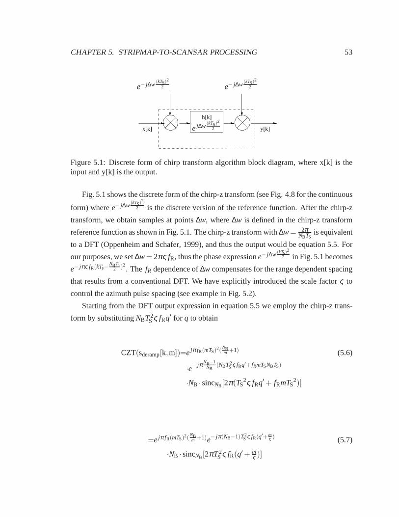
CHAPTER 5. STRIPMAP-TO-SCANSAR PROCESSING 53
x[k]
h[k]
y[k]
e− j∆w(kTS)2
2
e j∆w(kTS)2
2
e− j∆w(kTS)2
2
Figure 5.1: Discrete form of chirp transform algorithm block diagram, where x[k] is theinput and y[k] is the output.
Fig. 5.1 shows the discrete form of the chirp-z transform (see Fig. 4.8 for the continuous
form) wheree− j∆w(kTS)2
2 is the discrete version of the reference function. After thechirp-z
transform, we obtain samples at points∆w, where∆w is defined in the chirp-z transform
reference function as shown in Fig. 5.1. The chirp-z transform with ∆w = 2πNBTS
is equivalent
to a DFT (Oppenheim and Schafer, 1999), and thus the output would be equation 5.5. For
our purposes, we set∆w = 2πς fR, thus the phase expressione− j∆w (kTs)2
2 in Fig. 5.1 becomes
e− jπς fR(kTs−NBTs
2 )2. The fR dependence of∆w compensates for the range dependent spacing
that results from a conventional DFT. We have explicitly introduced the scale factorς to
control the azimuth pulse spacing (see example in Fig. 5.2).
Starting from the DFT output expression in equation 5.5 we employ the chirp-z trans-
form by substitutingNBT 2Sς fRq′ for q to obtain
CZT(sderamp[k,m])=e jπ fR(mTS)2(NBm +1) (5.6)
·e− jπ NB−1
NB(NBT 2
S ς fRq′+ fRmTSNBTS)
·NB ·sincNB[2π(TS2ς fRq′ + fRmTS
2)]
=e jπ fR(mTS)2(NBm +1)e− jπ(NB−1)T 2
S ς fR(q′+ mς ) (5.7)
·NB ·sincNB[2πT 2Sς fR(q′+ m
ς )]

CHAPTER 5. STRIPMAP-TO-SCANSAR PROCESSING 54
-100 -50 0 50 100
Targets centered at +25 and -25, ς=1
Bin number
(a) Settingς to 1
-100 -50 0 50 100
Targets centered at +25 and -25, ς=0.5
Bin number
(b) Settingς to 0.5
Figure 5.2: Changing theς factor in the chirp-z transform reference function affectsoutputsample spacing. The two targets are originally centered at location+25 and−25. After de-ramping and chirp-z transform we obtain the above 1-D impulse responses. As expectedsettingς to 1, left image, results in targets at 25 and−25, while settingς to 0.5, rightimage, results in targets at locations 50 and−50.
Comparison of equation 5.7 with equation 5.5 now shows constant azimuth bin spacing
with range, since the center of the scatterer’s signal, the center of the sinc, no longer de-
pends onfR. Each scatterer’s signal is now centered atq′ = −mς . In addition, through theς
factor the azimuth grid can be chosen as desired.
5.3 Processing steps
In this section we describe the SAR and InSAR processing steps we use to form a stripmap-
to-ScanSAR interferogram. The overall block diagram is illustrated in Fig. 5.3. The blocks
denoted by “(*)” are steps identical to those in a range-Doppler processor. In the follow-
ing sections we will elaborate on the remaining blocks, those that had to be specifically
designed for our method.
We use de-ramping and the chirp-z transform for azimuth processing, after matched
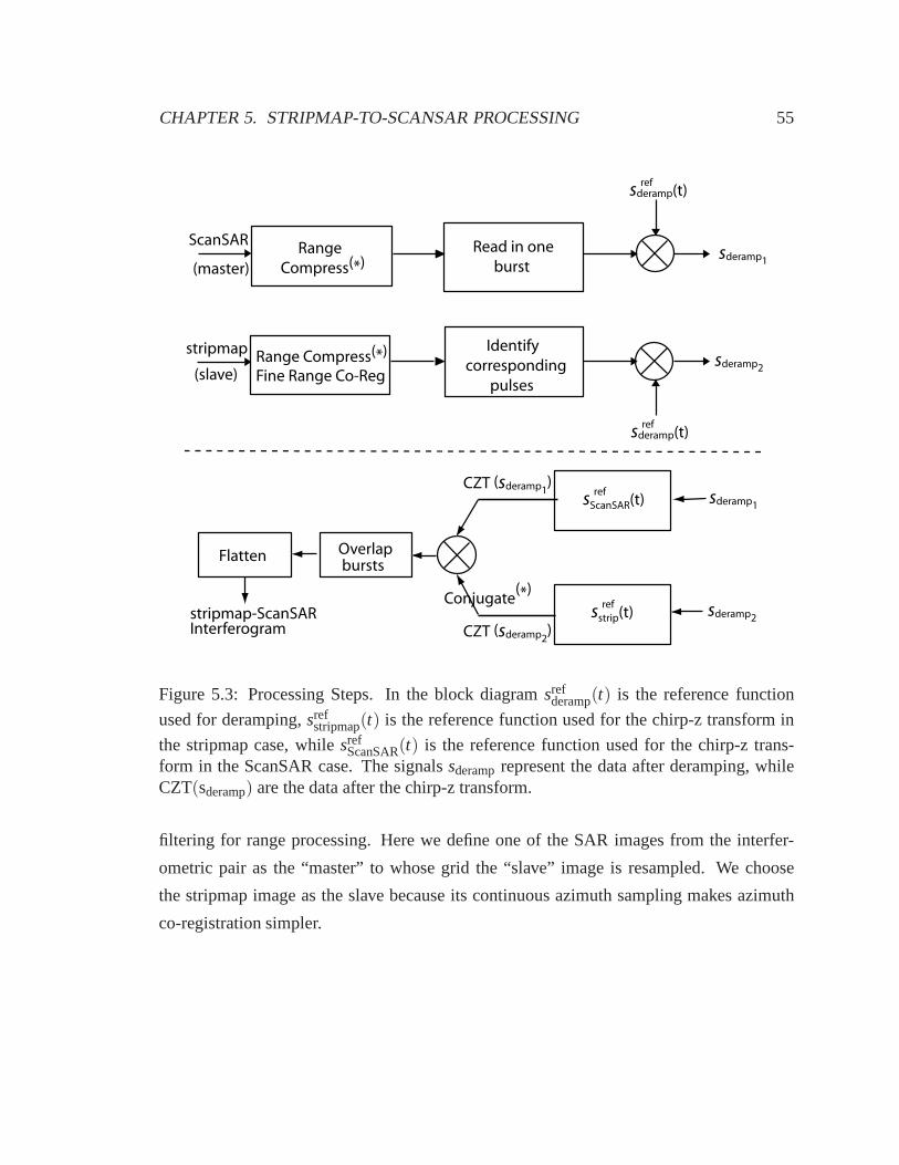
CHAPTER 5. STRIPMAP-TO-SCANSAR PROCESSING 55
ScanSAR
(master)
Range
Compress(*)Read in one
burst
Identify
corresponding
pulses
Range Compress(*)
Fine Range Co-Reg
stripmap
(slave)
sderamp1
sderamp2
sderamp1
sderamp2
sderamp(t)ref
sderamp(t)ref
sScanSAR(t)ref
sstrip(t)ref
CZT (sderamp1)
CZT (sderamp2)
Conjugate(*)
Overlap bursts
Flatten
stripmap-ScanSARInterferogram
Figure 5.3: Processing Steps. In the block diagramsrefderamp(t) is the reference function
used for deramping,srefstripmap(t) is the reference function used for the chirp-z transform in
the stripmap case, whilesrefScanSAR(t) is the reference function used for the chirp-z trans-
form in the ScanSAR case. The signalssderamprepresent the data after deramping, whileCZT(sderamp) are the data after the chirp-z transform.
filtering for range processing. Here we define one of the SAR images from the interfer-
ometric pair as the “master” to whose grid the “slave” image is resampled. We choose
the stripmap image as the slave because its continuous azimuth sampling makes azimuth
co-registration simpler.

CHAPTER 5. STRIPMAP-TO-SCANSAR PROCESSING 56
5.3.1 Co-registering the stripmap image to the ScanSar image
There exists a mis-registration in range and azimuth between the two SAR pairs for InSAR
because of differences in look angle and pulse timing shifts. For good coherence/correlation
we must estimate the mis-registration and co-register the two SARs. In our method to co-
register the two acquisitions in azimuth, we have to determine a coarse azimuth offset as
well as a fine azimuth offset, see Fig. 5.4. We define the coarseazimuth offset as the integer
raw pixel difference of the index of the first azimuth line in the first burst in the ScanSAR
image to its corresponding pulse in the stripmap image. The fine azimuth offset is the sub-
pixel azimuth offset between each corresponding pixel in the two images. The fine azimuth
offset varies in both the range and azimuth directions.
10.5 pixels of azimuth mis-registrationCoarse mis-registrationis 10 pixelsFine mis-registration is 0.5 pixels
Figure 5.4: Azimuth mis-registration
We initially estimate the coarse azimuth offset from the orbital ephemeris and imaging
geometry. Lack of precision of the squint calculation, the angle from antenna pointing
direction to the flight perpendicular, and in the ephemeris parameters limits the accuracy of
this initial estimate.
In common InSAR algorithms the initial estimate of the coarse azimuth offset is refined
by comparing observed features in the master and slave images. The images are usually
processed to the natural azimuth pulse spacing,∆x = vPRF · Re
Re+h , in which we account for
curved orbits and the projection of orbital distances on theground. In the equation for∆x,
Re is the radius of the earth andh is the satellite altitude. In Envisat ASAR ScanSAR, since
the bursts are limited to 50 pulses for ScanSAR beam SS1, the processed image resolution
is about 20 times coarser than for continuous mode imaging, and therefore offset estimates
are that much poorer. One ScanSAR resolution cell (resel), the minimum resolvable entity,
spans approximately twenty five naturally spaced pixels, while in the stripmap case one

CHAPTER 5. STRIPMAP-TO-SCANSAR PROCESSING 57
resel spans approximately one and one half naturally spacedpixels.
We use correlation methods as a next step to refine the initialcoarse offset. Once the
azimuth coarse offset to the stripmap image is determined, we use cumulative pulse timing
information from the stripmap and ScanSAR data to identify burst start indices for the
stripmap data, chosen to match the series of ScanSAR bursts.We account for missing lines
by copying adjacent lines when a line is missing and keeping track of the effect on the
timing. The start indices will not necessarily be integers since the burst-to-burst repetition
interval is not an integer number of pulses, as mentioned in chapter 3. Once the coarse
offsets for each burst are determined, we copy into the computer memory each ScanSAR
burst and the stripmap data corresponding to each ScanSAR burst.
For fine azimuth co-registration, we make use of the phase ramps naturally present
across a burst in ScanSAR mode in incorrectly co-registeredimages (Scheiber and Moreira
(2000) and below, see Fig. 5.8). Correlation methods for thefine-registration of stripmap-
to-stripmap, whose accuracy depends on the resolution cellsize, will not suffice here since
the inherent resolution of the ScanSAR data is 20 times poorer than the stripmap data. For
ERS it has been estimated (Hanssen, 2001) that for sufficiently correlated images, the ac-
curacy of the offsets using incoherent cross-correlation will be about 20 cm in azimuth,
which corresponds to 1/30th of a stripmap azimuth resolution cell. The accuracy of inco-
herent cross-correlations for ScanSAR under these conditions is only 4m, which represents
one raw data pixel ground azimuth distance. Thus, incoherent cross-correlation methods
are sufficient for determining coarse offsets but not fine offsets. The misregistration, if any,
can be inferred much more accurately by estimating the slopeof the azimuth phase-ramps
and is a key part of our method. In the past, a spectral diversity method was used to co-
register ScanSAR-to-ScanSAR images (Scheiber and Moreira, 2000). This method is an
alternative to estimating the phase ramps in each burst.
Our phase ramp algorithm is iterative, where we first assume no misregistration, focus
the images, form the interferogram, and estimate the phase ramp from which we infer the
misregistration present. The process may be repeated to maximize accuracy.
In order to understand the phase ramp, consider the signal from a scatterer viewed
from two acquisitions where one image is mis-registered in azimuth by∆m. The resulting
interferometric phase between the two acquisitions is:

CHAPTER 5. STRIPMAP-TO-SCANSAR PROCESSING 58
Φ = (Φ2−Φ1)+π fRT 2S(∆m+∆m2)+(2π fRT s2∆m)m (5.8)
whereΦ1 andΦ2 are the propagation delay phase terms for acquisition one and two, see
appendix B for a derivation of the equation.
The propagation delay phase term difference (Φ2 −Φ1 = e− j4π
λ ∆r) in equation 5.8 is
the desired deformation interferometric phase difference. The second term represents a
constant in azimuth phase error due to misregistration. Thelast term is a phase error term
that depends on m, that is the target position in azimuth, andthus results in the azimuth
phase ramp. We estimate the misregistration by evaluating the slope inΦ across a burst, and
readjust the output locations for the slave image by the estimated registration error∆m. The
sub-pixel re-sampling is incorporated into the chirp-z transform step for efficiency purposes
(see section 5.3.2). For non-zero Doppler centroids where both images are processed to the
average of the Doppler centroids, equation 5.8 will remain the same except for a constant
phase in the azimuth term (see appendix C.) This does not impact the relation between the
slope and the misregistration.
Range co-registration is done using traditional methods, since in the range direction the
ScanSAR data is similar to the stripmap data. Feature matching for range coarse offset
determination is sufficient. Incoherent cross-correlation methods are adequate, while sub-
optimal, for fine offsets determination in range.
After this step the stripmap image will be co-registered to the ScanSAR image grid. We
next proceed to focus both data sets in the azimuth direction.
5.3.2 Deramping and chirp-z transform
As explained in chapter 4, we use deramping followed by a chirp-z transform to focus the
images in azimuth. The de-ramping reference function is setto:
srefderamp[k] = e− jπ fR(kTS−
NBTS2 )2
(5.9)

CHAPTER 5. STRIPMAP-TO-SCANSAR PROCESSING 59
For the non-zero Doppler centroid case, we can process the images after multiplication
with
srefdop[k] = e− j2π fDCavg(kTS−
NBTS2 ) (5.10)
where fDCavg is the average of the two images’ Doppler centroids. The Doppler centroids
are estimated using the average phase shift from azimuth line to line. We process both sets
of data to the same Doppler to ensure maximal correlation.
Referring to the result after the chirp-z transform, equation 5.7, we can control the
resulting azimuth grid through the constantς . The natural time spacing,TS = 1PRF , equiva-
lent to a distance spacing ofvPRF , follows when the constant,ς , is set to 1. A typical single
look image has a distance azimuth pixel spacing ofvPRF · Re
Re+hm, accounting for the ground
projection. To match, the constant,ς , should be set to 1· Re+hRe
.
For the ScanSAR mode we have a limited number of pulses per burst which results
in rather coarse azimuth resolution. The size of a resel compared to a pixel implies that
resolving each burst to the natural bin spacing will not focus the targets in azimuth to a
single point, but to a sinc-weighted “short line”, Fig. 5.5(a). Thus, for ScanSAR we reduce
oversampling by using a larger pulse spacing. Covering the entire real antenna aperture
width with each burst means that we will see a single scatterer in the maximum number of
consecutive bursts possible, Fig. 5.5(c). Each burst will have an independent look at the
scatterer and the pixels containing the scatterer can then be averaged across the bursts to
reduce speckle. To cover the whole beam width within one burst, we set the constant,ς , toλ r
LNB· PRF
v .
We have already pointed out that Envisat ASAR ScanSAR imageshave differentPRFs
than their stripmap counterparts. Using different reference functions at the chirp-z trans-
form step, as shown in Fig. 5.3, we set the spacing in the ScanSAR image grid to that of the
stripmap image. We thus use differentς constants in the ScanSAR and stripmap reference
functions, differing by a ratio ofPRFstripmapPRFScanSAR
.
The chirp-z transform reference functions used are then:
srefstripmap[k] = e− jπς fR(kTs−
NBTs2 )2
(5.11)
srefScanSAR[k] = e
− jπς ·PRFstripmapPRFScanSAR
· fR(kTs−NBTs
2 )2
(5.12)

CHAPTER 5. STRIPMAP-TO-SCANSAR PROCESSING 60
Image
space
NB
NR
Raw data
space
(a) Natural pulse Spacing (ς = 1 · ReRe+h )
Image
space
NB
NR
Raw data
space
(b) Pulse spacing without overlap between bursts (ς = NRNB
· ReRe+h )
NB
NR
Raw data
space
Image
space
(c) Pulse spacing to cover antenna beamwidth within one burst (ς = λ rLNB
· PRFv )
Figure 5.5: Differentς values amount to different azimuth pulse spacings. On the leftSAR amplitude images for eachς choice. On the right, cartoon showing how theς valueaffects the amount of aperture we see within a burst. In the cartoon images, the scatterer hasbeen blown up to represent the lower resolution of ScanSAR images. Subfigure (a) showsthe “short lines” that result when the pulses are processed to the natural pulse spacing.Subfigure (b) shows the same targets processed to have zero overlap among consecutivebursts. Subfigure (c) shows the targets processed to see a full antenna beamwidth withinone bursts. With this option, the same target will be seen in the maximum number ofconsecutive bursts.
Here as in Lanari et al. (1998b), we implement the convolution part of the chirp-z
transform in the frequency domain. The final block diagram for azimuth focusing is shown

CHAPTER 5. STRIPMAP-TO-SCANSAR PROCESSING 61
in Fig. 5.6. Notice that in the figure we have included the required azimuth shift for co-
registration. As was mentioned in Section 5.3.1, the required fine co-registration can be
incorporated into the deramping and chirp-z transform steps. To account for the shifts,
srefderamp and sref
Stripmap during its first multiplication step, need to have their azimuth time
variable shifted. Additionally, the signal in the frequency domain, after FFT, needs to be
phase shifted (multiplied byej2π k0q
Nf , wherek0 is the shift amount,q is the discrete frequency
variable andNf is the FFT size).
sdop
[k]refs
deramp[k]ref s
ScanSAR [k]ref
FFT
FFT
FFT
FFT
IFFT
IFFT
sScanSAR
[k]ref
sScanSAR
[k]ref*
sdop
[k-k0] s
deramp[k-k
0] s
stripmap [k-k
0]
sstripmap
[k]
sstripmap
[k]
refrefref
ref*
ref
CZT(sderamp1)
CZT(sderamp2)
ej2πk
0[q/Nf-0.5]
Figure 5.6: Azimuth compression and co-registration usingde-ramping and chirp-z trans-form. In the block diagramsref
deramp[k] is the reference function used for deramping,
srefstripmap[k] is the reference function used for the chirp-z transform in the stripmap case,
while srefScanSAR[k] is the reference function used for the chirp-z transform in the ScanSAR
case. The signals CZT(sderamp) are the data after the chirp-z transform. The shift requiredto co-register the stripmap to the ScanSAR grid isk0, while Nf represents the FFT size.
For the stripmap and ScanSAR images, respectively, theς value insref can be adjusted
to set a certain number of overlap pixels between bursts, while maintaining theς ratio
among the two. Overlap pixels are those pixels that show the same scene in neighbor-
ing bursts. Choosing an integer number of overlap pixels simplifies the contiguous bursts

CHAPTER 5. STRIPMAP-TO-SCANSAR PROCESSING 62
overlap step in Fig. 5.3, by avoiding sub-pixel interpolation.
We derive the relation between overlap pixels and the constant ς using the geometry
shown in Fig. 5.7. The figure shows the projected area seen by two successive bursts. The
burst centers are marked with an X. From one burst to the next the radar will have traveled
by a ground projected distance of∆L = NRvPRF · Re
Re+h . The distance between the center of the
burst and both burst edges isNB∆x2 , where∆x is the pulse spacing, controlled throughς .
x
x
Radar Ground
1st Burst Center
2nd Burst Center
0�
NRvPRF · Re
Re+h −NB∆x
2�
NB∆x2NRv
PRF · ReRe+h
∆x = ς ·vPRF
Figure 5.7: Overlap relation between two adjacent bursts. The X mark the center of thebursts and the diagonal lines show the amount of ground area covered by each burst.
Defining the number of overlap pixels asopixels, we obtain:
opixels·∆x =NB∆x
2− [
NRvPRF
·Re
Re+h−
NB∆x2
] (5.13)
where∆x is ς ·vPRF , which simplifies to:
opixels= NB −NR
ς·
Re
Re+h. (5.14)
As an example, to maintain zero pixel overlap between burststhe ς constant is set toNRNB
· ReRe+h (see Fig. 5.5(b)).

CHAPTER 5. STRIPMAP-TO-SCANSAR PROCESSING 63
5.3.3 Azimuth ramps
In equation 5.8 we saw that there is a linear relation betweenthe phase ramp and the amount
of misregistration. As an example, in one Envisat ASAR IM beam IS2 data set we analyzed
here, the main parameters werePRF = 1Ts
= 1652.42, v = 7555.39, λ = 0.056237 and
r0 = 824930.5. The expected slope (from equation 5.8) of the phase ramp is0.00566 per
azimuth pulse or per vPRF for a one pixel offset error. Thus, for a one pixel misregistration
offset, assumingς is set to 6 and 50 pulses per burst, we expect 1.7 radian of phase ramp
per burst. Simulations in which we purposely mis-register the bursts by one pixel in fact
show a 1.7 radian phase ramp. Asr0 changes in the range direction the slope changes
slightly. See Fig. 5.8 for examples of phase ramps when we purposely mis-register the data
by +/-2 raw pulses. As expected, in Fig. 5.8 the sign of the phase ramp is opposite if we
mis-register by +2 (blue to red to yellow) verses -2 (blue to yellow to red) and we get a
total phase ramp across a burst of about 2π radians.
on
e b
urs
to
ne
bu
rst
Figure 5.8: Azimuth phase ramps due to mis-registration. Inthe top image the two SARsare mis-registered by +2 pixels and in the bottom one by -2. Asexpected, the phase rampsin the two images have opposite slopes (blue to red to yellow verses blue to yellow to red)and there is about 2π radians across a burst.

CHAPTER 5. STRIPMAP-TO-SCANSAR PROCESSING 64
We use this linear relation between the phase ramp and the amount of misregistration
to infer the misregistration. Initially we process the images assuming no misregistration.
After the images have been focused we estimate the phase ramp, and then infer the misreg-
istration amount. The calculated misregistration is then used to co-register the images with
sub-pixel accuracy. Once a few bursts are aligned, subsequent bursts are aligned by de-
termining the required co-registration through keeping track of the ScanSAR and stripmap
timing and accounting for missing lines.
5.4 Conclusions
In this chapter we have proposed a method for the full SAR processing of ScanSAR data
and its stripmap pair. The main additions are in the azimuth focusing and co-registration.
For the azimuth focusing, we have used the modified SPECAN with a variation in the
chirp-z transform reference function and used different reference functions for each of the
modes. For the azimuth co-registration, we use correlationfor the coarse co-registration
and estimation of the azimuth ramps for the fine co-registration. In chapter 6 we will
test the method in two stripmap to ScanSAR interferograms and a proof of concept will be
done by comparing a stripmap to stripmap interferogram to the same stripmap to decimated
stripmap which simulates ScanSAR data.

Chapter 6
Two case studies
6.1 Introduction
In chapter 5 we presented our method for processing stripmap-to-ScanSAR interferograms.
In this chapter we apply the method to form two interferograms. Additionally, we evalu-
ate the accuracy of the method by comparing a stripmap-to-stripmap interferogram to a
stripmap-to-ScanSAR interferogram formed with the two same acquisitions but decimat-
ing one to simulate ScanSAR raw data.
6.2 Two case studies
We show here Envisat ASAR beam IS2 and SS1 acquisitions processed to stripmap-ScanSAR
interferograms of the island of Hawaii. The topographic signature is removed in Figs. 6.2
and 6.3. The topographic map in Fig. 6.1 serves as as a reference to locate Mauna Loa
(bottom), Mauna Kea (top) and Kilauea on the bottom right side of the images.
The temporal baseline for the data shown in Fig. 6.2 is 106 days from May 2004 to
September 2004, while for Fig. 6.3 it is 36 days from May 2005 to June 2005. The per-
pendicular baselines are 74 m and 89 m respectively. The phase noise, measured as the
standard deviation of the phase in a high correlation area, in Fig. 6.2 is 0.34 radians and
in Fig. 6.3 is 0.33 radians. Each fringe of colors representsa change in slant range of 2.8
cm. Note the significant atmospheric signature present, which provides further motivation
65

CHAPTER 6. TWO CASE STUDIES 66
Figure 6.1: Reference topographic map.
to process more stripmap-ScanSAR interferograms over Hawaii in order to obtain a denser
time series to help with the atmospheric compensation.
6.3 Proof of concept
In order to verify that the chirp-z transform algorithm presented here preserves the phase
signature of the interferogram we take two stripmap images and convert one of them to a
ScanSAR format by deleting pulses to form bursts. We then form the interferogram and
compare it to its equivalent stripmap-to-stripmap interferogram. Previous such analyses,
using the chirp-z transform, were done with ERS data, as reported by Lanari et al. (1998a).
They used values for the number of pulses in one ScanSAR burstand the repetition interval
among bursts that result in better innate resolution and higher SNR than present in Envisat
ASAR’s ScanSAR to stripmap mode.
Here we do the comparison using Envisat ASAR data and a repetition interval among

CHAPTER 6. TWO CASE STUDIES 67
Mauna Kea
Mauna LoaKilauea
(a) Amplitude and Phase
Mauna Kea
Mauna Loa Kilauea
(b) Phase Only
Figure 6.2: Stripmap-to-ScanSAR inteferogram of the island of Hawaii, 2004/9/13 to2004/5/31B⊥ = 74m
Mauna Kea
Mauna LoaKilauea
(a) Amplitude and Phase
Mauna Kea
KilaueaMauna Loa
(b) Phase
Figure 6.3: Stripmap-to-ScanSAR inteferogram of the island of Hawaii, 2005/05/16 to2005/6/20B⊥ = −89 m.
bursts that results in similar resolution and SNR to that present in Envisat ASAR ScanSAR
to stripmap mode interferograms. These previous comparisons attested to the ability of de-
ramping followed by chirp-z transform to preserve phase integrity, a property we expect to
remain the same when using the actual Envisat ASAR parameters. In this case, we expect

CHAPTER 6. TWO CASE STUDIES 68
to have poorer, but more realistic, phase noise/correlation performance than seen in the
previous comparisons.
For example, Lanari et al. (1998a) used simulated ERS data over Mount Etna with a
resolution of∼ 37 m and 4 azimuth looks, that is, the same scatterer appearedin 4 bursts,
by assuming 128 pulses per burst and repetition interval of 236 pulses. In our verification
we compare a stripmap-to-ScanSAR interferogram, created by decimating the master im-
age to form the ScanSAR part, to its equivalent stripmap-to-stripmap interferogram, using
parameters close to Envisat ASAR SS1 ScanSAR mode. Envisat ASAR ScanSAR SS1
uses 50 pulses in each burst and a repetition interval close to 350 pulses (the actual value
for Envisat ScanSAR is 317.28), giving∼ 102 m resolution and 3 looks.
Comparing the stripmap-to-ScanSAR interferogram in Fig. 6.4 to the stripmap-to-strip-
map interferogram in Fig. 6.5, we see that the phase integrity is preserved since the basic
phase signature is maintained. As expected there is a decrease in the correlation of the
image, with more granularity present in the phase shown in Fig. 6.4, which in many cases
is an acceptable trade off for the increase in time density available in stripmap-to-ScanSAR
interferograms. This can be more readily observed in the correlation images shown in
Fig. 6.7. Note that around Mauna Loa the stripmap-to-stripmap image, Fig. 6.7(b), exhibits
more yellow, representing a higher degree of correlation, than the stripmap-to-ScanSAR
(Fig. 6.7(a)). The correlation in the low correlation partsof the image, such as the ocean,
appears higher than it is in the stripmap-to-ScanSAR Fig. 6.7(a) due to the bias caused by
the loss of looks (Zebker and Chen, 2005).
Another equivalent measure for the decrease in quality is the phase noise in both im-
ages. The rms phase noise of the stripmap-to-ScanSAR interferogram in a high corre-
lation region is 0.181 radians, compared to 0.115 in the sameregion for the stripmap-
to-stripmap, or a decrease in performance ratio of 1.57. This difference is close to the
expected value since the stripmap-to-stripmap image has 11azimuth looks, while the
stripmap-to-ScanSAR has only 4 and thus we expect the phase noise ratio to be around
1.66 (√
114 = 1.66) (Zebker and Villasenor, 1992). We note in passing that the atmospheric
signature in the interferograms in Figs. 6.4 and 6.5 has an interesting shape, tracing a line
of constant elevation around Mauna Loa. The diagonal line found in the center of Figs. 6.4
and 6.5 is similar to the diagonal line found in Hanssen et al.(1999) interferogram over the

CHAPTER 6. TWO CASE STUDIES 69
Mauna LoaKilauea
Mauna Kea
(a) Amplitude and Phase
Mauna Kea
Mauna LoaKilauea
(b) Phase
Figure 6.4: Stripmap-to-ScanSAR Envisat ASAR inteferogram of the island of Hawaiiusing decimated stripmap data as ScanSAR, 2003/12/8 to 2004/2/16B⊥ = 16 m.
Mauna Kea
Mauna LoaKilauea
(a) Amplitude and Phase
Mauna LoaKilauea
Mauna Kea
(b) Phase
Figure 6.5: Stripmap-to-stripmap Envisat ASAR inteferogram of the island of Hawaii,2003/12/8 to 2004/2/16B⊥ = 16 m

CHAPTER 6. TWO CASE STUDIES 70
−π π
Figure 6.6: Difference between the interferograms in Fig. 6.4 and 6.5. A phase constantoffset and a phase ramp in range and azimuth across the entireimage were removed from6.4 before computing the difference.
(a) Coherence for the stripmap-to-ScanSAR (b) Coherence for the stripmap-to-stripmap
0 1
Figure 6.7: Correlation images of the island of Hawaii, 2003/12/8 to 2004/2/16B⊥ = 16m.
Netherlands. Hanssen et al. (1999) attribute the diagonal line to a precipitating cold front.
Propagating clouds could certainly exhibit the quick change in phase delay represented by
the diagonal line.

CHAPTER 6. TWO CASE STUDIES 71
6.4 Conclusions
In this chapter, we have shown that an azimuth SAR processor such as the one described in
chapter 5 permits generation of actual Envisat ASAR stripmap-ScanSAR interferograms.
Our method allows for re-use of many of the tools already available for range-Doppler SAR
processing since the only change is in the azimuth processing.
We have shown here several stripmap-to-ScanSAR interferograms over Hawaii pro-
cessed using the method in chapter 5. We have briefly discussed the method’s performance
by comparing a stripmap-to-stripmap interferogram to its equivalent stripmap-to-simulated
ScanSAR interferogram.
The stripmap-to-ScanSAR interferograms shown in this chapter faithfully reflect the
phase of conventional interferograms, but exhibit fewer looks and coarser resolution com-
pared to their stripmap-to-stripmap counterparts. For many applications, a denser time
series is of foremost importance, and the advantages from the denser time series analy-
sis and temporal averaging possible through stripmap-ScanSAR interferograms offset any
loss in correlation. In chapter 7 we will present a time series of stripmap-to-stripmap and
stripmap-to-ScanSAR interferograms.

Chapter 7
Data series of interferograms
7.1 Introduction
In chapter 5 we presented a method for processing an Envisat ScanSAR-stripmap data
acquisition pair to produce an interferogram. In chapter 6 we tested the method and verified
that it is phase preserving and that there is the expected loss of correlation and available
looks as compared to conventional InSAR. This loss of both correlation and availability of
looks is offset by the possibility of more frequent coveragein time. Here we show a time
series of interferograms with a temporal density that wouldnot be possible if processing
is limited to stripmap-to-stripmap combinations. Additionally, we combine stripmap-to-
stripmap and stripmap-to-ScanSAR interferograms in stacks, or averages, for atmospheric
artifact compensation.
7.2 Selection of interferometric pairs
As remarked in chapter 2, interferometric pairs should be selected to have a small perpen-
dicular baseline (B⊥) to maximize spatial correlation. Additionally, to maximize temporal
correlation, the pair should cover a short time span. We thusconsider both the perpendic-
ular baseline and the time span to select the set of acquisitions to yield the highest quality
interferometric pairs. Typically, a perpendicular baseline below 300m yields high spatial
correlation for C-band interferometry. The timespan necessary for high correlation varies
72

CHAPTER 7. DATA SERIES OF INTERFEROGRAMS 73
depending on the amount of vegetation present in the imaged area. Here we limit the time
span to two years.
In Fig. 7.1 and Fig. 7.2 we plot the perpendicular baseline and time span for each
of our acquistion candidates that image the island of Hawaiifrom Envisat track 200 and
track 429 respectively. The blue dots represent ScanSAR acquisitions while the magenta
dots are stripmap acquisitions. The y-axis portrays the perpendicular baseline, while the
x-axis represents time and each horizontal line is a candidate interferometric pair. The red
horizontal lines join stripmap and ScanSAR pairs while the cyan lines join stripmap and
stripmap pairs. For example, from the graph in Fig. 7.1, the candidate interferometric pair
formed by acquisitions on September 13, 2004 and on January 6, 2005 has a perpendicular
baseline of 45 m.
From the interferometric candidates from track 200, we choose three stripmap-to-strip-
map pairs, marked with a yellow arrow in Fig. 7.1, and three stripmap-to-ScanSAR pairs
marked with a green arrow in Fig. 7.1.
From the interferometric candidates from track 429, we choose four stripmap-to-stripm-
ap pairs, marked with a yellow arrow in Fig. 7.2, and two stripmap-to-ScanSAR pairs
marked with a green arrow in Fig. 7.2. Note that here we only choose two stripmap-to-
ScanSAR pairs because of the lack of availability of pairs with low perpendicular baseline.
Since stripmap-to-ScanSAR pairs already suffer from lowercorrelation, minimizing the
loss of further correlation is beneficial. We processed these the interferometric images and
the results are presented in the following section.
7.3 Data series
Using ScanSAR for generating a series of interferograms is advantageous because there are
more interferograms available in a particular time frame ascompared to using stripmap-
only InSAR. We now present a time series of images of some of Hawaii’s volcanoes using
stripmap-to-ScanSAR and stripmap-to-stripmap interferograms from Envisat tracks 200
and 429.
From Fig. 7.1, we choose highly correlated interferometricpairs from track 200 with
low B⊥ and a small time span. We present three stripmap-to-stripmap interferograms in

CHAPTER 7. DATA SERIES OF INTERFEROGRAMS 74
Sep13Nov12
Jan11Mar12
May11Jul10
Sep8Nov7
Jan60
50
100
150
200
250
300
Interferometric pair candidatesorbit 200
2004 2005
Dates
Pe
rpe
nd
icu
lar
Ba
selin
e
Figure 7.1: Interferometric pair candidates that image theisland of Hawaii in track 200 withB⊥ < 300 m and a time span less than 2 years. Each column of blue dotsis one stripmapacquisition for a particular date, while each column of magenta dots is one ScanSAR ac-quisition for a different date. Each red line represents a stripmap-to-ScanSAR pair, whileeach blue line is a stripmap-to-stripmap pair. The y-axis represents the perpendicular base-line, B⊥, in m, while the x-axis represents dates. The length of each line is a measure ofthe time span between acquisitions in an interferometric pair. The yellow arrows mark thethree stripmap-to-stripmap interferometric pairs presented below, while the green arrowsmark the three stripmap-to-ScanSAR interferometric pairspresented below.
Fig. 7.3 and three stripmap-to-ScanSAR interferograms in Fig. 7.4, Fig. 7.5 and Fig.
7.6. The left-hand side image from the stripmap-to-ScanSARfigures presents the phase
signature modulated by the amplitude for orientation purposes, while the right-hand side
image displays only the phase to make phase accuracy more evident.
From Fig. 7.2, we choose highly correlated interferometricpairs from track 429 with
low B⊥ and small time span. We present four stripmap-to-stripmap interferograms in Fig.
7.7 and two stripmap-to-ScanSAR interferograms in Fig. 7.8and Fig. 7.9.
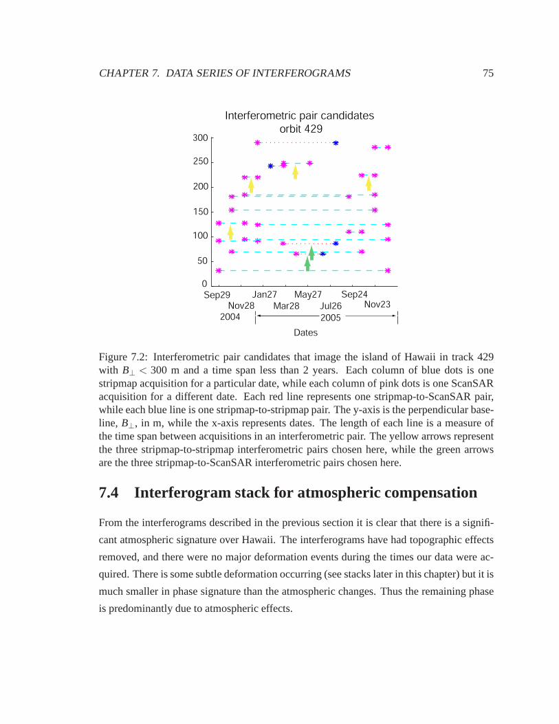
CHAPTER 7. DATA SERIES OF INTERFEROGRAMS 75
0
50
100
150
200
250
300
Interferometric pair candidates orbit 429
Sep29Nov28
Jan27Mar28
May27Jul26
Sep24Nov23
2004 2005
Dates
Figure 7.2: Interferometric pair candidates that image theisland of Hawaii in track 429with B⊥ < 300 m and a time span less than 2 years. Each column of blue dotsis onestripmap acquisition for a particular date, while each column of pink dots is one ScanSARacquisition for a different date. Each red line represents one stripmap-to-ScanSAR pair,while each blue line is one stripmap-to-stripmap pair. The y-axis is the perpendicular base-line, B⊥, in m, while the x-axis represents dates. The length of each line is a measure ofthe time span between acquisitions in an interferometric pair. The yellow arrows representthe three stripmap-to-stripmap interferometric pairs chosen here, while the green arrowsare the three stripmap-to-ScanSAR interferometric pairs chosen here.
7.4 Interferogram stack for atmospheric compensation
From the interferograms described in the previous section it is clear that there is a signifi-
cant atmospheric signature over Hawaii. The interferograms have had topographic effects
removed, and there were no major deformation events during the times our data were ac-
quired. There is some subtle deformation occurring (see stacks later in this chapter) but it is
much smaller in phase signature than the atmospheric changes. Thus the remaining phase
is predominantly due to atmospheric effects.

CHAPTER 7. DATA SERIES OF INTERFEROGRAMS 76
(a) InSAR image formed with acquisitions onNovember 22, 2004 and on December 27, 2004.The perpendicular baseline between acquisitions isabout 76 m and the parallel baseline is about 25 m.The phase noise is 0.139.
(b) InSAR image formed with acquisitions onDecember 27, 2004 and on January 31, 2005.The perpendicular baseline between acquisitions isabout 51 m and the parallel baseline is about 6 m.The phase noise is 0.168.
(c) InSAR image formed with acquisitions on Jan-uary 31, 2005 and on March 7, 2005. The perpen-dicular baseline between acquisitions is about 27 mand the parallel baseline is about 32 m. The phasenoise is 0.109.
Figure 7.3: Stripmap-to-stripmap InSAR images of the island of Hawaii. The phase isshown superimposed on the amplitude. Each fringe of colors,that is each phase cycle be-tween 0 and 2π , represents 2.8 cm of range change. The interferometric phase shown con-tains the deformation and atmospheric signature only. The topography has been removed.Ten azimuth averages or looks and five range averages or lookswere taken.

CHAPTER 7. DATA SERIES OF INTERFEROGRAMS 77
(a) Stripmap-to-ScanSAR image formed with ac-quisitions on April 11, 2005 and on May 16, 2005.The perpendicular baseline between acquisitions isabout 48 m and the parallel baseline is about 58m. The phase noise is 0.27. The phase image issuperimposed on the amplitude image.
(b) Stripmap-to-ScanSAR image formed with ac-quisitions on April 11, 2005 and on May 16, 2005.The perpendicular baseline between acquisitions isabout 48 m and the parallel baseline is about 58 m.The phase noise is 0.27. Only the interferometricphase is shown.
Figure 7.4: Stripmap-to-ScanSAR image of the island of Hawaii. The phase is shownsuperimposed on the amplitude. Each fringe of colors, that is each phase cycle between0 and 2π , represents 2.8 cm of range change. The interferometric phase shown containsthe deformation and atmospheric signature only. The topography has been removed. Fourazimuth averages or looks and five range averages or looks were taken.
To reduce the atmospheric signature effects we often stack interferograms. Interfero-
gram stacking refers to averaging the co-registered phase signatures of independent inter-
ferograms. In Fig. 7.10(c) we show the result of stacking fiveinterferograms of Kilauea
volcano in Hawaii. For the stack, we choose three stripmap-to-stripmap interferograms
(November 22, 2004 to March 7, 2005; December 27, 2004 to December 12, 2005 and
January 31, 2005 to October 3, 2005) and two stripmap-to-ScanSAR interferograms (April
11, 2005 to May 16, 2005 and June 20, 2005 to August 29, 2005).
Fig. 7.10(a) shows the stripmap-to-ScanSAR interferogramover Kilauea for June 20,
2005 to August 29, 2005. For reference, a map of the Kilauea area is shown in Fig. 7.11.
As can be seen from the fringes of Fig. 7.10(a), there is a significant atmospheric artifact.
The result of the stack representing the amount of deformation in one year is shown in Fig.

CHAPTER 7. DATA SERIES OF INTERFEROGRAMS 78
(a) ScanSAR to stripmap image formed with ac-quisitions on May 16, 2005 and on June 20, 2005.The perpendicular baseline between acquisitions isabout 89 m and the parallel baseline is about 82m. The phase noise is 0.33. The phase image issuperimposed on the amplitude image.
(b) ScanSAR to stripmap image formed with ac-quisitions on May 16, 2005 and on June 20, 2005.The perpendicular baseline between acquisitions isabout 89 m and the parallel baseline is about 82 m.The phase noise is 0.33. Only the interferometricphase is shown.
Figure 7.5: InSAR stripmap-to-scanSAR image of the island of Hawaii. The phase isshown superimposed on the amplitude. Each fringe of colors,that is each phase cycle be-tween 0 and 2π , represents 2.8 cm of range change. The interferometric phase shown con-tains the deformation and atmospheric signature only. The topography has been removed.Four azimuth averages or looks and five range averages or looks were taken.
7.10(c). Fig. 7.10(b) is a one year stripmap-to-stripmap interferogram and is included for
comparison to our stack of ScanSAR and stripmap data. This stack, shown in Fig. 7.10(c),
exhibits smoother fringes than the one year interferogram (Fig. 7.10(b)).
Fig. 7.10(d) shows an interferogram stack over Kilauea processed by the USGS (Menas-
sian, 2006). In the stack, they included several dozen stripmap-to-stripmap InSAR images
collected between 2003 and 2006. The interferometric phasesignature is similar to our
stack in that it has the same shape and exhibits the same number of fringes per unit length.
Note that the slope of the fringes (blue to red to yellow or blue to yellow to red) is flipped
in the two images because of opposite choice of master and slave SAR acquisitions.
As expected, the USGS stack is smoother because it contains twelve interferograms
and ours has five. However the USGS stack represents the average deformation of a longer

CHAPTER 7. DATA SERIES OF INTERFEROGRAMS 79
(a) ScanSAR to stripmap image formed with ac-quisitions on June 20, 2005 and on August 29,2005. The perpendicular baseline between acqui-sitions is about 110 m and the parallel baseline isabout 102 m. The phase noise is 0.35. The phaseimage is superimposed on the amplitude image.
(b) ScanSAR to stripmap image formed with ac-quisitions on June 20, 2005 and on August 29,2005. The perpendicular baseline between acqui-sitions is about 110 m and the parallel baseline isabout 102 m. The phase noise is 0.35. Only theinterferometric phase is shown.
Figure 7.6: InSAR stripmap-to-scanSAR image of the island of Hawaii from track 200.The phase is shown superimposed on the amplitude. Each fringe of colors, that is eachphase cycle between 0 and 2π , represents 2.8 cm of range change. The interferometricphase shown contains the deformation and atmospheric signature only. The topographyhas been removed. Four azimuth averages or looks and five range averages or looks weretaken.
time span since it has images ranging from 2003 to 2006, and thus shorter period variation
is lost. Our stacked images represent a span of about a year from November 22, 2004 to
December 12, 2005.
7.5 Conclusion
In this chapter we have presented a series of stripmap-to-stripmap and stripmap-to-ScanSAR
interferograms over Hawaii from two different tracks at a denser time sampling than is
normally possible with regular stripmap-to-stripmap InSAR. Additionally, we have used
stripmap-to-ScanSAR interferograms together with stripmap-to-stripmap interferograms to

CHAPTER 7. DATA SERIES OF INTERFEROGRAMS 80
generate a stack that compensates for atmospheric noise andbetter exhibits the deformation
around Kilauea volcano in 2005.
The phase signature from the stripmap-to-ScanSAR interferograms shown above is
similar to the stripmap-to-stripmap interferograms, however the former exhibit fewer looks
and coarser resolution. As shown in this chapter, the potential benefits from the gain in
time density can far outweigh the loss in resolution and looks.

CHAPTER 7. DATA SERIES OF INTERFEROGRAMS 81
Kilauea
(a) InSAR image formed with acquisitions onSeptember 29, 2004 and on December 8, 2004.The perpendicular baseline between acquisitions isabout 119m and the parallel baseline is about 24 m.
Kilauea
(b) InSAR image formed with acquisitions on De-cember 8, 2004 and on January 12, 2005. The per-pendicular baseline between acquisitions is about218m and the parallel baseline is about 57m.
Mauna Loa
Mauna Kea
(c) InSAR image formed with acquisitions onMarch 23, 2005 and on June 1, 2005. The per-pendicular baseline between acquisitions is about251m and the parallel baseline is about 89m.
Kilauea
Mauna Kea
(d) InSAR image formed with acquisitions onSeptember 14, 2005 and on October 19, 2005.The perpendicular baseline between acquisitions isabout 112m and the parallel baseline is about 65m.
Figure 7.7: Stripmap-to-stripmap InSAR images of the island of Hawaii from track 429.The phase is shown superimposed on the amplitude. Each fringe of colors, that is eachphase cycle between 0 and 2π , represents 2.8 cm of range change. The interferometricphase shown contains the deformation and atmospheric signature only. The topographyhas been removed. Ten azimuth looks and five range looks were taken.

CHAPTER 7. DATA SERIES OF INTERFEROGRAMS 82
Mauna Loa
Mauna Kea
(a) Stripmap-to-ScanSAR image formed with ac-quisitions on March 23, 2005 and on August 10,2005. The perpendicular baseline between acqui-sitions is about 99 m and the parallel baseline isabout 30 m. The phase image is superimposed onthe amplitude image.
Mauna Loa
Mauna Kea
(b) Stripmap-to-ScanSAR image formed with ac-quisitions on March 23, 2005 and on August 10,2005. The perpendicular baseline between acqui-sitions is about 99 m and the parallel baseline isabout 30 m. Only the interferometric phase isshown.
Figure 7.8: Stripmap-to-ScanSAR image of the island of Hawaii. The phase is shownsuperimposed on the amplitude. Each fringe of colors, that is each phase cycle between0 and 2π , represents 2.8 cm of range change. The interferometric phase shown containsthe deformation and atmospheric signature only. The topography has been removed. Fourazimuth averages or looks and five range averages or looks were taken.

CHAPTER 7. DATA SERIES OF INTERFEROGRAMS 83
Kilauea
(a) ScanSAR to stripmap image formed with ac-quisitions on April 27, 2005 and on July 6, 2005.The perpendicular baseline between acquisitions isabout 64 m and the parallel baseline is about 112m. The phase image is superimposed on the ampli-tude image.
Kilauea
(b) ScanSAR to stripmap image formed with ac-quisitions on April 27, 2005 and on July 6, 2005.The perpendicular baseline between acquisitions isabout 64 m and the parallel baseline is about 112m. Only the interferometric phase is shown.
Figure 7.9: InSAR stripmap-to-scanSAR image of the island of Hawaii. The phase isshown superimposed on the amplitude. Each fringe of colors,that is each phase cycle be-tween 0 and 2π , represents 2.8 cm of range change. The interferometric phase shown con-tains the deformation and atmospheric signature only. The topography has been removed.Four azimuth averages or looks and five range averages or looks were taken.

CHAPTER 7. DATA SERIES OF INTERFEROGRAMS 84
(a) Stripmap-to-ScanSAR image formed with ac-quisitions on June 20, 2005 and on August 29,2005.
(b) InSAR image with a one year time span.
(c) Stack of three stripmap-to-stripmap and twostripmap-to-ScanSAR interferograms over Ki-lauea. The stack shows the deformation of Kilaueain one year. The images used in the stack rangedfrom November 22, 2004 to December 12, 2005.
(d) InSAR stack image of Kilauea’s summit area,after Menassian (2006). According to Menas-sian (2006) the interferometric stack shows sub-sidence of both rift zones and the northern partof the caldera, with uplift near Halema’uma’uand Keakanako’i craters.The stack includes severaldozen stripmap-to-stripmap InSAR images col-lected between 2003 and 2006.
Figure 7.10: Stack of InSAR images of Kilauea in Hawaii.

CHAPTER 7. DATA SERIES OF INTERFEROGRAMS 85
Figure 7.11: Map of Kilauea showing the rift zones and Halema’uma’u

Chapter 8
Conclusions
Geophysical events often exhibit non-steady deformation signatures that are not accurately
sampled by SAR acquisitions occurring only every 35 days. Additionally, water-vapor-
induced phase distortions in InSAR interferograms are a major source of noise since the
error is in the order of the desired deformation signature. Both these problems are addressed
by an increase in the temporal density of interferograms. ScanSAR operation through el-
evation beam steering allows for an increase in the revisit frequency of a given area by
permitting observations on different orbital tracks. Because of current limitations in con-
trolling the exact pulse timing of radar satellites, and because high correlation requires the
two acquisitions to share viewing angles, ScanSAR-to-ScanSAR interferograms are only
occasionally viable. Stripmap-to-ScanSAR interferograms offer a feasible compromise
with more frequent coverage than stripmap-to-stripmap interferograms. In this disserta-
tion, we have presented a method to generate such stripmap-to-ScanSAR interferograms
from Envisat raw data. In the method we provide solutions to compensate for the PRF
differences among the two modes in an efficient manner as wellas to co-register the two
acquisitions.
8.1 Contributions
(1) We have shown that an azimuth SAR processor consisting ofde-ramping followed by
chirp-z transform permits generation of actual Envisat ASAR stripmap-to-ScanSAR
86

CHAPTER 8. CONCLUSIONS 87
interferograms. It is a simple method that incorporates many of the tools already
available for range-Doppler SAR processing. The only change is in the azimuth
processing. We have documented all the necessary steps for the azimuth processing.
(a) The azimuth co-registration for stripmap-to-ScanSAR interferograms is diffi-
cult due to poor resolution in ScanSAR acquisitions and differences in PRF
between stripmap and ScanSAR. Rather, we use the phase gradients caused by
burst mis-alignments to precisely register the data. Afteraligning a few bursts,
we use the orbit timing information for the alignment of consecutive bursts.
(b) The PRF differences lead to a lack of grid correspondenceamong stripmap and
ScanSAR pulses within a burst and to non-integer repetitionintervals between
bursts. We have proposed reference functions for the chirp-z transform step that
result in images with data sample spacing being a multiple ofthe natural pulse
spacing. To achieve alignment of the pulses within a burst weuse two different
chirp-z transform reference functions for the processing of the stripmap and
ScanSAR data. Additionally, we have shown reference functions that can be
used to obtain proper pixel overlap among consecutive bursts.
(2) We have shown stripmap-to-ScanSAR interferograms overHawaii processed using
our method. We have evaluated the method’s performance by comparing a stripmap-
to-stripmap interferogram to its equivalent stripmap-to-simulated ScanSAR interfer-
ogram.
(3) We have further used the method to generate a data series of stripmap-to-stripmap
and stripmap-to-ScanSAR interferograms over Hawaii at a denser time sampling than
possible with regular InSAR.
(4) We have demonstrated atmospheric artifact compensation by stacking stripmap-to-
stripmap and stripmap-to-ScanSAR interferograms.
The stripmap-to-ScanSAR interferograms shown in this workfaithfully reflect the phase
of conventional interferograms, but exhibit fewer looks and coarser resolution as compared
to stripmap-to-stripmap processing. For many applications, a denser time series is of fore-
most importance, and the advantages from the denser time series analysis and temporal

CHAPTER 8. CONCLUSIONS 88
averaging possible through stripmap-to-ScanSAR interferograms offset any loss in coher-
ence.
8.2 Future directions
More frequent interferometric coverage to observe geophysical events is highly desirable.
We hope that the method suggested in this paper can prove useful towards studying geo-
physical events. A few possible avenues for future work are:
(1) applying the methodology to more interferometric pairsto build a larger time series
over rapidly deforming areas such as Hawaii.
(2) deriving geophysical models from the time series.
(3) adding more interferograms to the stack for further atmospheric compensation.
(4) applying the methodology to other areas and geophysicalevents.

Appendix A
Chirp scaling algorithm
The received response, after demodulation, to a point scatterer at ranger0 for azimuth
antenna weightinga(.) and transmitted signal envelops0(.) is (Raney et al., 1994):
ss(tr, ta,r0) = a(ta)s0(tr −2c
r(ta)) · e− jπKr[tr− 2
c r(ta)]2 · e− j 4πλ r(ta) (A.1)
whereta = t−t0 is the azimuth time between the current time and when the target is imaged
at broadside andtr is the delay time in the slant range direction. As in chapter 2,
r(ta) =√
r0+ v2t2a (A.2)
After computing the azimuth FFT in the first step of the chirp scaling algorithm (see Fig.
4.3) we obtain (Raney et al., 1994):
sS(tr, f ,r0) = Ca(−r0λ f2v2 )s0(tr −
2c
R f ( f ,r0)) · e− jπKre[tr− 2
c R f ( f ,r0)]2· e− j 4π
λ r0{1−[1−[ λ f2v ]2]1/2}
(A.3)
where f is the frequency in azimuth and C is a constant that results from the Fourier trans-
form. Additionally,
R f ( f ,r0) = r0[1+Cs( f )] (A.4)
and
Cs( f ) =1
√
1− (λ f2v )2
−1 (A.5)
89

APPENDIX A. CHIRP SCALING ALGORITHM 90
The new effective range chirp rate is:
1Kre( f ,r0)
=1
Kr+ r0α( f ) (A.6)
where Raney et al. (1994) denote asα( f ) a range distortion factor:
α( f ) =2λc2
[λ f2v ]2
{1− [λ f2v ]2}3/2
(A.7)
The range distortion factor, if not properly compensated, causes the image to be defocused
(Raney et al., 1994).
The next step in the chirp scaling algorithm is the chirp scaling phase multiply (see
Fig. 4.3) which equalizes the range-dependent family of range migration curves to a curve
dependent on a reference range, which is arbitrarily chosen. The phase multiply is:
Ψ1 = e− jπKre( f ,r0)Cs( f )[tr−trref( f )]2 (A.8)
where
trref( f ) =2c
rref[1+Cs( f )] (A.9)
Now a range FFT obtains:
=SS( fr, f ) = Ca(− r0λ f2v2 )s0(−
frKre( f ,r0)[1+Cs( f )]) · e
− j 4πλ r0{1−[ λ f
2v ]2}1/2− jθ∆( f ,r0) (A.10)
·ejπ f 2
rKre( f ,rref)[1+Cs( f )] · e− j 4π
c fr[r0+rrefCs( f )]
whereθ∆( f ,r0) is a phase residual from the chirp scaling operation defined as:
θ∆( f ,r0) =4πc2 Kre( f ,rref)[1+Cs( f )]Cs( f )[r0− rref]
2 (A.11)

APPENDIX A. CHIRP SCALING ALGORITHM 91
andKre( f ,rref) is the effective FM rate:
1Kre( f ,rref)[1+Cs( f )]
=1
Kr[1+Cs( f )]+
α( f )1+Cs( f )
rref (A.12)
Next, a second phase multiplication is applied to obtain therange cell migration cor-
rection for the reference curvature and range compression,including secondary range com-
pression. The multiplication term is:
Ψ2 = e− jπ f 2
rKre( f ,rref)[1+Cs( f )] e j 4π
c frrrefCs( f ) (A.13)
The first factor is for range compression and secondary rangecompression while the second
factor is for range cell migration correction. Now we apply an inverse range FFT to obtain
a compressed range envelope at the desired position (2r0/c):
sCS(tr, f ) = Ca(−r0λ f2v2 )S0(tr −
2r0
c) · e− j 4π
λ r0{1−[ λ f2v ]2}1/2− jθ∆( f ,r0) (A.14)
The signal is now range compressed and we just need to focus inthe azimuth direction by
using the following multiplication term:
Ψ3 = e− j 4πλ r0{1−[1−[ λ f
2v ]2]1/2}+ jθ∆( f ,r0) (A.15)
where we additionally compensate for the residual phase term from chirp scaling. We then
obtain a fully focused signal:
sCsC(tr, ta) = CA(ta)S0(tr −2r0
c) (A.16)

Appendix B
Phase ramp in ScanSAR
To obtain the equation for the interferometric phase when wehave mis-registration between
the two SAR acquisitions, we begin with the result after the data has been focused, that is
after the chirp-z transform, equation 5.7:
CZT(sderamp[k,m])=e jπ fR(mTS)2(NBm +1)e− jπ(NB−1)T 2
S ς fR(q′+ mς ) (B.1)
·NB ·sincNB[2πT 2Sς fR(q′+
mς
)]
The phase from the compressed SAR master acquisition is then,
ΨSAR1 = π fR(mTS)2(
NB
m+1)−π(NB−1)T 2
Sς fR(q′+mς
) (B.2)
and from the slave image which we assume is mis-registered by∆m,
ΨSAR2 = π fR[(m+∆m)TS]2[
NB
(m+∆m)+1]−π(NB−1)T 2
S ς fR(q′+m+∆m
ς) (B.3)
The interferometric phase is then,
92

APPENDIX B. PHASE RAMP IN SCANSAR 93
Φ=ΨSAR2−ΨSAR1 = (B.4)
π fR[(m+∆m)TS]2[
NB
(m+∆m)+1]−π(NB−1)T 2
Sς fR(q′+m+∆m
ς)
−π fR(mTS)2(
NB
m+1)+π(NB−1)T 2
Sς fR(q′+mς
)
(B.5)
which reduces to,
Φ = (Φ2−Φ1)+π fRT 2S(∆m+∆m2)+(2π fRT s2∆m)m (B.6)
where we have reintroduced the propagation delay phase terms (Φ1,Φ2) that had for clarity
been omitted from equation B.1. The propagation delay phaseterm difference (Φ2−Φ1 =
e− j4π
λ ∆r) is the desired deformation interferometric phase difference. Among the phase
residuals, the last term is a linear function ofm and thus azimuth.

Appendix C
Phase ramp in burst-mode with squinted
geometry
We begin by re-examining the azimuth impulse response to obtain the equation for the in-
terferometric phase when there exists both mis-registration between two SAR acquisitions
and a squint angle in each.
As before, the form of the echo signal from a point target in the azimuth direction can
be derived from the range to the scatterer (Fig. C.1). The range to the scatterer as a function
of time can be expressed as,
r2(t, t1) = r21 + v2(t − t1)
2, (C.1)
wheret1 is the zero Doppler time, or the time at which there is no squint angle. The range
to the point scatterer when it is at beam center in a squinted geometry is,
r22 = r2
1 + v2(t2− t1)2, (C.2)
Then,
r(t, t1, t2) =√
r22− v2(t2− t1)2+ v2(t − t1)2, (C.3)
r(t, t1, t2) =√
r22 + v2(t2−2t1t − t2
2 +2t2t1) (C.4)
94

APPENDIX C. PHASE RAMP IN BURST-MODE WITH SQUINTED GEOMETRY95
Point Scatterer
t
t2t1
v
r2 r1
r2r1
r(t)
Figure C.1: Geometry for a single scatterer assuming a straight radar path, plane earthgeometry and squint angle. We have definedt as the current azimuth time at which thepoint scatterer is imaged,t2 as the time at which the scatterer will be imaged at the centerof the beam,t1 as the zero Doppler time andv is the radar velocity. The range to the pointscatterer at the current time isr(t) and the range to the point scatterer when it is a the centerof the beam isr2.
Using a first order Taylor series expansion for the range, sincer2 >> v√
t2−2t1t − t22 +2t2t1,
r(t, t1, t2) = r2+v2(t2−2t1t − t2
2 +2t2t1)
2r2(C.5)
The phase difference between the transmitted and received waveforms due to the two
way travel to the scatterer is
φ(t, t1) =−4π
λ[r2+
v2(t2−2t1t − t22 +2t2t1)
2r2] (C.6)
Thus, omitting the amplitude term, after range processing of any given return, the signal in
azimuth from the single scatterer at locationvt1 with the radar atvt is
s(t, t1) = e− j2πv2
λ r2[t2−2t1t−t2
2+2t2t1]e−4π
λ r2 (C.7)

APPENDIX C. PHASE RAMP IN BURST-MODE WITH SQUINTED GEOMETRY96
To simplify the notation, let the azimuth Doppler ratefR = −2v2
λ r2, so that,
s(t, t1) = e jπ fR[t2−2t1t−t22+2t2t1]e
−4πλ r2 (C.8)
Let t3 be the time at which the scatterer will be imaged at the centerof the beam for the
second acquisition. For maximum correlation in the final focused image, we now multiply
by the phase history corresponding to the average of the Doppler centroids of the two SAR
acquisitions,
sdop(t) = e− j2π fDCavg[t] (C.9)
Now since,
fDC =−2v
λxDC
r2=
−2v2(t2− t1)λ r2
= fR(t2− t1) (C.10)
and
fDCavg=fDC2+ fDC1
2= fRt[tavg− t1] (C.11)
wheretavg = t2+t32 , we can represent equation C.9 as,
sdop(t) = e− j2π fR[tavg−t1]t (C.12)
Multiplication of equation C.8 with equation C.12 leads to,
savgD(t, t1) = e jπ fR[t2−2tavgt−t22+2t2t1]e
−4πλ r2 (C.13)
We next de-ramp as in chapter 5, to obtain,
sderamp(t, t1) = e jπ fR[−2tavgt−t22+2t2t1]e
−4πλ r2 (C.14)
This result is similar to equation 5.1 in chapter 5. One difference is the term−2tavgt
instead of−2t0t, wheret0 is the location of the center of the beam for the zero-Doppler
case, whiletavg is the location of the average beam center when the two imagesdiffer in
the Doppler centroid. Another difference is the constant term where we hadt20 and now we
have−t22 +2t2t1. This constant term is not affected by the chirp-z transformstep, since it

APPENDIX C. PHASE RAMP IN BURST-MODE WITH SQUINTED GEOMETRY97
comes out of the integral.
Essentially we have a similar linear phase term and we can apply the same chirp-z
transform step as outlined in chapter 5 for the zero-Dopplercase. Following a similar
analysis as in equation 5.7 we obtain,
CZT (sderamp[k,m])1 = e jπ fR[2(m2TS)(mTS)−(m2TS)2]e jπ fR[mavgTS(NBTS)]e− jπ(NB−1)T 2
S ς fR[q′+mavg
ς ]
(C.15)
where we have for now ignored the azimuth independent propagation delay phase term
(e−4π
λ r2).
Equivalently for the slave acquisition, whose beam center is att3, we obtain,
CZT (sderamp[k,m])2 = e jπ fR[2(m3TS)(mTS)−(m3TS)2]e jπ fR[mavgTS(NBTS)]e− jπ(NB−1)T 2
S ς fR[q′+mavg
ς ]
(C.16)
The phases from the two acquisitions, assuming the slave acquisition is mis-registered
with respect to the master by∆m, are,
Φm2 = π fR[2(m2TS)(mTS)− (m2TS)2+mavgTS(NBTS)− (NB −1)T 2
S ς [q′+mavg
ς]] (C.17)
Φm3=π fR[2((m3+∆m)TS)((m+∆m)TS)− ((m3+∆m)TS)2 (C.18)
+[mavg +∆m]TS(NBTS)− (NB −1)T 2S ς [q′+
mavg +∆m
ς]
Subtracting the two to obtain the interferometric phase yields,
Φ = π fR[(2m2m−2m3m+m23−m2
2)T2
S −2∆mT 2S m−∆m2T 2
S −T 2S ∆m] (C.19)
In equation C.19,the only terms dependent on∆m are those also present in equation 5.8.

APPENDIX C. PHASE RAMP IN BURST-MODE WITH SQUINTED GEOMETRY98
To show that the additional terms do not contribute to the phase ramp, we can define
∆mDC = m3−m2, and then∆ fDC = fDC3 − fDC2 = fRTS∆mDC. Equation C.19 becomes,
Φ = π fR[(2m2m−2(m2+∆mDC)m+(m2+∆mDC)2−m22)T
2S −2∆mT 2
S m−∆m2T 2S −T 2
S ∆m]
(C.20)
or
Φ = π[2∆ fDC(m2−m)TS +(∆ fDC)2
fR]−π fR[2∆mT 2
S m+∆m2T 2S +T 2
S ∆m] (C.21)
The second term is the same as in chapter 5, equation 5.8 . The first term does not
depend on∆m just on constant differences(m2−m) and∆ fDC. We then conclude that the
same relation between the mis-registration and the azimuthphase ramp occurs when the
two SARs differ in Doppler centroid as in the zero-Doppler case presented in chapter 5.

Bibliography
Bamler, R. and Eineder, M. (1996). ScanSAR processing usingstandard high precision
SAR algorithms.IEEE Transactions on Geoscience and Remote Sensing, 34:212–218.
Bamler, R., Geudtner, D., Schattler, B., and Vachon, P. (1999). RADARSAT ScanSAR
interferometry. Proc. International Geoscience and Remote Sensing Symposium.
IGARSS’99, pages 1517–1521.
Caputi, W. (1971). Stretch: a time-transformation technique. AES, 7:269–278.
Chadwick, W. W., Geist, D. J., Jonsson, S., and Poland, M. (2006). A volcano bursting at
the seams: inflation, faulting, and eruption at Sierra Negravolcano, Galapagos.Geology.
Chang, C. Y., Jin, M. Y., Lou, Y.-L., and Holt, B. (1996). First SIR-C Scansar results.IEEE
Transactions on Geoscience and Remote Sensing, 34(5):1278–1281.
Cumming, I., Wong, F., and Raney, K. (1992). A SAR processingalgorithm with no
interpolation.Proc. IEEE Geosci. Remote Sensing Symp. IGARSS’92, pages 376–379.
Cumming, I. G. and Wong, F. H. (2005).Digital processing of synthetic aperture radar
data. Artech House Inc, Norwood, MA.
Curlander, J. C. and McDonough, R. N. (1991).Synthetic Aperture Radar. John Wiley and
Sons, Inc., New York.
Davidson, G., Cumming, I., and Ito, M. (1996). A chirp scaling approach for processing
squint mode SAR data.IEEE Trans. on Aerospace and Electronic Systems, 32(1).
99

BIBLIOGRAPHY 100
Delacourt, C., P., B., and Achache, J. (1998). Troposphericcorrections of SAR inter-
ferograms with strong topography, application to Etna.Geophysical Research Letters,
25:2849–2852.
Gill, A. (1982). Studies of moisture effects in simple atmospheric models: the stable case.
Geophysical and Astrophysical Fluid Dynamics, 19(1-2):119–52.
Goodman, J. (1984).Statistical properties of laser speckle patterns. Laser and Speckle
Related Phenomena. Springer-Verlag, London.
Hanssen, R. F. (2001).Radar interferometry. Kluwer Academic Publishers, The Nether-
lands.
Hanssen, R. F., Weckwerth, T. M., Zebker, H. A., and Klees, R.(1999). High-resolution
water vapor mapping from interferometric radar measurements. Science, 283:1297–
1299.
Jin, M Y; Wu, C. (1984). SAR correlation algorithm which accommodates large-range
migration.IEEE Transactions on Geoscience and Remote Sensing, GE-22(6):592–597.
Johnson, W. (1991). Magellan imaging radar mission to Venus. Proceedings of the IEEE,
79:777–790.
Lanari, R., Hensley, S., and Rosen, P. (1998a). Chirp z-transform based SPECAN ap-
proach for phase-perserving ScanSAR image generation.IEE Proc-Radar, Sonar Navig.,
145(5):254 – 261.
Lanari, R., Hensley, S., and Rosen, P. (1998b). Modified SPECAN algorithm for ScanSAR
data processing.IGARSS ’98, 2:636 – 1517.
Madsen, S. (1989). Estimating the Doppler centroid of SAR data. IEEE Trans. on
Aerospace and Electronic Systems, 25(2).
Massonnet, D. and Feigl, K. L. (1995). Discrimination of geophysical phenomena in satel-
lite radar interferograms.Geophysical Research Letters, 22(12):1537–1540.
Menassian, S. (2006). InSAR stack of stripmap-to-stripmapinterferograms over Kilauea.

BIBLIOGRAPHY 101
Miklius, A., Cervelli, P., Sako, M., and Lisowski, M. (2005). Global positioning system
measurements on the island of Hawai‘i: 1997 through 2004.
Moreira, A., Mittermayer, J., and Scheiber, R. (1996). Extended chirp scaling algorithm
for air and spaceborne SAR data processing in stripmap and ScanSAR imaging modes.
IEEE Transactions on Geoscience and Remote Sensing, 34(5):1123–1136.
Onn, F. (2006). Modeling water vapor using GPS with application to mitigating InSAR
atmospheric distortions.
Oppenheim, A. V. and Schafer, R. W. (1999).Discrete-time signal processing. Prentince
Hall, New Jersey, NJ.
Peltzer, G., Rosen, P., and Rogez, F. (1998). Poroelastic rebound along the Landers 1992
earthquake surface rupture.Journal of Geophysical Research, 103(B12):30131–30145.
Rabiner, L., Schafer, R., and Rader, C. (1969). The chirp z-transform algorithm and Its
applications.The Bell Systems Technical Journal, 48(5):1249–1292.
Raney, R. K., Runge, H., Bamler, R., and Cumming, I. G. (1994). Precision SAR pro-
cessing using chirp scaling.IEEE Transactions on Geoscience and Remote Sensing,
32(4):786–799.
Runge, H. and Bamler, R. (1992). A novel high precision SAR focusing algorithm based on
chirp scaling.Proc. IEEE Geosci. Remote Sensing Symp. IGARSS’92, pages 372–375.
Sack, M., Ito, M., and Cumming, I. (1985). Application of efficient linear FM matched
filtering algorithms to synthetic aperture radar processing. Proceedings of the IEEE,
132:45–57.
Sandwell and Price (1997). Sums and differences of interferograms. Eos Trans. AGU,
78(46), Fall Meet. Suppl., F144.
Scheiber, R. and Moreira, A. (2000). Coregistration of interferometric SAR images using
spectral diversity.IEEE Transactions on Geoscience and Remote Sensing, 38(5):2179–
2191.

BIBLIOGRAPHY 102
Zebker, H. and Chen, K. (2005). Accurate estimation of correlation in InSAR observations.
IEEE Geoscience and Remote Sensing Letters, 2(2):124–127.
Zebker, H. and Goldstein, R. (1986). Topographic mapping from interferometric synthetic
aperture radar observations.Journal of Geophysical Research, 91(B5):4993–9.
Zebker, H., Rosen, P., and Hensley, S. (1997). Atmospheric effects in interferometric syn-
thetic aperture radar surface deformation and topographicmaps.Journal of Geophysical
Research, 102(B4):7547–7563.
Zebker, H. and Villasenor, J. (1992). Decorrelation in interferometric radar echoes.IEEE
Transactions on Geoscience and Remote Sensing, 30(5):950–959.