Scaling Betweenness Centrality using Communication ...

Scaling Betweenness Centrality usingCommunication-Ecient Sparse Matrix

Multiplication

Edgar Solomonik1,2, Maciej Besta1, Flavio Vella1, and Torsten Hoefler1

1 Department of Computer ScienceETH Zurich

2Department of Computer ScienceUniversity of Illinois at Urbana-Champaign

November 2017E. Solomonik, M. Besta, F. Vella, T. Hoefler Communication-Ecient Betweenness Centrality 1/21

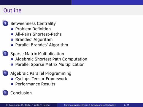
Outline

1 Betweenness CentralityProblem DefinitionAll-Pairs Shortest-PathsBrandes’ AlgorithmParallel Brandes’ Algorithm

2 Sparse Matrix MultiplicationAlgebraic Shortest Path ComputationParallel Sparse Matrix Multiplication

3 Algebraic Parallel ProgrammingCyclops Tensor FrameworkPerformance Results

4 Conclusion

E. Solomonik, M. Besta, F. Vella, T. Hoefler Communication-Ecient Betweenness Centrality 2/21

Betweenness Centrality Problem Definition

Centrality in Graphs

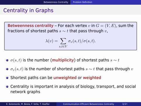
Betweenness centrality – For each vertex v in G = (V,E), sum thefractions of shortest paths s ∼ t that pass through v,

λ(v) =∑s,t∈V

σv(s, t)/σ(s, t).

σ(s, t) is the number (multiplicity) of shortest paths s ∼ t

σv(s, t) is the number of shortest paths s ∼ t that pass through v

Shortest paths can be unweighted or weighted

Centrality is important in analysis of biology, transport, and socialnetwork graphs


Betweenness Centrality Problem Definition

Path Multiplicities

Let d(s, t) be the shortest distance between vertex s and vertex t

The multiplicity of shortest paths σ(s, t) is the number of distinctpaths s ∼ t with distance d(s, t)

If v is in some shortest path s ∼ t, then

d(s, t) = d(s, v) + d(v, t)

Consequently, can compute all σv(s, t) and λ(v) given all distances

σv(s, t) =

σ(s, v)σ(v, t) : d(s, t) = d(s, v) + d(v, t)

0 : otherwise


Betweenness Centrality All-Pairs Shortest-Paths

Betweenness Centrality by All-Pairs Shortest-Paths

We can obtain d(s, t) for all s, t by all-pairs shortest-paths (APSP)

Multiplicities (σ and σv for each v) are easy to get given distances

However, the cost of APSP is prohibitive, for n-node graphs:

Q = Θ(n3) work with typical algorithms (e.g. Floyd-Warshall)

D = Θ(log(n)) depth1

M = Θ(n2/p) memory footprint per processor

APSP does not eectively exploit graph sparsity

1Tiskin, Alexander. "All-pairs shortest paths computation in the BSP model."Automata, Languages and Programming (2001): 178-189.E. Solomonik, M. Besta, F. Vella, T. Hoefler Communication-Ecient Betweenness Centrality 5/21

Betweenness Centrality Brandes’ Algorithm

Brandes’ Algorithm for Betweenness Centrality

Ulrik Brandes proposed a memory-ecient method1

Compute d(s, ?) and σ(s, ?) for a given source vertex s

Using these calculate partial centrality factors ζ(s, v) so

ζ(s, v) =∑

t∈V, d(s,v)+d(v,t)=d(s,t)

σ(v, t)/σ(s, t)

Construct the centrality scores from partial centrality factors

λ(v) =∑s

σ(s, v)ζ(s, v)

1Brandes, Ulrik. "A faster algorithm for betweenness centrality." Journal ofmathematical sociology 25.2 (2001): 163-177.E. Solomonik, M. Besta, F. Vella, T. Hoefler Communication-Ecient Betweenness Centrality 6/21


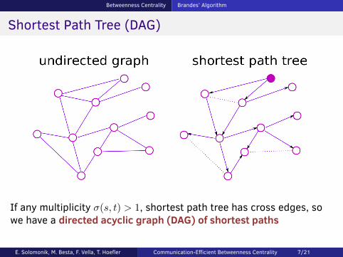
Shortest Path Tree (DAG)

If any multiplicity σ(s, t) > 1, shortest path tree has cross edges, sowe have a directed acyclic graph (DAG) of shortest paths



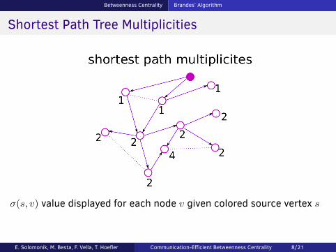
Shortest Path Tree Multiplicities

σ(s, v) value displayed for each node v given colored source vertex s



Partial Centrality Factors in Shortest Path Tree

If π(s, v) are the children of v in shortest path tree from s

ζ(s, v) =∑

c∈π(s,v)

(1

σ(s, c)+ ζ(s, c)

)



Brandes’ Algorithm Overview

For each source vertex s ∈ V (or a batch of source vertices)

Compute single-source shortest-paths (SSSP) from s

For unweighted graphs, use breadth first search (BFS)

More viable choices for weighted graphs: Dijkstra, Bellman-Ford,∆-stepping, ...

Perform back-propagation of centrality scores on shortest pathtree from s

Roughly as hard as BFS regardless of whether G is weighted


Betweenness Centrality Parallel Brandes’ Algorithm

Parallelism in Brandes’ Algorithm

Sources of parallelism in Brandes’ algorithm:

Computation of SSSP and back-propagation

Concurrency and eciency like BFS on graphs

Bellman-Ford provides maximal concurrency for weighted graphs atcost of extra work

Dierent source vertices can be processed in parallel as a batch

Key additional source of concurrency

Maintaining more distances requires greater memory footprint,M = Ω(bn/p) for batch size b


Sparse Matrix Multiplication Algebraic Shortest Path Computation

Algebraic shortest path computations

Tropical (geodetic) semiring

additive operator: a⊕ b = min(a, b), identity: ∞

multiplicative operator: a⊗ b = a+ b, identity: 0

semiring matrix multiplication:

C = A⊗B ⇒ cij = mink

(aik + bkj)

Bellman-Ford algorithm (SSSP) for n× n adjacency matrix A:

1 initialize v(1) = (0,∞,∞, . . .)

2 compute v(n) via recurrence

v(i+1) = v(i) ⊕ (A⊗ v(i))


Sparse Matrix Multiplication Algebraic Shortest Path Computation

Algebraic View of Brandes’ Algorithm

Given frontier vector x(i) and tentative distances w(i)

y(i) = A⊗ x(i) and w(i+1) = w(i) ⊕ y(i)

x(i+1) given by entries if w(i+1) that dier from w(i)

For BFS, tentative distances change only once

For Bellman-Ford, tentative distances can change multiple times

At maximum as many times as the depth of the shortest path DAG

Thus both algorithms require iterative SpMSpV

Having a batch size b > 1 transforms the problem to sparse matrixmultiplication (SpGEMM or SpMSpM)


Sparse Matrix Multiplication Parallel Sparse Matrix Multiplication

Communication Avoiding Sparse Matrix Multiplication

Let the bandwidth costW be the maximum amount of datacommunicated by any processor

We use analogue of 1D/2D/3D rectangular matrix multiplication

The bandwidth cost of matrix multiplication Y = AX is then

W = minp1p2p3=p

[nnz(A)

p1p2+

nnz(X)

p2p3+

nnz(Y )

p1p3

])In our context, nnz(A) = |E| = m, while X holds current frontiersfor b starting vertices, so nnz(X) ≤ nb


Sparse Matrix Multiplication Parallel Sparse Matrix Multiplication

Communication Avoiding Betweenness Centrality

Latency cost is proportional to number of SpMSpM calls

Replication of A for SpMSpMs minimizes bandwidth costW

It then suces to communicate frontiers X and reduce results Y

For undirected graphs, for b starting vertices, total nonzeros in Xover all iterations is nb and for Y is O(nb)

Best choice of b with sucient memory gives

W = O(n√m/p2/3)

Memory-constrained communication cost bound given in paper

Perfect theoretical strong scaling in communication cost

from p0 to Θ(p3/20 n2/m) processors


Algebraic Parallel Programming Cyclops Tensor Framework

Cyclops Tensor Framework (CTF) 1

Distributed-memory symmetric/sparse tensors in C++ or Python

For betweenness centrality, we only use CTF matricesMatrix <int > A(n, n, AS|SP, World(MPI_COMM_WORLD ));A.read(...); A.write(...); A.slice(...); A.permute(...);

Matrix summation in CTF notation isB["ij"] += A["ij"];

Matrix multiplication in CTF notation isY["ij"] += T["ik"]*X["kj"];

Used-defined elementwise functions can be used with eitherY["ij"] += Function <>([]( double x) return 1/x; )(X["ij"]);Y["ij"] += Function <int ,double ,double >(...)(A["ik"],X["kj"]);

1E. Solomonik, D. Matthews, J. Hammond, J. Demmel, JPDC 2014E. Solomonik, M. Besta, F. Vella, T. Hoefler Communication-Ecient Betweenness Centrality 16/21


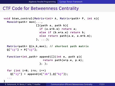
CTF Code for Betweenness Centrality

void btwn_central(Matrix <int > A, Matrix <path > P, int n)Monoid <path > mon(...,

[]( path a, path b)if (a.w<b.w) return a;else if (b.w<a.w) return b;else return path(a.w, a.m+b.m);

, ...);

Matrix <path > Q(n,k,mon); // shortest path matrixQ["ij"] = P["ij"];

Function <int ,path > append ([]( int w, path p)return path(w+p.w, p.m);

; );

for (int i=0; i<n; i++)Q["ij"] = append(A["ik"],Q["kj"]);

...E. Solomonik, M. Besta, F. Vella, T. Hoefler Communication-Ecient Betweenness Centrality 17/21


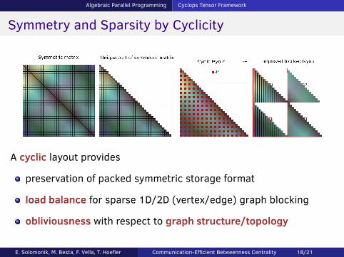
Symmetry and Sparsity by Cyclicity

A cyclic layout provides

preservation of packed symmetric storage format

load balance for sparse 1D/2D (vertex/edge) graph blocking

obliviousness with respect to graph structure/topology



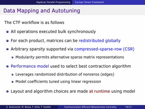
Data Mapping and Autotuning

The CTF workflow is as follows

All operations executed bulk synchronously

For each product, matrices can be redistributed globally

Arbitrary sparsity supported via compressed-sparse-row (CSR)

Modularity permits alternative sparse matrix representations

Performance model used to select best contraction algorithm

Leverages randomized distribution of nonzeros (edges)

Model coecients tuned using linear regression

Layout and algorithm choices are made at runtime using model


Algebraic Parallel Programming Performance Results

CTF Performance for Betweenness Centrality

Implementation uses CTF SpGEMM adaptively with sparse ordense output (push or pull)We compare with CombBLAS, which uses semirings and BFS(unweighted only)

1

4

16

64

256

2 8 32 128

MTE

PS

/nod

e

#nodes

Strong scaling of MFBC for real graphs

Friendster CTF-MFBCOrkut CTF-MFBC

LiveJournal CTF-MFBCPatents CTF-MFBC

4

16

64

256

1024

4096

2 8 32 128

MTE

PS

/nod

e

#nodes

Strong scaling for R-MAT S=22 graph

E=128 CTF-MFBC unweightedE=128 CombBLAS unweighted

E=128 CTF-MFBC weightedE=8 CTF-MFBC unweightedE=8 CombBLAS unweighted

E=8 CTF-MFBC weighted

Friendster has 66 million vertices and 1.8 billion edges (results onBlue Waters, Cray XE6)


Conclusion

Conclusions and Future Work

Summary of algorithmic contributionsParallel communication-avoiding betweenness centrality algorithmBetter sparse matrix multiplication for unbalanced nonzero countsAlgorithms and implementation general to weighted graphs

Future workUse of ∆-stepping or other more work-ecient SSSP algorithmsOptimizations in conjunction with approximation algorithms

Cyclops Tensor FrameworkGraphs are one of many applications, other highlights include

Petascale high-accuracy quantum chemistry56-qubit (largest ever) quantum computing simulation

Already provides most functionality proposed in GraphBLAS 1,plus all of that for tensors (hypergraphs with uniform size nets)


Scaling Betweenness Centrality using Communication ...

Documents

Transcript of Scaling Betweenness Centrality using Communication ...