• Scale physical model

• Mathematical model

• Numerical model

How to Model Physical Systems

www.autospeed.com

• Develop mathematical models, i.e. ordinary differential equations that describe the relationship between input and output characteristics of a system.

• These equations can then be used to forecast the behaviour of the system under specific conditions.

• All systems can normally be approximated and modelled by one of several models, e.g. mechanical, electrical, thermal or fluid. We also find that we can translate a system from one model to another to facilitate the modelling.

Modelling of Physical Systems

Lumped Parameter Models

• Use standard laws of physics and break a system down into a number of building blocks.

• Each of the parameters (property or function) is considered independently.

www.brains-minds-media.org

http://www.3me.tudelft.nl/en/about-the-faculty/departments/biomechanical-engineering/research/dbl-delft-biorobotics-lab/bipedal-robots/

Lumped Parameter Models

www.sozogaku.com/fkd/en/mfen

Millennium wobbly bridgehttp://www.youtube.com/watch?v=eAXVa__XWZ8

Linear Time Invariant Models

• Assume the property of linearity for these models.

• A linear system will posses two properties;

1. Superposition

2. Homogeneity.

Allows us to use standard mathematical operations to simplify our models

http://www.cyberphysics.co.uk/

www.redlinemotive.com

Linear Time Invariant Models

• Assume system is time-invariant

• Constants stay constant in the time-scales of our model

• Proportionality between variables does not change.

Our shock absorbers do not wear in our car suspension model!

Competition tyres

Elements of Systems are Ideal • Each element completely describes a property

• Elements are:

• Ideal

• Linear

• Represent only one property

The Spring ElementRepresents the elastic properties (energy storage) in a system.

Assume:

• No mass

• No Fraction

• Linear

Hooke’s Law: f(t) = K(x1 – x2) = Kx(t)

f(t) = force applied to the ends of the spring, K = spring constant (N.m) or C = 1/K is the spring compliance,x1 = Displacement of the one end, x2 = Displacement of the other end,

x = x1 – x2 = relative displacement of the two ends. Rotational spring element torque T(t) in terms of the angular displacement :

  T(t) = K(1 - 2) = K(t) T(t) = Torque(t) = angular displacement

The Spring Element

Real springs show deviation from ideal:

• Real springs would have an associated mass, leading to the deviations in the step and sinusoidal response as described before.

• Real springs will always contain some friction (energy dissipation) which is exhibited in the non-coincidence of the loading – unloading curves.

• Real springs will always exhibit a degree of non-linearity (deviation from f = Kx). See section on linearisation.

The Spring Element

Energy losses in real springs

Several types of practical springs

marccardaronella.com

Linearisation Many elements show non-linear behaviour.

To use in our relatively simple models, we must first linearise this element around an operating point.

Get a linear model that should be valid for small excursions from this operating point.

Consider a non-linear coil spring that forms part of the suspension system of an automobile.

Operating point = Equilibrium position under load

Example: Consider f(x) = 2x + 5x3

f(x) = f(2 (xo)+5(xo)3) + f’(2 +3.5 xo 2).(x-1)

f(x) = f(2 (1)+5(1)3) + (2 +3.5.12)(x-1)

Linearise: Intuitively with tangent

Or Taylor series:

A finite number of terms will give an approximation of the function – the first two terms will give a linear approximation

Example: Consider f(x) = 2x + 5x3

Operating point x = 1: f(x) ~ -10 + 17x

Model the spring force as f(x) = -10 + 17x around the point x = 1.0 and

the linearised spring forced constant would be given by df/dx = 17 N/m.

Linearisation

...

!20

2

2

00

00

xx

dx

ydxx

dx

dyxfy

xx

The Damper ElementDamper element (dashpot) represents the forces opposing motion, i.e. the friction or damping effects.

Damping force is proportional to the velocity of the piston.

where f = force applied to the ends of the damper,

dx/dt = v = relative velocity of the plunger

fv = coefficient of viscous friction or simply called the damping coefficient

vfdt

dxf

dt

dx

dt

dxff vvv

21

The Damper Element

http://www.flotronicpumps.co.uk/

www.modified.com

The Mass (inertia) ElementAll real elements will have some mass, so that the mass element in the model will thus represent the physical mass of the system.

This element represents the inertia or resistance to acceleration of the system.

The mass element will be modelled as concentrated at a point.

The three solutions • stiffening the structure, • dampening structural vibration, • limiting/modifying bridge traffic Estimates place the cost of the stabilization work in the neighborhood of £5 million.(Source: http://pub20.ezboard.com/fglobalarchitectureforumsother.showMessage?topicID=145.topic)

Millennium Bridge London

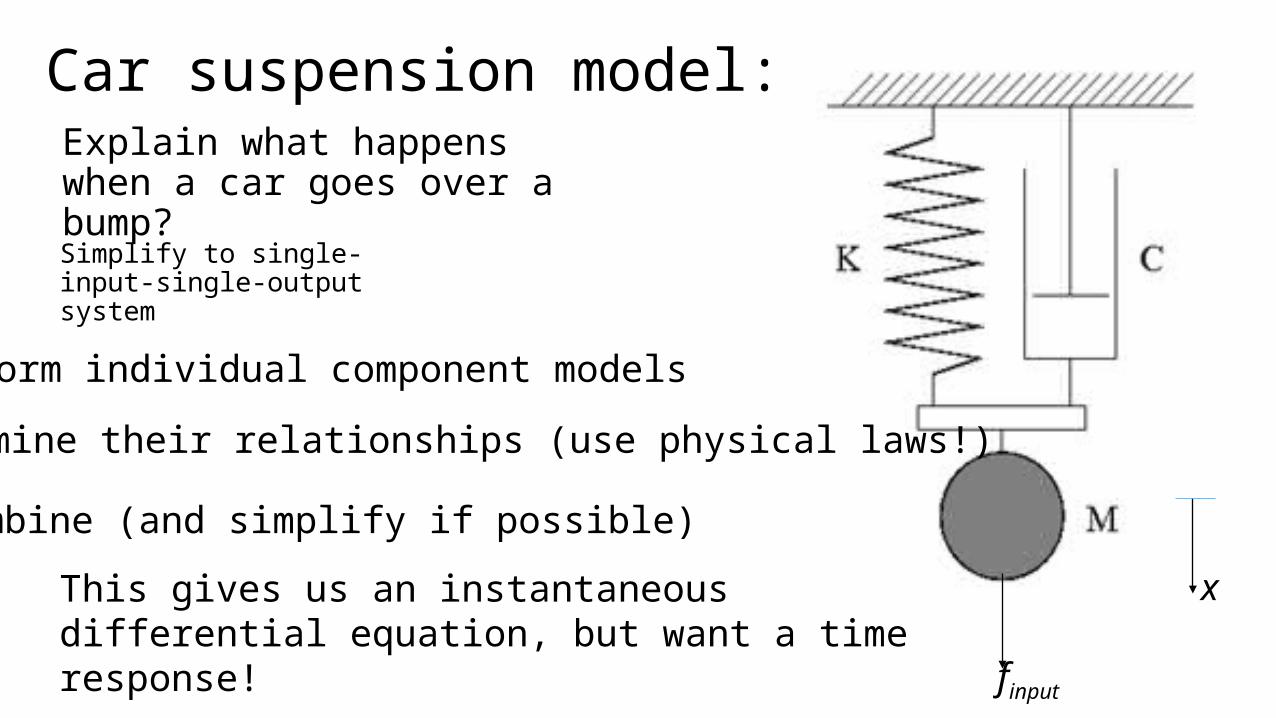
Car suspension model:

• Mechanical system

Explain what happens when a car goes over a bump?

www.superbike-coach.com

Car suspension model:Explain what happens when a car goes over a bump?

x

finput

Simplify to single-input-single-output system

Form individual component models

Determine their relationships (use physical laws!)

Combine (and simplify if possible)

This gives us an instantaneous differential equation, but want a time response!

Spring

Damper

Mass

Source Nise 2004

Force - Distance

tKxtf s

dt

tdxCtfc

2

2

dt

txdMtfm

tf

tx

tf

tx

tf

tx

tftftftf mdsinput

Car suspension model:

2

2

dt

txdm

dt

tdxCtKxtfinput

This gives us an instantaneous differential equation, but want a time response!

Integrate:• numerically• theoretically• using tables

clf; %clear all graphs K = 10 %Spring constantC = 3 %Damping constantm = 1 %mass (constant)

t = [0: 0.01: 20];%set up the time incrementsstept = 1 + 0*t; %graph to show step responseplot(t,stept,'m');xlabel('Time t (s)')ylabel('Distance x (m)')

hold on % put each graph on top of each other

for C = 1.0: 1: 10.0d = tf(9,[m C K]) [y,t]=step(d,T);%step response over one secondplot(t,y,'k');pause(2)

end

0 2 4 6 8 10 12 14 16 18 200

1

2

3

4

5

6

7

8

9

Time t (s)

Dis

tanc

e x

(m)

0 2 4 6 8 10 12 14 16 18 200

0.5

1

1.5

Time t (s)

Dis

tanc

e x

(m)

0 2 4 6 8 10 12 14 16 18 200

0.5

1

1.5

Time t (s)

Dis

tanc

e x

(m)