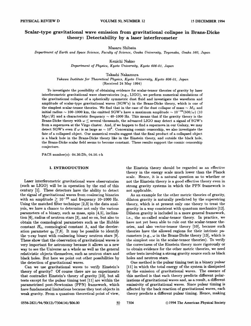
PHYSICAL REVIEW D VOLUME 50, NUMBER 12 15 DECEMBER 1994

Scalar-type gravitational +rave emission from gravitational collapse in Brans-Dicketheory: Detectability by a laser interferometer

Masaru ShibataDepartment of Earth and Space Science, Eaculty of Science, Osaka Unioersity, Toyonaka, Osaka 560, Japan

Kenichi NakaoDepartment of Physics, Kyoto University, Kyoto 606 01, -Japan

Takashi NakamuraYukawa Institute for Theoretical Physics, Kyoto University, Kyoto 606 01, J-apan

(Received 24 May 1994)

To investigate the possibility of obtaining evidence for scalar-tensor theories of gravity by laserinterferometric gravitational wave observatories (e.g. , LIGO), we perform numerical simulations ofthe gravitational coQapse of a spherically symmetric dust auid and investigate the waveform andamplitude of scalar-type gravitational waves (SGW s) in the Brans-Dicke theory, which is one ofthe simplest scalar-tensor theories. We find that in the case of the dust collapse of mass Mo andinitial radius 100—1000 km, the emitted SGW's have a maximum amplitude 10 (500/u) (10Mpc/A) and a characteristic frequency 40—1000 Hz. This means that if the gravity theory is theBrans-Dicke theory with ~ & several thousands, the advanced LIGO may detect a signal of SGW'sfrom a supernova at the Virgo cluster. And, if we happen to find a supernova in our Galaxy, we maydetect SGW's even if u is as large as 10 . Concerning cosmic censorship, we also investigate thefate of a collapsed object. Our numerical results suggest that the final product of a collapsed objectis a black hole in the Brans-Dicke theory like in the Einstein theory, and outside the black hole,the Brans-Dicke scalar field seems to become constant. These results support the cosmic censorshipconjecture.

PACS number(s): 04.30.Db, 04.50.+h

I. INTRODUCTION

Laser interferometric gravitational wave observatories(such as LIGO) will be in operation by the end of thiscentury [1]. These detectors have the ability to detectthe signal of gravitational waves from coalescing binarieswith an amplitude & 10 and &equency 10—1000 Hz.Using the matched filter technique [2,3] in the data anal-ysis, we have a chance to determine not only the variousparameters of a binary, such as mass, spin [4,5], inclina-tion [6], radius of neutron stars [3], and so on, but also toobtain the cosmological parameters such as the Hubbleconstant Ho, cosmological constant A, and the deceler-ation parameter qo [7,8]. It may be possible to identifythe p-ray burst with coalescing binary neutron stars [9].These show that the observation of gravitational waves isvery important for astronomy because it allows us a new

way to see the Universe as a whole as well as the generalrelativistic objects themselves, such as neutron stars andblack holes. But here we point out other possibilities bythe detection of gravitational waves.

Can we use gravitational waves to verify Einstein'stheory of gravity'? Of course there are no experimentsthat contradict Einstein's theory of gravity [10], but alltests except for the pulsar timing test [11]are within theparametrized post-Newtonian (PPN) framework, whichhave fundamental limitations because they test objects inweak gravity. From a quantum theoretical point of view,

the Einstein theory should be regarded as an effectivetheory in the energy scale much lower than the Planckscale. Hence, it is a natural question as to whether ornot the Einstein theory is a good effective theory even instrong gravity systems in which the PPN framework isnot applicable.

As an example for the other metric theories of gravity,dilaton gravity is naturally predicted by the superstringtheory, which is at present only one theory to treat thegravity in a way consistent with quantum mechanics [12].Dilaton gravity is included in a more general &amework,i.e., the so-called scalar-tensor theory. In practice, we

have not yet been able to rule out the scalar-tensor the-ories, and also vector-tensor theory [10], because suchtheories have the allowed regions for their intrinsic pa-rameters (e.g. , u in the Brans-Dicke theory [13],which isthe simplest one in the scalar-tensor theories). To verifythe correctness of the Einstein theory more rigorously orto obtain evidence for the other metric theories, we needother tests involving a strong gravity source such as blackholes and neutron stars.

One method is the pulsar timing test in a binary pulsar[ll] in which the total energy of the system is dissipatedby the emission of gravitational waves. The essence ofthis method is that each theory predicts different polar-izations of gravitational waves and, as a result, a diferentemissivity of gravitational waves. Since pulsar timing isaffected by the back reaction of gravitational waves, eachtheory predicts a djtfferent pulsar timing. Hence, making

0556-2821/94/50(12)/7304(14)/$06. 00 50 7304 Qc 1994 The American Physical Society

50 SCALAR-TYPE GRAVITATIONAL VfAVE EMISSION PROM. . . 7305

use of the binary pulsar, especially using a black-hole—neutron-star binary pulsar, we can test the metric theorymore rigorously [10,14]. However, for a rigorous test, weneed black-hole —neutron-star binaries or binary neutronstars of a large mass ratio in our Galaxy [14],which havenot been found yet.

The second possibility to investigate the metric the-ory is the direct detection of gravitational waves, whichmay include various types of polarization [15,16]. For ex-ample, let us consider the Brans-Dicke theory (or scalar-tensor theory), which is our subject in this paper. In thiscase, there are three polarization modes: Two of themare the same as those in the Einstein theory, that is, theso-called + and x modes, but there exists one additionalmode, the scalar (spin-zero) mode, which is emitted evenin the spherically symmetric space-time. Thus, theoret-ically, if we can detect scalar-type gravitational waves(SGW's) with a laser interferometric detector, we maysay that the scalar-tensor theory is correct. Also, if wedo not detect the scalar mode but do detect only + andx modes, it has an important meaning because we canexclude the scalar-tensor theory within the sensitivity ofthe detector.

In practice, there may be maximally six polarizationmodes in gravitational waves if we take into account thevarious theories [15,10]. In this case we need at leastsix detectors operating at the same time and at ddfer-ent places to distinguish every mode. Hence, it seemsimpossible to distinguish the scalar mode kom the vari-ous other modes unless we Snd a strong periodic sourceof gravitational waves [10]. However, as shown in thispaper, the characteristic amplitude and frequency of thescalar mode may be difFerent &om those of the othermodes in some sources of gravitational waves. Thismeans that several characteristic peaks may appear inthe spectr»m of gravitational waves. Since the interfero-metric gravitational wave detector has a wide &equencyband, it has the ability to detect the various types ofwaves of diferent characteristic &equencies and wave-forms. Hence, we may be able to distinguish the scalarmode &om the other modes completely by making use ofthe features of these modes.

From the above point of view, a supernova (SN), whichis considered a weak emitter of gravitational waves in thecase of the Einstein theory [17], becomes an importantsource of SGW's because the scalar mode is emitted even&om spherically symmetric collapse. We can think asfollows: If signals of SGW's &om a SN are detected, wecan verify the scalar-tensor theory, and, even if no signalsof SGW's are detected &om the SN, which is seen byelectromagnetical observations, we may give the upperlimit of the intrinsic parameter of the theory, e.g. , ~ inBrans-Dicke theory. Thus, the absence of a signal maylead to the restriction of the theory.

This is the reason we perform the n»merical simula-tion of the gravitational collapse and investigate the am-plitude and the kequency of SGW's in the Brans-Dicketheory to see the possibility in detecting gravitationalwaves other than the + and x modes. Although thereare many alternative scalar-tensor theories in addition tothe Brans-Dicke theory, which is consistent with the PPN

II. BASIC EQUATIONS AND NUMERICALMETHOD

A. Basic equations

The basic equations of the Brans-Dicke theory [13] areoriginally expressed in the Brans-Dicke &arne, and theyhave the form

R s —2g sR=Sng Ts+~4 '(Vo4Vs4 zgosg"V. 4—V~—4)+y '(V.Vsy —g.sV.V'4), (2.1)

V V Q = Sz (2u) + 3) T (2.2)

and

V T~ ——0, (2.3)

where g g is the metric in the Brans-Dicke kame, andB g, B, and V are the Ricci tensor, Ricci scalar, andcovariant derivative with respect to g ~, respectively. T pis the energy-momentnm tensor, and P is the Brans-Dickefield by which the locally measured gravitational constantcan be written as

g24p+ 4

2'+ 3 (2.4)

Dicke has pointed out [20] that the theory can also beexpressed in another kame, the so-called Einstein kame,and in this kame, the equations become

experiment [10,18], we only pay attention to the Bra~~-Dicke theory because our intent here is to show that it ispossible to detect SGW's &om the SN source. Hence, wealso do not intend to calculate the detailed dynamics ofthe gravitational collapse and waveforms of SGW's. Thedetailed calculations will be future problems.

The remainder of this paper is devoted to the detailsunderlying the above discussion. In Sec. II, we derivethe equations for the spherical symmetric gravitationalcollapse in the Brans-Dicke theory, and the numericalmethods are also shown. In Sec. III we first show thenumerical results, in particular, the waveforms and theFourier spectra of SGW's for various models. Even if theSGW has a high enough amplitude to be detected by theinterferometric detector, it is nontrivial whether or notthe detector has the ability to detect SGW's. Thus, in thelatter half of Sec. III, we show that it is possible to detectSGW's with a laser interferometric detector. To makesure of the cosmic censorship hypothesis [19],in Sec. IV,we brie8y show that the Bnal fate of the collapsing objectsis a black hole by means of the apparent horizon search.Section V is devoted to the snmmary. Throughout thispaper, we take the units of c = G = 1 and Mo denotesthe solar mass.

7306 MASARU SHIBATA, KENICHI NAKAO, AND TAKASHI NAKAMURA 50

R g—2g gR=87lC Tg

= ~'(Vo@Vs4 ——,'g sg'"V, @VLCC ), (2.5)

Then the equations of the dust become

Bt,D+ (—r DVi) „=0 (2.14)

and

(2.6)1

OqSi + —s(r SiVi) „= —2S aa „e

V Ts = 2(V O)TP —2i(Vs@)T (2 7)

where u' = ~ + 2, 4 = ln(P), and g s = Pg s. R q, R,and V are the Ricci tensor, Ricci scalar, and covariantderivative with respect to g s, respectively.

Here, in the Einstein kame, the equations are essen-tially the same as the Einstein equation with a scalarfield 4', while the equations in the Brans-Dicke frameare somewhat complicated because they include the sec-ond derivatives of P in the right-hand side (RHS) of Eq.(2.1). Hence for convenience of numerical computation,we solve the equations in the Einstein frame.

We numerically treat the spherically symmetric dustcollapse in the Brans-Dicke theory. In numerical calcu-lation, we use the 3+1 formalism and choose the lineelement (i.e., the gauge condition) as

where y = r . S becomes

S = — e~D2 + e2~A —2yS20 1

t9g4—

o.B2O,g = 4y@yy+ 6@y

fa„B„+4y@y '" + 2

Av~ 4n D2+-A )

~' So

The equation of the scalar field becomes

(2.16)

(2.17)

ds = adt —+A dr +B r (d8 +sin ed' ) . (2.8)

PaA A A

Tab = ~au& ) (2.9)

As for the time coordinate, we adopt the maximal slic-ing condition, K = 0. Then, in the above gauge,K = Bg(AB )/A—B, so that AB is constant with re-spect to the time t and depends only on the radial coor-dinate r

The energy-momentum tensor of the dust fiuid is writ-ten as

To solve the metric and extrinsic curvature, we haveseveral choices to treat the equations in the Brans-Dicketheory because they also have the constraint equationsas well as the evolution equations. Here we adopt thefollowing method: (1) As for the three-metric, we solvethe evolution equation of A, so that B is obtained &omAB = vPs(r) = const, where Q is fixed at the stage of theinitial value equations (see below); (2) as for the extrinsiccurvature K„"(=Ki), we solve the momentum constraintequation; (3) the Hamiltonian constraint is used to checkthe accuracy.

Then the basic equations become

V (pu ) = 2(V 4)pu (2.10)

Thus, we define p = pe 2 . In this case the equationbecomes the conservative form

where p and u are the baryon mass density and thefour-velocity in the Brans-Dicke frame. This means that—u u does not become unity but P in the Einsteinkame. Furthermore, the equation for p does not becomea fiux conservative equation. Instead, it becomes

0~A = —o.K~A,

( B„A,„~4/el yy + 6' y + 4go.' y 2

A

(2.18)

(2.19)

V (pu)=0. (2.11) = 4' O! + + —&Kg A + 4) 0,'/Apse ~ ASViy) 3 . . . g'

Taking into account these facts, we define the Huid vari-ables as

pp, = pAB (au ), S„=aAB pu u„,(2.12)

Si ——S„/r, Vi ——V"/r . (2.13)

D=aAB pu, S =Du, V"= „"u A

We also define the following quantities to guarantee theregularity at r = 0:

(2.20)

Ki ——r B dr r A B[8vrSi —2~'g4, &] . (2.21)0

The first equation is the evolution equation of A. Thesecond and third equations are obtained &om the max-imal slicing condition K = 0. The fourth equation isobtained &om the momentum constraint.

50 SCALAR-TYPE GRAVITATIONAL WAVE EMISSION FROM. . . 7307

To obtain the initial condition, we must solve theHamiltonian constraint. By virtue of the spherical sym-metry, we can consider, without loss of generality, theconformally flat initial condition A = B = $2. Then, inthis case, the Ham~&tonian constraint becomes

4yvj „„+6@„=—2z ——Q K~phe

I

[—~'—@ '+4(@, )'yW]. (2.22)

Before proceeding further, we brieQy review the be-havior of the metric in the wave zone [16]. Since met-ric quantities, a, A, and B, do not contain the wavelikecomponent in the wave zone, in the Brans-Dicke frame(denoted by Ch), the line element in this zone becomes

p:(p) I I I I I I

-.5

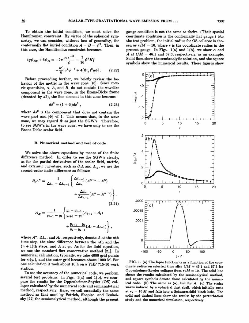
gauge condition is not the same as theirs. (Their spatialcoordinate condition is the conformally fiat gauge. ) Forthe test problem, the initial radius for OS collapse is cho-sen as r/M = 10, where r is the coordinate radius in thepresent gauge. In Figs. 1(a) and 1(b), we show a andA at t/M = 46.1 and 57.3, respectively, as an example.Solid lines show the semianalytic solution, and the squaresymbols show the numerical results. These figures show

ds = (1+4)ds (2.23) -1.5where ds2 is the component that does not contain thewave part and ~4~ (( 1. This means that, in the wavezone, we may regard 4 as just the SGW's. Therefore,to see SGW's in the wave zone, we have only to see theBrans-Dicke scalar field.

-2

.6

I I I I I I I I I I

5 10 15 20

B. Numerical method and test of code

We solve the above equations by means of the finitedifference method. In order to see the SGW's clearly,as for the partial derivatives of the scalar field, metric,and extrinsic curvature, such as 8&A and A,„,we use thesecond-order finite difFerence as follows:

An I ~—& (Ara+1 Are)6t„+Et„,~

Et„

.2

p I I I I I I I t I I t i i i T i i T T

0 5 10 15 20

(A" —A" z)Lt„

b,t„(2.24)

A„= t ' ' '(A,+, —A, )y'+i —y*' [ y~+i —y'

+ '+ '(A —A )I9' —9'—i

~ 0002 gl:(e)

.00015—

.0001

I I I I I I;i., I I I I I I I I I

where A", 6 t„, and A;, respectively, denote A at the nthtime step, the time cMerence between the nth and the(n+ 1)th steps, and A at y;. As for the fiuid equation,we use the standard flux conservative method [21]. Innumerical calculation, typically, we take 4000 grid pointsfor r;(y;), and the outer grid becomes about 1000 M. Forone calculation it took about 10 h on a YHP 715-50 workstation.

To see the accuracy of the numerical code, we performseveral test problems. In Figs. 1(a) and 1(b), we com-pare the results for the Oppenheimer-Snyder (OS) col-lapse calculated by the m~~erical code and semianalyticalmethod, respectively. Here, we call essentially the s~memethod as that used by Petrich, Shapiro, and Teukol-sky [22] the semianalytical method, although the present

-100 -5Q Q 50 100t- r*

FIG. 1. (a) The lapse function a ss a function of the coor-dinate radius on selected time slice t/M = 46.1 and 57.3 forOppenheimer-Snyder collapse &om r/M = 10. The solid lineshows the results calculated by the semiaualytical method,and square symbols denote those calculated by the n~~mer-ical code. (b) The same as (a), but for A. (c) The sca&~rwaves induced by a spherical dust shell, which initially restsat r, = 10M and fe&&~ into a Schwarsschild black hole. Thesolid and dashed lines show the results by the perturbationstudy and the numerical simulation, respectively.

7308 MASARU SHIBATA, KENICHI NAKAO, AND TAKASHI NAKAMURA 50

that the present niimerical method works well.%e also perform the comparison of wave forms of scalar

waves calculated by the perturbation study around aSchwarzschild black hole and by numerical simulation.Here, the method of the perturbation study is essentiallythe same as the perturbation study of gravitational wavesaround a black hole. (See, for example, Ref. [26].) In Fig.1(c), we show the numerical results of 4r at r 100 Minduced by a spherical dust shell, which initially rests atrg ——10M, where r~ is the areal radius and falls into aSchwarzschiid black hole. In this calculation, the massof the dust shell is set as y, = M/10, so that two resultsshould agree within an accuracy of 10'%%uo. In numericalsimulation, the black hole is expressed by the compactdust clump whose radius B 0.3M initially. In the fig-ure, solid and dashed lines show the results by the pertur-bation study and the numerical simulation, respectively.It is found that both results agree very well. This alsoshows that the present numerical method works well.

equilibrium state will be mainly determined by neutrinopressure [24]. In this case, the equation of state will be-come p pe/3 and T becomes —p. To take into accountthis property, we calculate the initial condition of 4 fromthe following equation, which is obtained from Eq. (2.17)inserting Bt,ri = rl = 0:

( cr„B„A„t4y@ yy + 64 y + 4y@ y

'" + 2

4~2(3 2)

Note that if we solve this equation, the asymptotic valueof 4 becomes M/rut'. In both cases, the momentumconstraint is satisfied automatically (Ki ——0) and wehave only to solve the Hamiltonian constraint to obtainthe initial condition.

III. NUMERICAL RESULTS B. Numerical results

A. Initial conditions

As for the initial density configuration of the dust,p~i& 0, we adopt

pI = p [1+exp&(u —ui)/2@2)] (3 I)

where p„yi, and y2 are constant &ee parameters. Sincewe treat the dust, we can freely scale the unit of mass.For convenience, we determine p, to fix M = 1. Hence,the remaining free parameters are yi and y2. In thecase of yi )) y~, the distribution is almost homogeneous,while, in the case of yi (& y2, it becomes a Gaussian-type distribution. Here, we must be careful to give theseparameters because, if we choose an inappropriate set ofthe parameters, the naked singularity due to the shell fo-cusing [23] appears during numerical simulations and thesimulation must be stopped before the SGW's propagateto the wave zone. Experimentally, we found that such asingularity seems to appear in the case of yi ( y2, so we

adopt parameters satisfying yi & y2.Before we give the initial condition of C and g, we

should note the following: In the initial data, there isno information about the equation of state for baryonicmatters, although we treat p = 0 dust in the dynamicalevolution. This means that we may consider our simula-tions as follows: For t ( 0, the matter is almost underthe equilibrium state (so rI = 0), and, for t & 0, the pres-sure is reduced to zero and the collapse begins. Takinginto account the above, we consider two types of initialconditions. We call them cases (A) and (B). As for case

(A), we use the initial condition, 4 = rI = 0. We adoptcase (A) just for simplicity, but we can regard it as thehighly relativistic initial condition because it is consistentwith T = —p(1+ e) + 3P = 0, where e is the internalenergy per baryon mass. As for case (B), we adopt themore realistic initial condition. In realistic situations ofstellar cores before collapse, the equation of state in the

i t' M i /lOMpc)@~10(0.002) I 10Mo) ( R (3 3)

TABLE I. Initial conditions for models (Al) —(AS) and(B1)-(B4).

Model(A1)(A2)(A3)(A4)(A5)(As)(A7)(As)(B1)(»)(B3)(B4)

500505

500500500500500500500500500

~yi15151515301010

301510

~@20.40.40.46

0.40.4

0.40.40.40.40.4

Pc7.4 x 107.4 x 1074x1064x109.0 x 102.6 x 102.2x10 '2.1 x 109.0 x 107.4 x 102.5 x 102.1 x 10

We have performed numerical computations for a va-riety of parametrs yi, y2, and ur' for both cases (A) and(B). We show the parameters as well as the density atthe center p for selected models in Table I. Since theunit of the density is 6.17 x 10 gcm (Mo/M), thecentral densities in the initial conditions are 1011 1014

gcm for M = 1Mo 10Mo.First, to see the effects of u' on the waveforms of

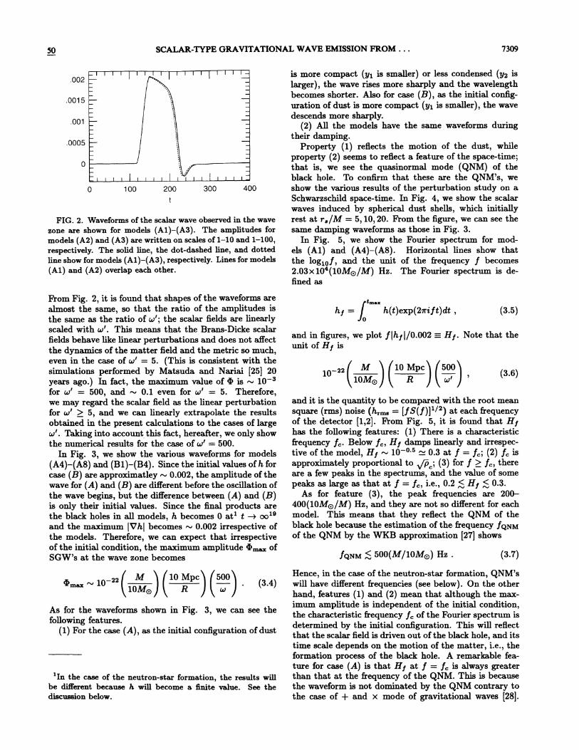
emitted SGW's, we compare the wave forms of models(Al) —(A3) in Fig. 2. The vertical axis corresponds to4(~'/500) at the numerical boundary. The solid line,dot-dashed line, and dashed line show the waveforms ofmodels (Al) —(A3). We note that the unit of the time tis 4.93x10 (M/10Mo) sec. Amplitudes of SGW's areshown in units of h = 4(R/M), where R is the arealradius &om the detector to the source. Hence, the am-plitude at the detector becomes

50 SCALAR-TYPE GRAUITATIONAL %'AVE EMISSION FROM. . . 7309

.002— I I I I I I I I I I

.0015—

.001

.0005—

I I I I I I I I I I

100 200

II & I I I

300 400

FIG. 2. Waveforms of the scalar wave observed in the wave

zone are shown for models (Al)—(A3). The amplitudes formodels (A2) and (A3) are written on scales of 1-10and 1—100,respectively. The solid line, the dot-dashed line, and dottedline show for models (Al) —(A3), respectively. Lines for models

(Al) and (A2) overlap each other.

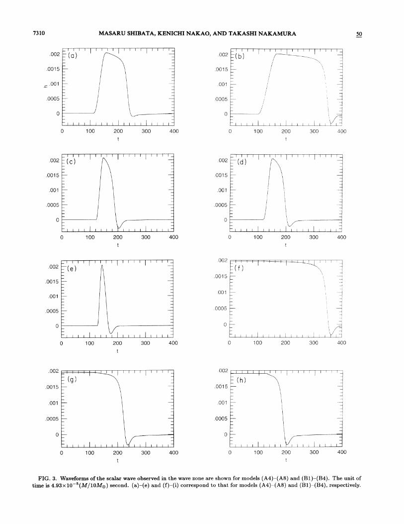
is more compact (yq is smaller) or less condensed (yz islarger), the wave rises more sharply and the wavelengthbecomes shorter. Also for case (B), as the initial config-uration of dust is more compact (yq is smaller), the wavedescends more sharply.

(2) All the models have the same waveforms duringtheir damping.

Property (1) refiects the motion of the dust, while

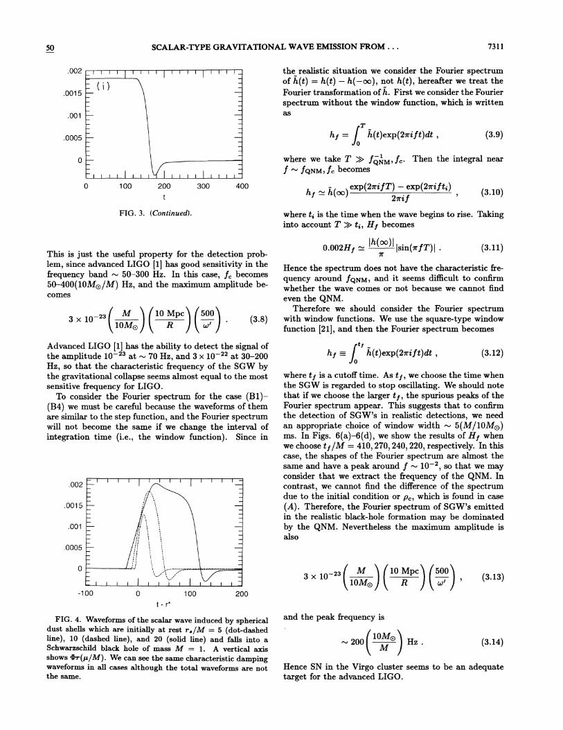
property (2) seems to refiect a feature of the space-time;that is, we see the quasinormal mode (QNM) of theblack hole. To co»&rm that these are the QNM's, we

show the various results of the perturbation study on aSchwarzschild space-time. In Fig. 4, we show the scalarwaves induced by spherical dust shells, which initiallyrest at r, /M = 5, 10, 20. From the figure, we can see thesame damping waveforms as those in Fig. 3.

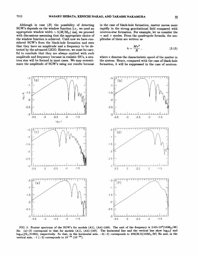
In Fig. 5, we show the Fourier spectrum for mod-els (Al) and (A4)—(AS). Horizontal lines show thatthe log&of, and the»»lt of the &equency f becomes2.03x104(10Mo/M) Hz. The Fourier spectr»m is de-fined as

From Fig. 2, it is found that shapes of the waveforms arealmost the same, so that the ratio of the amplitudes isthe same as the ratio of u'; the scalar fields are linearlyscaled with ~'. This means that the Brans-Dicke scalarfields behave like linear perturbations and does not afFectthe dynamics of the matter field and the metric so much,even in the case of u' = 5. (This is consistent with thesimulations performed by Matsuda and Nariai [25] 20years ago. ) In fact, the maxim»m value of O is ~ 10for u' = 500, and 0.1 even for a' = 5. Therefore,we may regard the scalar field as the linear perturbationfor u' & 5, and we can linearly extrapolate the resultsobtained in the present calculations to the cases of largew'. Taking into account this fact, hereafter, we only showthe n»merical results for the case of ur' = 500.

In Fig. 3, we show the various waveforms for models

(A4)—(A8) and (Bl)—(84). Since the initial values of h forcase (B) are approximatley ~ 0.002, the amplitude of thewave for (A) and (B) are di8'erent before the oscillation ofthe wave begins, but the &l&erence between (A) and (B)is only their initial values. Since the final products arethe black holes in all models, h becomes 0 at~ t + oops

and the maxim»m ~Vh~ becomes ~ 0.002 irrespective ofthe models. Therefore, we can expect that irrespectiveof the initial condition, the maxim»m amplitude @max ofSGW's at the wave zone becomes

&max

hy = h(t)exp(2z'i ft)dt,0

(3.5)

and in figures, we plot f[by[/0. 002 = Hy. Note that the»»t of Hy is

$0 22 M ~ (10 Mpc~ (500~

10Moj ( R ) (~') (3 6)

fclNM + 500(M/10Mo) Hz . (3 7)

and it is the quantity to be compared with the root meansquare (rms) noise (h, = [fS(f)]~~ ) at each &equencyof the detector [1,2]. From Fig. 5, it is found that Hyhas the following features: (1) There is a characteristicfrequency f, Below f„.Hy damps linearly and irrespec-tive of the model, Hy ~ 10 o s 0.3 at f = f, ; (2) f, isapproximately proportional to +p; (3) for f ) f„thereare a few peaks in the spectrums, and the value of somepeaks as large as that at f = f„i.e., 0.2 & Hy & 0.3.

As for feature (3), the peak &equencies are 200—400(10Mo/M) Hz, and they are not so difFerent for eachmodel. This means that they refiect the QNM of theblack hole because the estimation of the &equency fqNMof the QNM by the WKB approximation [27] shows

M ~ ~10 Mpc~ t 50014 10I10Mo) ( R ) ( ~ )

(3.4)

As for the waveforms shown in Fig. 3, we can see thefollowing features.

(1) For the case (A), as the initial configuration of dust

In the case of the neutron-star formation, the results willbe H&trent because h wi11 become a Snite value. See thediscussion below.

Hence, in the case of the neutron-star formation, QNM'swill have different &equencies (see below). On the otherhand, features (1) and (2) mean that although the max-im»m amplitude is independent of the initial condition,the characteristic &equency f, of the Fourier spectr»m isdetermined by the initial configuration. This will reBectthat the scalar field is driven out of the black hole, and itstime scale depends on the motion of the matter, i.e., theformation process of the black hole. A remarkable fea-ture for case (A) is that Hy at f = f is always greaterthan that at the &equency of the QNM. This is becausethe waveform is not doml»ated by the QNM contrary tothe case of + and x mode of gravitational waves [28].

731P MASARU SHIBATA , KENICHI NAKAO, AND TAKASHI NAKAMURA 5p

.002 —(0 )

.0015—

.001

.0005—

I I I I I I I I

.002 —(t )

.0015—

.001

.0005—

I I I I I

i

/

/

/

t

I

0

0 100I I I I I I I

200 300 400 0 100 200 300

.002 —(C)

.0015—

.001

.0005—

I I I I I I I I I I I I I

.002 —(d )

.0015—

.001

.0005—

0

0 100 200I I I I I I I

300 400 0 100 200 300 400

.002 —(e)

.0015—

.001

.0005—

I I I I I I I I

.001

.0005—

0

0I I I I I I I I

100 200I I I I I I I I

300 400 100 200 300 400

.002

.0015—

I I I I I

g)

.002 I I I I I I I I

—:(.0015—

.001 .001

.0005— .0005—

0 100 200 300 400 0 100 200I I

300 400

FIG. 3. Waveforms of the scalar wave observed in t e wave zone are shown for mode'(Mi oM ) ~ o d ( ) ( ) d(f) ()a e an —a correspond to that for models A4 —AS and (Bl)—(B4), respectively.

50 SCALAR-TYPE GRAVITATIONNAL WAVE EMISSION FROM. . . 7311

.002 I I

.0015—: (i

.001

I I I I I I I

)

I I I I I I I I the realistic situation we consider the Fof h(t) —h(t) h( —oo), not h(t), hereafter we trea

a iono . First we consnsider the Fourier

asi ou e window function hi h

'ou, w c is written

.0005—T

hy = h(t)exp(2wift)dh, (3.9)

where we take T » f . Th&NM, f, Th. en the integral nearecomes

I I I I I

100I I I I I I I I

200 300 400 exp(2n ifT) —exp(2s ift;)2+i f '7 (3.10)

FIG. 3. (Continued). where t is th e time when the wave be ins' t tT» t Hy becomes

This is just the usj he useful property for the detelem, since advanced LIGO [1] has

b d

comesz, and t e maximum amplitude be-

M ~ ~ 10 Mpcl (5O O

) &

(3.8)

.002— I I I I I I I I

.0015—

.001

.0005—

Advanced LIGO [1] has the abilit to g

H'' thtthe at~70Hz and

a e characteristic fre uench ' 1"0'' q y y

ona co apse seems almost e ualsensitive &equency for LIGO.

qu to the most

To consider t e ourier spectrump ~ ~ ( )-us e care because the w

are similar to th t fune waveforms of them

will not b ho e s ep function and t"the Fourier spectrum

gime i.e., the window function~ S'ince in

0.002' [sin(s T7r

(3.11)

Hence the spectrum does not have the cquency around

ve e characteristic fre-

qNM, and it seems difficult to nfirw et er the wave corn t beca

oco m

even the QNM.comes or not becat because we cannot Bnd

~ ~

erefore we should., h.;.dow f..„... ... hconsi er the F

en t e Fourier spectrum becomes

ty

hy = h(t)exp(2mi ft)dt, (3.12)

where tf is a cutofF time. As ty, we chooseegar e to stop oscillatin .

Fourier spectr»m a . hise e arger ty, the spurious peaks of the

th d t t'o of SGW' 'appear. his su e

o s in realistic detec'

h'

hoo t /M=41,0, 270, 240, 220 res

, th h fth Fsame and ha

s o e ourier s ecpectrum are almost the

(A). Th f th Fore, e ourier spectrum of Sth li t' bl k-h lac - o e formation

alsoevertheless the maximum amplitude is

0

I I I I

-100I I I I

100 200

M & )»Mp. &5001

10Mo) ( B )(3.13)

FIG. 4. ~. 4. Waveforms of the scalar vr

c are initially at rest rp enca

e orms xn all cases althou h thcteristxc damping

the same.es a ough the total waveforms are not

and the peak &equency is

10MO I

)Hz . (3.14)

Hence SN in thee Virgo cluster seems to betarget for the advanced LIGO

o e an adequate

7312 SIASARU SHIBATA, KBNICHI NAKAO, AND TAKASHI NAKASIURA 50

Although in case (B) the possibility of detectingSGW's depends on the window function [i.e., we need anappropriate window width 5(M/Mo) ms], we proceedwith discussions assuming that the appropriate choice ofthe window function is achieved. Until now we have con-sidered SGW's &om the black-hole formation and seenthat they have an amplitude and a frequency to be de-tected by the advanced LIGO. However, we must be care-ful to conclude that they are always emitted with suchamplitude and frequency becuase in reaIIstic SN's, a neu-tron star will be formed in most cases. We may overesti-mate the amplitude of SGW's using our results because

Mv2

R (3.15)

where v denotes the characteristic speed of the matter inthe system. Hence, compared with the case of black-holeformation, h will be suppressed in the case of neutron-

in the case of black-hole formation, matter moves morerapidly in the strong gravitational field compared withneutron-star formation For example let us consider the+ and x modes. From the quadrupole formula, the am-plitudes of them are written as

-5 I I I I I I I I I I I I I I I I I

C)

bQO -2

-15

-2.5—

-3.5 -3 -2.5 -2

logio f

I I I I I I

-1.5

-2.5

-3.5 -3 -2.5 -2 -1.5

-1.5

-2

-2.5—I

3 t I I I I I I I I I I I

-3.5 -3 -2.5 -2 -1.5

-2.5—II

-3.5I I I I I I I I I I I l I I I I I I I I I I

-3 -2.5 -2 -1.5

J

( )

-1.5

-2.5—3 I I I I I I I I I I I I I I I I I I I

-35 -3 -25 -2 -1 5

-2.5—

3 I I I I I I I I I I I I I

-3.5 -3 -2.5 -2

FIG. 5. Fourier spectrum of the SGW's for models (Al), (A4) —(AS). The unit of the frequency is 2.03xl0 (10Mo/M)Hz. (a)—(f) correspond to that for models (Al), (A4)—(AS). The horizontal line aud the vertical line show logsof andlogTO(fbi/0. 002), respectively. So that, in the horizontal axis, —2(—3) corresponds to 203(20.3)(10MO/M) Hz and, in thevertical axis, —1 (—2) corresponds to 10 (10 ).

50 SCALAR-TYPE GRAVITATIONAL WAVE EMISSION FROM. . . 7313

4, TdV . (3.16)

In the case of stellar core collapse, T will change from—p for the precollapse star with P pe/3 « p «—p(1+ e) + 3P several xp/10 for the protoneutron

star with P pe & p [24]. This means 4 changes fromM/Ku' to several x M/10&v'. Therefore 64 is expectedto become

M44 several x

) (10 Mpc) 500)

)& )(3.17)

Thus even in the case of the neutron-star formation,the maximum amplitude of SG%'s will become10 (M/1. 4MO) (10 M~, /R) (500/u) irrespective of theinitial condition and the formation process (e.g. , v).

Although the maximum amplitude is almost the same,irrespective of the final products and the initial condi-tions, the characteristic &equency will be difFerent. From

star formation. However, we think that the amplitude ofSGW's in the case of neutron-star formation is not verydifferent from that in the case of black-hole formationbecause of the following reason: We can evaluate theamplitude of the scalar field in the static space-time bya simple order estimate using a quadrupole-like formula,which may be called a monopole formula:

f, 1.5+p 40 Hz10~0 gcm —3 (3.19)

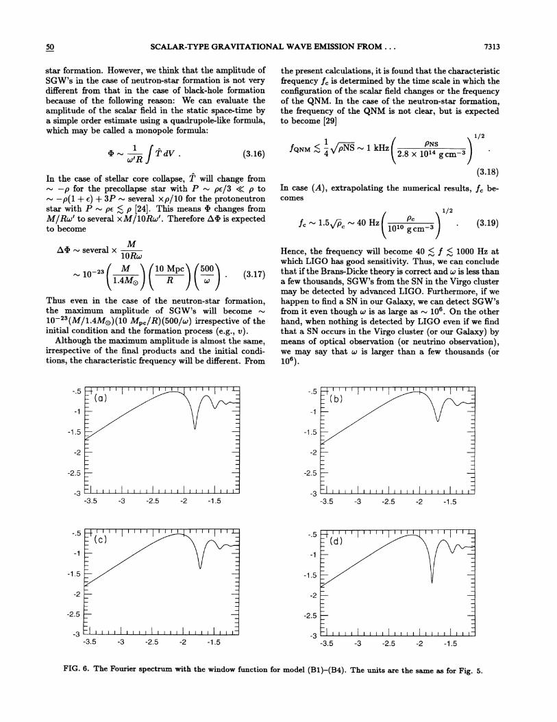
Hence, the frequency will become 40 & f & 1000 Hz atwhich LIGO has good sensitivity. Thus, we can concludethat if the Brans-Dicke theory is correct and u is less thana few thousands, SGW's from the SN in the Virgo clustermay be detected by advanced LIGO. Furthermore, if wehappen to find a SN in our Galaxy, we can detect SGW'sfrom it even though ur is as large as 10 . On the otherhand, when nothing is detected by LIGO even if we findthat a SN occurs in the Virgo cluster (or our Galaxy) bymeans of optical observation (or neutrino observation),we may say that u is larger than a few thousands (or10 ).

the present calculations, it is found that the characteristicfrequency f, is determined by the time scale in which theconfiguration of the scalar field changes or the frequencyof the QNM. In the case of the neutron-star formation,the frequency of the QNM is not clear, but is expectedto become [29]

X/2

fqNM & —gpNS 1 kHzi~2.8 x 10~4 gem s

~

(3.18)

In case (A), extrapolating the numerical results, f, be-comes

-5 i i i

[i 1 i ~l i i i

-1 5 -1.5

-2:-2.5—

3-3.5 -3 -2.5 -2 -1.5

2:-2.5—

3-3.5 -3 -2.5 -2 -1.5

I I I I I I I I I I

-5 i i ii

i i i i

i

i i i i i i i i i

Ii i -.5

-1.5 -1.5

-2.5—-3

-3.5 -2.5 -2 -1.5I I I I I I I I I I I I I I I I I

-2.5—

3 I i i i i I i i i i

-3.5 -3 -2.5I I I I I I I I I I

-2 -1.5

FIG. 6. The Fourier spectrum with the window function for model (81)—(84). The units are the same as for Fig. 5.

7314 MASARU SHIBATA, KENICHI NAKAO, AND TAKASHI NAKAMURA

C. Detection of SG%V's

In the above, our discussion assumed that the laserinterferometric detector has the ability to detect SGW's,whereas it is a nontrivial problem. Thus, we here brie8yshow it as possible in reality.

In the wave zone composed of SGW's, the line elementcan be written as u=t —z and v =t+z. {3.26)

the mirror within the z-y plane does not occur even ifthe SGW 4(t-z) arrives at the mirror.

On the other hand, the SGW causes a nontrivial mo-tion of the mirror in the z direction. Here we intro-duce the retarded and advanced time coordinates (u, v)to make the equations simple:

ds = (1+4)(—dt +de +dy +dz ) . (3.20) From Eqs. (3.21) and (3.23), we obtain

d dt 1 Bg(1+ 4)d7 dr 2 1+4 (3.21)

This is the conformally Sat space-time in which the nullstructure is completely the same as the Minkowski space-time, so that the laser (light) does not change their passand the phase shift does not occur, by SGW's, as long asthe laser goes along a null geodesic. Hence, it seems to beimpossible to detect SGW's by the laser interferometricdetector. However, this is not the case. We should notethat the laser is reflected by the mirror again and againin the detector and the pass of the laser changes. If themiiTor is not in6uenced by SGW's and rests, there is nosignal in the detector, since the laser goes along the nullgeodesic efFectively. However, if the mirror is perturbedby SGW's, the phase difference is caused and the inter-ferometric detector can detect SGW's. As will be shownbelow, in reality it happens.

When the SGW comes from a very distant source, itcan be approximated as a plane wave at the detector.Hence, we assnme that the SGW 4 is a function of tz and, in this case, the geodesic equation of a mirrorbecomes

d ~ du I (9„4u[1+4( )l-d~ ( d~) 1+4(u)

(3.27)

Then we get

dQ

d7 1+ C (u)(3.28)

dv 1

d7 a(3.29)

and

7 = av+b, (3.30)

where b is an integration constant, which correspondsmerely to the advanced time coordinate translation, and,hence, without loss of generality we will take it to bezero. In order to see the meaning of the other integrationconstant a, we write down the equation for z from Eqs.(3.28) and (3.29) as

where a is an integration constant. From Eqs. (3.24) and(3.28), we find

dz dy—(1+4)—= 0 = —(1+4)—d7. d7. d~ d7.

(3.22)dz 1 f a'1—d7' 2a

I 1+4)(3.31)

d dz 18(1+4)d~ d~ 2 1+4 (3.23)

Before the SGW arrives at the mirror, i.e., 4 = 0, theabove equation becomes

where 7 is the proper time of the mirror and in order toderive the above equations we have used the relation

dz 1—= —(1 —a).d'T a

(3.32)

(dt ~ ~dxl Idyl ~dz~ 1

d~) I d~) I d~) ) d~) 1+(3.24)

This is just the initial velocity of the mirror, so we willchoose a = 1 because the mirror initially rests.

Now we can find the motion of the mirror in the zdirection by integrating Eq. (3.28) as

Equation (3.22) is immediately integrated and we obtain

dx(1+4)—= P = const,d~

(1 + 4') —= PII = constdyd~

(3.25)

Since we ass»~e that the mirror is at rest initially, Pand Pz should vanish. This means that the motion of

z = —,'(z —z;) = -', J(1+O(u))dz —z~

t—a= zp + 2 4 (u)du, (3.33)

where zo is the initial location of the mirror and we haveused the fact 7 = v. Then assnming 4 « 1, the displace-ment of the mirror in the z direction is given by

50 SCALAR-TYPE GRAVITATIONAL WAVE EMISSION FROM. . . 7315

t—sp —Az4z=z —zp ——

21 O(u) du

B,.&

q(r) = Kg+ — —+r=0. (4 1)

4(u)du . (3.34) In n»merical simulations, we determine the location ofthe apparent horizon, r = r;, from the condition

[n mq —n m2] = sin8, /1 —sin2y, , (3.35)

where mq and m2 are the directions of the two armsof the detector and are assumed to be mq ——(1,0, 0)and m2 ——(0, 1,0). n = (8„((s,) describes the incomingdirection of the wave to the detector [2]. Equation (3.35)means that if one of the arms of the detector agrees withthe incoming direction of SGW, the sensitivity becomesmaxim~~m. In this case, the phase difference Ag at themaximum displacement of the mirror is given by

2' Az 04(u) du,

A 2(3.36)

As shown above, the mirrors move only in the propaga-tion direction z of the waves. This means that in thecase that the detector lies on the z-y plane, the sensi-tivity of the detector is zero because the arm length ofthe laser interferometer does not change even if the SGWcomes. However, the sensitivity of the detector to SGW'sis not zero in the other cases because the arm length ofthe detector must be changed. The change of arm lengthmeans that the pass of the laser is also changed, so thatthe laser interferometer can measure the change, i.e., de-tect SGW's. (This also explains why the noise level of thelaser interferometer to + and x modes of gravitationalwaves is roughly the same as that of the scalar mode. )

The antenna pattern of the laser interferometric detec-tor is proportional to

(4.2)

In all the models, we find that the apparent horizon wasformed and these results strongly suggest that the blackhole was formed. To make sure that those are the ap-parent horizon around the Schwarzschild black holes, wealso calculate their area (S) from

S/M = 4mB r (4.3)

We find that in all calculations S/M2 becomes & 16'',where 16m is the area of the event horizon of theSchwarzschild black hole.

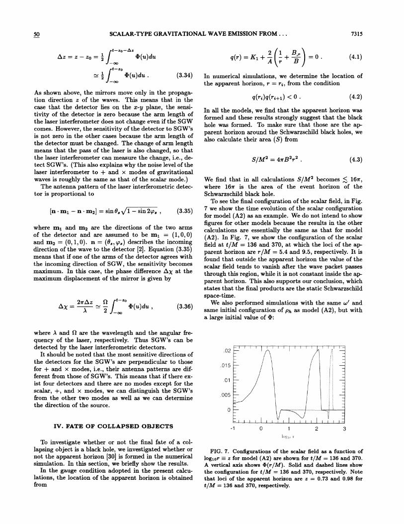
To see the final configuration of the scalar field, in Fig.7 we show the time evolution of the scalar configurationfor model (A2) as an example. We do not intend to showfigures for other models because the results in the othercalculations are essentially the same as that for model(A2). In Fig. 7, we show the configuration of the scalarfield at t/M = 136 and 370, at which the loci of the ap-parent horizon are r/M = 5.4 and 9.5, respectively. It isfound that outside the apparent horizon the value of thescalar field tends to vanish after the wave packet passesthrough this region, while it is not constant inside the ap-parent horizon. This also supports our conclusion, whichstates that the final products are the static Schwarzschildspace-time.

We also performed simulations with the same ~' andsame initial configuration of p~ as model (A2), but witha large initial value of 4:

where A and 0 are the wavelength and the angular fre-quency of the laser, respectively. Thus SGW's can bedetected by the laser interferometric detectors.

It should be noted that the most sensitive directions ofthe detectors for the SGW's are perpendicular to thosefor + and x modes, i.e., their antenna patterns are dif-ferent from those of SGW's. This means that if there ex-ist four detectors and there are no modes except for thescalar, +, and x modes, we can distinguish the SGW'sRom the other two modes as well as we can determinethe direction of the source.

.02

.015

.01

.005

IIII I

I II

I

IIII III II II III II iI II II II Ii I

I II II II 1

I II II II I

I II II I

II II II I

IV. FATE OF COLLAPSED OBJECTSI I I I I I I I I I I I

To investigate whether or not the final fate of a col-lapsing object is a black hole, we investigated whether ornot the apparent horizon [30] is formed in the numericalsimulation. In this section, we briefiy show the results.

In the gauge condition adopted in the present calcu-lations, the location of the apparent horizon is obtained&om

FIG. 7. ConSgurations of the scalar Seld as a function oflogqor—:z for model (A2) are shown for t/M = 136 and 370.A vertical axis shows 4(r/M). Solid and dashed lines showthe configuration for t/M = 136 and 370, respectively. Notethat loci of the apparent horizon are z = 0.73 and 0.98 fort/M = 136 and 370, respectively.

7316 MASARU SHIBATA, KENICHI NAKAO, AND TAKASHI NAKAMURA 50

0—

0

I

I&

IIiI

I

I

jI

I I 1

I II

1

III

II (I (

I )o1(

500 M 10 Mp,

( u) ) (10MO) 4R )

(5.2)

Using the results of the present calculation, we canroughly estimate that in the realistic gravitational col-lapse and the subsequent neutron star formation, f, be-comes

While the characteristic frequency f depends either onthe QNM of the black hole, f 200—400M/10Mci Hz,or on the initial condition, in which f, is approximatelyproportional to +p, where p, is the density when thecollapse to black hole begins, the characteristic amplitudebecomes

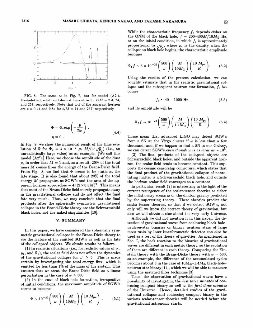
FIG. 8. The same as in Fig. 7, but for model (A2').Dash-dotted, solid, and dashed lines show for t/M = 2.3, 74,and 257, respectively. Note that loci of the apparent horizonare z = 0.44 and 0.84 for t/M = 74 and 257, respectively.

f, 40 —1000 Hz,

and its amplitude will be

(5.3)

4 = 4,exp~— yl„&5001 & M 'l I'10M„&

4'f f 10I

ur ) (1.4MO) ( 8 )(5.4)

g=0.(4.4)

In Fig. 8, we show the numerical result of the time evo-lution of 4 for 4, = 4 x 10 » M/(ur'~yi) (i.e., anunrealistically large value) as an example. [We call thismodel (A2').] Here, we choose the amplitude of the dust

p, in order that M = 1 and, as a result, 20% of the totalmass M comes &om the energy of the Brans-Dicke field.From Fig. 8, we find that 4 seems to be static at thelate stage. It is also found that about 20% of the totalenergy M propagates as SGW's and the area of the ap-parent horizon approaches 4m(2 x 0.8M)2. This meansthat most of the Brans-Dicke field merely propagate awayin the gravitational collapse and do not afFect the finalfate very much. Thus, we may conclude that the finalproducts after the spherically symmetric gravitationalcollapse in the Brand-Dicke theory are the Schwarzschildblack holes, not the naked singularities [19].

V. SUMMARY

(5001 ( M & &10M„I4 10~10MO) ~

R (5.1)

In this paper, we have considered the spherically sym-metric gravitational collapse in the Brans-Dicke theory tosee the feature of the emitted SGW's as mell as the fateof the collapsed objects. We obtain results as follows.

(1) In realistic situations (i.e. , for realistic values of p„yi, and 4,), the scalar field does not affect the dynamicsof the gravitational collapse for u' & 5. This is madecertain by investigating the total-energy Bux, which isemitted for less than 1% of the mass of the system. Thisensures that we treat the Brans-Dicke field as a linearperturbation in the case of u & 500.

(2) In the case of black-hole formation, irrespectiveof initial conditions, the maximum amplitude of SGW'sseems to become

These mean that advanced I IGO may detect SGW's&om a SN at the Virgo cluster if a is less than a fewthousand, and, if we happen to find a SN in our Galaxy,we can detect SGW's even though ur is as targe as 10s.

(3) The final products of the collapsed objects areSchwarzschild black holes, and outside the apparent hori-zon, the scalar field tends to become constant. This sup-ports the cosmic censorship conjecture, which states thatthe final product of the gravitational collapse of nonro-tating matter is a Schwarzschild black hole, and outisdethe horizon scalar field converges to a constant.

In particular, result (2) is interesting in the light of thecurrent resurgence of the scalar-tensor theories as eitherthe infiationary scenario or the dilaton gravity predictedby the superstring theory. These theories predict thescalar-tensor theories, so that if we detect SGW's, notonly will we know the correct theory of gravitation, butalso we will obtain a clue about the very early Universe.

Although we did not mention it in this paper, the de-tection of gravitational waves &om coalescing black-hole—neutron-star binaries or binary neutron stars of largemass ratio by laser interferometric detector can also beused as a test of the theory of gravities. As mentioned inSec. I, the back reaction to the binaries of gravitationalwaves are difFerent in each metric theory, so the evolutionof them are difFerent in each theory. Comparing the Ein-stein theory with the Brans-Dicke theory with ~ = 500,as an example, the difference of the accumulated cyclesbecomes about 3 in the case of 10MO —1.4MO black-hole—neutron-star binary [14],which we will be able to measureusing the matched filter technique [3].

Thus, the observation of gravitational waves have apossibility of investigating the last three minutes of coa-lescing compact binary as well as the first thee minutesof the Universe. Hence, detailed studies of the gravi-tational collapse and coalescing compact binary in thevarious scalar-tensor theories will be needed before thegravitational astronomy starts.

50 SCALAR-TYPE GRAVITATIONAL WAVE EMISSION FROM. . . 7317

ACKNOW LEDC MENTS

We thank H. Ishihara, M. Sasaski, H. Tagoshi, andT. Tanya for use&8 comments and discussions. K. N.

is also grateful to H. Sato for his encouragement. Thiswork eras partly supported by a Grant-in-Aid Scienti6cResearch on Priority Area of the Ministry of Education,Science and Culture, No. 04234104.

[1] R. E. Vogt, in Sizth Marcel Grossrnann Meeting on Generul Relativity, Proceedings, Kyoto, Japan, 1991, editedby H. Sato and T. Nakamura (World ScientiSc, Sin-gapore, 1991), p. 244; A. Abramovici et al. , Science25B, 325 (1992); K. S. Thorne, in Proceedings of theEighth Nishinomiya Symposium on Relativistic Astro-physics, Nishinomiya, Japan, 1993, edited by M. Sasaki(Universal Academy, Nishinomiya, 1993).

[2] K. S. Thorne, in 800 Years of Gravitation, edited by S.W. Hawking and W. Israel (Cambridge University Press,Cambridge, England, 1987).

[3] C. Cutler et al. , Phys. Rev. Lett. 70, 2984 (1993).[4] L. E.Kidder, C. M. Will, and A. G. Wiseman, Phys. Rev.

D 47, R4183 (1993);M. Shibata, ibid 48, .663 (1993).[5) C. Cutler and E. E. Flanagan, Phys. Rev. D 49, 2658

(1994).[6] M. Shibata, Prog. Theor. Phys. 90, 595 (1993); T. A.

Apostolatos, C. Cutler, G. J. Sussman, and K. S. Thorne(unpublished).

[7) A. Krolak and B. F. Schutz, Gen. Relativ. Gravit. 19,1163 (1987).

[8] D. Markovic, Phys. Rev. D 48, 4738 (1993).[9) For example, R. Narayan, B. Paczynski, and T. Piran,

Astrophys. J. $95, L83 (1992);T. Nakamura et aL, Prog.Theor. Phys. 8'7, 879 (1992), and references therein.

[10) C. M. Will, Theory and Ezperirnent in GravitationalPhysics (Cambridge University Press, Cambridge, Eng-land, 1992), and references therein.

[ll] J. H. Taylor and J. M. Weisberg, Astrophys. J. $45, 434(1989); T. Damour and J. H. Taylor, Phys. Rev. D 45,1840 (1992).

[12) T. Damour and A. M. Polyakov, report (unpublished).[13] C. Brans and R. H. Dicke, Phys. Rev. 124, 925 (1961).

[14] C. M. Will and H. W. Zaglauer, Astrophys. J. $46, 366(1989).

[15] D. M. Eardley, D. L. Lee, and A. P. Lightman, Phys.Rev. D 8, 3308 (1973).

[16] D. L. Lee, Phys. Rev. D 10, 2374 (1974).[17] R. Monchmeyer et al. , Astron. Astrophys 2.5B, 417

(1991);L. S.Finn, Ann. N. Y. Acad. Sci. 6$1, 156 (1991).[18] H. W. Zaglauer, Astrophys J. $. 9$, 685 (1992).[19] S. W. Hawking, Commun. Math. Phys. 25, 167 (1972);

Y. Suzuki and M. Yoshimura, Phys. Rev. D 4S, 2549(1991).

[20] R. H. Dicke, Phys. Rev. 125, 2163 (1962).[21] W. H. Press et al. , Numerical Recipes (Cambridge Uni-

versity Press, Cambridge, England, 1989).[22] L. I. Petrich, S. L. Shaprio, and S. A. Teukolsky, Phys.

Rev. D $1, 2459 (1985).[23) D. M. Eardley and L. Smarr, Phys. Rev. D 19, 2239

(1979).[24] S. L. Shapiro and S. A. Teukolsky, Black Holes, White

Dwar fa and Neutron Stars (Wiley-Interscience, NewYork, 1983).

[25] T. Matsuda and H. Nariai, Prog. Theor. Phys. 49, 1195(1973).

[26) T. Nakamura, K. Oohara, and Y. Kojima, Prog. Theor.Phys. Suppl. 99, 110 (1987).

[27] B. F. Schutz and C. M. Will, Astrophys. J. 291, L33(1985).

[28] R. F. Stark and T. Piran, Phys. Rev. Lett. 55, 891 (1985).[29] L. Lindblom and S. L. Detweiler, Astrophys. J. Suppl.

5$, 73 (1983).[30] R. M. Wald, General Relativity (University of Chicago

Press, Chicago, 1984).