Scalar-tensor cosmologies with a potential in the general
10
Journal of Physics: Conference Series OPEN ACCESS Scalar-tensor cosmologies with a potential in the general relativity limit To cite this article: Laur Järv et al 2011 J. Phys.: Conf. Ser. 283 012017 View the article online for updates and enhancements. You may also like Beyond the Friedmann—Lemaître—Robertson—Walk er Big Bang Singularity Cristi Stoica - Is Cosmology Solved? An Astrophysical Cosmologist's Viewpoint P. J. E. Peebles - Past extendibility and initial singularity in Friedmann-Lemaître-Robertson-Walker and Bianchi I spacetimes Kimihiro Nomura and Daisuke Yoshida - Recent citations Transformation properties and general relativity regime in scalar–tensor theories Laur Järv et al - Scalar-tensor cosmological models converging to general relativity: potential dominated and matter dominated cases Margus Saal et al - Evolution of homogeneous and isotropic scalar-tensor cosmological models Piret Kuusk et al - This content was downloaded from IP address 192.140.87.193 on 04/01/2022 at 10:18
Transcript of Scalar-tensor cosmologies with a potential in the general

Journal of Physics Conference Series
OPEN ACCESS
Scalar-tensor cosmologies with a potential in thegeneral relativity limitTo cite this article Laur Jaumlrv et al 2011 J Phys Conf Ser 283 012017
View the article online for updates and enhancements
You may also likeBeyond theFriedmannmdashLemaicirctremdashRobertsonmdashWalker Big Bang SingularityCristi Stoica
-
Is Cosmology Solved An AstrophysicalCosmologists ViewpointP J E Peebles
-
Past extendibility and initial singularity inFriedmann-Lemaicirctre-Robertson-Walkerand Bianchi I spacetimesKimihiro Nomura and Daisuke Yoshida
-
Recent citationsTransformation properties and generalrelativity regime in scalarndashtensor theoriesLaur Jaumlrv et al
-
Scalar-tensor cosmological modelsconverging to general relativity potentialdominated and matter dominated casesMargus Saal et al
-
Evolution of homogeneous and isotropicscalar-tensor cosmological modelsPiret Kuusk et al
-
This content was downloaded from IP address 19214087193 on 04012022 at 1018
Scalar-tensor cosmologies with a potential in the
general relativity limit
Laur Jarv1 Piret Kuusk1 and Margus Saal2
1 Institute of Physics University of Tartu Riia 142 EE-51014 Tartu Estonia2 Tartu Observatory EE-61602 Toravere Tartumaa Estonia
E-mail laurjarvutee
Abstract We consider Friedmann-Lemaıtre-Robertson-Walker flat cosmological models inthe framework of general Jordan frame scalar-tensor theories of gravity with arbitrary couplingfunctions in the era when the energy density of the scalar potential dominates over the energydensity of ordinary matter To study the regime suggested by the local weak field tests (ie closeto the so-called limit of general relativity) we propose a nonlinear approximation scheme solvefor the phase trajectories and provide a complete classification of possible solutions We arguethat the topology of phase trajectories in the nonlinear approximation is representative of thoseof the full system and thus can tell for which scalar-tensor models general relativity functionsas an attractor To the classes of models which asymptotically approach general relativity wegive the solutions also in cosmological time and conclude with some observational implications
1 Introduction
One of the most outstanding problems for contemporary physics is how to explain the dynamicsbehind the current accelerated expansion of the universe A plethora of various approacheshave been proposed most of which can be subsumed under the categories of dark energy(extraordinary matter) or dark gravity (modifications to Einsteinrsquos general relativity) As newastrophysical and cosmological precision data is continuously becoming available it remainsa cumbersome task to systematically sift out the models which can meet all observationalrequirements What one would like to have are reliable model independent tools for testinggravity at large scales perhaps something akin to the parametrized post-Newtonian (PPN)formalism for weak fields
While there has been some progress in designing such tools (the post-Friedmannianformalism) here we would like to introduce a bit more modest approach in scope yet witha congruent aim First we note that many proposed modified gravity theories can be cast inthe form of scalar-tensor gravity (STG) ndash higher dimensional theories braneworld models f(R)type gravities varying speed of light theories etc Second wide classes of STG cosmologiesdynamically converge to the limit of general relativity favored by local weak field experimentsthe so-called ldquoattractor mechanismrdquo [1] Therefore we can use generic STG as a template orparadigm which implicitly incorporates many different theories in order to confront them withvarious observations and see how good they are in comparison with each other In principle thisshould provide an instrument of selection within the zoo of modified gravities
In the present paper we review our recent work towards this direction [2 3 4 5] Aftersetting the notation and describing the local weak field constraints in Section 2 we write the
Recent Developments in Gravity (NEB XIV) IOP PublishingJournal of Physics Conference Series 283 (2011) 012017 doi1010881742-65962831012017
Published under licence by IOP Publishing Ltd 1
scalar-tensor cosmology as a dynamical system and briefly outline the features of the phasespace in Section 3 followed by the discussion of the fixed points in Section 4 The fixed pointcorresponding to limit of general relativity needs a more careful consideration facilitated by theapproximation scheme of Section 5 This leads to approximate equations which are used tofind and classify the phase portraits in Section 6 and to find the solutions in time in Section 7Finally Section 8 provides a brief summary and outlook
2 Scalar-tensor gravity and local weak field constraints
We start with a generic Jordan frame STG using the ldquoBrans-Dickerdquo parametrization
S =1
2κ2
int
d4xradicminusg
[
ΨR[gmicroν ] minus ω(Ψ)
ΨnablaρΨnablaρΨ minus 2κ2V (Ψ)
]
+ Sm (1)
In fact the action above describes a family of theories each pair of the functions ω(Ψ) and V (Ψ)specifies a particular STG The non-minimal coupling between curvature and the scalar field Ψ
means variable gravitational ldquoconstantrdquo 8πG = κ2
Ψ and it makes sense to assume 0 lt Ψ lt infinTo ensure that the energy density of the scalar field is positive one also needs 2ω(Ψ) + 3 ge 0and V (Ψ) ge 0 The term Sm gives the usual matter part of the action
Local weak field experiments (eg observations in the Solar System) reckoned in terms of thePPN formalism impose rather severe constraints on the theory If V (Ψ) can be neglected then
8πG =κ2
Ψ
2ω + 4
2ω + 3 (2)
β minus 1 =κ2
G
dωdΨ
(2ω + 3)2(2ω + 4) 10minus4 (3)
γ minus 1 = minus 1
ω + 2 10minus5 (4)
G
G= minusΨ
2ω + 3
2ω + 4
(
G +2 dω
dΨ
(2ω + 3)2
)
10minus13 yrminus1 (5)
These constraints are satisfied by STG in the ldquoNordtvedt limitrdquo [6]
1
2ω + 3rarr 0
dωdΨ
(2ω + 3)3rarr 0 (6)
in which case the predictions of STG and GR coincide and we may call (6) also ldquothe limit ofgeneral relativityrdquo (If V (Ψ) gives a contribution then the PPN parameters get a correction[7 8])
Recent Developments in Gravity (NEB XIV) IOP PublishingJournal of Physics Conference Series 283 (2011) 012017 doi1010881742-65962831012017
2
3 Scalar-tensor cosmology as a dynamical system
The field equations for flat (k = 0) Fridmann-Lemaıtre-Robertson-Walker spacetime filled withbarotropic matter fluid p = wρ read
H2 = minusHΨ
Ψ+
1
6
Ψ2
Ψ2ω(Ψ) +
κ2
3
ρ
Ψ+
κ2
3
V (Ψ)
Ψ (7)
2H + 3H2 = minus2HΨ
Ψminus 1
2
Ψ2
Ψ2ω(Ψ) minus Ψ
Ψminus κ2
Ψwρ +
κ2
ΨV (Ψ) (8)
Ψ = minus3HΨ minus 1
2ω(Ψ) + 3
dω(Ψ)
dΨΨ2 +
κ2
2ω(Ψ) + 3(1 minus 3w) ρ
+2κ2
2ω(Ψ) + 3
[
2V (Ψ) minus ΨdV (Ψ)
dΨ
]
(9)
ρ = minus3H (w + 1) ρ (10)
where H is the Hubble parameter Denoting Π = Ψ the equations (7)-(10) can be rewritten asa dynamical system
Ψ = Π (11)
Π = minus 1
2ω(Ψ) + 3
[
dω(Ψ)
dΨΠ2 minus κ2 (1 minus 3w) ρ
+2κ2
(
dV (Ψ)
dΨΨ minus 2V (Ψ)
)
]
minus 3HΠ (12)
H =1
2Ψ(2ω(Ψ) + 3)
[
dω(Ψ)
dΨΠ2 minus κ2 (1 minus 3w) ρ
+2κ2
(
dV (Ψ)
dΨΨ minus 2V (Ψ)
)
]
minus 1
2Ψ
[
6H2Ψ + 2HΠ minus κ2(1 minus w)ρ minus 2κ2V (Ψ)]
(13)
ρ = minus3H(1 + w)ρ (14)
while the vector (Ψ Π H ρ) gives a tangent to the trajectories (solutions) in the phase spaceΨΠH ρ The trajectories lie on the 3-surface
H = minus Π
2Ψplusmnradic
(2ω(Ψ) + 3)Π2
12Ψ2+
κ2(ρ + V (Ψ))
3Ψ (15)
By carefully inspecting Eq (11)-(14) we can elicit the following generic information about theboundaries in the phase space [2 3]
bull |H| rarr infin |ρ| rarr infin or |Ψ| rarr infin imply a spacetime curvature singularity
bull Ψ rarr 0 generally also leads to a singularity (solutions can not slip from ldquoattractiverdquo toldquorepulsiverdquo gravity)
bull Ψ rarr infin is not a singularity but gravitational ldquoconstantrdquo κ2
Ψ vanishes
bull V rarr infin or 2ω + 3 rarr 0 is again a singularity solutions can not safely pass to the regionwhere Ψ turns to a ghost (2ω + 3 lt 0)
bull 12ω+3 rarr 0 turns out to be a singularity as well unless Ψ = Π rarr 0
Recent Developments in Gravity (NEB XIV) IOP PublishingJournal of Physics Conference Series 283 (2011) 012017 doi1010881742-65962831012017
3
4 Fixed points
If on cosmological scales the potential dominates over matter density (V 6equiv 0 ρ equiv 0) we caneliminate H using (15) and obtain a 2-dimensional system
Ψ = Π (16)
Π =
(
3
2Ψminus 1
2ω(Ψ) + 3
dω
dΨ
)
Π2 +2κ2
2ω(Ψ) + 3
(
2V (Ψ) minus ΨdV
dΨ
)
∓ 1
2Ψ
radic
3(2ω(Ψ) + 3)Π2 + 12κ2ΨV (Ψ) Π (17)
The fixed points (Ψ = 0 Π = 0) are of two types given by [2]
Ψbull dV
dΨ
∣
∣
∣
Ψbull
Ψbull minus 2V (Ψbull) = 0 (18)
Ψ⋆ 1
2ω(Ψ⋆) + 3= 0
1
(2ω(Ψ⋆) + 3)2dω
dΨ
∣
∣
∣
Ψ=Ψ⋆
6= 0 (19)
(Strictly speaking the latter case assumes (2ω(Ψ⋆) + 3)Π2⋆ = 0 see below Section 5 for an
improved approach) The properties of the fixed points (stable unstable) and the form of thesolutions around the fixed points are determined by the eigenvalues and these by the values
ω(Ψbull⋆)dωdΨ |Ψbull⋆
V (Ψbull⋆)dVdΨ |Ψbull⋆
d2VdΨ2 |Ψbull⋆
Notice that Ψ⋆ is compatible with the ldquolimit ofgeneral relativityrdquo ie the local weak field experiments (the matter density in the Solar Systemis still much higher than the energy density of the potential even if on the cosmological scales thepotential may dominate) On the other hand the Ψbull point is generally not in accord with theweak field observations although in some special situations it may perhaps be possible salvageit by taking into account the contribution of the potential to the PPN paramaters
If matter density dominates over potential (ρ 6equiv 0 V equiv 0) we can use a new time variable
dp equiv∣
∣
∣H + Ψ
2Ψ
∣
∣
∣dt to eliminate H and obtain
Ψprime = Υ (20)
Υprime = plusmn2ω(Ψ) + 3
8Ψ2Υ3 +
6ω(Ψ) + 9 minus 4Ψdω(Ψ)dΨ
4Ψ(2ω(Ψ) + 3)Υ2 ∓ 3
2Υ +
3Ψ
2ω(Ψ) + 3 (21)
The fixed point (Ψprime = 0Υprime = 0) in p-time corresponds to a fixed point (Ψ = 0 Π = 0) in t-timeand is given by [2]
Ψ⋆ 1
2ω(Ψ⋆) + 3= 0
1
(2ω(Ψ⋆) + 3)2dω
dΨ
∣
∣
∣
Ψ=Ψ⋆
6= 0 (22)
Again it is good to see that the fixed point turns out to be compatible with the ldquolimit of generalrelativityrdquo
5 Approximation scheme for the ldquolimit of general relativityrdquo
In the GR limit (Ψ⋆Π⋆) ie (a) 12ω(Ψ)+3 rarr 0 (b) Ψ equiv Π rarr 0 the equations contain a 0
0
type indeterminacy (like yx
at the origin) thus demanding a more careful analysis Let us focusaround the vicinity of this point Ψ = Ψ⋆ + x Π = Π⋆ + y = y and expand in series (x and y
being first order small)
1
2ω(Ψ) + 3=
1
2ω(Ψ⋆) + 3+ A⋆x + asymp A⋆x (23)
(2ω(Ψ) + 3)Π2 =y2
0 + A⋆x + =
y2
A⋆x(1 + O(x)) asymp y2
A⋆x (24)
Recent Developments in Gravity (NEB XIV) IOP PublishingJournal of Physics Conference Series 283 (2011) 012017 doi1010881742-65962831012017
4
where (c) A⋆ equiv ddΨ
(
12ω(Ψ)+3
)∣
∣
∣
Ψ⋆
6= 0 ja (d) 12ω(Ψ)+3 is differentiable at Ψ⋆ In the following we
will focus on the case when the matter density can be neglected in favor of the potential (ietake V 6equiv 0 ρ equiv 0 ) Keeping only the terms which are of first order in x and y the dynamicalsystem (16) (17) becomes [4]
x = y (25)
y =y2
2xminus C1 y + C2 x (26)
where the constants
C1 equiv plusmnradic
3κ2V (Ψ⋆)
Ψ⋆
C2 equiv 2κ2A⋆
(
2V (Ψ) minus dV (Ψ)
dΨΨ
)
∣
∣
∣
Ψ⋆
(27)
encode the behavior of the functions ω and V near the GR point In a similar manner the PPN
parameters (3) (4) and GG
(5) are approximated by
β minus 1 = minus1
2A2
⋆Ψ⋆x (28)
γ minus 1 = minus2A⋆x (29)
G
G= minus1 minus A⋆Ψ⋆
Ψ⋆
x (30)
Via the Friedmann equation (15) we can also express H(x(t)) H(x(t)) and get the equation ofstate parameter as
w = minus1 minus 2H
3H2= minus1 +
1
C21Ψ⋆
[
3
2
(
1 +1
Ψ⋆A⋆
)
x2
xminus 4C1x + 3C2x
]
(31)
6 Phase space trajectories
The phase trajectories for the nonlinear approximate system (25) (26) are determined by theequation
dy
dx=
y
2xminus C1 +
x
yC2 (32)
Its solutions depend on the sign of C21 + 2C2 equiv C [4]
|x|K =
∣
∣
∣
∣
1
2y2 + C1yx minus C2x
2
∣
∣
∣
∣
exp(minusC1f(u)) u equiv y
x (33)
f(u) =1radicC
ln
∣
∣
∣
∣
∣
u + C1 minusradic
C
u + C1 +radic
C
∣
∣
∣
∣
∣
if C gt 0
= minus 2
u + C1if C = 0
=2
radic
|C|
(
arctanu + C1radic
|C|+ nπ
)
if C lt 0 (34)
The phase portraits which emerge for the various values of the constants are classified in Table1 and depicted on Figure 1 As the approximate system is non-linear the phase portraits split
Recent Developments in Gravity (NEB XIV) IOP PublishingJournal of Physics Conference Series 283 (2011) 012017 doi1010881742-65962831012017
5
Table 1 The topology of trajectories for the approximate nonlinear system (32)
No Parameters Topology of trajectories
C gt 0 1a C1 gt 0 C2 gt 0 2 hyperb 2 st amp 2 unst parab sectors
1b C1 gt 0 C2 = 0 1 stable amp 1 unstable parabolic sector
2 stable sectors of degenerate fixed points
1c C1 gt 0 minusC2
1
2 lt C2 lt 0 2 elliptic 4 stable parabolic sectors
1d C1 = 0 C2 gt 0 2 hyperb 2 st amp 2 unst parab sectors
1e C1 lt 0 C2 gt 0 2 hyperb 2 st amp 2 unst parab sectors
1f C1 lt 0 C2 = 0 1 stable amp 1 unstable parabolic sector
2 unst sectors of degenerate fixed points
1g C1 lt 0 minusC2
1
2 lt C2 lt 0 2 elliptic 4 unstable parabolic sectors
C = 0 2a C1 gt 0 C2 = minusC2
1
2 2 elliptic 2 stable parabolic sectors
2b C1 = 0 C2 = 0 2 stable amp 2 unstable parabolic sectors
2c C1 lt 0 C2 = minusC2
1
2 2 elliptic 2 unstable parabolic sectors
C lt 0 3a C1 gt 0 C2 lt minusC2
1
2 2 elliptic sectors
3b C1 = 0 C2 lt 0 2 elliptic sectors
3c C1 lt 0 C2 lt minusC2
1
2 2 elliptic sectors
into sectors which can be hyperbolic elliptic or parabolic stable or unstable Typically thereare many trajectories passing through the GR point either once or multiple times
By comparing the tangents of the trajectories in full system (16)-(17) with the ones of thenonlinear approximate system (25)-(26) we can argue [4] that the topology of trajectories inthe nonlinear approximation is representative of those of the full system Therefore one shouldtake the results of the nonlinear approximation seriously In the end the classification of thephase portraits reveals that only if C1 gt 0 and C2 lt 0 ie
d
dΨ
(
1
2ω(Ψ) + 3
)
∣
∣
∣
∣
∣
Ψ⋆
(
2V (Ψ) minus dV (Ψ)
dΨΨ
)
∣
∣
∣
∣
∣
Ψ⋆
lt 0 (35)
does the GR point function as an asymptotic attractor for the flow of all trajectories in thevicinity
Recent Developments in Gravity (NEB XIV) IOP PublishingJournal of Physics Conference Series 283 (2011) 012017 doi1010881742-65962831012017
6
1a (1d) 1b 1c
1e (1d) 1f 1g
2a 2b 2c
3a 3b 3c
Figure 1 Phase portraits of the nonlinear approximation (32) near the GR point (Axesx = Ψ minus Ψ⋆ horizontal and y = Ψ vertical)
Recent Developments in Gravity (NEB XIV) IOP PublishingJournal of Physics Conference Series 283 (2011) 012017 doi1010881742-65962831012017
7
7 Time evolution
The approximate system (25)-(26) can be also combined into a second order equation
x + C1x minus C2x =x2
2x (36)
yielding solutions in terms of the cosmological time [5]
plusmnx = eminusC1t[
M1e1
2tradic
C minus M2eminus 1
2tradic
C]2
if C gt 0 (37)
= eminusC1t[
e1
2C1t1t minus M2
]2 if C = 0 (38)
= eminusC1t
[
N1 sin(1
2tradic
|C|) minus N2 cos(1
2tradic
|C|)]2
if C lt 0 (39)
where M1M2 t1N1N2 are constants of integration (determined by the initial conditions) Inparticular the behavior of solutions which approach general relativity can be classified undertwo characteristic types (i) exponential or linear exponential convergence and (ii) dampedoscillations around general relativity
Given the solutions above one can now plug x(t) into the expressions for the PPN paramaters
(28) (29) or GG
(30) or w (31) to find how they should evolve in time The solutions for whichGR is an attractor eventually converge to de Sitter of course But as they do it some ofthem have oscillating some monotonically evolving w There are solutions which do not crossthe phantom divide (w = minus1) solutions which cross it only once and solutions which cross itperiodically The particular behavior is determined by the constants C1 C2 and A⋆ (and tocertain extent also by the initial conditions)
8 Summary and outlook
We have found and characterized the fixed points of STG cosmology in the case when potentialdominates over cosmological matter density In particular we have also found the general analyticform of solutions around the fixed points This can be applied to cosmological expansion ourresults inform whether the solutions of any particular theory have oscillating phantom crossingetc behavior
The analysis in the case of matter domination should be refined by carefully dealing withthe indeterminacy in the equations itrsquos a work in progress Next step if possible would be tostudy the cross-over phase from matter domination to potential domination
The idea to be pursued is to rely upon the attractor mechanism ndash instead of scanning thefull phase space range of all theories it makes sense to focus upon the vicinity of certain pointswhich are favored by the cosmological dynamics Hence arises a selection principle only thosetheories and models are viable which possess attractive fixed points around where the solutionssatisfy observational constraints
Acknowledgments
This work was supported by the Estonian Science Foundation Grant No 7185 and by EstonianMinistry for Education and Science Support Grant No SF0180013s07 MS also acknowledgesthe Estonian Science Foundation Postdoctoral research Grant No JD131
References[1] Damour T and Nordtvedt K 1993 Phys Rev D 48 3436[2] Jarv L Kuusk P and Saal M 2008 Phys Rev D 78 083530 (Preprint 08072159 [gr-qc])[3] Jarv L Kuusk P and Saal M 2010 Proc Estonian Acad Sci (in press) (Preprint 09034357 [gr-qc])
Recent Developments in Gravity (NEB XIV) IOP PublishingJournal of Physics Conference Series 283 (2011) 012017 doi1010881742-65962831012017
8
[4] Jarv L Kuusk P and Saal M 2010 Phys Rev D 81 104007 (Preprint 10031686 [gr-qc])[5] Jarv L Kuusk P and Saal M 2010 Phys Lett B doi101016jphysletb201009029 (in press) (Preprint
10061246 [gr-qc])[6] Nordtvedt K 1970 Astrophys J 161 1059[7] Olmo G J 2005 Phys Rev D 72 083505[8] Perivolaropoulos L 2010 Phys Rev D 81 047501 (Preprint 09113401 [gr-qc])
Recent Developments in Gravity (NEB XIV) IOP PublishingJournal of Physics Conference Series 283 (2011) 012017 doi1010881742-65962831012017
9
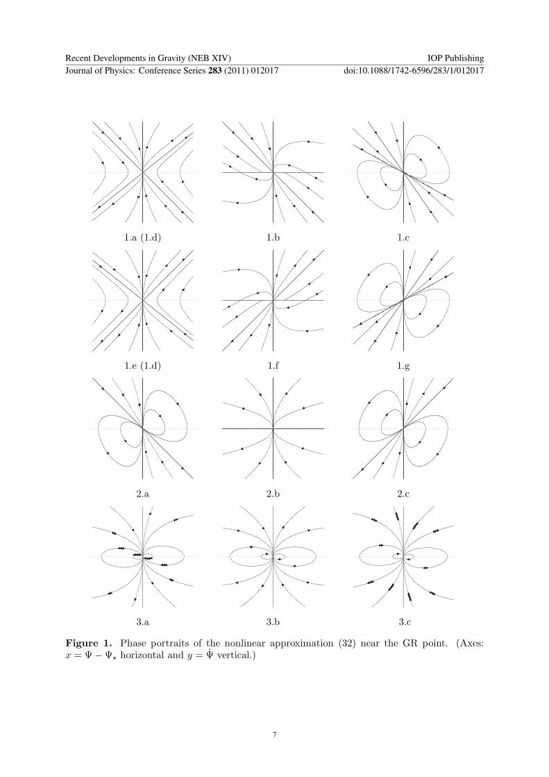