Scalable K-Means++

Bahman Bahmani∗†Stanford University

Stanford, CAbahman@stanford.edu

Benjamin Moseley∗‡University of Illinois

Urbana, ILbmosele2@illinois.edu

Andrea Vattani∗§University of California

San Diego, CA

avattani@cs.ucsd.eduRavi Kumar

Yahoo! ResearchSunnyvale, CA

ravikumar@yahoo-inc.com

Sergei VassilvitskiiYahoo! Research

New York, NYsergei@yahoo-inc.com

ABSTRACTOver half a century old and showing no signs of aging,k-means remains one of the most popular data process-ing algorithms. As is well-known, a proper initializationof k-means is crucial for obtaining a good final solution.The recently proposed k-means++ initialization algorithmachieves this, obtaining an initial set of centers that is prov-ably close to the optimum solution. A major downside of thek-means++ is its inherent sequential nature, which limits itsapplicability to massive data: one must make k passes overthe data to find a good initial set of centers. In this work weshow how to drastically reduce the number of passes neededto obtain, in parallel, a good initialization. This is unlikeprevailing efforts on parallelizing k-means that have mostlyfocused on the post-initialization phases of k-means. Weprove that our proposed initialization algorithm k-means||obtains a nearly optimal solution after a logarithmic num-ber of passes, and then show that in practice a constantnumber of passes suffices. Experimental evaluation on real-world large-scale data demonstrates that k-means|| outper-forms k-means++ in both sequential and parallel settings.

1. INTRODUCTIONClustering is a central problem in data management and

has a rich and illustrious history with literally hundreds ofdifferent algorithms published on the subject. Even so, a

∗Part of this work was done while the author was visitingYahoo! Research.†Research supported in part by William R. Hewlett Stan-ford Graduate Fellowship, and NSF awards 0915040 and IIS-0904325.‡Partially supported by NSF grant CCF-1016684.§Partially supported by NSF grant #0905645.

single method — k-means — remains the most popular clus-tering method; in fact, it was identified as one of the top 10algorithms in data mining [34]. The advantage of k-meansis its simplicity: starting with a set of randomly chosen ini-tial centers, one repeatedly assigns each input point to itsnearest center, and then recomputes the centers given thepoint assignment. This local search, called Lloyd’s itera-tion, continues until the solution does not change betweentwo consecutive rounds.

The k-means algorithm has maintained its popularity evenas datasets have grown in size. Scaling k-means to massivedata is relatively easy due to its simple iterative nature.Given a set of cluster centers, each point can independentlydecide which center is closest to it and, given an assignmentof points to clusters, computing the optimum center can bedone by simply averaging the points. Indeed parallel imple-mentations of k-means are readily available (see, for exam-ple, cwiki.apache.org/MAHOUT/k-means-clustering.html).

From a theoretical standpoint, k-means is not a good clus-tering algorithm in terms of efficiency or quality: the run-ning time can be exponential in the worst case [32, 4] andeven though the final solution is locally optimal, it can bevery far away from the global optimum (even under repeatedrandom initializations). Nevertheless, in practice the speedand simplicity of k-means cannot be beat. Therefore, recentwork has focused on improving the initialization procedure:deciding on a better way to initialize the clustering dramati-cally changes the performance of the Lloyd’s iteration, bothin terms of quality and convergence properties.

A important step in this direction was taken by Ostro-vsky et al. [30] and Arthur and Vassilvitskii [5], who showeda simple procedure that both leads to good theoretical guar-antees for the quality of the solution, and, by virtue of a goodstarting point, improves upon the running time of Lloyd’siteration in practice. Dubbed k-means++, the algorithm se-lects only the first center uniformly at random from the data.Each subsequent center is selected with a probability pro-portional to its contribution to the overall error given theprevious selections (we make this statement precise in Sec-tion 3). Intuitively, the initialization algorithm exploits thefact that a good clustering is relatively spread out, thuswhen selecting a new cluster center, preference should begiven to those further away from the previously selected cen-ters. Formally, one can show that k-means++ initialization

Permission to make digital or hard copies of all or part of this work forpersonal or classroom use is granted without fee provided that copies arenot made or distributed for profit or commercial advantage and that copiesbear this notice and the full citation on the first page. To copy otherwise, torepublish, to post on servers or to redistribute to lists, requires prior specificpermission and/or a fee. Articles from this volume were invited to presenttheir results at The 38th International Conference on Very Large Data Bases,August 27th - 31st 2012, Istanbul, Turkey.Proceedings of the VLDB Endowment, Vol. 5, No. 7Copyright 2012 VLDB Endowment 2150-8097/12/03... $ 10.00.

622

leads to an O(log k) approximation of the optimum [5], ora constant approximation if the data is known to be well-clusterable [30]. The experimental evaluation of k-means++initialization and the variants that followed [1, 2, 15] demon-strated that correctly initializing Lloyd’s iteration is crucialif one were to obtain a good solution not only in theory, butalso in practice. On a variety of datasets k-means++ initial-ization obtained order of magnitude improvements over therandom initialization.

The downside of the k-means++ initialization is its inher-ently sequential nature. Although its total running time ofO(nkd), when looking for a k-clustering of n points in Rd,is the same as that of a single Lloyd’s iteration, it is not ap-parently parallelizable. The probability with which a pointis chosen to be the ith center depends critically on the real-ization of the previous i−1 centers (it is the previous choicesthat determine which points are away in the current solu-tion). A naive implementation of k-means++ initializationwill make k passes over the data in order to produce theinitial centers.

This fact is exacerbated in the massive data scenario.First, as datasets grow, so does the number of classes intowhich one wishes to partition the data. For example, clus-tering millions of points into k = 100 or k = 1000 is typical,but a k-means++ initialization would be very slow in thesecases. This slowdown is even more detrimental when therest of the algorithm (i.e., Lloyd’s iterations) can be imple-mented in a parallel environment like MapReduce [13]. Formany applications it is desirable to have an initialization al-gorithm with similar guarantees to k-means++ and that canbe efficiently parallelized.

1.1 Our contributionsIn this work we obtain a parallel version of the k-means++

initialization algorithm and empirically demonstrate its prac-tical effectiveness. The main idea is that instead of samplinga single point in each pass of the k-means++ algorithm, wesample O(k) points in each round and repeat the process forapproximately O(logn) rounds. At the end of the algorithmwe are left with O(k logn) points that form a solution that iswithin a constant factor away from the optimum. We thenrecluster these O(k logn) points into k initial centers for theLloyd’s iteration. This initialization algorithm, which wecall k-means||, is quite simple and lends itself to easy paral-lel implementations. However, the analysis of the algorithmturns out to be highly non-trivial, requiring new insights,and is quite different from the analysis of k-means++.

We then evaluate the performance of this algorithm onreal-world datasets. Our key observations in the experi-ments are:

• O(logn) iterations is not necessary and after as little asfive rounds, the solution of k-means|| is consistently asgood or better than that found by any other method.

• The parallel implementation of k-means|| is much fasterthan existing parallel algorithms for k-means.

• The number of iterations until Lloyd’s algorithm con-verges is smallest when using k-means|| as the seed.

2. RELATED WORKClustering problems have been frequent and important

objects of study for the past many years by data manage-ment and data mining researchers.1 A thorough review ofthe clustering literature, even restricted to the work in thedatabase area, is far beyond the scope of this paper; thereaders are referred to the plethora of surveys available [8,10, 25, 21, 19]. Below, we only discuss the highlights directlyrelevant to our work.

Recall that we are concerned with k-partition clustering:given a set of n points in Euclidean space and an integerk, find a partition of these points into k subsets, each witha representative, also known as a center. There are threecommon formulations of k-partition clustering depending onthe particular objective used: k-center, where the objectiveis to minimize the maximum distance between a point andits nearest cluster center, k-median, where the objective isto minimize the sum of these distances, and k-means, wherethe objective is to minimize the sum of squares of thesedistances. All three of these problems are NP-hard, but aconstant factor approximation is known for them.

The k-means algorithms have been extensively studiedfrom database and data management points of view; we dis-cuss some of them. Ordonez and Omiecinski [29] studiedefficient disk-based implementation of k-means, taking intoaccount the requirements of a relational DBMS. Ordonez[28] studied SQL implementations of the k-means to betterintegrate it with a relational DBMS. The scalability issuesin k-means are addressed by Farnstrom et al. [16], whoused compression-based techniques of Bradley et al. [9] toobtain a single-pass algorithm. Their emphasis is to initial-ize k-means in the usual manner, but instead improve theperformance of the Lloyd’s iteration.

The k-means algorithm has also been considered in a par-allel and other settings; the literature is extensive on thistopic. Dhillon and Modha [14] considered k-means in themessage-passing model, focusing on the speed up and scal-ability issues in this model. Several papers have studiedk-means with outliers; see, for example, [22] and the refer-ences in [18]. Das et al. [12] showed how to implement EM(a generalization of k-means) in MapReduce; see also [36]who used similar tricks to speed up k-means. Sculley [31]presented modifications to k-means for batch optimizationsand to take data sparsity into account. None of these papersfocuses on doing a non-trivial initialization. More recently,Ene et al. [15] considered the k-median problem in MapRe-duce and gave a constant-round algorithm that achieves aconstant approximation.

The k-means algorithms have also been studied from the-oretical and algorithmic points of view. Kanungo et al. [23]proposed a local search algorithm for k-means with a run-ning time of O(n3ε−d) and an approximation factor of 9+ ε.Although the running time is only cubic in the worst case,even in practice the algorithm exhibits slow convergence tothe optimal solution. Kumar, Sabharwal, and Sen [26] ob-tained a (1 + ε)-approximation algorithm with a runningtime linear in n and d but exponential in k and 1

ε. Os-

trovsky et al. [30] presented a simple algorithm for findingan initial set of clusters for Lloyd’s iteration and showedthat under some data separability assumptions, the algo-

1A paper on database clustering [35] won the 2006 SIGMODTest of Time Award.

623

rithms achieve an O(1)-approximation to the optimum. Asimilar method, k-means++, was independently developedby Arthur and Vassilvitskii [5] who showed that it achievesan O(log k)-approximation but without any assumptions onthe data.

Since then, the k-means++ algorithm has been extended towork better on large datasets in the streaming setting. Ailonet al. [2] introduced a streaming algorithm inspired by thek-means++ algorithm. Their algorithm makes a single passover the data while selecting O(k log k) points and achievesa constant-factor approximation in expectation. Their al-gorithm builds on an influential paper of Guha et al. [17]who gave a streaming algorithm for the k-median problemthat is easily adaptable to the k-means setting. Ackermannet al. [1] introduced another streaming algorithm based onk-means++ and show that it performs well while making asingle pass over the input.

We will use MapReduce to demonstrate the effectivenessof our parallel algorithm, but note that the algorithm can beimplemented in a variety of parallel computational models.We require only primitive operations that are readily avail-able in any parallel setting. Since the pioneering work byDean and Ghemawat [13], MapReduce and its open sourceversion, Hadoop [33], has become a de facto standard forlarge data analysis, and a variety of algorithms have beendesigned for it [7, 6]. To aid in the formal analysis of MapRe-duce algorithms, Karloff et al. [24] introduced a model ofcomputation for MapReduce, which has since been used toreason about algorithms for set cover [11], graph problems[27], and other clustering formulations [15].

3. THE ALGORITHMIn this section we present our parallel algorithm for ini-

tializing Lloyd’s iteration. First, we set up some notationthat will be used throughout the paper. Next, we presentthe background on k-means clustering and the k-means++initialization algorithm (Section 3.1). Then, we present ourparallel initialization algorithm, which we call k-means|| (Sec-tion 3.3). We present an intuition why k-means|| initializa-tion can provide approximation guarantees (Section 3.4); theformal analysis is deferred to Section 6. Finally, we discussa MapReduce realization of our algorithm (Section 3.5).

3.1 Notation and backgroundLetX = x1, . . . , xn be a set of points in the d-dimensional

Euclidean space and let k be a positive integer specifyingthe number of clusters. Let ||xi − xj || denote the Euclideandistance between xi and xj . For a point x and a subsetY ⊆ X of points, the distance is defined as d(x, Y ) =miny∈Y ||x − y||. For a subset Y ⊆ X of points, let itscentroid be given by

centroid(Y ) =1

|Y |∑y∈Y

y.

Let C = c1, . . . , ck be a set of points and let Y ⊆ X.We define the cost of Y with respect to C as

φY (C) =∑y∈Y

d2(y, C) =∑y∈Y

mini=1,...,k

||y − ci||2.

The goal of k-means clustering is to choose a set C of k cen-ters to minimize φX(C); when it is obvious from the context,

we simply denote this as φ. Let φ∗ be the cost of the opti-mal k-means clustering; finding φ∗ is NP-hard [3]. We calla set C of centers to be an α-approximation to k-means ifφX(C) ≤ αφ∗. Note that the centers automatically define aclustering of X as follows: the ith cluster is the set of allpoints in X that are closer to ci than any other cj , j 6= i.

We now describe the popular method for finding a locallyoptimum solution to the k-means problem. It starts with arandom set of k centers. In each iteration, a clustering of Xis derived from the current set of centers. The centroids ofthese derived clusters then become the centers for the nextiteration. The iteration is then repeated until a stable setof centers is obtained. The iterative portion of the abovemethod is called Lloyd’s iteration.

Arthur and Vassilvitskii [5] modified the initialization stepin a careful manner and obtained a randomized initializa-tion algorithm called k-means++. The main idea in theiralgorithm is to choose the centers one by one in a controlledfashion, where the current set of chosen centers will stochas-tically bias the choice of the next center (Algorithm 1). Theadvantage of k-means++ is that even the initialization stepitself obtains an (8 log k)-approximation to φ∗ in expectation(running Lloyd’s iteration on top of this will only improvethe solution, but no guarantees can be made). The cen-tral drawback of k-means++ initialization from a scalabilitypoint of view is its inherent sequential nature: the choice ofthe next center depends on the current set of centers.

Algorithm 1 k-means++(k) initialization.

1: C ← sample a point uniformly at random from X2: while |C| < k do

3: Sample x ∈ X with probability d2(x,C)φX (C)

4: C ← C ∪ x5: end while

3.2 Intuition behind our algorithmWe describe the high-level intuition behind our algorithm.

It is easiest to think of random initialization and k-means++initialization as occurring at two ends of a spectrum. Theformer selects k centers in a single iteration according to aspecific distribution, which is the uniform distribution. Thelatter has k iterations and selects one point in each iterationaccording to a non-uniform distribution (that is constantlyupdated after each new center is selected). The provablegains of k-means++ over random initialization is preciselyin the constantly updated non-uniform selection. Ideally,we would like to achieve the best of both worlds: an algo-rithm that works in a small number of iterations, selectsmore than one point in each iteration but in a non-uniformmanner, and has provable approximation guarantees. Ouralgorithm follows this intuition and finds the sweet spot (orthe best trade-off point) on the spectrum by carefully defin-ing the number of iterations and the non-uniform distribu-tion itself. While the above idea seems conceptually simple,making it work with provable guarantees (as k-means++)throws up a lot of challenges, some of which are also clearlyreflected in the analysis of our algorithm. We now describeour algorithm.

624

3.3 Our initialization algorithm: k-means||In this section we present k-means||, our parallel version

for initializing the centers. While our algorithm is largelyinspired by k-means++, it uses an oversampling factor ` =Ω(k), which is unlike k-means++; intuitively, ` should bethought of as Θ(k). Our algorithm picks an initial center(say, uniformly at random) and computes ψ, the initial costof the clustering after this selection. It then proceeds in logψiterations, where in each iteration, given the current set C ofcenters, it samples each x with probability `d2(x, C)/φX(C).The sampled points are then added to C, the quantity φX(C)updated, and the iteration continued. As we will see later,

Algorithm 2 k-means||(k, `) initialization.

1: C ← sample a point uniformly at random from X2: ψ ← φX(C)3: for O(logψ) times do4: C′ ← sample each point x ∈ X independently with

probability px = `·d2(x,C)φX (C)

5: C ← C ∪ C′6: end for7: For x ∈ C, set wx to be the number of points in X closer

to x than any other point in C8: Recluster the weighted points in C into k clusters

the expected number of points chosen in each iteration is `and at the end, the expected number of points in C is ` logψ,which is typically more than k. To reduce the number ofcenters, Step 7 assigns weights to the points in C and Step8 reclusters these weighted points to obtain k centers. Thedetails are presented in Algorithm 2.

Notice that the size of C is significantly smaller than theinput size; the reclustering can therefore be done quickly.For instance, in MapReduce, since the number of centersis small they can all be assigned to a single machine andany provable approximation algorithm (such as k-means++)can be used to cluster the points to obtain k centers. AMapReduce implementation of Algorithm 2 is discussed inSection 3.5.

While our algorithm is very simple and lends itself to anatural parallel implementation (in logψ rounds2), the chal-lenging part is to show that it has provable guarantees. Notethat ψ ≤ n2∆2, where ∆ is the maximum distance among apair of points in X.

We now state our formal guarantee about this algorithm.

Theorem 1. If an α-approximation algorithm is used inStep 8, then Algorithm k-means|| obtains a solution that isan O(α)-approximation to k-means.

Thus, if k-means++ initialization is used in Step 8, thenk-means|| is an O(log k)-approximation. In Section 3.4 wegive an intuitive explanation why the algorithm works; wedefer the full proof to Section 6.

3.4 A glimpse of the analysisIn this section, we present the intuition behind the proof

of Theorem 1. Consider a cluster A present in the optimumk-means solution, denote |A| = T , and sort the points in Ain an increasing order of their distance to centroid(A): let

2In practice, our experimental results in Section 5 show thatonly a few rounds are enough to reach a good solution.

the ordering be a1, . . . , aT . Let qt be the probability thatat is the first point in the ordering chosen by k-means|| andqT+1 be the probability that no point is sampled from clusterA. Letting pt denote the probability of selecting at, we have,by definition of the algorithm, pt = `d2(at, C)/φX(C). Also,since k-means|| picks each point independently, for any 1 ≤t ≤ T , we have qt = pt

∏t−1j=1(1−pj), and qT+1 = 1−

∑Tt=1 qt.

If at is the first point in A (w.r.t. the ordering) sampledas a new center, we can either assign all the points in A toat, or just stick with the current clustering of A. Hence,letting

st = min

φA,

∑a∈A

||a− at||2,

we have

E[φA(C ∪ C′)] ≤T∑t=1

qtst + qT+1φA(C),

Now, we do a mean-field analysis, in which we assume allpt’s (1 ≤ t ≤ T ) to be equal to some value p. Geometricallyspeaking, this corresponds to the case where all the pointsin A are very far from the current clustering (and are alsorather tightly clustered, so that all d(at, C)’s (1 ≤ t ≤ T )are equal). In this case, we have qt = p(1 − p)t−1, andhence qt1≤t≤T is a monotone decreasing sequence. By theordering on at’s, letting

s′t =∑a∈A

||a− at||2,

we have that s′t1≤t≤T is an increasing sequence. Therefore

T∑t=1

qtst ≤T∑t=1

qts′t ≤

1

T

(T∑t=1

qt ·T∑t=1

s′t

),

where the last inequality, an instance of Chebyshev’s sum in-equality [20], is using the inverse monotonicity of sequences

qt1≤t≤T and s′t1≤t≤T . It is easy to see that 1T

∑Tt=1 s

′t =

2φ∗A. Therefore,

E[φA(C ∪ C′)] ≤ (1− qT+1)2φ∗A + qT+1φA(C).

This shows that in each iteration of k-means||, for eachoptimal cluster A, we remove a fraction of φA and replaceit with a constant factor times φ∗A. Thus, Steps 1–6 ofk-means|| obtain a constant factor approximation to k-meansafter O(logψ) rounds and return O(` logψ) centers. The al-gorithm obtains a solution of size k by clustering the chosencenters using a known algorithm. Section 6 contains the for-mal arguments that work for the general case when pt’s arenot necessarily the same.

3.5 A parallel implementationIn this section we discuss a parallel implementation of

k-means|| in the MapReduce model of computation. Weassume familiarity with the MapReduce model and refer thereader to [13] for further details. As we mentioned earlier,Lloyd’s iterations can be easily parallelized in MapReduceand hence, we only focus on Steps 1–7 in Algorithm 2. Step4 is very simple in MapReduce: each mapper can sampleindependently and Step 7 is equally simple given a set C ofcenters. Given a (small) set C of centers, computing φX(C)is also easy: each mapper working on an input partitionX ′ ⊆ X can compute φX′(C) and the reducer can simply

625

add these values from all mappers to obtain φX(C). Thistakes care of Step 2 and the update to φX(C) needed for theiteration in Steps 3–6.

Note that we have tacitly assumed that the set C of cen-ters is small enough to be held in memory or be distributedamong all the mappers. While this suffices for nearly allpractical settings, it is possible to implement the above stepsin MapReduce even without this assumption. Each map-per holding X ′ ⊆ X and C′ ⊆ C can output the tuple〈x; arg minc∈C′ d(x, c)〉, where x ∈ X ′ is the key. From this,the reducer can easily compute d(x, C) and hence φX(C). Re-ducing the amount of intermediate output by the mappersin this case is an interesting research direction.

4. EXPERIMENTAL SETUPIn this section we present the experimental setup for eval-

uating k-means||. The sequential version of algorithms wereevaluated on a single workstation with quad-core 2.5GHzprocessors and 16Gb of memory. The parallel algorithmswere run using a Hadoop cluster of 1968 nodes, each withtwo quad-core 2.5GHz processors and 16GB of memory.

We describe the datasets and baseline algorithms that willbe used for comparison.

4.1 DatasetsWe use three datasets to evaluate the performance of

k-means||. The first dataset, GaussMixture, is synthetic;a similar version was used in [5]. To generate the dataset,we sampled k centers from a 15-dimensional spherical Gaus-sian distribution with mean at the origin and variance R ∈1, 10, 100. We then added points from Gaussian distribu-tions of unit variance around each center. Given the k cen-ters, this is a mixture of k spherical Gaussians with equalweights. Note that the Gaussians are separated in termsof probability mass — even if only marginally for the caseR = 1 — and therefore the value of the optimal k-clusteringcan be well approximated using the centers of these Gaus-sians. The number of sampled points from this mixture ofGaussians is n = 10, 000.

The other two datasets considered are from real-world set-tings and are publicly available from the UC Irvine MachineLearning repository (archive.ics.uci.edu/ml/datasets.html). The Spam dataset consists of 4601 points in 58 di-mensions and represents features available to an e-mail spamdetection system. The KDDCup1999 dataset consists of4.8M points in 42 dimensions and was used for the 1999KDD Cup. We also used a 10% sample of this dataset toillustrate the effect of different parameter settings.

For GaussMixture and Spam, given the moderate num-ber of points in those datasets, we use k ∈ 20, 50, 100.For KDDCup1999, we experiment with finer clusterings,i.e., we use k ∈ 500, 1000. The datasets GaussMixtureand Spam are studied with the sequential implementation ofk-means||, whereas we use the parallel implementation (inthe Hadoop framework) for KDDCup1999.

4.2 BaselinesFor the rest of the paper, we assume that each initializa-

tion method is implicitly followed by Lloyd’s iterations. Wecompare the performance of k-means|| initialization againstthe following baselines:

• k-means++ initialization, as in Algorithm 1;

• Random, which selects k points uniformly at randomfrom the dataset; and

• Partition, which is a recent streaming algorithm fork-means clustering [2], described in Section 4.2.1.

Of these, k-means++ can be viewed as the true baseline,since k-means|| is a natural parallelization of it. However,k-means++ can be only run on datasets of moderate sizeand only for modest values of k. For large-scale datasets,it becomes infeasible and parallelization becomes necessary.Since Random is commonly used and is easily parallelized, wechose it as one of our baselines. Finally, Partition is a re-cent one-pass streaming algorithm with performance guar-antees, and is also parallelizable; hence, we included it aswell in our baseline and describe it in Section 4.2.1. We nowdescribe the parameter settings for these algorithms.

For Random, the parallel MapReduce/Hadoop implemen-tation is standard3. In the sequential setting we ran Random

until convergence, while in the parallel version, we boundedthe number of iterations to 20. In general, we observedthat the improvement in the cost of the clustering becomesmarginal after only a few iterations. Furthermore, takingthe best of Random repeated multiple times with differentrandom initial points also obtained only marginal improve-ments in the clustering cost.

We use k-means++ for reclustering in Step 8 of k-means||.We tested k-means|| with ` ∈ 0.1k, 0.5k, k, 2k, 10k, withr = 15 rounds for the case ` = 0.1k, and r = 5 roundsotherwise (running k-means|| for five rounds when ` = 0.1kleads it to select fewer than k centers with high probabil-ity). Since the expected number of intermediate points con-sidered by k-means|| is r`, these settings of the parametersyield a very small intermediate set (of size between 1.5k and40k). Nonetheless, the quality of the solutions returned byk-means|| is comparable and often better than Partition,which makes use of a much larger set and hence is muchslower.

4.2.1 Setting parameters for Partition

The Partition algorithm [2] takes as input a parametermand works as follows: it divides the input into m equal-sizedgroups. In each group, it runs a variant of k-means++ thatselects 3 log k points in each iteration (traditional k-means++selects only a single point). At the end of this, similar toour reclustering step, it runs (vanilla) k-means++ on theweighted set of these 3m log k clusters to reduce the numberof centers to k.

Choosing m =√n/k minimizes the amount of mem-

ory used by the streaming algorithm. A neat feature ofPartition is that it can be implemented in parallel: in thefirst round, groups are assigned to m different machines thatcan be run in parallel to obtain the intermediate set and inthe second round, k-means++ is run on this set sequentially.In the parallel implementation, the setting m =

√n/k not

only optimizes the memory used by each machine but alsooptimizes the total running time of the algorithm (ignor-ing setup costs), as the size of the instance per machine inthe two rounds is equated. (The instance size per machine

is O(n/m) = O(√nk) which yields a running time in each

3E.g., cwiki.apache.org/MAHOUT/k-means-clustering.html.

626

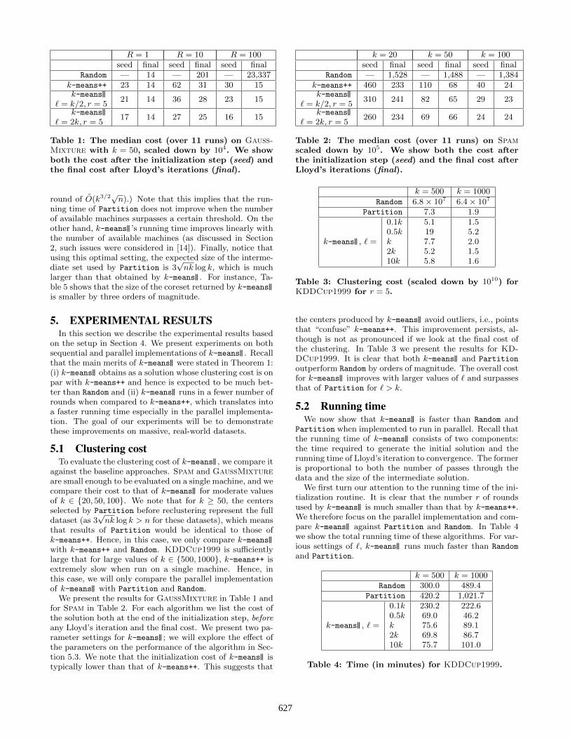
R = 1 R = 10 R = 100seed final seed final seed final

Random — 14 — 201 — 23,337k-means++ 23 14 62 31 30 15k-means||

` = k/2, r = 521 14 36 28 23 15

k-means||` = 2k, r = 5

17 14 27 25 16 15

Table 1: The median cost (over 11 runs) on Gauss-Mixture with k = 50, scaled down by 104. We showboth the cost after the initialization step (seed) andthe final cost after Lloyd’s iterations (final).

round of O(k3/2√n).) Note that this implies that the run-

ning time of Partition does not improve when the numberof available machines surpasses a certain threshold. On theother hand, k-means||’s running time improves linearly withthe number of available machines (as discussed in Section2, such issues were considered in [14]). Finally, notice thatusing this optimal setting, the expected size of the interme-diate set used by Partition is 3

√nk log k, which is much

larger than that obtained by k-means||. For instance, Ta-ble 5 shows that the size of the coreset returned by k-means||is smaller by three orders of magnitude.

5. EXPERIMENTAL RESULTSIn this section we describe the experimental results based

on the setup in Section 4. We present experiments on bothsequential and parallel implementations of k-means||. Recallthat the main merits of k-means|| were stated in Theorem 1:(i) k-means|| obtains as a solution whose clustering cost is onpar with k-means++ and hence is expected to be much bet-ter than Random and (ii) k-means|| runs in a fewer number ofrounds when compared to k-means++, which translates intoa faster running time especially in the parallel implementa-tion. The goal of our experiments will be to demonstratethese improvements on massive, real-world datasets.

5.1 Clustering costTo evaluate the clustering cost of k-means||, we compare it

against the baseline approaches. Spam and GaussMixtureare small enough to be evaluated on a single machine, and wecompare their cost to that of k-means|| for moderate valuesof k ∈ 20, 50, 100. We note that for k ≥ 50, the centersselected by Partition before reclustering represent the fulldataset (as 3

√nk log k > n for these datasets), which means

that results of Partition would be identical to those ofk-means++. Hence, in this case, we only compare k-means||with k-means++ and Random. KDDCup1999 is sufficientlylarge that for large values of k ∈ 500, 1000, k-means++ isextremely slow when run on a single machine. Hence, inthis case, we will only compare the parallel implementationof k-means|| with Partition and Random.

We present the results for GaussMixture in Table 1 andfor Spam in Table 2. For each algorithm we list the cost ofthe solution both at the end of the initialization step, beforeany Lloyd’s iteration and the final cost. We present two pa-rameter settings for k-means||; we will explore the effect ofthe parameters on the performance of the algorithm in Sec-tion 5.3. We note that the initialization cost of k-means|| istypically lower than that of k-means++. This suggests that

k = 20 k = 50 k = 100seed final seed final seed final

Random — 1,528 — 1,488 — 1,384k-means++ 460 233 110 68 40 24k-means||

` = k/2, r = 5310 241 82 65 29 23

k-means||` = 2k, r = 5

260 234 69 66 24 24

Table 2: The median cost (over 11 runs) on Spamscaled down by 105. We show both the cost afterthe initialization step (seed) and the final cost afterLloyd’s iterations (final).

k = 500 k = 1000Random 6.8× 107 6.4× 107

Partition 7.3 1.90.1k 5.1 1.50.5k 19 5.2

k-means||, ` = k 7.7 2.02k 5.2 1.510k 5.8 1.6

Table 3: Clustering cost (scaled down by 1010) forKDDCup1999 for r = 5.

the centers produced by k-means|| avoid outliers, i.e., pointsthat “confuse” k-means++. This improvement persists, al-though is not as pronounced if we look at the final cost ofthe clustering. In Table 3 we present the results for KD-DCup1999. It is clear that both k-means|| and Partition

outperform Random by orders of magnitude. The overall costfor k-means|| improves with larger values of ` and surpassesthat of Partition for ` > k.

5.2 Running timeWe now show that k-means|| is faster than Random and

Partition when implemented to run in parallel. Recall thatthe running time of k-means|| consists of two components:the time required to generate the initial solution and therunning time of Lloyd’s iteration to convergence. The formeris proportional to both the number of passes through thedata and the size of the intermediate solution.

We first turn our attention to the running time of the ini-tialization routine. It is clear that the number r of roundsused by k-means|| is much smaller than that by k-means++.We therefore focus on the parallel implementation and com-pare k-means|| against Partition and Random. In Table 4we show the total running time of these algorithms. For var-ious settings of `, k-means|| runs much faster than Random

and Partition.

k = 500 k = 1000Random 300.0 489.4

Partition 420.2 1,021.70.1k 230.2 222.60.5k 69.0 46.2

k-means||, ` = k 75.6 89.12k 69.8 86.710k 75.7 101.0

Table 4: Time (in minutes) for KDDCup1999.

627

While one can expect k-means|| to be faster than Random,we investigate the reason why k-means|| runs faster thanPartition. Recall that both k-means|| and Partition firstselect a large number of centers and then recluster the cen-ters to find the k initial points. In Table 5 we show the totalnumber of intermediate centers chosen both by k-means||and Partition before reclustering on KDDCup1999. Weobserve that k-means|| is more judicious in selecting cen-ters, and typically selects only 10–40% as many centers asPartition, which directly translates into a faster runningtime, without sacrificing the quality of the solution. Select-ing fewer points in the intermediate state directly translatesto the observed speedup.

k = 500 k = 1000Partition 9.5× 105 1.47× 106

0.1k 602 1,2400.5k 591 1,124

k-means||, ` = k 1,074 2,2342k 2,321 3,60410k 9,116 7,588

Table 5: Number of centers for KDDCup1999 beforethe reclustering.

We next show an unexpected benefit of k-means||: initialsolution found by k-means|| leads to a faster convergence ofthe Lloyd’s iteration. In Table 6 we show the number ofiterations to convergence of Lloyd’s iterations for differentinitializations. We observe that k-means|| typically requiresfewer iterations than k-means++ to converge to a local op-timum, and both converge significantly faster than Random.

k = 20 k = 50 k = 100Random 176.4 166.8 60.4

k-means++ 38.3 42.2 36.6k-means||` = 0.5k, r = 5

36.9 30.8 30.2

k-means||` = 2k, r = 5

23.3 28.1 29.7

Table 6: Number of Lloyd’s iterations till conver-gence (averaged over 10 runs) for Spam.

5.3 Trading-off quality with running timeBy changing the number r of rounds, k-means|| interpo-

lates between a purely random initialization of k-means andthe biased sequential initialization of k-means++. Whenr = 0 all of the points are sampled uniformly at random,simulating the Random initialization, and when r = k, thealgorithm updates the probability distribution at every step,simulating k-means++. In this section we explore this trade-off. There is an additional technicality that we must becognizant of: whereas k-means++ draws a single center fromthe joint distribution induced by D2 weighting, k-means|| se-lects each point independently with probability proportionalto D2, selecting ` points in expectation.

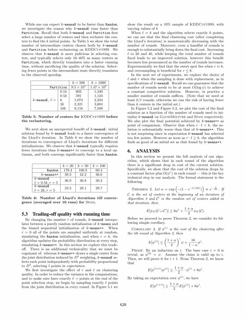
We first investigate the effect of r and ` on clusteringquality. In order to reduce the variance in the computations,and to make sure have exactly ` · r points at the end of thepoint selection step, we begin by sampling exactly ` pointsfrom the joint distribution in every round. In Figure 5.1 we

show the result on a 10% sample of KDDCup1999, withvarying values of k

When ` = k and the algorithm selects exactly k points,we can see that the final clustering cost (after completingthe Lloyd’s iteration) is monotonically decreasing with thenumber of rounds. Moreover, even a handful of rounds isenough to substantially bring down the final cost. Increasing` to 2k and 4k, while keeping the total number of roundsfixed leads to an improved solution, however this benefitbecomes less pronounced as the number of rounds increases.Experimentally we find that the sweet spot lies when r ≈ 8,and oversampling is beneficial for r ≤ 8.

In the next set of experiments, we explore the choice of` and r when the sampling is done with replacement, as inspecifications of k-means||. Recall we can guarantee that thenumber of rounds needs to be at most O(logψ) to achievea constant competitive solution. However, in practice asmaller number of rounds suffices. (Note that we need atleast k/` rounds, otherwise we run the risk of having fewerthan k centers in the initial set.)

In Figure 5.2 and Figure 5.3, we plot the cost of the finalsolution as a function of the number of rounds used to ini-tialize k-means|| on GaussMixture and Spam respectively.We also plot the final potential achieved by k-means++ aspoint of comparison. Observe that when r · ` < k, the so-lution is substantially worse than that of k-means++. Thisis not surprising since in expectation k-means|| has selectedtoo few points. However as soon as r · ` ≥ k, the algorithmfinds as good of an initial set as that found by k-means++.

6. ANALYSISIn this section we present the full analysis of our algo-

rithm, which shows that in each round of the algorithmthere is a significant drop in cost of the current solution.Specifically, we show that the cost of the solution drops bya constant factor plus O(φ∗) in each round — this is the keytechnical step in our analysis. The formal statement is thefollowing.

Theorem 2. Let α = exp(−(1− e−`/(2k))

)≈ e−

`2k . If

C is the set of centers at the beginning of an iteration ofAlgorithm 2 and C′ is the random set of centers added inthat iteration, then

E[φX(C ∪ C′)] ≤ 8φ∗ +1 + α

2φX(C).

Before we proceed to prove Theorem 2, we consider its fol-lowing simple corollary.

Corollary 3. If φ(i) is the cost of the clustering afterthe ith round of Algorithm 2, then

E[φ(i)] ≤(

1 + α

2

)iψ +

16

1− αφ∗.

Proof. By an induction on i. The base case i = 0 istrivial, as φ(0) = ψ. Assume the claim is valid up to i.Then, we will prove it for i+ 1. From Theorem 2, we knowthat

E[φ(i+1)|φ(i)] ≤ 1 + α

2· φ(i) + 8φ∗.

By taking an expectation over φ(i), we have

E[φ(i+1)] ≤ 1 + α

2E[φ(i)] + 8φ∗.

628

1e+12

1e+13

1e+14

1e+15

1e+16

1 10

cost

log # Rounds

KDD Dataset, k=17

l/k=1l/k=2l/k=4

1e+11

1e+12

1e+13

1e+14

1e+15

1e+16

1 10

cost

log # Rounds

KDD Dataset, k=33

l/k=1l/k=2l/k=4

1e+11

1e+12

1e+13

1e+14

1e+15

1e+16

1 10

cost

log # Rounds

KDD Dataset, k=65

l/k=1l/k=2l/k=4

1e+10

1e+11

1e+12

1e+13

1e+14

1e+15

1e+16

1 10 100

cost

log # Rounds

KDD Dataset, k=129

l/k=1l/k=2l/k=4

Figure 5.1: The effect of different values of ` and the number of rounds r on the final cost of the algorithmfor a 10% sample of KDDCup1999. Each data point is the median of 11 runs of the algorithm.

By the induction hypothesis on E[φ(i)], we have

E[φ(i+1)] ≤(

1 + α

2

)i+1

ψ + 8

(1 + α

1− α + 1

)φ∗

=

(1 + α

2

)i+1

ψ +16

1− αφ∗.

Corollary 3 implies that after O(logψ) rounds, the cost ofthe clustering is O(φ∗); Theorem 1 is then an immediateconsequence. We now proceed to establish Theorem 2.

Consider any cluster A with centroid(A) in the optimalsolution. Denote |A| = T and let a1, . . . , aT be the pointsin A sorted increasingly with respect to their distance tocentroid(A). Let C′ denote the set of centers that are se-lected during a particular iteration. For 1 ≤ t ≤ T , welet

qt = Pr[at ∈ C′, aj /∈ C′, ∀ 1 ≤ j < t]

be the probability that the first t−1 points a1, . . . , at−1 arenot sampled during this iteration and at is sampled. Also,we denote by qT+1 the probability that no point is sampledfrom cluster A.

Furthermore, for the remainder of this section, let D(a) =d(a, C), where C is the set of centers in the current iteration.Letting pt denote the probability of selecting at, we have,

by definition of the algorithm, pt = `D2(at)φ

. Since k-means||picks each point independently, using the convention thatpT+1 = 1, we have for all 1 ≤ t ≤ T + 1,

qt = pt

t−1∏j=1

(1− pj).

The main idea behind the proof is to consider only thoseclusters in the optimal solution that have significant cost rel-ative to the total clustering cost. For each of these clusters,the idea is to first express both its clustering cost and theprobability that an early point is not selected as linear func-tions of the qt’s (Lemmas 4, 5), and then appeal to linearprogramming (LP) duality in order to bound the clusteringcost itself (Lemma 6 and Corollary 7). To formalize thisidea, we start by defining

st = min

φA,

∑a∈A

||a− at||2,

for all 1 ≤ t ≤ T , and sT+1 = φA. Then, letting φ′A =φA(C∪C′) be the clustering cost of cluster A after the currentround of the algorithm, we have the following.

629

0 5 10 15104

105

106

# Initialization Rounds

Cos

t

R=1

0 5 10 15104

105

106

107

108

# Initialization Rounds

Cos

t

R=10

0 5 10 15104

105

106

107

108

109

1010

# Initialization Rounds

Cos

t

R=100

0 5 10 15

105.2

105.4

105.6

105.8

# Initialization Rounds

Cos

t

R=1

0 5 10 15105

106

107

108

# Initialization Rounds

Cos

t

R=10

0 5 10 15105

106

107

108

109

1010

# Initialization Rounds

Cos

t

R=100

0 5 10 15

105.2

105.4

105.6

105.8

# Initialization Rounds

Cos

t

R=1

0 5 10 15105

106

107

108

# Initialization RoundsC

ost

R=10

0 5 10 15105

106

107

108

109

1010

# Initialization Rounds

Cos

t

R=100

KM++ & Lloydl/k=0.1l/k=0.5l/k=1l/k=2l/k=10

KM++l/k=0.1l/k=0.5l/k=1l/k=2l/k=10

Figure 5.2: The cost of k-means|| followed by Lloyd’s iterations as a function of the number of initializationrounds for GaussMixture.

Lemma 4. The expected cost of clustering an optimumcluster A after a round of Algorithm 2 is bounded as

E[φ′A] ≤T+1∑t=1

qtst. (6.1)

Proof. We can rewrite the expectation of the clusteringcost φ′A for cluster A after one round of the algorithm asfollows:

E[φ′A] =

T∑t=1

qtE[φ′A | at ∈ C′, aj /∈ C′, ∀ 1 ≤ j < t]. (6.2)

Observe that conditioned on the fact that at ∈ C′, we caneither assign all the points in A to center at, or just stickwith the former clustering of A, whichever has a smallercost. Hence

E[φ′A | at ∈ C′, aj /∈ C′,∀ 1 ≤ j < t] ≤ st.

and the result follows from (6.2).

In order to minimize the right hand side of (6.1), we wantto be sure that the sampling done by the algorithm placesa lot of weight on qt for small values of t. Intuitively thismeans that we are more likely to select a point close to theoptimal center of the cluster than one further away. Oursampling based on D2(·) implies a constraint on the prob-ability that an early point is not selected, which we detailbelow.

Lemma 5. Let η0 = 1, and, for any 1 ≤ t ≤ T , ηt =∏tj=1

(1− D2(aj)

φA(1− qT+1)

). Then, for any 0 ≤ t ≤ T ,

T+1∑r=t+1

qr ≤ ηt.

Proof. First note that qT+1 =∏Tt=1(1 − pt) ≥ 1 −∑T

t=1 pt. Therefore,

1− qT+1 ≤t∑t=1

pt = `φAφ.

Thus

pt =`D2(at)

φ≥ D2(at)

φA(1− qT+1).

To prove the lemma, by the definition of qr we have

T+1∑r=t+1

qr =

(t∏

j=1

(1− pj)

)·T+1∑r=t+1

r−1∏j=t+1

(1− pj)pr

≤t∏j=1

(1− pj)

≤t∏j=1

(1− D2(at)

φA(1− qT+1)

)= ηt.

Having proved this lemma, we now slightly change ourperspective and think of the values qt (1 ≤ t ≤ T + 1) asvariables that (by Lemma 5) satisfy a number of linear con-straints and also (by Lemma 4) a linear function of whichbounds E[φ′A]. This naturally leads to an LP on these vari-ables to get an upper bound on E[φ′A]; see Figure 6.1. Wewill then use the properties of the LP and its dual to provethe following lemma.

Lemma 6. The expected potential of an optimal cluster Aafter a sampling step in Algorithm 2 is bounded as

E[φ′A] ≤ (1− qT+1)

T∑t=1

D2(at)

φAst + ηTφA.

Proof. Since the points in A are sorted increasingly withrespect to their distances to the centroid, letting

s′t =∑a∈A

||a− at||2, (6.3)

for 1 ≤ t ≤ T , we have that s′1 ≤ · · · ≤ s′T . Hence, sincest = minφA, s′t, we also have s1 ≤ · · · ≤ sT ≤ sT+1.

Now consider the LP in Figure 6.1 and its dual. Since stis an increasing sequence, the optimal solution to the dualmust have αt = st+1 − st (letting s0 = 0). Then, we can

630

0 5 10 15104

105

106

107

108

109

1010

# Initialization Rounds

Cos

t

k=20

0 5 10 1510−5

100

105

1010

# Initialization Rounds

Cos

t

k=50

0 5 10 1510−5

100

105

1010

# Initialization Rounds

Cos

t

k=100

0 5 10 15107

108

109

1010

# Initialization Rounds

Cos

t

k=20

0 5 10 15106

107

108

109

1010

# Initialization Rounds

Cos

t

k=50

0 5 10 15106

107

108

109

1010

# Initialization Rounds

Cos

t

k=100

0 5 10 15107

108

109

1010

# Initialization Rounds

Cos

tk=20

0 5 10 15106

107

108

109

1010

# Initialization Rounds

Cos

t

k=50

0 5 10 15106

107

108

109

1010

# Initialization Rounds

Cos

t

k=100

l/k=0.1l/k=0.5l/k=1l/k=2l/k=10KM++

l/k=0.1l/k=0.5l/k=1l/k=2l/k=10KM++ & Lloyd

Figure 5.3: The cost of k-means|| followed by Lloyd’s iterations as a function of the number of initializationrounds for Spam.

maxq1,...,qT+1

T+1∑t=1

qtst

subject to

T+1∑r=t+1

qr ≤ ηt, (∀0 ≤ t ≤ T )

qt ≥ 0. (∀1 ≤ t ≤ T + 1)

minα0,...,αT

T∑t=0

ηtαt

subject to

t−1∑r=0

αr ≥ st, (∀1 ≤ t ≤ T + 1)

αt ≥ 0. (∀0 ≤ t ≤ T )

Figure 6.1: LP (left) and its dual (right).

bound the value of the dual (and hence the value of theprimal, which by Lemma 4 and Lemma 5 is an upper boundon E[φ′A]) as follows:

E[φ′A] ≤T∑t=0

ηtαt

=

T∑t=1

st(ηt−1 − ηt) + ηT sT+1

=

T∑t=1

stηt−1

(D2(at)

φA

)(1− qT+1) + ηT sT+1

≤ (1− qT+1)

T∑t=1

D2(at)

φAst + ηTφA,

where the last step follows since ηt ≤ 1.

This results in the following corollary:

Corollary 7.

E[φ′A] ≤ 8φ∗A(1− qT+1) + φAe−(1−qT+1).

Proof. By the triangle inequality, for all a, at we haveD(at) ≤ D(a) + ||a− at||. The power-mean inequality then

implies that D2(at) ≤ 2D2(a) + 2||a− at||2. Summing overall a ∈ A and dividing by φA, we have that

D2(at)

φA≤ 2

T+

2

T

s′tφA

,

where s′t is defined in (6.3). Hence,

T∑t=1

D2(at)

φAst ≤

T∑t=1

(2

T+

2

T

s′tφA

)st

=2

T

T∑t=1

st +2

T

T∑t=1

s′tstφA

≤ 2

T

T∑t=1

s′t +2

T

T∑t=1

s′t

= 8φ∗A,

where in the last inequality, we used st ≤ s′t for the firstsummation, and st ≤ φA for the second one.

631

Finally, noticing

ηT =

T∏j=1

(1− D2(aj)

φA(1− qT+1)

)

≤ exp

(−

T∑j=1

D2(aj)

φA(1− qT+1)

)= exp(−(1− qT+1)),

the proof follows from Lemma 6.

We are now ready to prove the main result.

Proof of Theorem 2. Let A1, . . . , Ak be the clusters inthe optimal solution Cφ∗ . We partition these clusters into“heavy” and “light” as follows:

CH =

A ∈ Cφ∗

∣∣ φAφ

>1

2k

, and

CL = Cφ∗ \ CH .Recall that

qT+1 =

T∏j=1

(1− pj) ≤ exp

(−∑j

pj

)= exp

(− `φA

φ

).

Then, by Corollary 7, for any heavy cluster A, we have

E[φ′A] ≤ 8φ∗A(1− qT+1) + φAe−(1−qT+1)

≤ 8φ∗A + exp(−(1− e−`/2k))φA

= 8φ∗A + αφA.

Summing up over all A ∈ CH , we get

E[φ′CH ] ≤ 8φ∗CH + αφCH .

Then, by noting that

φCL ≤φ

2k· |CL| ≤

φ

2kk =

φ

2,

and that E[φ′CL ] ≤ φCL , we have

E[φ′] ≤ 8φ∗CH + αφCH + φCL= 8φ∗CH + αφ+ (1− α)φCL≤ 8φ∗CH + (α+ (1− α)/2)φ

≤ 8φ∗ + (α+ (1− α)/2)φ.

7. CONCLUSIONSIn this paper we obtained an efficient parallel version

k-means|| of the inherently sequential k-means++. The algo-rithm is simple and embarrassingly parallel and hence ad-mits easy realization in any parallel computational model.Using a non-trivial analysis, we also show that k-means||achieves a constant factor approximation to the optimum.Experimental results on large real-world datasets (on whichmany existing algorithms for k-means can grind for a longtime) demonstrate the scalability of k-means||.

There have been several modifications to the basic k-meansalgorithm to suit specific applications. It will be interest-ing to see if such modifications can also be efficiently paral-lelized.

AcknowledgmentsWe thank the anonymous reviewers for their many usefulcomments.

8. REFERENCES[1] M. R. Ackermann, C. Lammersen, M. Martens,

C. Raupach, C. Sohler, and K. Swierkot.StreamKM++: A clustering algorithm for datastreams. In ALENEX, pages 173–187, 2010.

[2] N. Ailon, R. Jaiswal, and C. Monteleoni. Streamingk-means approximation. In NIPS, pages 10–18, 2009.

[3] D. Aloise, A. Deshpande, P. Hansen, and P. Popat.NP-hardness of Euclidean sum-of-squares clustering.Machine Learning, 75(2):245–248, 2009.

[4] D. Arthur and S. Vassilvitskii. How slow is thek-means method? In SOCG, pages 144–153, 2006.

[5] D. Arthur and S. Vassilvitskii. k-means++: Theadvantages of careful seeding. In SODA, pages1027–1035, 2007.

[6] B. Bahmani, K. Chakrabarti, and D. Xin. Fastpersonalized PageRank on MapReduce. In SIGMOD,pages 973–984, 2011.

[7] B. Bahmani, R. Kumar, and S. Vassilvitskii. Densestsubgraph in streaming and mapreduce. Proc. VLDBEndow., 5(5):454–465, 2012.

[8] P. Berkhin. Survey of clustering data miningtechniques. In J. Kogan, C. K. Nicholas, andM. Teboulle, editors, Grouping MultidimensionalData: Recent Advances in Clustering. Springer, 2006.

[9] P. S. Bradley, U. M. Fayyad, and C. Reina. Scalingclustering algorithms to large databases. In KDD,pages 9–15, 1998.

[10] E. Chandra and V. P. Anuradha. A survey onclustering algorithms for data in spatial databasemanagement systems. International Journal ofComputer Applications, 24(9):19–26, 2011.

[11] F. Chierichetti, R. Kumar, and A. Tomkins.Max-cover in map-reduce. In WWW, pages 231–240,2010.

[12] A. Das, M. Datar, A. Garg, and S. Rajaram. Googlenews personalization: Scalable online collaborativefiltering. In WWW, pages 271–280, 2007.

[13] J. Dean and S. Ghemawat. MapReduce: Simplifieddata processing on large clusters. In OSDI, pages137–150, 2004.

[14] I. S. Dhillon and D. S. Modha. A data-clusteringalgorithm on distributed memory multiprocessors. InWorkshop on Large-Scale Parallel KDD Systems,SIGKDD, pages 245–260, 2000.

[15] A. Ene, S. Im, and B. Moseley. Fast clustering usingMapReduce. In KDD, pages 681–689, 2011.

[16] F. Farnstrom, J. Lewis, and C. Elkan. Scalability forclustering algorithms revisited. SIGKDD Explor.Newsl., 2:51–57, 2000.

[17] S. Guha, A. Meyerson, N. Mishra, R. Motwani, andL. O’Callaghan. Clustering data streams: Theory andpractice. TKDE, 15(3):515–528, 2003.

[18] S. Guha, R. Rastogi, and K. Shim. CURE: Anefficient clustering algorithm for large databases. InSIGMOD, pages 73–84, 1998.

[19] S. Guinepain and L. Gruenwald. Research issues inautomatic database clustering. SIGMOD Record,34(1):33–38, 2005.

632

[20] G. H. Hardy, J. E. Littlewood, and G. Polya.Inequalities. Cambridge University Press, 1988.

[21] A. K. Jain, M. N. Murty, and P. J. Flynn. Dataclustering: A review. ACM Computing Surveys,31:264–323, 1999.

[22] M. Jiang, S. Tseng, and C. Su. Two-phase clusteringprocess for outliers detection. Pattern RecognitionLetters, 22(6-7):691–700, 2001.

[23] T. Kanungo, D. M. Mount, N. S. Netanyahu, C. D.Piatko, R. Silverman, and A. Y. Wu. A local searchapproximation algorithm for k-means clustering.Computational Geometry, 28(2-3):89–112, 2004.

[24] H. J. Karloff, S. Suri, and S. Vassilvitskii. A model ofcomputation for MapReduce. In SODA, pages938–948, 2010.

[25] E. Kolatch. Clustering algorithms for spatialdatabases: A survey, 2000. Available at www.cs.umd.

edu/~kolatch/papers/SpatialClustering.pdf.

[26] A. Kumar, Y. Sabharwal, and S. Sen. A simple lineartime (1 + ε)-approximation algorithm for k-meansclustering in any dimensions. In FOCS, pages454–462, 2004.

[27] S. Lattanzi, B. Moseley, S. Suri, and S. Vassilvitskii.Filtering: A method for solving graph problems inMapReduce. In SPAA, pages 85–94, 2011.

[28] C. Ordonez. Integrating k-means clustering with arelational DBMS using SQL. TKDE, 18:188–201, 2006.

[29] C. Ordonez and E. Omiecinski. Efficient disk-basedk-means clustering for relational databases. TKDE,16:909–921, 2004.

[30] R. Ostrovsky, Y. Rabani, L. J. Schulman, andC. Swamy. The effectiveness of Lloyd-type methods forthe k-means problem. In FOCS, pages 165–176, 2006.

[31] D. Sculley. Web-scale k-means clustering. In WWW,pages 1177–1178, 2010.

[32] A. Vattani. k-means requires exponentially manyiterations even in the plane. DCG, 45(4):596–616,2011.

[33] T. White. Hadoop: The Definitive Guide. O’ReillyMedia, 2009.

[34] X. Wu, V. Kumar, J. Ross Quinlan, J. Ghosh,Q. Yang, H. Motoda, G. J. McLachlan, A. Ng, B. Liu,P. S. Yu, Z.-H. Zhou, M. Steinbach, D. J. Hand, andD. Steinberg. Top 10 algorithms in data mining.Knowl. Inf. Syst., 14:1–37, 2007.

[35] T. Zhang, R. Ramakrishnan, and M. Livny. BIRCH:An efficient data clustering method for very largedatabases. SIGMOD Record, 25:103–114, 1996.

[36] W. Zhao, H. Ma, and Q. He. Parallel k-meansclustering based on MapReduce. In CloudCom, pages674–679, 2009.

633