Scalable Gaussian Process Methodsseminars/seminars/Extra/2015... · I Numerical integration (1D)...
65
Scalable Gaussian Process Methods James Hensman Oxford, February 2015
Transcript of Scalable Gaussian Process Methodsseminars/seminars/Extra/2015... · I Numerical integration (1D)...

Scalable Gaussian Process Methods
James Hensman
Oxford, February 2015

Joint work with
Nicolo FusiAlex
Matthews
NeilLawrence
ZoubinGhahramani

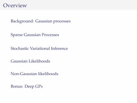
Overview
Background: Gaussian processes
Sparse Gaussian Processes
Stochastic Variational Inference
Gaussian Likelihoods
Non-Gaussian likelihoods
Bonus: Deep GPs
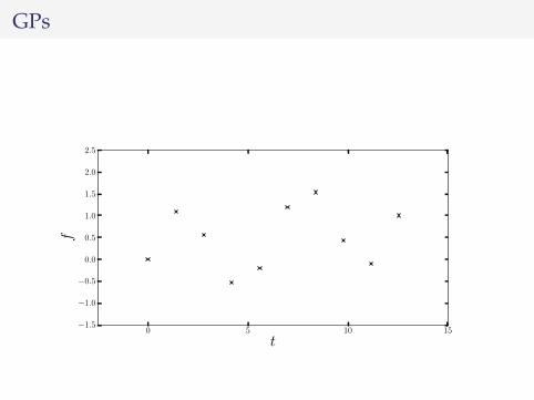
GPs
0 5 10 15
t−1.5
−1.0
−0.5
0.0
0.5
1.0
1.5
2.0
2.5
f

GPs - prior over functions
f ∼ GP(0, k(t, t′))
0 5 10 15
t−4
−3
−2
−1
0
1
2
3
4
f

GPs - posterior over functions
0 5 10 15
t−1.5
−1.0
−0.5
0.0
0.5
1.0
1.5
2.0
2.5
f

GPs - analytical solution
f |y ∼ GP(k(x, x)K−1y, k(x, x′) − k(x, x)K−1k(x, x′)
)
0 5 10 15
t−1.5
−1.0
−0.5
0.0
0.5
1.0
1.5
2.0
2.5
f

What about noise?
Gaussian noise is tractable - additional parameter σn
0 5 10 15
t−1.5
−1.0
−0.5
0.0
0.5
1.0
1.5
2.0
2.5
f

Parameters
−4−3−2−1
01234
−4−3−2−1
01234
0 5 10 15−4−3−2−1
01234
0 5 10 15
Overview
Background: Gaussian processes
Sparse Gaussian Processes
Stochastic Variational Inference
Gaussian Likelihoods
Non-Gaussian likelihoods
Bonus: Deep GPs
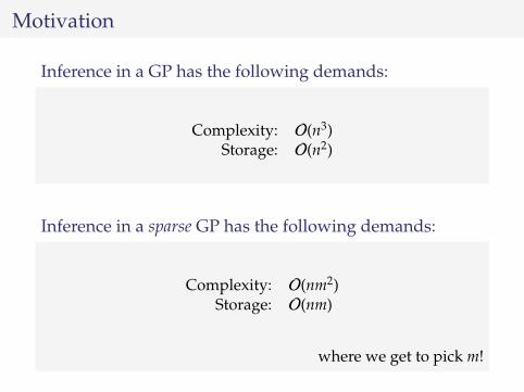
Motivation
Inference in a GP has the following demands:
Complexity: O(n3)Storage: O(n2)
Inference in a sparse GP has the following demands:
Complexity: O(nm2)Storage: O(nm)
where we get to pick m!

Still not good enough!
Big Data
I In parametric models, stochastic optimisation is used.I This allows for application to Big Data.
This work
I Show how to use Stochastic Variational Inference in GPsI Stochastic optimisation scheme: each step requires O(m3)

Overview
Background: Gaussian processes
Sparse Gaussian Processes
Stochastic Variational Inference
Gaussian Likelihoods
Non-Gaussian likelihoods
Bonus: Deep GPs

Incomplete bibliography
(With apologies for 27,000 omissions)
I Csato and Opper, 2002I Seeger 2003, Lawrence and Seeger 2003I Snelson and Ghahramani 2006I Quinonero-Candela and Rasmussen 2005I Titsias 2009I Alvarez and Lawrence 2011

Computational savings
Knn ≈ Qnn = KnmK−1mmKmn
Instead of inverting Knn, we make a low rank (or Nystrom)approximation, and invert Kmm instead.

Information capture
Everything we want to do with a GP involvesmarginalising f
I PredictionsI Marginal likelihoodI Estimating covariance parameters
The posterior of f is the central object. This means invertingKnn.

X, y
input space (X)
function v
alues

X, y
f (x) ∼ GP
input space (X)
function v
alues

X, y
f (x) ∼ GP
p(f) = N (0,Knn)
input space (X)
function v
alues

X, y
f (x) ∼ GP
p(f) = N (0,Knn)
p(f |y,X)
input space (X)
function v
alues

Introducing u
Take and extra M points on the function, u = f (Z).
p(y, f,u) = p(y | f)p(f |u)p(u)

Introducing u

Introducing u
Take and extra M points on the function, u = f (Z).
p(y, f,u) = p(y | f)p(f |u)p(u)
p(y | f) = N(y|f, σ2I
)p(f |u) = N
(f|KnmKmmıu, K
)p(u) = N (u|0,Kmm)

X, y
f (x) ∼ GP
p(f) = N (0,Knn)
p(f |y,X)
Z,up(u) = N (0,Kmm)
input space (X)
function v
alues

X, y
f (x) ∼ GP
p(f) = N (0,Knn)
p(f |y,X)
p(u) = N (0,Kmm)
p(u |y,X)
input space (X)
function v
alues

The alternative posterior
Instead of doing
p(f |y,X) =p(y | f)p(f |X)∫p(y | f)p(f |X)df
We’ll do
p(u |y,Z) =p(y |u)p(u |Z)∫p(y |u)p(u |Z)du
but p(y |u) involves inverting Knn

The alternative posterior
Instead of doing
p(f |y,X) =p(y | f)p(f |X)∫p(y | f)p(f |X)df
We’ll do
p(u |y,Z) =p(y |u)p(u |Z)∫p(y |u)p(u |Z)du
but p(y |u) involves inverting Knn
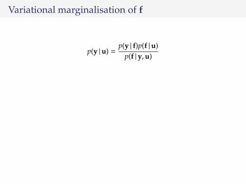
Variational marginalisation of f
p(y |u) =p(y | f)p(f |u)
p(f |y,u)
ln p(y |u) = ln p(y | f) + lnp(f |u)
p(f |y,u)
ln p(y |u) = Ep(f |u)
[ln p(y | f)
]+ Ep(f |u)
[ln
p(f |u)p(f |y,u)
]ln p(y |u) = ln p(y |u) + KL[p(f|u)||p(f |y,u)]
No inversion of Knn required

Variational marginalisation of f
p(y |u) =p(y | f)p(f |u)
p(f |y,u)
ln p(y |u) = ln p(y | f) + lnp(f |u)
p(f |y,u)
ln p(y |u) = Ep(f |u)
[ln p(y | f)
]+ Ep(f |u)
[ln
p(f |u)p(f |y,u)
]ln p(y |u) = ln p(y |u) + KL[p(f|u)||p(f |y,u)]
No inversion of Knn required

Variational marginalisation of f
p(y |u) =p(y | f)p(f |u)
p(f |y,u)
ln p(y |u) = ln p(y | f) + lnp(f |u)
p(f |y,u)
ln p(y |u) = Ep(f |u)
[ln p(y | f)
]+ Ep(f |u)
[ln
p(f |u)p(f |y,u)
]
ln p(y |u) = ln p(y |u) + KL[p(f|u)||p(f |y,u)]
No inversion of Knn required

Variational marginalisation of f
p(y |u) =p(y | f)p(f |u)
p(f |y,u)
ln p(y |u) = ln p(y | f) + lnp(f |u)
p(f |y,u)
ln p(y |u) = Ep(f |u)
[ln p(y | f)
]+ Ep(f |u)
[ln
p(f |u)p(f |y,u)
]ln p(y |u) = ln p(y |u) + KL[p(f|u)||p(f |y,u)]
No inversion of Knn required

An approximate likelihood
p(y |u) =n∏
i=1
N
(yi|k>mnK−1
mmu, σ2)
exp{−
12σ2
(knn − k>mnK−1
mmkmn)}
A straightforward likelihood approximation, and a penaltyterm

Now we can marginalise u
p(u |y,Z) =p(y |u)p(u |Z)∫p(y |u)p(u |Z)du
I Computing the (approximate) posterior costs O(nm2)I We also get a lower bound of the marginal likelihoodI This is the standard variational sparse GP (?).

Overview
Background: Gaussian processes
Sparse Gaussian Processes
Stochastic Variational Inference
Gaussian Likelihoods
Non-Gaussian likelihoods
Bonus: Deep GPs

Stochastic Variational Inference
I Combine the ideas of stochastic optimisation withVariational inference
I example: apply Latent Dirichlet allocation to projectGutenberg
I Can apply variational techniques to Big DataI How could this work in GPs?

But GPs are not factorizing models?
I The variational marginalisation of f introducedfactorisation across the datapoints (conditioned on u)
I Marginalising u re-introdcuced dependencies between thedata
I Solution: a variational treatment of u

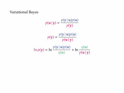
Variational Bayes
p(u |y) =p(y |u)p(u)
p(y)
p(y) =p(y |u)p(u)
p(u |y)
ln p(y) = lnp(y |u)p(u)
q(u)+ ln
q(u)p(u |y)
ln p(y) = Eq(u)
[ln
p(y |u)p(u)q(u)
]+ Eq(u)
[ln
q(u)p(u |y)
]ln p(y) = L + KL
(q(u) ‖ p(u |y)
)

Variational Bayes
p(u |y) =p(y |u)p(u)
p(y)
p(y) =p(y |u)p(u)
p(u |y)
ln p(y) = lnp(y |u)p(u)
q(u)+ ln
q(u)p(u |y)
ln p(y) = Eq(u)
[ln
p(y |u)p(u)q(u)
]+ Eq(u)
[ln
q(u)p(u |y)
]ln p(y) = L + KL
(q(u) ‖ p(u |y)
)
Variational Bayes
p(u |y) =p(y |u)p(u)
p(y)
p(y) =p(y |u)p(u)
p(u |y)
ln p(y) = lnp(y |u)p(u)
q(u)+ ln
q(u)p(u |y)
ln p(y) = Eq(u)
[ln
p(y |u)p(u)q(u)
]+ Eq(u)
[ln
q(u)p(u |y)
]ln p(y) = L + KL
(q(u) ‖ p(u |y)
)

Variational Bayes
p(u |y) =p(y |u)p(u)
p(y)
p(y) =p(y |u)p(u)
p(u |y)
ln p(y) = lnp(y |u)p(u)
q(u)+ ln
q(u)p(u |y)
ln p(y) = Eq(u)
[ln
p(y |u)p(u)q(u)
]+ Eq(u)
[ln
q(u)p(u |y)
]
ln p(y) = L + KL(q(u) ‖ p(u |y)
)

Variational Bayes
p(u |y) =p(y |u)p(u)
p(y)
p(y) =p(y |u)p(u)
p(u |y)
ln p(y) = lnp(y |u)p(u)
q(u)+ ln
q(u)p(u |y)
ln p(y) = Eq(u)
[ln
p(y |u)p(u)q(u)
]+ Eq(u)
[ln
q(u)p(u |y)
]ln p(y) = L + KL
(q(u) ‖ p(u |y)
)

The objective
L = Eq(f)[log p(y | f)] − KL(q(u) ‖ p(u)
)I Tractable for Gaussian likelihoodsI Numerical integration (1D) for intractable likelihoods
(classification)

Optimisation
The variational objective L3 is a function of
I the parameters of the covariance functionI the parameters of q(u)I the inducing inputs, Z
Original strategy: set Z. Take the data in small minibatches,take stochastic gradient steps in the covariance functionparameters, stochastic natural gradient steps in the parametersof q(u).
New strategy: represent S as LL> (unconstrained). Throwm,L,Z,θ at Adagrad.

Optimisation
The variational objective L3 is a function of
I the parameters of the covariance functionI the parameters of q(u)I the inducing inputs, Z
Original strategy: set Z. Take the data in small minibatches,take stochastic gradient steps in the covariance functionparameters, stochastic natural gradient steps in the parametersof q(u).New strategy: represent S as LL> (unconstrained). Throwm,L,Z,θ at Adagrad.

Overview
Background: Gaussian processes
Sparse Gaussian Processes
Stochastic Variational Inference
Gaussian Likelihoods
Non-Gaussian likelihoods
Bonus: Deep GPs


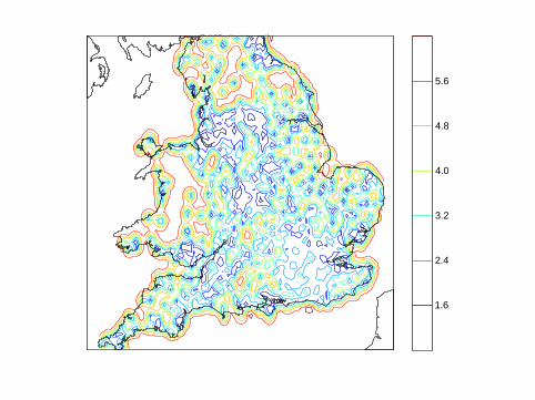
UK apartment prices
I Monthly price paid data for February to October 2012(England and Wales)
I from http://data.gov.uk/dataset/land-registry-monthly-price-paid-data/
I 75,000 entriesI Cross referenced against a postcode database to get
lattitude and longitudeI Regressed the normalised logarithm of the apartment
prices


Airline data
I Flight delays for everycommercial flight in theUSA from January to April2008.
I Average delay was 30minutes.
I We randomly selected800,000 datapoints (wehave limited memory!)
I 700,000 train, 100,000 test
Month
DayOfM
onth
DayOfW
eek
DepTim
e
ArrTim
e
AirTim
e
Distan
ce
PlaneA
ge0.0
0.1
0.2
0.3
0.4
0.5
0.6
0.7
0.8
0.9
Invers
e length
scale
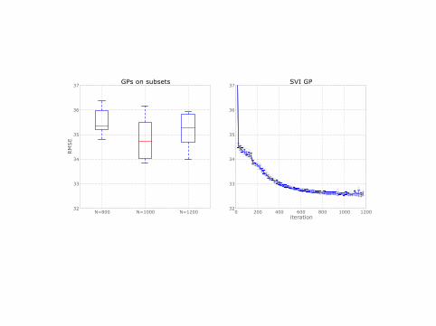
N=800 N=1000 N=120032
33
34
35
36
37
RM
SE
GPs on subsets
0 200 400 600 800 1000 1200iteration
32
33
34
35
36
37SVI GP


Overview
Background: Gaussian processes
Sparse Gaussian Processes
Stochastic Variational Inference
Gaussian Likelihoods
Non-Gaussian likelihoods
Bonus: Deep GPs
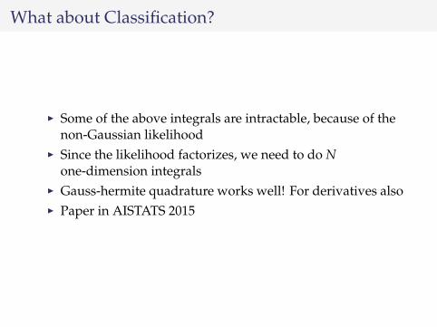
What about Classification?
I Some of the above integrals are intractable, because of thenon-Gaussian likelihood
I Since the likelihood factorizes, we need to do None-dimension integrals
I Gauss-hermite quadrature works well! For derivatives alsoI Paper in AISTATS 2015

Does it work?KLSP
M=4 M=8 M=16 M=32 M=64 Full
MF
GFIT
C
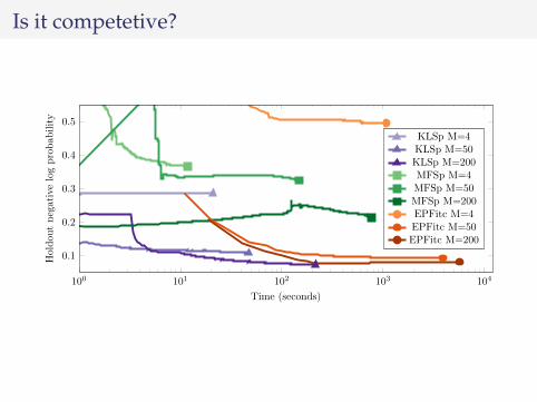
Is it competetive?
100 101 102 103 104
0.1
0.2
0.3
0.4
0.5
Time (seconds)
Holdou
tnegativelogprobab
ility
KLSp M=4KLSp M=50KLSp M=200MFSp M=4MFSp M=50MFSp M=200EPFitc M=4EPFitc M=50EPFitc M=200

Big data?
102 103 104 1050.320.340.360.380.4
error(%
)
102 103 104 1050.6
0.62
0.64
0.66
Time (seconds)
-log
p(y)
Overview
Background: Gaussian processes
Sparse Gaussian Processes
Stochastic Variational Inference
Gaussian Likelihoods
Non-Gaussian likelihoods
Bonus: Deep GPs

Bonus! Deep GPs
Deep models using compound functions:
y = f1( f2(... fn(x)))

xn
h(1)nqu(1)
d
Z0
Z1
h(2)nqu(2)
dZ2
yndu(3)d
d = 1...D1
d = 1...D2
d = 1...Dn = 1...N

000001002003004005006007008009010011012013014015016017018019020021022023024025026027028029030031032033034035036037038039040041042043044045046047048049050051052053054
055056057058059060061062063064065066067068069070071072073074075076077078079080081082083084085086087088089090091092093094095096097098099100101102103104105106107108109
0
0.5
1
000001002003004005006007008009010011012013014015016017018019020021022023024025026027028029030031032033034035036037038039040041042043044045046047048049050051052053054
055056057058059060061062063064065066067068069070071072073074075076077078079080081082083084085086087088089090091092093094095096097098099100101102103104105106107108109
−1 −0.5 0 0.5 1 1.5 2
0
0.5
1

0 5 10 15 20 25 300
5
10
15
20
25
30
35
40
45

0.0 0.2 0.4 0.6 0.8 1.0
1.0
0.5
0.0
0.5
1.0
1.5
2.0
2.5
3.0

1.1 1.0 0.9 0.8 0.7 0.6 0.5 0.430
20
10
0
10
20
30
40
50
60

25 20 15 10 5 0 5 10 15 2030
20
10
0
10
20
30
![K2-ABC: Approximate Bayesian Computation with Kernel ...proceedings.mlr.press/v51/park16.pdf · for models with intractable likelihoods. Originated in population genetics [1], ABC](https://static.fdocuments.net/doc/165x107/5ec5a3d8691079698166a1c0/k2-abc-approximate-bayesian-computation-with-kernel-for-models-with-intractable.jpg)