Scalable and Cost-Effective Model-Based Software Verification and Testing

University of Luxembourg Interdisciplinary Centre for Security, Reliability and Trust Software Verification and Validation Lab (www.svv.lu) May 17th, 2013 University of California, Irvine Lionel Briand, IEEE Fellow FNR PEARL Chair

Luxembourg

•  Small country and population

•  One of the wealthiest in the world

•  Young university (2003) and Ph.D. programs (2007)

•  ICT security and reliability, a national research priority

•  Priorities implemented as interdisciplinary centres

•  International

•  Three official languages: English, French, German

2

SnT Software Verification and Validation Lab

•  SnT centre, Est. 2009: Interdisciplinary, ICT security-reliability-trust

•  180 scientists and Ph.D. candidates, 20 industry partners

•  SVV Lab: Established January 2012, www.svv.lu

•  15 scientists (Research scientists, associates, and PhD candidates)

•  Industry-relevant research on system dependability: security, safety, reliability

•  Four partners: Cetrel, CTIE, Delphi, SES, …

3

Research Paradigm

•  Research informed by practice

•  Well-defined problems in context

•  Realistic evaluation

•  Long term industrial collaborations

4

Acknowledgements

•  Shiva Nejati

•  Mehrdad Sabetzadeh

•  Yvan Labiche

•  Andrea Arcuri

•  Stefano Di Alesio

•  Reza Matinnejad

•  Zohaib Iqbal

•  Shaukat Ali

•  Hadi Hemmati •  Marwa Shousha

•  …

5

“Model-based”?

•  All engineering disciplines rely on abstraction and therefore models

•  In most cases, it is the only way to effectively automate testing or verification

•  Models have many other purposes: Communication, support requirements and design

•  There are many ways to model systems and their environment

•  In a given context, this choice is driven by the application domain, standards and practices, objectives, and skills

6

Models in Software Engineering

•  Model: An abstract and analyzable description of software artifacts, created for a purpose

7

Requirements models Architecture models Behavioural

models Test models

•  Abstract: Details are omitted. Partial representation. Much smaller and simpler than the artifact being modeled.

•  Analyzable: Leads to task automation

Talk Objectives

•  Overview of several years of research

•  Examples, at various levels of details

•  Follows a research paradigm that is uncommon in software engineering research

•  Conducted in collaboration with industry partners in many application domains: Automotive, energy, telecom …

•  Lessons learned regarding scalability and cost-effectiveness

8

9

Objective Function

Search Space

Search Technique

  Search to optimize objective function: Complete or not, deterministic or partly random (stochastic)

  Metaheuristics, constraint solvers

  Scalability: A small part of the search space is traversed

  Model: Guidance to worst case, high risk scenarios across space

  Heuristics: Extensive empirical studies are required

Research Pattern: Models and Search Heuristics

Early Work: Search-Based Schedulability Analysis

L. Briand, Y. Labiche, and M. Shousha, 2003-2006

10

•  Real-time scheduling theory –  Given priorities, execution time, periods (periodic task), minimum

inter-arrival times (aperiodic task), … –  Is a group of (a)periodic tasks schedulable? –  Theory to determine schedulability

•  Independent periodic tasks: Rate Monotonic Algorithm (RMA) •  Aperiodic or dependent tasks: Generalized Completion Time

Theorem (GCTT). •  GCTT assumes

–  aperiodic tasks equivalent to periodic tasks •  periods = minimum inter-arrival times

–  aperiodic tasks ready to start at time zero •  Execution times are estimates

t2t2

t2

t2

0

2

4

6

8

10

12

14

16

18

20

minimum interarrival time: 8

Schedulability Theory

11

A Search-based Solution

•  Goal: Make no assumptions and find near deadline misses as well, identify worst case scenarios

•  Population-based metaheuristic: Genetic Algorithm

•  To automate, based on the system task architecture (UML SPT, MARTE), the derivation of arrival times for task triggering events that maximize the chances of critical deadline misses.

12

Aperiodic tasks

Periodic tasks

System

Event 1

Event 2

+ Genetic Algorithm

=

Arrival times

Event 1

Event 1

Event 2

time

Model as Input

13

UML-MARTE Model (Task architecture)

GA

Scheduler (constraint solver)

• Chromosome • Fitness evaluation

Task priorities …

Estimated execution time, Minimum inter-arrival time, …

Arrival/seeding times

Start times, Pre-emption

Objective Function

•  Focus on one target task at a time

•  Goal: Guide the search towards arrival times causing the greatest delays in the executions of the target task

•  Properties:

–  Handle deadline misses –  Consider all task executions, not just worst case execution

–  Reward task executions so that many good executions do not wind up overshadowing one bad execution

14

Objective Function II

∑=

−=t

jtjt

k

j

deChf1

,,2)(

t: target task kt: maximum number of executions of t e: estimated end time of execution j of target task as determined by scheduler d: deadline of execution j of target task

f

e-d 0

15

Case Study

•  Software Engineering Institute (SEI), Naval Weapons Center and IBM’s Federal Sector Division

•  Hard real-time, realistic avionics application model similar to existing U.S. Navy and Marine aircrafts

•  Eight highest priority tasks deemed schedulable

•  Our findings suggest three of eight tasks produce systematic deadline misses

16

0

0

2

0

0

4

7

0

N/A

N/A

3, 9

N/A

N/A

17, 16, 10, 9

1, 29, 23, 2, 28, 27, 32

N/A

Number of Misses

Value of Misses

Weapon Release

Weapon Release Subtask

Radar Tracking Filter

RWR Contact Management

Data Bus Poll Device

Weapon Aiming

Radar Target Update

Navigation Update

Results

Conclusions

•  We devised a method to generate event seeding times for aperiodic tasks so as identifying deadline miss scenarios based on task design information

•  Near deadline misses as well! (stress testing)

•  Standard modeling notation (UML/SPT/MARTE)

•  No dedicated, additional modeling compared to what is expected when defining a task architecture

•  Scalability: GA runs lasted a few minutes on regular PC

•  Default GA parameters, as recommended in literature, work well

•  Large empirical studies to evaluate the approach (heuristics)

•  Similar work with concurrency analysis: Deadlocks, data races, etc. (Shousha, Briand, Labiche, 2008-2012)

Testing Driven by Environment Modeling

Z. Iqbal, A. Arcuri, L. Briand, 2009-2012

19

•  Three-year project with two industry partners

–  Soft real-time systems: deadlines in order of hundreds of milliseconds

•  Jitter of few milliseconds acceptable

–  Automation of test cases and oracle generation, environment simulation

Tomra – Bottle Recycling Machine WesternGeco – Marine Seismic

Acquisition System

Context'

•  Independent

–  Black-box

•  Behavior driven by environment

–  Environment model

•  Software engineers

•  No use of Matlab/Simulink

•  One model for

–  Environment simulator

–  Test cases and oracles •  UML profile (+ limited use of

MARTE)

Environment Simulator

Test cases

Environment Models

Test oracle

Environment'Modeling'and'Simula4on'

Domain'Model'

Behavior'Model'

•  Test cases are defined by

–  Simulation configuration

–  Environment configuration

•  Environment Configuration

–  Number of instances to be created for each component in the domain model (e.g., the number of sensors)

•  Simulator Configuration

–  Setting of non-deterministic attribute values

•  Test oracle: Environment model error states

–  A successful test case is one which leads the environment into an error state

Test'Cases'

•  Bring the system state to an error state by searching for appropriate values for non-deterministic environment attributes

•  Search heuristics are based on fitness functions assessing how “close” is the current state to an error state

•  Different metaheuristics: Genetic algorithm, (1+1) EA

•  Defining the fitness function based on model information was highly complex: OCL constraints, combination of many heuristics

•  Industrial case study and artificial examples showed the heuristic was effective

–  (1+1) EA better than GA

25

Search'Objec4ves'and'Heuris4cs'

•  Evaluates how “good” the simulator configurations are

•  Can only be decided after the execution of a test case

•  Decided based on heuristics: How close was the test case to …

26

•  Approach Level •  reach an error state?

•  Branch Distance •  solve the guard on a

branch leading to an error state?

•  defined search heuristics for OCL expressions*

•  Time Distance •  take a time transition that

leads to an error state?

Basic'Ideas'about'the'Fitness'Func4on'

* S. Ali, M.Z. Iqbal, A. Arcuri, L. Briand, "Generating Test Data from OCL Constraints with Search Techniques", forthcoming in IEEE Transactions on Software Engineering

Constraint Optimization to Verify CPU Usage

S. Nejati, S. Di Alesio, M. Sabetzadeh, L. Briand, 2012

27

System: fire/gas detection and emergency shutdown

28

Drivers (Software-Hardware Interface)

Control Modules Alarm Devices (Hardware)

Multicore Archt.

Real Time Operating System

Safety Drivers May Overload the CPU

•  Drivers need to bridge the timing gaps between SW and HW

•  SIL 3

•  Drivers have flexible design

•  Parallel threads communicating in an asynchronous way

•  Period and watchdog threads

•  Drivers are subject to real-time constraints to make sure they do not overuse the CPU time, e.g., “The processor spare-time should not be less than 80% at any time”

•  Determine how many driver instances to deploy on a CPU

29

Drivers (Software-Hardware Interface)

30

Pull Data IODispatch Push Data

Periodic Periodic WatchDog

Delay (offset)

Small Delay

Large Delay

T2 consumes a lot of CPU time

T2 may blockT1 and/or T3

T1 T3 T2

Deadline misses

CPU overload

Communication protocol with configurable parameters

Processing control data

Sending HW commands

I/O Driver

Safety standards

To achieve SIL levels 3-4, Stress Testing is “Highly Recommended”

IEC 61508 is a Safety Standard including guidelines for Performance Testing

iec.ch

31

Search Objective

•  Stress test cases: Values for environment-dependent parameters of the embedded software, e.g., the size of time delays used in software to synchronize with hardware devices or to receive feedback from the hardware devices.

•  Goal: select delays to maximize the use of the CPU while satisfying design constraints.

32

General Approach: Modeling and Optimization

Constraint Programming

Modeling

Constraint Program

Stress Test Cases (Delay values leading to worst

case CPU time usage)

Performance Requirements

(objective functions)

System design and platform Model (UML/MARTE)

INPUT

OUTPUT

CP Engine (COMET)

INPUT

Information Requirements

34

Scheduler

Activity

- preemptive : bool

- min duration(min_d) :int- max duration (max_d) :int- delay :int

Processing Unit- number of cores :int

Global Clock- time : int

Thread

1.. *

Scheduling Policy

uses

schedules

1.. *

1

*11

*

*

Data dependency ( )

- priority :int- period (p) :int- min inter-arrival time (min_ia) :int- max inter-arrival time (max_ia) :int

ordered

Asynch

0..1*

*

*

temporal precedence( )

- Start()- Finish()- Wait()- Sleep()- Resume()- Trigger()

Buffer- size : int0..11.. *- access()

�t

triggers

Computing Platform Embedded Software Appallocated

11

**

Synch

uses1.. *

0..1

1 *

*

runs *

MARTE: Augmented Sequence Diagrams

35

IOTask Push Data MailBox

Some abstractions are design choices: delays, priorities…

Pull Data

scan

Some others depend on the environment: arrival times…

Thread

Buffer

Activity

delay

duration

deadline

COMET input language Design properties include: threads, priorities, activities, durations… Preemptions at regular time periods (quanta) Assume negligible context switching time compared to time quantum Platform and design properties are constants in our Constraint Program

Platform and Design Properties modeled in UML are provided as input in our Constraint

Program // 1) Input: Time and Concurrency information int c = ...; // #Cores int n = ...; range J = 0..n-1; // #Threads int priority[J] = ...; // Priorities // ... // 2) Output: Scheduling variables dvar int arrival_time[a in A] in T;

// Actual arrival times dvar int start[a in A] in est[a]..lst[a];

// Actual start times dvar int end[a in A] in eet[a]..let[a];

// Actual end times // ... // 3) Objective function: Performance Requirement maximize

sum(a in A)(maxl(0, minl(1, deadline_miss[a]))); // Deadline misses function // 4) Constraints: Scheduling policy subject to {

forall(a in A) { wf4: start[a] <= end[a];

// Threads should end after their start time // ...

Threads Properties which can be tuned during testing are the output of our Constraint Program

Tunable Parameters may include design and real time properties Tunable Parameters are variables in our Constraint Program Some tunable parameters are the basis for the definition to stress test cases (e.g., delays), others are results from scheduling

// 1) Input: Time and Concurrency information int c = ...; // #Cores int n = ...; range J = 0..n-1; // #Threads int priority[J] = ...; // Priorities // ... // 2) Output: Scheduling variables dvar int arrival_time[a in A] in T;

// Actual arrival times dvar int start[a in A] in est[a]..lst[a];

// Actual start times dvar int end[a in A] in eet[a]..let[a];

// Actual end times // ... // 3) Objective function: Performance Requirement maximize

sum(a in A)(maxl(0, minl(1, deadline_miss[a]))); // Deadline misses function // 4) Constraints: Scheduling policy subject to {

forall(a in A) { wf4: start[a] <= end[a];

// Threads should end after their start time // ...

The Performance Requirement is modeled as an objective function to maximize

We focus on objective functions for CPU Usage here Each objective function models a specific performance requirement Testing a different performance requirements only requires to change the objective function (constraints)

// 1) Input: Time and Concurrency information int c = ...; // #Cores int n = ...; range J = 0..n-1; // #Threads int priority[J] = ...; // Priorities // ... // 2) Output: Scheduling variables dvar int arrival_time[a in A] in T;

// Actual arrival times dvar int start[a in A] in est[a]..lst[a];

// Actual start times dvar int end[a in A] in eet[a]..let[a];

// Actual end times // ... // 3) Objective function: Performance Requirement maximize

sum(a in A)(maxl(0, minl(1, deadline_miss[a]))); // Deadline misses function // 4) Constraints: Scheduling policy subject to {

forall(a in A) { wf4: start[a] <= end[a];

// Threads should end after their start time // ...

Constraints express relationships between constants and variables Constraints are independent and can be modified to fit different platforms, for example scheduling algorithm

The Platform scheduler and properties are modeled through a set of constraints

// 1) Input: Time and Concurrency information int c = ...; // #Cores int n = ...; range J = 0..n-1; // #Threads int priority[J] = ...; // Priorities // ... // 2) Output: Scheduling variables dvar int arrival_time[a in A] in T;

// Actual arrival times dvar int start[a in A] in est[a]..lst[a];

// Actual start times dvar int end[a in A] in eet[a]..let[a];

// Actual end times // ... // 3) Objective function: Performance Requirement maximize

sum(a in A)(maxl(0, minl(1, deadline_miss[a]))); // Deadline misses function // 4) Constraints: Scheduling policy subject to {

forall(a in A) { wf4: start[a] <= end[a];

// Threads should end after their start time // ...

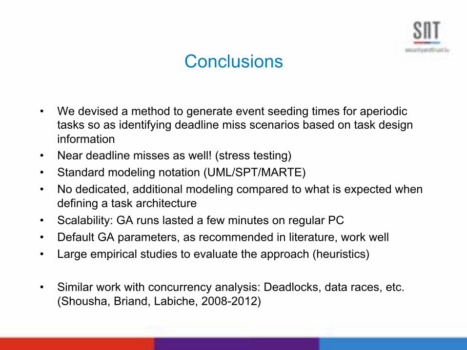
We run an experiment with real data and two different objective functions

But optimal solutions were found shortly after the search started, even if the search took a much more time to terminate

It took a significant amount of time for the search to terminate

Case Study (Driver)

40

(Time) (Time)

Max: 50%Max: 50%

Max:550 ms

Max:550 ms

termination time termination timetermination time termination time

(% for cpu usage,ms for makespan)

(Val

ue)

(Val

ue)

(% for cpu usage,ms for makespan)

Fig. 5. The result of maximizing fmakespan and fusage (Section 4) for both parallel and non-parallel COMET implementations.

usage requirements. To identify the suspicious hardware configurations, however, theanalysis provided in this paper is necessary because the hardware configurations affectthe delay times of the IO drivers activities, and subsequently, the CPU usage estimates.

For example, the size of the delay time at step 3 of the data transfer scenario inFigure 1(b) can heavily impact the CPU usage. Specifically, the delay time cannot beso small that IODispatch (Figure 1(a)) keeps the CPU busy for so long that it exceedsthe given CPU usage requirement. Neither can the delay be too large, because thenpullData, which is periodic, may miss its deadline. Specifically it may quickly fill upthe Message Box 1 buffer, which in turn causes pullData to be blocked and waitingfor IODispatch to empty Message Box 1, which is now very slow due to a large delaytime. As a result, pullData may not be able to terminate before its next scan arrival.

To derive stress test cases based on the delay times of the activities, in our formula-tion in Figure 4, we specify delay as an output variable whose value is bounded withina range. The search then varies the values of these variables to maximize fmakespan andfusage . Those combinations that maximize our objective functions are more likely tostress the system to the extent that the CPU usage requirements are violated.

To perform the above experiment, we implemented the constraint optimization for-mulation in Figure 4 in COMET Version 2.1.0 [7]. We further used the native supportof COMET for parallel programming to create a distributed version of our COMET im-plementation that divides the search work-load among different cores. To perform theexperiment, we varied the observation time T from 1s to a few seconds and set thequantum time (i.e., the minimum time step that a scheduler may preempt activities) to10 ms. The input model included eight activities belonging to three parallel threads.

Figure 5 shows the result of our experiment, maximizing fmakespan and fusage forboth parallel and non-parallel COMET implementations. In both diagrams, the X-axisshows the time, and the Y-axis shows the size of fmakespan in ms, and the percentage forfusage . In our experiment, we used a complete (exhaustive) constraint solver of COMET,and ran it on a MacBook Pro with a 2.0 Ghz quad-core Intel Core i7 with 8GB RAM.As shown in the figure, the search terminated in both cases: after around 14 hours forthe non-parallel version, and after around 2 hours and 55 min for the parallel version.The maximum computed values are: 50% for fusage , and 550 ms for fmakespan . In thenon-parallel case, the maximum result was computed after around 1 hour and 10 minfor fmakespan , and 1 hour and 13 min for fusage . No higher value was found in theremainder of the search which took more than 14 hours in total. In the parallel case,

13

Conclusions

•  We re-express test case generation for CPU usage requirements as a constraint optimization problem

•  Approach: –  A conceptual model for time abstractions –  Mapping to MARTE –  A constraint optimization formulation of

the problem –  Application of the approach to a real case

study (albeit small)

•  Using a constraint solver does not seem to scale to large numbers of threads

•  Currently continues this work with Delphi using metaheuristic search: 430 tasks, powertrain systems, AUTOSAR

41

Testing Closed Loop Controllers

R. Matinnejad, S. Nejati, L. Briand, T. Bruckmann, C. Poull, 2013

42

Complexity'and'amount'of'soDware'used'on'vehicles’''Electronic'Control'Units'(ECUs)'grow'rapidly''

More functions

Comfort and variety

Safety and reliability

Faster time-to-market

Less fuel consumption

Greenhouse gas emission laws

43

Three'major'soDware'development'stages'in''the'automo4ve'domain'

44

Major'Challenges'in'MiLKSiLKHiL'Tes4ng''

•  Manual test case generation

•  Complex functions at MiL, and large and integrated software/embedded systems at HiL

•  Lack of precise requirements and testing Objectives

•  Hard to interpret the testing results 45

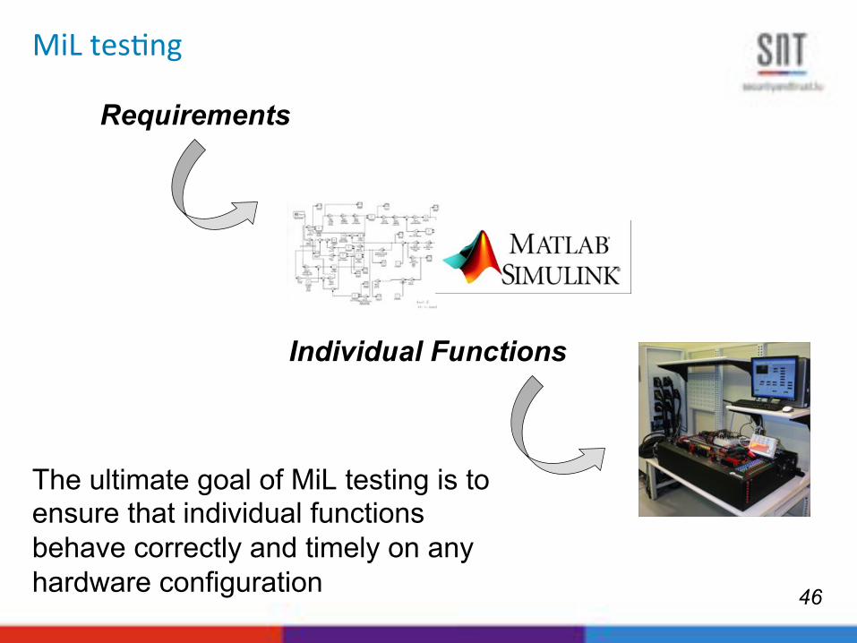
MiL'tes4ng'

Requirements

The ultimate goal of MiL testing is to ensure that individual functions behave correctly and timely on any hardware configuration

Individual Functions

46

Main'differences'between'automo4ve'func4on''tes4ng'and'general'soDware'tes4ng'

•  Continuous behaviour

•  Time matters a lot

•  Several configurations –  Huge number of detailed physical measures/ranges/

thresholds captured by calibration values

47

A'Taxonomy'of'Automo4ve'Func4ons'

Controlling Computation

State-Based Continuous Transforming Calculating

unit convertors calculating positions, duty cycles, etc

State machine controllers

Closed-loop controllers (PID)

Different testing strategies are required for different types of functions

48

Controller Plant Model and its Requirements

Plant Model

Controller(SUT)

Desired value Error

Actual value

System output+-

=<

~= 0>=

time time time

Des

ired

Valu

e &

Actu

al V

alue

Desired ValueActual Value

(a) (b) (c)Liveness Smoothness Responsiveness

x

y

z

v

w

49

50

Types'of'Requirements'

SBPC function shall guarantee that the flap will move to and will stabilize at its desired position within xx ms. Further, the flap shall reach within yy% of its desired position within zz ms. In addition, after reaching vv% close to the desired position, the flap shall not jump to a position more than ww% away from its desired position.

(1) functional/liveness (2) responsiveness/performance

(3) smoothness/safety

xx

zz

yy

<ww

50

51

Search'Elements'

•  Search:

•  Inputs: Initial and desired values, configuration parameters •  (1+1) EA

•  Search Objective:

•  Example requirement that we want to test: liveness

  |Desired - Actual(final)|~= 0

For each set of inputs, we evaluate the objective function over the resulting simulation graphs:

•  Result:

•  worst case scenarios or values to the input variables that are more likely to break the requirement at MiL level

•  stress test cases based on actual hardware (HiL)

51

MiL-Testing of Continuous Controllers

Exploration+Controller-plant model

Objective Functions

Overview Diagram

Test Scenarios

List of Regions Local SearchDomain

Expert

time

Desired ValueActual Value

0 1 20.0

0.1

0.2

0.3

0.4

0.5

0.6

0.7

0.8

0.9

1.0

Initial Desired

Final Desired

52

Generated Heatmap Diagrams

(a) Liveness (b) Smoothness

(c) Responsiveness

53

Random Search vs. (1+1)EA Example with Responsiveness Analysis

Random (1+1) EA

54

•  We found much worse scenarios during MiL testing than our partner had found so far

•  They are running them at the HiL level, where testing is much more expensive: MiL results -> test selection for HiL

•  On average, the results of the single-state search showed significant improvements over the result of the exploration algorithm

•  Configuration parameters?

•  Need more exploitative or explorative search algorithms in different subregions

Conclusions'

i.e., 31s. Hence, the horizontal axis of the diagrams in Figure 8 shows the number ofiterations instead of the computation time. In addition, we start both random search and(1+1) EA from the same initial point, i.e., the worst case from the exploration step.

Overall in all the regions, (1+1) EA eventually reaches its plateau at a value higherthan the random search plateau value. Further, (1+1) EA is more deterministic than ran-dom, i.e., the distribution of (1+1) EA has a smaller variance than that of random search,especially when reaching the plateau (see Figure 8). In some regions (e.g., Figure 8(d)),however, random reaches its plateau slightly faster than (1+1) EA, while in some otherregions (e.g. Figure 8(a)), (1+1) EA is faster. We will discuss the relationship betweenthe region landscape and the performance of (1+1) EA in RQ3.RQ3. We drew the landscape for the 11 regions in our experiment. For example, Fig-ure 9 shows the landscape for two selected regions in Figures 7(a) and 7(b). Specifically,Figure 9(a) shows the landscape for the region in Figure 7(b) where (1+1) EA is fasterthan random, and Figure 9(b) shows the landscape for the region in Figure 7(a) where(1+1) EA is slower than random search.

0.30

0.31

0.32

0.33

0.34

0.35

0.36

0.37

0.38

0.39

0.40

0.70 0.71 0.72 0.73 0.74 0.75 0.76 0.77 0.78 0.79 0.800.10

0.11

0.12

0.13

0.14

0.15

0.16

0.17

0.18

0.19

0.20

0.90 0.91 0.92 0.93 0.94 0.95 0.96 0.97 0.98 0.99 1.00

(a) (b)

Fig. 9. Diagrams representing the landscape for two representative HeatMap regions: (a) Land-scape for the region in Figure 7(b). (b) Landscape for the region in Figure 7(a).

Our observations show that the regions surrounded mostly by dark shaded regionstypically have a clear gradient between the initial point of the search and the worst casepoint (see e.g., Figure 9(a)). However, dark regions located in a generally light shadedarea have a noisier shape with several local optimum (see e.g., Figure 9(b)). It is knownthat for regions like Figure 9(a), exploitative search works best, while for those like Fig-ure 9(b), explorative search is most suitable [10]. This is confirmed in our work wherefor Figure 9(a), our exploitative search, i.e., (1+1) EA with � = 0.01, is faster and moreeffective than random search, whereas for Figure 9(b), our search is slower than randomsearch. We applied a more explorative version of (1+1) EA where we let � = 0.03 to theregion in Figure 9(b). The result (Figure 10) shows that the more explorative (1+1) EAis now both faster and more effective than random search. We conjecture that, from theHeatMap diagrams, we can predict which search algorithm to use for the single-statesearch step. Specifically, for dark regions surrounded by dark shaded areas, we suggestan exploitative (1+1) EA (e.g., � = 0.01), while for dark regions located in light shadedareas, we recommend a more explorative (1+1) EA (e.g., � = 0.03).

6 Related WorkTesting continuous control systems presents a number of challenges, and is not yet sup-ported by existing tools and techniques [4, 1, 3]. The modeling languages that have been

13

55

Minimizing CPU Time Shortage Risks in Integrated Embedded Software

S. Nejati, M. Adedjouma

L. Briand, T. Bruckmann, C. Poull, 2013

56

Today’s'cars'rely'on'integrated'systems'

•  Modular and independent development

•  Huge opportunities for division of labor and outsourcing

•  Need for reliable and effective integration processes

57

An'overview'of'an'integra4on'process'in'the''automo4ve'domain'

AUTOSAR Models sw runnables

sw runnables AUTOSAR Models

Glue

58

AUTOSAR'captures'the'4ming'proper4es'of'the''Runnables'and'their'data'dependencies''''

Component Type

Port

Runnable

OS Task

- period

Internal behaviour

- priority- cycle

DataRead/WriteAccess

InterfaceDataSend/

ReceivePoint

1 *1

*

1 1

11

Autosar Models

Autosar Models

sw runnables

sw runnables

OEM

Supplier

Glue Code

OS

Integrated System

Fig. 1. Overview of the Integration Process.

with a lower bound of 2.05ms on the maximum CPU usage.Our experiments show that our algorithms can automaticallygenerate offsets such that the maximum CPU usage is as low as2.14ms. Such a low limit on the maximum CPU usage had notbeen previously found by the offset computation algorithmsdeveloped at our partner company, Delphi. In addition, ourapproach achieves limits on the maximum CPU usage that aresignificantly lower than those found by a random strategy, thatis used as a baseline of comparison. Finally, our approach isnot slower than the baseline strategy.

II. INTEGRATION PROCESS IN THE AUTOMOTIVE DOMAIN

The software components used on modern vehicles’ Elec-tronic Control Units (ECUs) are rarely developed fully by indi-vidual ECU suppliers. Rather this kind of development is typ-ically distributed between suppliers and car makers (OEMs).This is because OEMs increasingly tend to develop their owncontrol algorithms as well as basic software components toensure optimal software performance for their equipment andplatforms. These components are often treated as proprietarytrade secrets where their executables, i.e., runnables, are onlycommunicated with the ECU suppliers. Hence, the suppliersare often left with the complex task of integrating the third-party runnables with the remaining application and basicsoftware components, and finally deploying the result on theECU hardware. In the end, the suppliers are solely responsiblefor the proper functioning and reliability of the ECUs.

In order to overcome the integration challenges, the auto-motive companies have worked together to develop a stan-dard basis for collaboration and communication called AU-Tomotive Open System ARchitecture (AUTOSAR) [13]. Today,AUTOSAR has become a de-facto open industry standard forautomotive architecture, enabling the modularity and transfer-ability of control functions implemented as runnables.

Figure 1 shows an overview of the integration processtypically followed in the automotive industry. As shown inthe figure, both suppliers and OEMs provide their softwarerunnables (executables) along with AUTOSAR descriptionsfor these runnables. The AUTOSAR descriptions are then usedto automatically generate glue code whose main function isto glue together the runnables and coordinate their commu-nication and their execution on an Operating System (OS).The glue code specifically uses the AUTOSAR informationabout the timing properties of the runnables and their datadependency relations. Figure 2 represents the AUTOSARconcepts that are used to generate the glue code. Note thatFigure 2 is a greatly simplified fragment of the original

Component Type

Port

Runnable

OS Task

- period

Internal behaviour

- priority- cycle

DataRead/WriteAccess

InterfaceDataSend/

ReceivePoint

1 *1

*

1 1

11

Fig. 2. AUTOSAR concepts capturing the timing properties of the runnablesand the data dependencies between them.

/* Declarations for variables, runnables, and dependencies */. . ./* Initializations, constructors and local functions */. . ./* Executing runnables */Task o1() { /* cycle o1 = 5 ms */

if ( (timer mod r1.period) == 0) do /* timer mod 10 == 0 */execute runnable r1

if ( (timer mod r2.period) == 0) do /* timer mod 20 == 0 */execute runnable r2

if ( (timer mod r3.period) == 0) do /* timer mod 100 == 0 */execute runnable r3

. . .}Task o2() {

. . .Fig. 3. Simplified structure of the glue code in Figure 1.

AUTOSAR metamodel [13]. In AUTOSAR, runnables are theatomic units of computation. They can be viewed as concur-rent and communicating threads. In automotive applications,there are typically many more runnables than the maximumnumber of tasks allowed by automotive operating systemssuch as OSEK/VDX or AUTOSAR OS [5]. For this reason,runnables are typically grouped together and scheduled withina sequencer/dispatcher task called OS task (see Figure 2).The partitioning of the runnables and the assignment of thepartitions into different OS tasks is done statically by thesuppliers [5]. Each OS task has a cycle that specifies howoften it is invoked by OS, and a priority which determineswhether its execution can be preempted by another OS task.Each runnable has a period that determines the frequency of itsexecution. The period, further, indicates a deadline by whichthe runnable has to complete its execution. Since runnables areinvoked by their corresponding OS tasks, their periods mustbe divisible by the cycle of their corresponding OS task.

In AUTOSAR, a set of runnables that collectively de-fine a behavior of a component are referred to as aninternal behaviour of that component. Components haveports through which they communicate with one another.The communications between components are implementedvia runnables, and represented by DataRead/WriteAccess, orDataSend/ReceivePoint in Figure 2. According to AUTOSAR,DataRead/WriteAccess indicates a non-blocking mode of com-munication, while DataSend/ReceivePoint refers to a block-ing communication [13]. Both communications can be eithersynchronous or asynchronous. In our work, we refer to bothof these two ways of communications as a data depen-dency between runnables. Data dependency relations betweenrunnables are important because they indicate if the runnablesneed to synchronize with one another, and if so, in what orderthey should run to properly synchronize.

Figure 3 illustrates a simplified overview of the structure ofthe glue code in Figure 1. Given an AUTOSAR description,

Runnables Glue Code:

59

60

CPU'Time'Shortage'in'Integrated'Embedded''SoDware'

•  Challenge –  Many OS tasks and their many runnables run within a limited

available CPU time •  The execution time of the runnables may exceed the OS cycles

•  Our goal –  Reducing the maximum CPU time used per time slot to be

able to •  Minimize the hardware cost •  Enable addition of new functions incrementally •  Reduce the possibility of overloading the CPU in practice

5ms 10ms 15ms 20ms 25ms 30ms 35ms 40ms

✗

5ms 10ms 15ms 20ms 25ms 30ms 35ms 40ms ✔

(a)

(b)

Fig. 4. Two possible CPU time usage simulations for an OS task with a 5mscycle: (a) Usage with bursts, and (b) Desirable usage.

its corresponding glue code starts by a set of declarationsand definitions for components, runnables, ports, etc. It thenincludes the initialization part followed by the execution part.In the execution part, there is one routine for each OS task.These routines are called by the scheduler of the underlyingOS in every cycle of their corresponding task. Inside eachOS task routine, the runnables related to that OS task arecalled based on their period. For example, in Figure 3, weassume that the cycle of the task o1 is 5ms, and the periodof the runnables r1, r2, and r3 are 10ms, 20ms and 100ms,respectively. The value of timer is the global system time. Sincethe cycle of o1 is 5, the value of timer in the Task o1() routineis always a multiple of 5. Runnables r1, r2 and r3 are thencalled whenever the value of timer is zero, or is divisible bythe period of r1, r2 and r3, respectively.

Although AUTOSAR provides a standard means for OEMsand suppliers to exchange their software, and essentiallyenables the process in Figure 1, the automotive integrationprocess still remains complex and erroneous. A major inte-gration challenge is to minimize the risk of CPU shortagewhile running the integrated system in Figure 1. Specifically,consider an OS task with a 5ms cycle. Figure 4 shows twopossible CPU time usage simulations of this task over eighttime slots between 0 to 40ms. In Figure 4(a), there are burstsof high CPU usage at two time slots at 0ms and 35ms, whilethe CPU usage simulation in Figure 4(b) is more stable anddoes not include any bursts. In both simulations, the totalCPU usage is the same, but the distribution of the CPU usageover time slots is different. The simulation in Figure 4(b) ismore desirable because: (1) It minimizes the hardware costsby lowering the maximum required CPU time. (2) It facilitatesthe assignment of new runnables to an OS task, and hence,enables the addition of new functions as it is typically done inthe incremental design of car manufacturers. (3) It reduces thepossibility of overloading CPU as the CPU time usage is lesslikely to exceed the OS task cycle (i.e., 5ms) in any time slot.Ideally, a CPU usage simulation is desirable if in each timeslot, there is a sufficiently large safety margin of unused CPUtime. Due to inaccuracies in estimating runnables’ executiontimes, it is expected that the unused margin shrinks when thesystem runs in a real car. Hence, the larger is this margin, thelower is the probability of exceeding the limit in practice.

In this paper, we study the problem of minimizing burstsof CPU time usage for a software system composed of alarge number of concurrent runnables. A known strategy toeliminate high CPU usage bursts is to shift the start time(offset) of runnables, i.e., to insert a delay prior to the start ofthe execution of runnables [5]. Offsets of the runnables mustsatisfy three constraints: C1. The offset values should not lead

to deadline misses, i.e., they should not cause the runnables torun passed their periods. C2. Since the runnables are invokedby OS tasks, the offset values of each runnable should bedivisible by the OS task cycle related to that runnable. C3. Theoffset values should not interfere with data dependency andsynchronization relations between runnables. For example,suppose runnables r1 and r2 have to execute in the same timeslot because they need to synchronize. The offset values of r1and r2 should be chosen such that they still run in the sametime slot after being shifted by their offsets.

There are four important context factors that are in line withAUTOSAR [13], and have influenced our work:

CF1. The runnables are not memory-bound, i.e., the CPUtime is not significantly affected by the low-bound memoryallocation activities such as transferring data in and out ofthe disk and garbage collection. Hence, our analysis of CPUtime usage is not affected by constraints related to memoryresources (see Section III-B).

CF2. The runnables are Offset-free [4], that is the offset ofa runnable can be freely chosen as long as it does not violatethe timing constraints C1-C3 (see Section III-B).

CF3. The runnables assigned to different OS tasks areindependent in the sense that they do not communicate withone another and do not share memory. Hence, the CPU timeused by an OS task during each cycle is not affected by otherOS tasks running concurrently. Our analysis in this paper,therefore, focuses on individual OS tasks.

CF4. The execution times of the runnables are remarkablysmaller than the runnables’ periods and the OS task cycles.Typical OS task cycles are around 1ms to 5ms. The runnables’periods are typically between 10ms to 1s, while the runnables’execution times are between 10ns = 10�5ms to 0.2ms.

Our goal is to compute offsets for runnables such that theCPU usage is minimized, and further, the timing constraints,C1-C3, discussed earlier above hold. This requires solvinga constraint-based optimization problem, and can be done inthree ways: (1) Attempting to predict optimal offsets in a de-terministic way, e.g., algorithms based on real-time schedulingtheory [6]. In general, these algorithms explore a very smallpart of the search space, i.e., worst/best case situations only(see Section V for a discussion). (2) Formulating the problemas a (symbolic) constraint model and applying a systematicconstraint solver [14], [15]. Due to assumption CF4 above,the search space in our problem is too large, resulting ina huge constraint model that does not fit in memory (seeSection V for more details). (3) Using metaheuristic search-based techniques [9]. These techniques are part of the generalclass of stochastic optimization algorithms which employsome degree of randomness to find optimal (or as optimalas possible) solutions to hard problems. These approaches areapplied to a wide range of problems, and are used in this paper.

III. SEARCH-BASED CPU USAGE MINIMIZATION

In this section, we describe our search-based technique forCPU usage minimization. We first define a notation for ourproblem in Section III-A. We formalize the timing constraints,

60

61

We#minimize#the#maximum#CPU#usage#using#runnables##offsets#(delay#:mes)#

5ms 10ms 15ms 20ms 25ms 30ms 35ms 40ms

5ms 10ms 15ms 20ms 25ms 30ms 35ms 40ms ✗

✔

Inserting runnables’ offsets

Offsets have to be chosen such that the maximum CPU usage per time slot is minimized, and further,

the runnables respect their period the runnables respect the OS cycles the runnnables satisfy their synchronization constraints

61

62

Meta'heuris4c'search''algorithms'

Case Study: an automotive software system with 430 runnables

Running the system without offsets

Simulation for the runnables in our case study andcorresponding to the lowest max CPU usage found by HC

5.34 ms

Our optimized offset assignment

2.13 ms

-  The objective function is the max CPU usage of a 2s-simulation of runnables -  The search modifies one offset at a time, and updates other offsets only if

timing constraints are violated -  Single-state search algorithms for discrete spaces (HC, Tabu) -  Used restart option to make them more explorative

62

63

Comparing'different'search'algorithms''

(ms)

(s)

Best CPU usage

Time to find Best CPU usage

63

64

Comparing'our'best'search'algorithm'with'Random''search'

(a) (b) (c)(a)

Lowest max CPU usage values computed by HC within 70 msover 100 different runs

Lowest max CPU usage values computed by Random within 70 ms over 100 different runs

Comparing average behavior of Random and HC in computinglowest max CPU usage values within 70 s and over 100 different runs

64

65

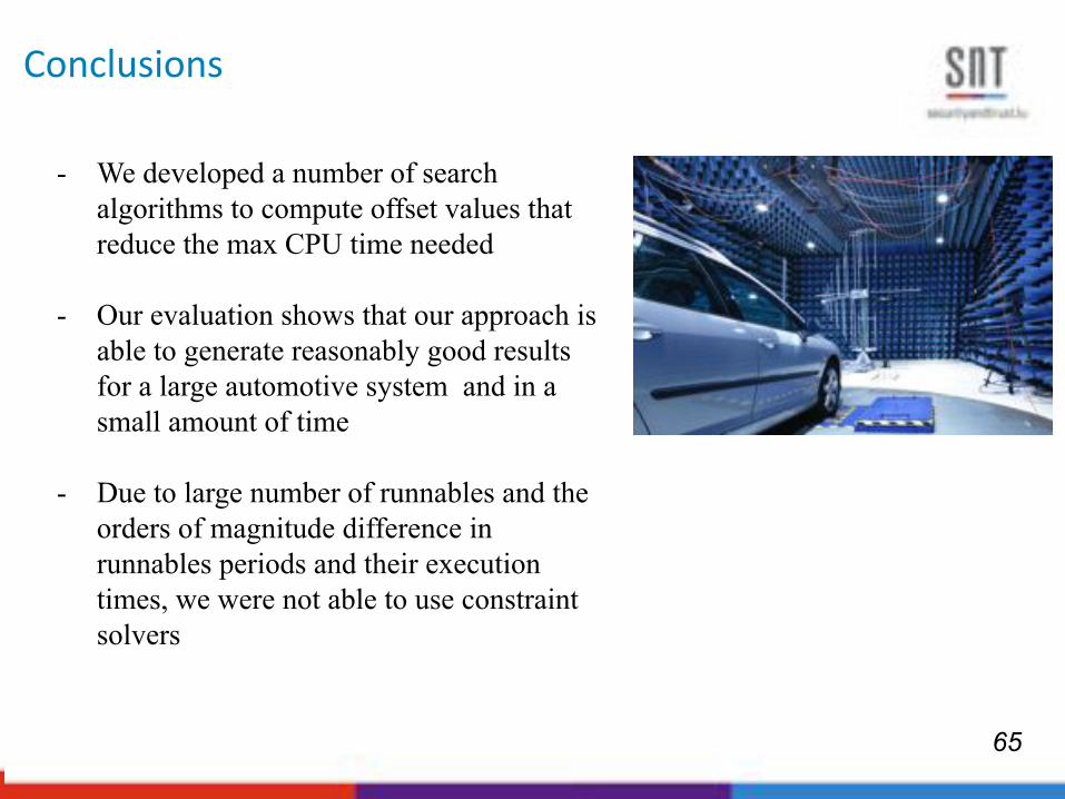
Conclusions'

-  We developed a number of search algorithms to compute offset values that reduce the max CPU time needed

-  Our evaluation shows that our approach is able to generate reasonably good results for a large automotive system and in a small amount of time

-  Due to large number of runnables and the orders of magnitude difference in runnables periods and their execution times, we were not able to use constraint solvers

65

MDE Projects Overview (< 5 years)

66

Company Domain Objective Notation Automation

ABB Robot controller Testing UML Model traversal for coverage criteria

Cisco Video conference Testing (robustness) UML profile Metaheuristic

Kongsberg Maritime Fire and gas safety control system

Certification SysML + req traceability

Slicing algorithm

Kongsberg Maritime Oil&gas, safety critical drivers

CPU usage analysis UML+MARTE Constraint Solver

FMC Subsea system Automated configuration

UML profile Constraint solver

WesternGeco Marine seismic acquisition

Testing UML profile + MARTE Metaheuristic

DNV Marine and Energy, certification body

Compliance with safety standards

UML profile Constraint verification

SES Satellite operator Testing UML profile Metaheuristic

Delphi Automotive systems Testing (safety+performance)

Matlab/Simulink Metaheuristic

Lux. Tax department Legal & financial Legal Req. QA & testing

Under investigation Under investigation

Conclusions I

•  Models

–  UML profiles, MARTE, SysML, Matlab/Simulink, AUTOSAR

–  Never UML only: always some tailoring required

–  Always a specific modeling methodology, i.e., how to use the notation => semantics

–  Driven by

•  Information that is needed to guide automation, e.g., search, optimization

•  Appropriate level of abstraction: scalability, cost-effectiveness

•  Test/Verification objectives

•  Current modeling practices and skills

•  Reliance on standards

–  Modeling requirements must be “reasonable”, achievable, cost-effective for engineers

67

Conclusions II

•  Automation

–  Many testing and verification problems can be re-expressed as a search/optimization problem

–  Search-based software engineering: Enabling automation for hard problems

–  But limited, though changing, applications to model-driven engineering

–  Models are needed to guide search and optimization

–  Many search techniques: Search algorithm, fitness function …

–  It is not easy to choose which one to use for a given problem –  Empirical studies

–  Promising results, scalability (incomplete search)

68

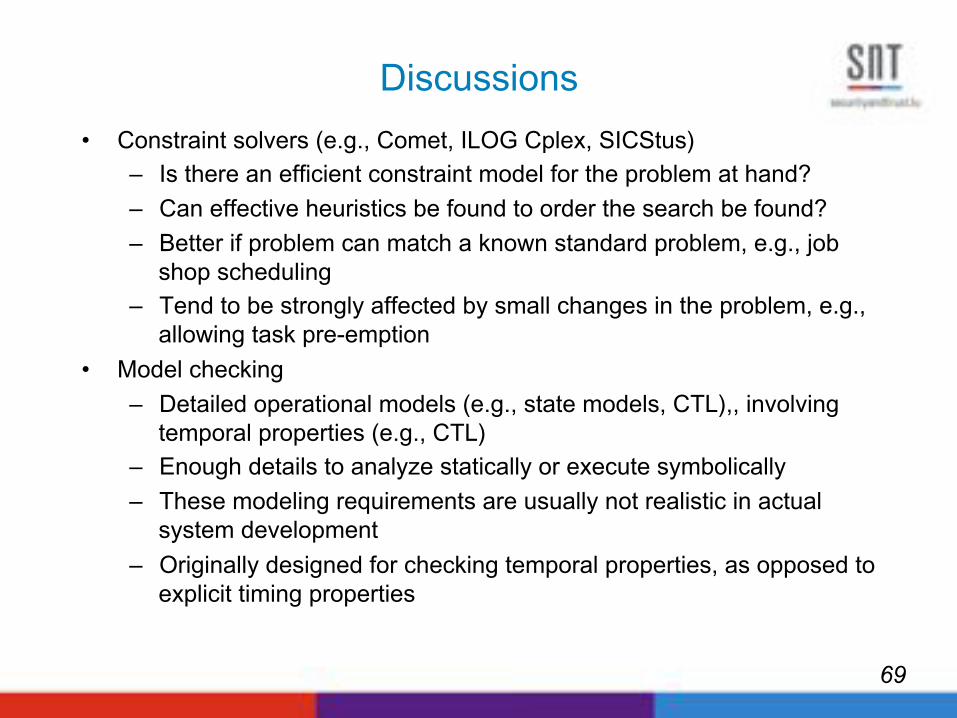
Discussions

•  Constraint solvers (e.g., Comet, ILOG Cplex, SICStus)

–  Is there an efficient constraint model for the problem at hand?

–  Can effective heuristics be found to order the search be found?

–  Better if problem can match a known standard problem, e.g., job shop scheduling

–  Tend to be strongly affected by small changes in the problem, e.g., allowing task pre-emption

•  Model checking

–  Detailed operational models (e.g., state models, CTL),, involving temporal properties (e.g., CTL)

–  Enough details to analyze statically or execute symbolically

–  These modeling requirements are usually not realistic in actual system development

–  Originally designed for checking temporal properties, as opposed to explicit timing properties

69

Discussions II

•  Metaheuristic search

–  Tends to be more versatile, tailorable to a new problem

–  Entail lower modeling requirements

–  Can provide responses at any time, without systematically and deterministically searching the same part of the space at every run

–  “best solution found within time constraints”, not a proof, no certainty

–  But in practice (complex) models are not fully correct, there is no certainty

70

Selected References

•  L. Briand, Y. Labiche, and M. Shousha, “Using genetic algorithms for early schedulability analysis and stress testing in real-time systems”, Genetic Programming and Evolvable Machines, vol. 7 no. 2, pp. 145-170, 2006

•  M. Shousha, L. Briand, and Y. Labiche, “UML/MARTE Model Analysis Method for Uncovering Scenarios Leading to Starvation and Deadlocks in Concurrent Systems”, IEEE Transactions on Software Engineering 38(2), 2012.

•  Z. Iqbal, A. Arcuri, L. Briand, “Empirical Investigation of Search Algorithms for Environment Model-Based Testing of Real-Time Embedded Software”, ACM ISSTA 2012

•  S. Nejati, S. Di Alesio, M. Sabetzadeh, L. Briand, “Modeling and Analysis of CPU Usage in Safety-Critical Embedded Systems to Support Stress Testing”, ACM/IEEE MODELS 2012

•  Shiva Nejati, Mehrdad Sabetzadeh, Davide Falessi, Lionel C. Briand, Thierry Coq, “A SysML-based approach to traceability management and design slicing in support of safety certification: Framework, tool support, and case studies”, Information & Software Technology 54(6): 569-590 (2012)

•  Lionel Briand et al., “Traceability and SysML Design Slices to Support Safety Inspections: A Controlled Experiment”, forthcoming in ACM Transactions on Software Engineering and Methodology, 2013

71

Selected References (cont.)

•  Rajwinder Kaur Panesar-Walawege, Mehrdad Sabetzadeh, Lionel C. Briand: Supporting the verification of compliance to safety standards via model-driven engineering: Approach, tool-support and empirical validation. Information & Software Technology 55(5): 836-864 (2013)

•  Razieh Behjati, Tao Yue, Lionel C. Briand, Bran Selic: SimPL: A product-line modeling methodology for families of integrated control systems. Information & Software Technology 55(3): 607-629 (2013)

•  Hadi Hemmati, Andrea Arcuri, Lionel C. Briand: Achieving scalable model-based testing through test case diversity. ACM Trans. Softw. Eng. Methodol. 22(1): 6 (2013)

•  Nina Elisabeth Holt, Richard Torkar, Lionel C. Briand, Kai Hansen: State-Based Testing: Industrial Evaluation of the Cost-Effectiveness of Round-Trip Path and Sneak-Path Strategies. ISSRE 2012: 321-330

•  Razieh Behjati, Tao Yue, Lionel C. Briand: A Modeling Approach to Support the Similarity-Based Reuse of Configuration Data. MoDELS 2012: 497-513

•  Shaukat Ali, Lionel C. Briand, Andrea Arcuri, Suneth Walawege: An Industrial Application of Robustness Testing Using Aspect-Oriented Modeling, UML/MARTE, and Search Algorithms. MoDELS 2011: 108-122

72