Scalability of Ad Hoc Routing Protocolscgi.di.uoa.gr/~istavrak/courses/05_PDT_Part4_Scal.pdf ·...

Ioannis Stavrakakis 2005 1

Scalability of Ad Hoc Routing Protocols

References:

C. Santivanez, R. Ramanathan, I. Stavrakakis, “Making Link-State Routing Scale for Ad Hoc Networks”, MobiHoc 2001, Oct. 4-5, 2001, Long Beach, CA, USA.

C. Santivanez, B. McDonald, I. Stavrakakis, R. Ramanathan, “ On the Scalability of Ad hoc Routing Protocols”, IEEE INFOCOM’02, N. York, USA.


Communication overhead Traditionally: overhead → control overhead

( = amount of bandwidth required to construct and maintain a route)

o In proactive approaches: number of packets exchanged in orderto maintain the node’s forwarding tables up-to-date

o In reactive approaches: bandwidth consumed by the routerequest/reply messages (global or local)

control overhead fails to include the impact of suboptimal routes

Suboptimal routes not only increase the end-to-end delay but also result in a greater bandwidth usage than required. As the network size increases keeping route optimality imposes an unacceptable cost.


Communication overhead

reactive protocols introduce suboptimal routes because: o they try to maintain the current source-destination path for as long as

it is valid, although it may no longer be optimal o local repair techniques try to reduce the overhead induced by the

protocol at the expense of longer, non optimal paths proactive protocols introduce suboptimal routes by: o limiting the scope of topology information dissemination (e.g. hierarchical routing) and/or o limiting the time between successive topology information updates

dissemination (topology updates are no longer instantaneously event-driven)


Communication overhead

revise the concept of overhead so that it includes the effect of suboptimalroutes The minimum traffic load of a network, is the minimum amount ofbandwidth required to forward packets over the shortest distance (in numberof hops) paths available, assuming all the nodes have instantaneous a priorifull topology information. routing protocol-independent metric assumes that all the nodes are provided a priori global information o possible in fixed networks o in mobile scenarios this is hardly possible

(even if static routes are provided it is unlikely that these remain optimal) motivates the definition of the total overhead of a routing protocol


Minimum traffic load – Total overhead

Total amount of bandwidth = minimum traffic load + total overhead

routing protocol

dependent

routing protocol

independent

routing protocol

dependent The total overhead induced by a routing protocol is the difference between the total amount of bandwidth actually consumed by the network running such routing protocol minus the minimum traffic load that would have been required should the nodes had a priori full topology information.


Minimum traffic load – Total overheadThe total overhead : provides an unbiased metric for performance comparison that

reflects bandwidth consumption may not fully characterize all the performance aspects relevant to

specific applications, but o bandwidth is likely to remain a limiting factor in terms of

scalability o bandwidth is proportional to factors including energy

consumption, memory and processing requirements The different sources of overhead may be expressed in terms of o Reactive routing overhead o Proactive routing overhead o suboptimal routing overhead


Proactive, Reactive & Suboptimal overheadThe reactive overhead of a protocol is the amount of bandwidthconsumed by the specific protocol to build paths from a source to adestination, after a traffic flow to that destination has been generated at the source.

In static networks is a function of the rate of generation of newflows.

In dynamic (mobile) networks is a function of both the traffic andthe rate topology change. (paths are (re)built not only due to new flows but also due to link failures in analready active path)


Proactive, Reactive & Suboptimal overheadThe proactive overhead of a protocol is the amount of bandwidthconsumed by the protocol in order to propagate route information before it is needed.

The suboptimal routing overhead of a protocol is the difference betweenthe bandwidth consumed when transmitting data from all the sources totheir destinations using the routes determined by the specific protocol, andthe bandwidth that would have been consumed should the data havefollowed the shortest available path(s).

Example: a source that is 3 hops away from its destination

a protocol chooses to deliver one packet following a k ( 3k > ) hop path (for example, due to out-of-date information) ⇒ ( 3)k packet_length− ∗ bits will be added to the suboptimal RO


Achievable Regions & Operating points The 3 different overhead sources are locked in a 3-way trade-off

in an already efficient algorithm, the reduction of one of them willmost likely cause the increase of one of the others

For example, reducing the ‘zone’ size in ZRP: • will reduce ZRP’s proactive overhead, but • will increase ZRP’s reactive overhead

achievable region of overhead: The three dimensional region formed by all the values of proactive,reactive, and suboptimal routing overheads that can be induced by anyprotocol under the same scenario (traffic, mobility, etc.)


Achievable Regions & Operating points Figure: 2-dimensional transformation of the ‘achievable region’ • horizontal axis: proactive overhead induced by a protocol • vertical axis: reactive + suboptimal routing overheads Proactive cost (per node)

AchievableRegion

Ext

ra b

andw

idth

usa

ge p

er n

ode

(sub

-opt

imal

rout

es, r

oute

requ

est,e

tc.)


Achievable Regions & Operating pointsthe achievable region

is convex o consider the points 1P and 2P achieved by protocols 1P and 2P o any point 1 2(1 )P Pλ λ+ − can be achieved by engaging protocol

3P that behaves as protocol 1P a fraction λ of a (long) time as protocol 2P the remaining of the time

is lower-bounded by the curve of overhead points achieved by the‘efficient’ protocols (‘efficient’ protocols: minimize some source of overhead given a conditionimposed on the others)


Achievable Regions & Operating points

the best protocol

(in terms of overhead)

→

minimizes total overhead

⇔

achieves point Opt

point Opt : point tangent to the curve x y constant+ =

P → best pure proactive approach (reactive overhead = 0) given that optimal routes are required (suboptimal overhead= 0) P moves to the right as mobility increases R → best protocol that does not use any proactive information R moves upward as traffic increases or diversifies


Effect of increasing the network size

the boundary region is pulled up the region displacement

is not uniform

P

R


Effect of increasing the network size

points P and R increase proportionally to 2( )NΘ

Pure proactive protocols (SLS) [Pure reactive algorithms (DSR without the route cache option)] generate a control message [a route request (RREQ) message] each time a link changes (worst case) [a new session is initiated]

Each control message [RREQ message] is retransmitted by each node

The generation rate of control messages [RREQ messages]increases linearly with network size ( N )

The number of message retransmissions increases linearly with N

⇒ The total overhead increases as rapidly as 2N


Effect of increasing the network size As size increases, the best operating point is far from the extreme points P and R and in the region where the proactive, reactive, and suboptimal routing overheads are balanced.

Protocols inducing ‘intermediatepoints’:

• Hierarchical link state (HierLS): 1 5N . • ZRP: 1 66N .

R

P


Network’s scalability (Qualitatively)

Scalability is the ability of a network to support the increase of its limiting parameters. Limiting parameters of a network are those parameterwhose increase causes the network performance to degrade. For example:

mobility rate

traffic rate

network size

network density


Network’s scalability (Quantitatively)Let 1 2( )Tr …λ λ, , be the minimum traffic load experienced by a network under parameters 1 2 …λ λ, , . Then, the network scalability factor of such a network, with respect to a parameter iλ (

iλΨ ) is: def

1 2log ( )limlogi

i i

Tr …λ λ

λ λλ→∞

, ,Ψ =

relates the increase in network load to the different network parameters may be used to compare the scalability properties of differentnetworks (wireline, mobile ad hoc, etc.)

For the class of mobile ad hoc networks defined by assumptions a.1-a.8 the minimum traffic load ( )lc tTr Nλ λ, , = 1 5( )t Nλ .Θ

⇒ 0lcλΨ = , 1

tλΨ = , and 1 5NΨ = .


Network’s scalability (Quantitatively) to assess whether a network is scalable w.r.t. to iλ

the network rate dependency on iλ must be considered The network rate networkR of a network is the maximum number ofbits that can be simultaneously transmitted in a unit of time. For the network rate ( networkR ) computation all successful link layertransmissions must be counted, regardless of whether the link layerrecipient is the final network- layer destination or not.


Network’s scalability (Quantitatively)

A network is said to be scalable with respect to the parameter iλif and only if, as the parameter iλ increases, the network’s minimum traffic load does not increase faster than the network rate ( networkR ) can support. That is, if and only if:

1 2log ( )limlogi

i

network

i

R …λ λ

λ λλ→∞

, ,Ψ ≤



For example, class of networks under study (assumptions a.1-a.8) (resulting from applying power control techniques) 1 5NΨ = .

to be regarded as scalable with respect to network size 1NΨ ≤ (It has been shown [Gupta, Kumar 2000] that in mobile ad hoc networksΘ(Ν) successful transmissions can be scheduled simultaneously. I.E., thenetwork rate is Θ(Ν) )

⇒ networks under study are not scalable w.r.t. to network size



Note: It has been shown in [Groossglauser&TSE, Infocom 2001] that if the network applications can support infinitely long delays and themobility pattern is completely random, then the average path lengthmay be reduced to 2 ( )Θ(1 ) regardless of network size and, as aconsequence, that network scalability factor with respect to network size ΝΨ is equal to 1. Thus, those ad hoc networks (random mobility and capable of accepting infinitely long delays) are the only class of ad hoc networks that are scalable with respect to network size. Thiswork does not consider that class of networks since they have nopractical relevance.


Network’s scalability (Quantitatively) Wireline networks: if fully connected may have 1NΨ =

⇒ potentially scalable w.r.t. network size (in the bandwidth sense) (However, this scalability requires the nodes’ degree to grow without bound, which may be prohibitely expensive)

Similarly, the network rate does not increase with mobility or traffic load

(Gupta – Gunar result: Θ(N)) ⇒ a network will be scalable w.r.t. mobility ⇔ 0

lcλΨ = w.r.t. traffic ⇔ 0

tλΨ = ⇒ the networks under study

o are scalable w.r.t. mobility o but are not scalable w.r.t. traffic



Similar conclusions for scalability w.r.t. additional parameters For example, as transmission range increases the spatial reuse decreases

(assuming a infinite size network with regular density) network rate decreases as rapidly as 2l

⇒ Ψl should be lower than 2− for the network to be scalable ⇒ ad hoc networks are not scalable w.r.t. transmission range (the minimum traffic load decreases only linearly w.r.t. l => 1Ψ = −l ) ⇒ focus on networks with power control (the transmission range changes so that the network degree is kept bounded)


Routing Protocol’s scalability (Qualitatively) mobile ad hoc networks are not scalable with respect to size

How about routing protocol scalability?

Routing protocol’s scalability is the ability of a routing protocol tosupport the continuous increase of the network parameters withoutdegrading network performance. the network’s own scalabilty properties provide the reference levelas to what to expect of a routing protocol

If the overhead induced by a routing protocol grows slower than the minimum traffic load then the routing protocol is notdegrading network performance (determined by the minimum traffic load), even if the overhead happens to grow faster than the network rate.


Routing Protocol’s scalability (Quantitatively) Let 1 2( )ovX …λ λ, , be the total overhead induced by routing protocol X , dependent on parameters 1 2 …λ λ, , (e.g. network size, mobility rate, datageneration rate, etc.). Then, the Protocol X’s routing protocol scalability factorwith respect to a parameter iλ (

i

Xλρ ) is defined to be :

def1 2log ( )lim

logii

X ov

i

X …λ λ

λ λρλ→∞

, ,=

provides a basis for comparison among different routing protocols


Routing Protocol’s scalability (Quantitatively)(to assess whether a routing protocol is scalable the following definition is used)

A routing protocol X is said to be scalable with respect to the parameter iλif and only if, as the parameter iλ increases, the total overhead induced by such protocol ( ovX ) does not increase faster than the network’s minimum traffic load. That is, if and only if:

i i

Xλ λρ ≤ Ψ

for the class of network under study, a routing protocol X is: o scalable w.r.t. network size ⇔ 1 5X

Nρ ≤ .

o scalable w.r.t. mobility rate ⇔ 0lc

Xλρ ≤

o scalable w.r.t. traffic ⇔ 1t

Xλρ ≤


Scalability dimensions network size is a key parameter, but not the only one

(mobility, network density, network diameter, traffic diversity, energy etc.) Examples :

diameter ↑ => latency for control ↑ => inconsistent routes, instability↑ density↑ spatial reuse ↓ => capacity ↓

dimension

layer

Size Mobility Density Diameter

Transport × × Network ⊗ ⊗ × ×

Link/MAC × × Physical ×

Key scalability dimensions and their effect on the lower four layers (in addition to traffic)


Scalability dimensions size, density, diameter, and transmission range are related

given size & density, different transmission power levels ( ↓ ) result in different (node degree ( ↓ ) , network diameter ( ↑ ))

in order to increase the overall network performance, the average node degree must remain bounded (provided (bi-)connectivity)

density dimension can be addressed by means of effective topology (transmission power) control algorithms

Focus on: network size, mobility & traffic load assuming topology control (diameter and size are mutually dependent, density is not a limiting factor)


Network model: NotationsN : number of nodes in the network

d : average in-degree

L : average path length over all source destination pairs

lcλ : expected number of link status changes that a node detects (/sec)

tλ : average traffic rate that a node generates in a second (in bps)

sλ : average number of new sessions generated by a node in a second


Standard asymptotic notations

( ) ( ( ))f n g n= Ω if ∃ 1c , 1n : 1 ( ) ( )c g n f n≤ , 1n n∀ ≥

( ) ( ( ))f n O g n= if ∃ 2c , 2n : 2( ) ( )f n c g n≤ , 2n n∀ ≥

( ) ( ( ))f n g n= Θ if ∃ 1 2c c, , and 0n : 1 2( ) ( ) ( )c g n f n c g n≤ ≤ , 0n n∀ ≥

1 2c c, constants


Assumptions o a.1 As the network size increases, the average in-degree d remains

constant.

imposing a fixed degree in a network is:

o desirable (density increase jeopardizes the achievable throughput)

o achievable (through effective power control mechanisms)

a topology control algorithm should:

o make the density as small as possible

o without compromising (bi)connectivity


Assumptionsa.2 : Let A be the area covered by the N nodes of the network, and N Aσ = / be the network average density. Then, the expected (average) number of nodes inside an area 1A is approximately 1Aσ ∗ .

on large scales uniformity is expected to increase (for example, it is expected that half the area contains approx. ½ of the nodes)

focus on expected (mean) behavior (for a specific network topology this assumption may not hold)

geographical reasoning may not define one hop connectivity (where multipath fading, obstacles, etc. are more important)

however, it strongly influences connectivity (as observed according to larger scales)


Assumptions

a.2 Let A be the area covered by the N nodes of the network, and N Aσ = / be the network average density. Then, the expected (average)

number of nodes inside an area 1A is approximately 1Aσ ∗ .

One can talk about the `geographical' and `topological' regions.

In the `geographical' (large-scale) region, geographical-based reasoning shapes routing decisions.

In the `topological' region, it is the actual link connectivity (topology) that drives the routing decisions, and geographical insights are less useful.


Assumptions a.3 : The number of nodes that are at distance of k or less hops away from a source node increases (on average) as

2( )d kΘ ∗ . The number of nodes exactly at k hops away increases as ( )d kΘ ∗ .

a.4 : The maximum and average path length (in hops) among nodes in a connected subset of n nodes both increaseas ( )nΘ . In particular, the maximum path length acrossthe whole network and the average path length across thenetwork ( L ) increases as ( )NΘ .

a.3 and a.4 are based on a.2


Assumptions

a.3 , a.4

a.3 and a.4 are based on a.2 example: a circular area centered at node S of radius R with n nodes If R → R2 o covered area, number of nodes inside the area → 4x o distance (in meters) from S to the farthest nodes → 2x o distance (in hops) from S to the farthest nodes → 2x (assuming that the transmission range of the nodes does not change) o `boundary' area (where the nodes farthest away from S are) → 2x

SR

2R


Assumptionsa.5 : The traffic that a node generates in a second ( tλ ), is independent of the network size N (number of possible destinations). As the network size increases, the total amount of data transmitted/received by a single node will remain constant but the number of destinations will increase(the destinations diversity will increase).

a.6 : For a given source node, all possible destinations ( 1N − nodes) are equiprobable and – as a consequence of a.5 – the traffic from one node to every destination decreases as (1 )NΘ / .

a.5 & a.6 : As the network size increases the total amount of traffic generated by a single user typically diversifies rather than increases.

a.5 & a.6 are first order approximations motivated by observed behaviorwith existing networks (human users)

some other networks may violate these assumptions


Assumptionsa.5 & a6

Examples: low-cost long distance service: a user speaks with more friends

(wherever they are), but does not increase the total time the user has tospare for personal phone calls

increase in size and content of the Internet: a user may find more web pages (destination set diversifies) but he/she will limit the total time (andtraffic) spent on the Internet

Sensor networks may violate these assumptions o each node may broadcast its information to all other nodes

( tλ increases as )(ΝΘ )

o or, may transmit to a central node (causing the destination set to consist of only 1 node, violating a.6)


Assumptions a.6

Traffic assumption largely determines the effect of suboptimalrouting on performance.

o limited to the locality of the source ⇒ hierarchical routing, ZRP, andNSLS will benefit

o small set of destinations will favor algorithms such as DSR

o uniform traffic tends to favor proactive approaches such as link state

Equally distributed traffic (a.6) tends to pose the most demandingrequirements on a routing protocol.

A protocol that is scalable (with respect to traffic) under a.6, willalso be scalable under any other traffic pattern.


Assumptionsa.7 : Link status changes are due to mobility. lcλ is directly proportional to the relative node speed.

assumption: short-lived link degradation will not trigger updates short-term variations in link quality can be offset by link control mechanisms for example:

• by requiring a high fading margin before declaring a link up

• by waiting for several seconds before declaring a link down

wireless channel is quite unpredictable and long-lived link degradation is possible without mobility


Assumptionsa.8 : Mobility models : time scaling.

Let 1 0 ( )f x y/ , be the probability distribution function of a node position attime 1 second, given that the node was at the origin (0 0), at time 0 . Then, the probability distribution function of a node position at time tgiven that the node was at the position

0 0( )t tx y, at time 0t is given by

0 020 0 0 0 00

11 0( )

( ) ( )t tx x y yt t t t t t t tt t

f x y x y f − −/ / − −−

, , , = , .

motivated by mobility models where the velocity of a mobile over timeis highly correlated

for example, this is the case if the unknown speed and direction are constant does not hold for a random walk model

induces smaller node displacements over time ( )( tΘ , t : elapsed time

focus on the most demanding scenario (larger displacements)


Routing protocol scalability conditions for the networks subject to assumptions a.1-1.8

For the class of mobile ad hoc networks defined by assumptions a.1-a.8 the minimum traffic load ( )lc tTr Nλ λ, , = 1 5( )t Nλ .Θ and thus :

0

lcλΨ = , 1tλΨ = , and 1 5NΨ = .

Consequently, for the class of network under study, a routing protocol X is: o scalable w.r.t. mobility rate ⇔ 0

lc

Xλρ ≤

o scalable w.r.t. traffic ⇔ 1t

Xλρ ≤

o scalable w.r.t. network size ⇔ 1 5XNρ ≤ .


Plain Flooding (PF) PF reactive RO = PF proactive RO = 0

PF suboptimal RO / sec = 2 1 5 2( ( )) ( )t tN N Nλ λ.Θ − = Θ

t Nλ data packets are generated / sec 1N − transmissions / packet

(is (re)transmitted by every node, except the destination) optimal value (on average) = L , ( )L N= Θ (a.4)

(up to L hops broadcast needed, the rest is OH) ⇒ additional bandwidth required = ( 1 ) tdata N L Nλ− − bps

PF total RO /sec = 2( )t NλΘ ∗

⇒ 0lc

PFλρ = , 1

t

PFλρ = , 2PF

Nρ =


Standard Link State (SLS) SLS reactive RO = SLS suboptimal RO = 0

SLS proactive RO / sec = 2lclsu Nλ bps = 2( )lc NλΘ

lsu := size of the LSU (Link State Update) packet

lcNλ LSUs are generated /sec (in average) (each node generates an LSU at a rate of lcλ / sec)

overhead of lsu N bits / LSU (each LSU is transmitted at least N times (once/node))

SLS total RO / sec = 2

lclsu Nλ bps = 2( )lc NλΘ ⇒ 1

lc

SLSλρ = , 0

t

SLSλρ = , 2SLS

Nρ = .


Dynamic Source Routing (DSR) no proactive information is exchanged

A node (source) reaches a destination by flooding the network

with a route request (RREQ) message. When an RREQ message reaches the destination (or a node with a

cached route towards the destination) a route reply message is sent back to the source, including the newly found route

The source attaches the new route to the header of all subsequentpackets to that destination, and any intermediate node along the routeuses this attached information to determine the next hop in the route.

focus on DSR without the route cache option (DSR-noRC)


DSR without Route Cache (DSR-noRC)DSR-noRC reactive RO

RREQ (route request) messages are generated by: new session requests (at a rate sλ per second per node) failures in links that are part of a path currently in use

only new requests are considered ⇒ a lower bound is obtained

s Nλ RREQ messages are generated / sec (new session requests) overhead of ( 1)size_of_RREQ N − bits / RREQ message

(each RREQ message is flooded ⇒ 1N − retransmissions)

⇒ DSR-noRC reactive RO / sec = 2( )s NλΩ upper bound 2(( ) )s lcO Nλ λ+

(assumption: each link failure has the same effect as a new sessionrequest (local repair fails))


DSR without Route Cache (DSR-noRC)DSR-noRC suboptimal RO

• only the extra bandwidth required for appending the source-route in each data packet is considered ⇒ a lower bound is obtained

• number of bits appended in each packet ~ length iL of path iopt

i iL L≥ (optimal path length), optiL instead of iL ⇒ lower bound

extra bits for a packet delivered using a path i : 22(log )( )opt

iN L

o at least optiL retransmissions of at least opt

iL 2log N bits o 2log N is the minimum length of a node address


DSR without Route Cache (DSR-noRC) extra bits for a packet delivered using a path i : 2

2(log )( )optiN L

extra bits / packet over all paths (average):

2 2 22 2 2(log )( ) ) (log ) (log )opt opt

i iE N L N E L N L≥ = bits t Nλ packets are transmitted / sec

⇒ suboptimal RO at least 2

2(log )t N N Lλ bps, ( )L N= Θ (a.4) ⇒ DSR-noRC suboptimal RO / sec = 2

2( log )t N NλΩ bps


DSR without Route Cache (DSR-noRC)DSR-noRC reactive RO / sec = 2( )s NλΩ = 2(( ) )s lcO Nλ λ+ DSR-noRC suboptimal RO / sec = 2

2( log )t N NλΩ bps

DSR-noRC total overhead / sec = 2 22( log )s tN N Nλ λΩ +

1t

DSR noRCλρ − = , 0 1

lc

DSR noRCλρ −< <= , 2DSR noRC

Nρ − >


Hierarchical Link State (HierLS)The network organized in m level clusters, each of equal size k( mN k= ), k is predefined while m increases with N . Location Management (LM) service choices:

LM1 Pure proactive.

LM2 Local paging.

LM3 Global paging.


HierLS-LM1 Total Overhead HierLS-LM1 proactive RO = 1 5( )lcs N Nλ.Ω + HierLS-LM1 suboptimal RO / sec = 1 5( )tN

δλ . +Θ ⇒ HierLS-LM1 total overhead / sec

= 1 5 1 5( )lc ts N N N δλ λ. . +Ω ∗ + ∗ + ⇒ 1 1

t

HierLS LMλρ − = , 1 1

lc

HierLS LMλρ − = , and 1 1 5 1 5HierLS LM

Nρ δ− = . + > . (HierLS is almost scalable w.r.t. network size)


HierLS-LM2 Total Overhead HierLS-LM2 suboptimal RO / sec =

= HierLS-LM1 suboptimal RO / sec = 1 5( )t Nδλ . +Θ

HierLS-LM2 proactive RO = = HierLS-LM1 proactive RO = 1 5( )lcs N Nλ.Ω +

HierLS-LM2 reactive RO = ( )tO Nλ ⇒ HierLS-LM2 total overhead = 1 5 1 5( )lc ts N N N δλ λ. . +Ω + + same asymptotic scalability factors as HierLS-LM1


HierLS-LM3 Total Overhead HierLS-LM3 suboptimal RO / sec =

= HierLS-LM1 suboptimal RO / sec = 1 5( )t Nδλ . +Θ

HierLS-LM3 proactive RO = ( log )s N NΘ lc Nλ+

HierLS-LM3 reactive RO = 1 5( )tO N δλ . + ⇒ HierLS-LM3 total overhead = 1 5( log )lc ts N N N N δλ λ . +Ω + + same asymptotic scalability factors as HierLS-LM1


Zone Routing Protocol (ZRP) lower bound for for ZRP’ total overhead (can be prooved)

ovZRP = 2( )k lc s kn N N nλ λΩ + /

where: kn = average number of nodes inside node’s ‘zone’

o proactive overhead: ( )k lcn NλΩ

o reactive overhead: 2( )s kN nλΩ /

(For the sub-optimal routing overhead an upper bound can be proved that shows that it is (asymptotically) dominated by the reactive overhead)

Minimizing this lower bound by properly choosing the value kn

23(( ) )s

lc

Nkn λ

λ= Θ ⇒ 51 2

3 3 3( )lc s Nλ λΩ


Flat Routing flat'' ≠ hierarchical

each node and link in the topology table is an actual node or link

(no topology abstraction, no ``boundaries'', no hierarchical addressing)

the topology table may grow large as the network size increases

usually require much more memory and processing power (however, the main challenge is the excessive bandwidth)

require careful design (else may result in much more bandwidth consumption than hierarchical) Techniques for bandwidth consumption reduction: (in isolation or in combination) o efficient flooding o limited generation o limited dissemination


Efficient Flooding classical flooding is a very inefficient

(each node receives the same packet several times) Efficient flooding:

o reduce the number of times a message is retransmitted o each recipient should receive each message at least once Example (mechanism):

o find a tree that covers all the nodes o propagate the message across all the nodes in the tree (every node in the tree transmits the message only once) Examples (protocols): o Optimized Link State Routing (OLSR) o Topology Broadcast based on Reverse Path Flooding (TBRPF) o Core Extraction Distributed Ad-Hoc Routing (CEDAR)


Limited Generation

limit the amount of control information

Examples update generation at times which are multiples of a base period et

(effective for high mobility)

o Global State Routing (GSR) o Discretized Link State (DLS)

updates only for changes that affect another node's best route o Source-Tree Adaptive Routing (STAR)

operating on connected subgraphs o OLSR


Limited Dissemination reduced depth of propagation of routing updates

o most updates sent to a subset of nodes (not the entire network) o the subset may change over time

promise for scalability improvement o especially for networks with a large diameter o challenge: not to overly compromise route optimally

Examples

ZRP, NSLS limit the update propagation to k-neighbors only Fisheye State Routing

o Network = “in-scope” + “out-of-scope” subsets o out-of-scope nodes are “informed” with a smaller frequency

family of Fuzzy Sighted Link State (FSLS) algorithms o LSU generation: at multiples of a base time et o a LSU (in general) travels TTL hops o TTL depends on the current time


FSLS AlgorithmsObservation: Nodes that are far away do not need to have complete topological information in order to make a good next hop decision, thuspropagating every link status change over the network may not benecessary.

(in hop-by-hop routing, changes experienced by nodes far away tend to have little impact in a node’s ‘local’ next hop decision)

pure proactive protocol (as SLS) do not scale well with size

(the induced overhead increases as rapidly as 2N )

a reduction of the proactive overhead may be achieved: o in space

(by limiting which nodes the link state update is transmitted to) o in time

(by limiting the time between successive link status updates)

balance is necessary (a reduction on proactive RO will induce an increase in suboptimal RO)


FSLS AlgorithmsFamily of Fuzzy Sighted Link State (FSLS)

the frequency of Link State Updates (LSUs) propagated to distantnodes is reduced

a node transmits a Link State Update (LSU) o only at particular time instants

(potentially several link changes are ‘collected’)

o the Time To Live (TTL) field of the LSU is set to a value (specifies how far the LSU is propagated)

that is a function of the current time


FSLS AlgorithmsUnder a FSLS protocol

& after one global LSU transmission (TTL =∞) (for example, during initialization)

a node: wakes up every 12i

et− ∗ ( 1 2 3i = , , ,... ) seconds

and transmits a LSU with TTL set to is (if there has been a link status change in the last 12i

et− ∗ seconds)

i.e.: ‘wakes up’ every et seconds and sends a LSU with TTL set to 1s (if there has been a link status change in the last et seconds)

wakes up every 2 et∗ seconds and transmits a LSU with TTL set to 2s (if there has been a link status change in the last 2 et∗ seconds) …


FSLS Algorithms

Strictly speaking, the node will consider link changes since the lasttime a LSU with TTL greater or equal to is was considered (not necessarily transmitted).

If the value of is is greater than the distance from this node to any other node in the network, the TTL field of the LSU is set to infinity(global LSU), and all the counters and timers are reset.

As a soft state protection on low mobility environments, a periodictimer may be set to ensure that a global LSU is transmitted at least each

bt seconds.


FSLS AlgorithmsExample of FSLS’s LSU generation process

(mobility is high ⇒ LSUs are always generated every et seconds)

the sequence 1 2s s …, , is non-decreasing


FSLS AlgorithmsFor example, time 4 et is a multiple of et (associated with 1s ), 2 et (associated with 2s ) and4 et (associated with 3s )

if there has been a link status change in the past et or 2 et seconds, then there has been a link change in the past 4 et seconds ⇒ if we have to set the TTL field to at least 1s (or 2s ) we also have to increase it to 3s

if there has not been a link status change in the past 4 et seconds, then there has not been a link change in the past et or 2 et seconds ⇒ if we do not send a LSU with TTL = 3s , we do not send a LSU at all

At times 4 ek t∗ ∗ ( k odd) the link state change activity during the past 4 etseconds is checked and, if there is any, then an LSU with TTL set to 3s is sent. (In the highly mobile scenario assumed on the figure, a LSU with TTL equal to

3s is sent at times 4 et and12 et .)


FSLS Algorithms nodes that are is hops away from a tagged node will learn about a

link status change at most after 12 iet

− seconds (‘refresh’ time) ( )T r determines the

latency in the link state information

Different approaches may be implemented by considering different is sequences. o Discretized Link State

(DLS) o Near Sighted Link State

(NSLS) Maxi mu m refresh time as a function of distance fro m link event.


FSLS Algorithms: Discretized Link State (DLS)

DLS is obtained by setting is = ∞ for all i

is similar to the Standard Link State (SLS)

difference: under DLS a LSU is not sent immediately after a link status change (only when the current et interval is completed) ⇒ several link status changes may be collected in one LSU (modification of SLS that attempts to scale better w.r.t. mobility)


FSLS Algorithms: Discretized Link State (DLS) Under high mobility

some similarities with Global State Routing (GSR)

In GSR, a node exchanges its version of the network topology tablewith its one-hop neighbors each floodt seconds. (limits the frequency of link state updates to be no greater that 1

floodt )

Under high mobility (LSUs are sent every et seconds) DLS induces

the same proactive overhead as GSR (by setting e floodt t= ) (they both require control packets transmission of the equivalent of N times the average topology table size (in bits) each et ( floodt ) seconds)


FSLS Algorithms: Near Sighted Link State (NSLS)

NSLS is obtained by

setting o is k= for i p< o ps = ∞ ( p integer)

a node receives information only from nodes inside its sight area (that are less than ‘k’ hops away )


FSLS Algorithms: NSLSProblem

Suppose that initially a node knows routes to every destination.

as time evolves nodes move, links go down o the node learns that the previous routes will fail o the node does not learn of new available routes (out-of-sight information is not being updated)

common to every algorithm in the FSLS family (NSLS represents its worst case scenario) Solution

the node uses the ‘memory’ of past links o sends packets in the direction it ‘saw’ the destination for the last time o if the packet gets to a node that is on the ‘sight’ of the destination,

this node can forward the packet to the destination.


FSLS Algorithms: NSLSNSLS has similarities with: the proactive part of the Zone Routing Protocol (ZRP)

(without the reactive route search) the Distance Routing Effect Algorithm for Mobility (DREAM)

difference: NSLS limits the LSU propagation based on the number of hops traversed DREAM limits the position update message’s propagation based on the geographical distance to the source


FSLS Algorithms: NSLSNSLS has similarities with Fisheye State Routing (FSR) : FSR uses the same topology dissemination mechanism as GSR, but itdoes not transmit the whole topology information each floodt seconds. (only a short version including only the closest nodes entries is transmitted) A second, larger timer ( larget ) is used for out-of-scope nodes Setting e floodt t= and b larget t= , & k : all the nodes in-scope are k or less hops away ⇒ NSLS induces the same control overhead as FSR


FSLS Algorithms: NSLS the latency in updating link state information is greater in FSR

NSLS: ( ) eT r t= for r k≤ , and ( ) bT r t= for r k> FSR: ( ) eT r t r= ∗ for r k≤ , and ( ) ( )e bT r k t r k t= ∗ + − ∗ (In FSR, a LSU waits at most et to be propagated one more hop away, if it isin scope ( r k≤ ) and waits bt seconds when it is ‘out-of-scope’ (i.e. r k> )).

NSLS FSR


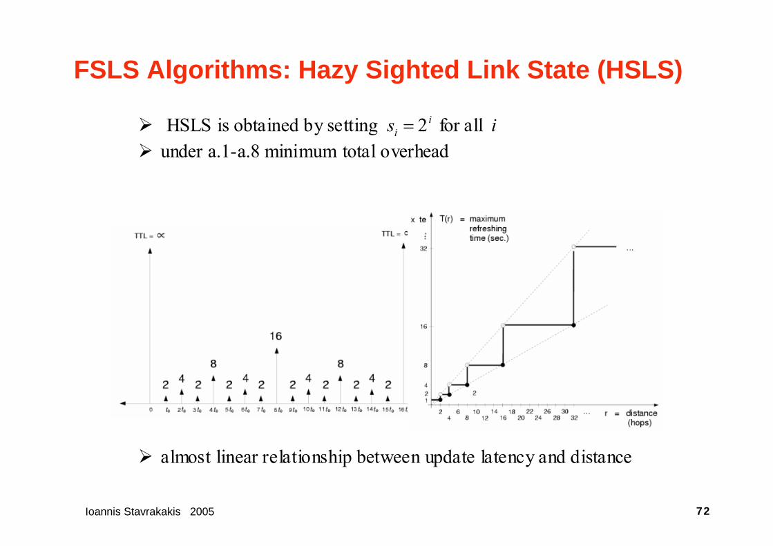
FSLS Algorithms: Hazy Sighted Link State (HSLS)

HSLS is obtained by setting 2 iis = for all i

under a.1-a.8 minimum total overhead

almost linear relationship between update latency and distance


FSLS Algorithms: Hazy Sighted Link State (HSLS)

latency versus distance curve: optimal performance when linear (optimal balance between proactive and sub-optimal routing overhead)

it turns out that angular uncertainty is roughly constant (independent of the distance) o hop-by-hop routing is based on the next hop decision o Prob. of wrong decision depends mainly in the angular uncertainty o If constant ⇒ Prob. of bad next hop decision is constant

Intuitively:

If faster than linear, too many mistakes when forwarding packets to nodes far away

If slower than linear, fewer mistakes, but the proactive overhead increases


Asymptotic Results

Protocol Proactive Reactive Suboptimal PF – – 2( )t NλΘ

SLS 2( )lcNλΘ – – DSR-noRC – 2( )sNλΩ 2

2( log )t N NλΩ 2(( ) )s lcO Nλ λ+

HierLS 1 5( )lcsN Nλ.Ω + – 1 5( )tNδλ . +Θ

ZRP ( )k lcn NλΘ 2( )s kN nλΩ / 2( )t kO N nλ / HSLS 1 5( )eN t.Θ / – 4 1 5(( 1) )lc et K

te Nλ λ .Θ −


Asymptotic expressions

Best possible total overhead bounds for mobile ad hoc networks protocols

Protocol Total overhead (best) Cases PF 2( )t NλΘ Always

SLS 2( )lcNλΘ Always DSR-noRC 2 2

2( log )s tN N Nλ λΩ + Always

HierLS 1 5 1 5( )lc tsN N N δλ λ. . +Ω + + LM1 ZRP 2( )lc NλΩ if ( )lc sO Nλ λ= /

51 23 3 3( )lc s Nλ λΩ if ( ) and ( )lc s lc sN O Nλ λ λ λ= Ω / =

2( )sNλΩ if ( )lc sNλ λ= Ω HSLS 1 5( )lc t Nλ λ .Θ if ( )lc tOλ λ=

1 5( )lc Nλ .Θ if ( )lc tλ λ= Ω


Observing the asymptotic expressionsw.r.t network size

HierLS and HSLS scale better

flooding to the entire network (link state, route request, or data) ⇒ routing protocol scalability factor w. r.t. network size = 2

splitting the information dissemination at two different levels (like in 2-level hierarchical routing, NSLS, ZRP, and DREAM) ⇒ routing protocol scalability factor w.r.t. network size = 1.66

allowing the number of levels grow as the network size increases (as done explicitly by m-level HierLS and implicitly by HSLS) ⇒ routing protocol scalability factor w.r.t. network size = 1.5 (seems to be the limit for routing protocols for networks defined by a.1-a.8)


Observing the asymptotic expressions

w.r.t traffic intensity SLS, and ZRP scale better (total overhead is independent of tλ )

HSLS follows (scales as ( )tλΘ ) PF, DSR, and HierLS are the last (total RO ~ traffic)

ZRP adapts its zone size (→ pure proactive) HSLS increases its LSU generation rate

(reducing update latency and improving the quality of the routes) Conclusion: as traffic load increases 1. the quality of the routes becomes more and more important 2. more bandwidth should be allocated for routing (to improve quality) 2. contradicts the widely held belief that as traffic load is increased, less bandwidth should be allocated to control traffic and let more bandwidth available for user data


Observing the asymptotic expressionsw.r.t. the rate of topological change

PF total RO is independent of the rate of topological change if the rate of topological change increases too rapidly may be preferred (especially, if size and traffic are small)

ZRP and DSR are next their lower bounds are independent of the rate of topological changes (their behavior should depend somewhat of the rate of topological change)

SLS, HierLS, and HSLS their total overhead increases linearly w.r.t. the rate of topological change


Observing the asymptotic expressionsIt is interesting to note that:

if mobility OR traffic increase ZRP achieves almost the best performance

if mobility AND traffic increase at the same rate ( ( )lcλ λ= Θ and ( )tλ λ= Θ (for some parameter λ )) ZRP’s scalability w.r.t λ same as HSLS’s and HierLS’s ZRP: 1 66( )Nλ .Ω , HSLS: 1 5( )Nλ .Θ , HierLS’s: 1 5( )N δλ . +Θ

HSLS scales better with traffic intensities than HierLS (the only other protocol that scales well with size)

intuitive explanation: o HierLS never attempts to find optimal routes (even under slowly changing conditions) o HSLS may obtain full topology information =>optimal routes (if the rate of topological changes is small w.r.t. 1/ et )


Comparing HierLS and HSLS both scale well w.r.t. network size

(both induce a multi-level information dissemination technique)

HSLS's routes' quality does not degrade with network size (angular displacement uncertainty depends mainly on the nodes speed and et )

HierLS's routes's quality suffers small degradation each time the number of hierarchical levels is increased

HSLS is able to improve the quality of its routes as a response to an increase in traffic load

HierLS's route quality dependents on the number of hierarchical levels (which depend on the cluster size (independent of the traffic load)) ⇒ HierLS can not react to an increase in traffic load


Comparing HierLS and HSLS theoretical analysis focuses on asymptotically large networks, heavy

traffic load, and saturation conditions

What about the constants involved in the asymptotic expressions? (and the effect of other factors (MAC, latency on detecting failures, etc.)) ⇒ Simulations: medium size network with moderate loads

Simulator: OPNET Topology: 400 randomly located nodes on a square (320square miles) Mobility: Each node chooses a random direction (among 4) and

moves at 28.8 mph (at the area boundaries bounces back) Traffic: 60 8kbps streams radio link capacity = 1.676 Mbps


Comparing HierLS and HSLS

MAC protocols: unreliable and reliable CSMA (reliable CSMA: up to 10 retransmissions if an ACK was not received)

Simulations time = 350 seconds (initialization: first 50 seconds) Performance metric: throughput

(fraction of packets successfully delivered) HierLS-LM1 approach: DAWN project modification of the MMWN

clustering protocol o since the network size is relatively small, only 2 levels were

formed during the simulations o node affiliation decisions performed by the cluster leaders with

the goal of balancing cluster sizes (9 ≤ cluster size ≤ 35) o cluster leader selection: the node in the cluster with the largest

number of (unassigned) k-hop neighbors


Simulation resultsProtocol UNRELIABLE RELIABLEHSLS 0.2454 0.7991

HierLS-LM1 0.0668 0.3445 in both cases HSLS outperforms HierLS unreliable MAC biases performance towards HSLS due to:

(relative difference is reduced under the reliable MAC) 1. unreliable CSMA=>high rate of collisions=>shorter paths are favored For short paths:

• HSLS routes are almost optimal • HierLS routes may be far from optimal (if the destination belongs to a neighboring cluster)

2. latency to detect link up/downs HierLS: information is synchronized among all the nodes in the cluster => some latency is enforced to avoid link flapping HSLS: reacts much faster to link degradation

(each node may have its own view of the network / may be more aggressive in temporarily taking links down without informing other nodes)


Summary

hierarchical routing approaches o high implementation complexity o hard to analyze o overhead for maintaining the hierarchy / location management reduces the savings due to reduction of update dissemination

hierarchical routing does not provide any fundamental advantage over efficient limited dissemination techniques (HSLS)

in terms of scalability HSLS scales no worse w.r.t network size HSLS scales better w.r.t. traffic rate

in terms of performance


ConclusionsWhich protocol should be preferred in practice?

it depends on several factors

+ limited dissemination techniques (as HSLS) network size, mobility, and traffic increases implementation complexity is a major concern

+ hierarchical routing storage capacity at each node is limited the topology is sparse many hostile misbehaving nodes non homogeneous networks with underlying structure

examples: correlated mobility with well defined group patterns low power terrestrial nodes and high power/aerial nodes focus on scalability from a bandwidth point of view

Other challenges: routing latency, QoS support


ConclusionsCommon misconceptions:

1.As traffic load increases, the bandwidth allocated to routing information dissemination should decrease. 2.As network size increases the best option is to engage a hierarchical routing algorithm.

flat-routing scalability-improving techniques are good candidates

for achieving scalable routing protocols imposing an arbitrary hierarchy in homogeneous ad hoc networks

provides no scalability advantage hierarchical routing would justify its complexity only if the

hierarchy built was a response/reflection of an underlying hierarchy/structure in the network

Scalability of Ad Hoc Routing Protocolscgi.di.uoa.gr/~istavrak/courses/05_PDT_Part4_Scal.pdf ·...

Documents

Transcript of Scalability of Ad Hoc Routing Protocolscgi.di.uoa.gr/~istavrak/courses/05_PDT_Part4_Scal.pdf ·...