Fluid Phase Equilibria, 23 (1985) 181-192 Elsevier Science Publishers B.V., Amsterdam - Printed in The Netherlands

181

SATURATION POINT CALCULATIONS

MICHAEL L. MICHELSEN

Instituttet for Kemiteknik, Bygning 229, DK - 2800 Lyngby (Denmark)

(Received September 18, 1984; accepted in final form April 16, 1985)

ABSTRACT

Michelsen, M;L., 1985. Saturation point calculations. Fluid Phase Equilibria, 23: 181-192.

A method for the calculation of approximate saturation temperatures or pressures for multicomponent mixtures with iteration in only a single variable is described. The basis for the method is that errors with magnitude of order E in the assumed composition of the incipient phase result in an error of order c2 only in the corresponding saturation temperature or pressure.

Simple relations that must hold at the cricondenterm and the cricondenbar are given. These relations can be used for direct determination of temperature or pressure maxima along

the phase boundary, and two procedures based, respectively, on direct substitution and Newton-Raphson iteration are described.

INTRODUCTION

The determination of saturation points, i.e., bubble- or dewpoint tempera- tures at specified pressure of pressures at specified temperature, is one of the basic phase equilibrium calculation problems. When separate models are used for the fluid phases saturation point calculations are deceptively simple and essentially reduce to the determination of the root for a single mono- tonic function. The saturation point calculation is actually sufficiently simple to warrant its use as an initial stage in e.g., adiabatic flash calculations (Prausnitz et al., 1980). This picture changes completely when the same model is used for both fluid phases. Firstly, a unique solution is no longer ensured. As an example, consider the dewpoint calculation at specified pressure, where the number of solutions depends on the specified pressure as follows: one solution for Pspec < Petit, two solutions for PC,, < Pspec < P,,, and no solutions for Pspec > P,,,,, where P,,, is the Iargest pressure at which two equilibrium phases are found. Secondly, inaccurate initial estimates will often lead to the so called “trivial” solution with equilibrium phases of

0378-3812/85/$03.30 0 1985 Elsevier Science Publishers B.V.

182

identical composition. The present paper is concerned with methods for alleviating problems associated with high pressure saturation point calcula- tions using an equation of state, but in no way pretends to provide a solution for all such problems.

BASIC RELATIONS

For a mixture of given composition z determination of the saturation point at a specified pressure (temperature) requires calculation of the tem- perature (pressure) and the composition of the incipient phase. For conveni- ence we shall assume in the following, unless otherwise stated, that pressure is specified and temperature is unknown, and the mole fraction vector for the incipient phase is denoted y, regardless of whether this phase is a liquid or a vapour.

For an N-component mixture there are N unknown, i.e., the N - 1 independent mole fractions and the temperature. These can be determined from the condition of equal fugacity in both phases for all components

fi=lny,+ln+,(y)-lnr,-ln+i(z)=O, i=l,2 ,..., N (1)

It is, however, convenient to treat the mole fractions y, as independent. This requires the additional condition

f N+l =l-&,=o (2)

and in the evaluation of fugacity coefficients for the incipient phase the yj are formally treated as mole numbers.

An equivalent set of equations is obtained by replacing eqn. (2) by a linear combination of the above set of equations, namely Q, =fN+r - Civ,A., or

Q, =l -&,+CY,(In y,+ln&(y)-ln r,-ln+(z)I =O (3) 1 ,

and in this form Q, equals the modified tangent plane distance used by Michelsen (1982) for stability analysis.

Stability at (T, P) of the mixture with composition z requires that the modified tangent plane distance, eqn. (3), is nonnegative for all y. Selecting y such that the set of eqns.. (1) is satisfied implies that y is a stationary point for the tangent plane distance. At a saturation point, the stationary value equals zero.

Let the solution to the set of eqns. (7, 3) at P = Pspec be y = y*, T = T*. Of course, if y* was known in advance it would be possible to determine T* from eqn. (3) alone. More important, however, is that if an approximation to y*, y = ji, is available, substituting this approximation in eqn. (3) and solving for the corresponding temperature T yields an approximate saturation

183

temperature which is ‘<more accurate” than the approximation y. Quantita- tively, if the error of the approximate y-vector is of order C, the error ? - T* will be of order c*. The reason to the reduced error in f is that to the first approximation Q, is insensitive to y when y is close to the stationary point.

This result is obtained by means of a Taylor series expansion of Q, around (y*, T*), i.e.

Q,(Y, T) = Q~(Y*, T*> +c .i y*,T*

(Yjj-Y,*) + ( siy* T*(T- T*)

+ higher order terms.

Now, Qr(y*, T*) = 0, and from Michelsen (1982)

(4)

- (In y, + ln q;(y) - ln zj - In +j(Z))y*,T* = ’ (5)

Hence, to a first approximation, Qi(y, T) = 0 requires that T - T* equals zero. Including second order terms and taking y = y = y* + c,,, where E is small, results in

y*.T* (6)

= c y, { a ‘“BUYS’ _ a lna~ “) 1 y+.T* i

The point ( T, P,,,) satisfying Q,( T, Pspec, y) = 0 one-phase region for the mixture of composition z since the modified tangent plane distance equals

cannot be located in the unless y = y* (or y = z), zero at y = y, while its

gradient is nonzero. This implies that negative values of the tangent plane distance are obtainable and hence that the mixture is unstable.

An alternative form is obtained isolating yj from eqn. (1) and substituting into eqn. (3), i.e.

Q2 (Y 7 T> = 1 - c z;+i (z)/+; (Y) (7)

The equilibrium phase composition y = y* still represents a stationary point of Q2 since

aQ, aYj

=~zi+;(z>/+i(Y> a lnaF’y) i / At the equilibrium point, eqn, (1) is satisfied, i.e.

‘i9i (‘)/+i (Y *> = Y? (9)

184

and, from the Gibbs-Duhem equation

Hence, if eqn. (711 is used to determine the saturation temperature, an error of order E in f again yields an error in temperature of order e2.

In practice it turns out that the error in temperature based on Q, is

Z!Z 0 (10)

smaller than that based on Q, provided the same approximate composition F is used. We may note, for example, that for an ideal incipient phase Q, is unaffected by the choice of 9 (leading to an error free determination of the temperature), while this is not the case with Q,. A slight price is paid for the improved accuracy of Q 2: satisfaction of Q2 ( T, P, 0) = 0 strongly indicates but does not guarantee that (T, P) is located inside or on the phase boundary. In practice, however, solving Q2 = 0 for T will, for any reasonable choice of f, lead to a point (T, P) in the two-phase region.

The conventional method for saturation point calculations (Prausnitz et al., 1980) uses Newton-Raphson iteration to correct T using eqn. (7), combined with direct substitution for revising y, i.e.

Y = Z,+,(z)/+,(Y(kl’) (11)

Q$“‘= 1 - CY, 02) /

T(kt-1) = T’“‘_ Q:“‘/&(Q?) 03)

and finally

Y, (k+l) = y,/cy, (14) J

It is instructive to observe an example of the error history for the iteration based on eqns. (11.-14). Figure 1 shows F:.~) A I[Y’~)- y(m)11 and eg)= 1 Tck’ _ T(=:) 1 as a func:tion of k for a bubble point calculation. The mixture investigated contains 70% CH,, 15% CO, and 15% H,S, and the phase diagram for this mixture, based on the SRK-equation, is shown in Fig. 2. The calculation for which the error history is given in Fig. 1 is a bubble point determination at P = 50 atm.

The iterative process is linearly convergent, but we notice that the slope of the erline is twice that of the e-,-line. The error in temperature rapidly adjusts to the current error in composition according to er - e,‘. It is easily shown that the slope of the e,: - line (In e_” versus k) equals In I A, 1, where

185

Log (err)

Or

Y

-8 -

-10 -

T

-12’ ’ L ’ 1 12345678

Iteration no.

Fig. 1. Error in temperature (T) and composition (y) versus iteration no. for bubble point

calculation at P = 50 atm for the mixture of Fig. 2.

P (atm)

100 -

80

60 -

40 -

20 160 200 240 280

T(kel)

Fig, 2. Phase boundary for a mixture containing methane, carbon dioxide and hydrogen

sulfide using the SRK equation of state.

1 A, 1 is the magnitude of the eigenvalue of largest modulus of the matrix given by

a In $I s;]=- ~;-----’

i i aYj Y(oo,

For the present example, A, = 0.2.

APPLICATIONS

(15)

The use of Q1 or Q2 only for approximate saturation point calculations reduces these to one-dimensional problems which are easily solved. The

186

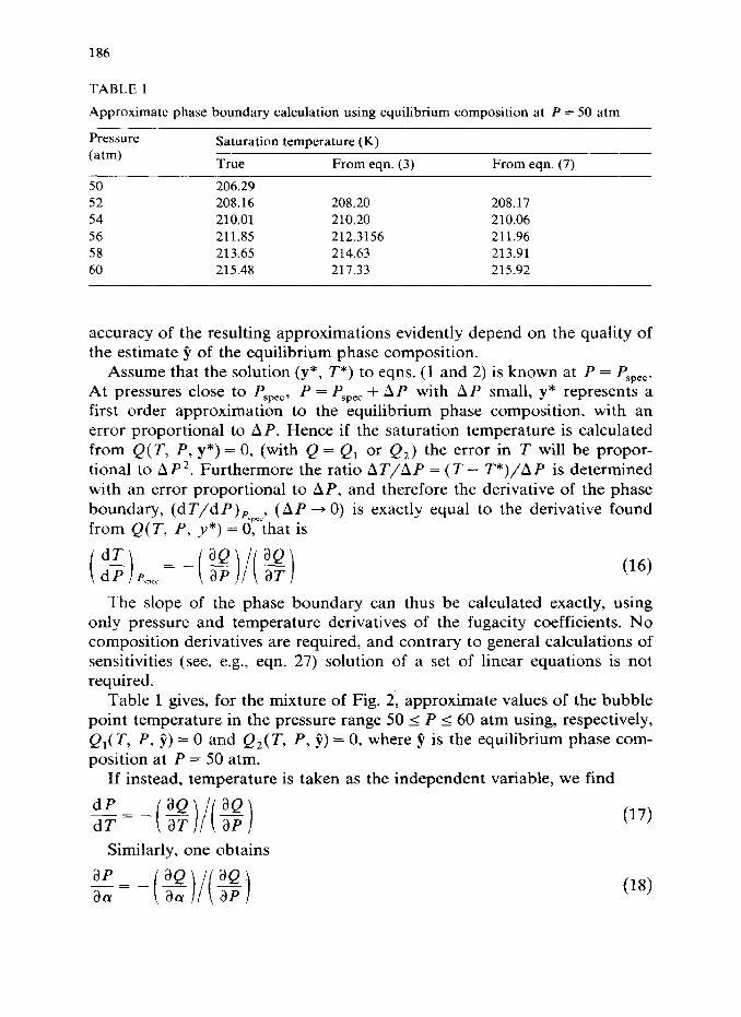
TABLE 1

Approximate phase boundary calculation using equilibrium composition at P = 50 atm

Pressure

(atm)

50 52 54 56 58 60

Saturation temperature (K)

True From eqn. (3)

206.29 208.16 208.20 210.01 210.20 211.85 212.3156 213.65 214.63 215.48 217.33

From eqn. (7)

208.17 210.06 211.96 213.91 215.92

accuracy of the resulting approximations evidently depend on the quality of the estimate y of the equilibrium phase composition.

Assume that the solution (y*, T*) to eqns. (1 and 2) is known at P = Pspec. At pressures close to Pspec, P = Pspec -t AP with A P small, y* represents a first order approximation to the equilibrium phase composition, with an error proportional to AP. Hence if the saturation temperature is calculated from Q(T, P, y*) == 0, (with Q = Q, or Q2) the error in T will be propor- tional to AP2. Furthermore the ratio AT/AP = (T - T*)/AP is determined with an error proportional to AP, and therefore the derivative of the phase boundary, (dT/dP), ., (AP-+O) from Q(T, P, y*) = drthat is

is exactly equal to the derivative found

06)

The slope of the phase boundary can thus be calculated exactly, using only pressure and temperature derivatives of the fugacity coefficients. No composition derivatives are required, and contrary to general calculations of sensitivities (see, e.g., eqn. 27) solution of a set of linear equations is not required.

Table 1 gives, for the mixture of Fig. 2, approximate values of the bubble point temperature in the pressure range 50 I P I 60 atm using, respectively, Q,( T, P, 9) = 0 and Q2( T, P, 9) = 0, where y is the equilibrium phase com- position at P = 50 atm.

If instead, temperature is taken as the independent variable, we find

dP _=- dT i

Similarly, one obtains

aQ vi 1 _- i3P 07)

187

where (Y represents any model parameter in the thermodynamic model used for evaluation of fugacity coefficients. This relation is of importance when the estimation of parameters in thermodynamic models is based on fitting calculated equilibrium pressures to measured equilibrium pressures. Each trial vector of model parameters requires saturation point calculations (at given temperature) for every set of experimental data. Once these are completed (and P and the equilibrium phase composition are available) the sensitivities of the calculated pressures to changes in the model parameters can be calculated at little extra cost using eqn. (18). The determination of such sensitivities is an integral part of all efficient parameter estimation procedures (see, e.g., Fletcher, 1980) and hence efficient evaluation is of importance.

The relation, eqn. (17), for the mixture vapour pressure has found surpris- ingly little use in phase equilibrium calculations, considering that it is well known. A similar relation for a binary mixture is, e.g., presented by Model1 and Reid (1974, Ch. 9). One possible explanation for this is that the use of a single equation of state for calculating the properties of both fluid phases has only found widespread application during the last decade. When different models are used for the fluid phases, convergence problems in bubble- and dew point calculations are largely absent, and hence there has been little incentive to improve the traditional algorithms. As discussed in the introduc- tion, when a single model is used for both fluid phases, good initial estimates are a vital necessity in saturation point calculations. It will subsequently be shown how the relations developed here can be used for providing such estimates.

TEMPERATURE AND PRESSURE MAXIMA

As can be seen from Fig. 2, the use of a single equation of state leads to a phase boundary with a pressure maximum as well as a temperature maxi- mum. The determination of these maxima is of considerable interest and construction of the entire phase boundary (Michelsen, 1980) has been suggested as an indirect method of evaluation. Equations (16) and (17), however, provide the necessary relations for a direct determination. At the temperature maximum

8Q p = 0, yielding p = 0, or <pe<

f 4 a ln e,(Y) N+2= Y,

a ln +iw = o

i ap - a~ 1

(20)

which together with eqns. (1 and 2) enables us to determine the N + 2

188

unknown (y, T, P). Similarly at the pressure maximum, eqn. (20) with temperature derivatives replacing the pressure derivatives, is used.

Newton-Raphson solution is straightforward, since essentially no new derivatives are needed. Composition derivatives of fN+Z are given by

dfhJ+, a ln+j(Y) a ln+j(z> 8 3 In +,i (Y 1 -= aYj ap -- ap

%

= a ln QY) a ln +j(4 ap -- ap

since the last term is identically zero by virtue equation.

Derivatives of fN,_2 with respect to T and P lead

(21) of the Gibbs-Duhem

to second derivatives of the type a2 In cpi/aP2 and a2 In $+/aPaT. These terms are most conveni- ently evaluated numerically, and a single calculation at a perturbed pressure is sufficient, i.e.

(22)

(23)

Apart from these only the “usual” first derivatives of fugacity coefficients with respect to composition, temperature and pressure are required.

A direct substitution procedure similar to that used for conventional saturation point calculations is also a possibility. At the current value of y the Newton correction in T and P to satisfy the two equations

is determined, and y is subsequently reevaluated from eqns. (11) and (14). Since, in particular, the pressure maximum is frequently close to the

critical point, convergence of this procedure can be slow, and divergence can occur for direct substitution as well as for the Newton-Raphson method, unless the initial estimates are close.

IMPROVED ESTIMATES

One manner of improving the approximate calculation of the phase boundary is to take into account explicitly that the equilibrium phase composition changes with changing pressure. Rather than taking jr = y*( P,,,,) one could use

ST(p) = Y*o&J + &Yk""(P - P,,.x> (29

189

With eqn. (25), the error in ji is proportional to AP*, and hence the error in T determined from Q1 or Q2 is proportional to AP4. This greatly increases the accuracy of the predictions and the range within which they yield meaningful results.

To calculate the pressure derivative of y, we note that given a solution x = x* to a set of nonlinear equations

f(x) = 0 (26)

the derivative x, of this solution with respect to a parameter of the problem is the solution to the set of linear equations

Jx, + f, = 0 (27)

where J is the Jacobian of f, .ijj = ah/ax,, and f, is the derivative of f with respect to (Y, both evaluated at x = x*.

In our case f is the set of N + 1 eqns. (1 and 2) with xT = (yr, y2, . . . yN, T), and ar is the specified pressure. If the Newton-Raphson method is used for solving the saturation point eqns. (1 and 2), J is available, and only calculation of the pressure derivatives of f are required, i.e.

af, _ a In +, (Y) _ a ln +i (Z) i = 1 2

3P ap ap 3 ,--.N (28)

and

(29)

The saturation point calculation at P = 60 atm with 9 = y*( P = 50 atm) using Q2( T, P) = 0 is in error by 0.43 K (Table 1). Compensating for the change in jr by means of eqn. (25) reduces this error to 2 X 10e4 K.

The refined estimates using a linear extrapolation for 9 can also be used for providing approximate values for the pressure and temperature maxi- mum. To determine the temperature maximum we use as a basis a dew point calculation at Pspec = 30 atm. The phase boundary obtained combining eqn. (25) with Q2(T, P) = 0 is shown in Table 2.

The correct maximum temperature is T = 255.76 K (at P = 70.06 atm), and the error of the prediction (T,,, = 255.62 K) is a modest 0.14 K even though the prediction is based on a much lower pressure. To avoid negative gi in the extrapolation, eqn. (25), In ji rather than the jz are extrapolated.

A similar approximate calculation of the pressure maximum, where 9 is taken to vary linearly with temperature, is shown in Table 3. The extrapola- tion is based on a bubble point pressure calculation at T,,, = 220 K, with P = 65.00 atm.

The true pressure maximum is P = 86.81 atm at T = 247.04 K, and we observe that a decent approximation (P = 85.8 atm) is obtained based on

190

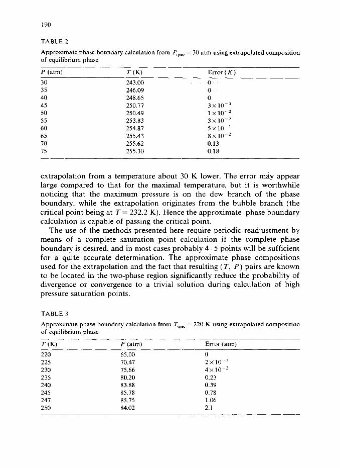
TABLE 2

Approximate phase boundary calculation from Pspec = 30 atm using extrapolated composition of equilibrium phase

P (atm) T (K) Error ( K )

30 243.00 0 35 246.09 0 40 248.65 0 45 250.77 3x1o-3 50 250.49 1x10-2 55 253.83 3x10-2 60 254.87 5x10-’ 65 255.43 8~10-~ 70 255.62 0.13 75 255.30 0.18

extrapolation from a temperature about 30 K lower. The error may appear large compared to that for the maximal temperature, but it is worthwhile noticing that the maximum pressure is on the dew branch of the phase boundary, while the extrapolation originates from the bubble branch (the critical point being at T = 232.2 K). Hence the approximate phase boundary calculation is capable of passing the critical point.

The use of the methods presented here require periodic readjustment by means of a complete saturation point calculation if the complete phase boundary is desired, and in most cases probably 4-5 points will be sufficient for a quite accurate determination. The approximate phase compositions used for the extrapolation and the fact that resulting (T, P) pairs are known to be located in the two-phase region significantly reduce the probability .of divergence or convergence to a trivial solution during calculation of high pressure saturation points.

TABLE 3

Approximate phase boundary calculation from Tsrec = 220 K using extrapolated composition of equilibrium phase

T W P (atm) Error (atm)

220 65.00 0 225 70.47 2x1o-X 230 75.66 4x10-2 235 80.20 0.23 240 83.88 0.39 245 85.78 0.78 247 85.75 1.06 250 84.02 2.1

191

An interesting possibility is to include the critical point as an anchor point for the phase boundary construction. An efficient method for location of the critical point has recently been developed (Michelsen, 1984) and this method provides as a byproduct the sensitivities needed for accurate extrapolation.

CONCLUSION

Suggestions are given for conducting simplified saturation point calcula- tions, where only a single equation is solved. These simplified calculations may be of sufficient accuracy or they may be of value as initial estimates for a complete calculation. Whether the present methods are competitive with a stepwise construction of the entire phase boundary as suggested earlier (Michelsen, 1980) remains to be seen.

LIST OF SYMBOLS

F i,j J

k

iv P

Ql

Q2 S

T f

v X

YTY* *

:

Z

error deviation function, eqns. (l-3) component indices Jacobian matrix iteration counter number of components in mixture pressure saturation point function, eqn. (3) saturation point function, eqn. (7) Jacobian matrix, eqn. (15) temperature estimate of saturation temperature deviation vector, eqn. (6) vector of independent variables equilibrium phase compositions estimate of equilibrium phase composition vector defined in eqn. (11) feed composition

Greek symbols

parameter of thermodynamic model small quantity eigenvalue fugacity coefficient, component i

192

REFERENCES

Fletcher, R., 1980. Practical methods of optimization, Vol. 1: Unconstrained optimization. John Wiley, New York.

Michelsen, M.L., 1980. Calculation of phase envelopes and critical points for multicomponent mixtures. Fluid Phase Equilibria, 4: l-10.

Michelsen, M.L., 1982. The isothermal flash problem. Part I: Stability. Fluid Phase Equi- libria, 9: l-19.

Michelsen, M.L., 1984. Calculation of critical points and of the phase boundary in the critical region. Fluid Phase Equilibria, 16: 57-76.

Modell, M. and Reid, R.C., 1974. Thermodynamics and its Applications. Prentice Hall, Englewood Cliffs, New Jersey.

Prausnitz, S., Anderson., T., Grens, E., Eckert, E., Hsieh, R. and O’Connell, J., 1980. Computer Calculations for Multicomponent Vapor-Liquid and Liquid-Liquid Equilibria. Prentice Hall, Englewood Cliffs, New Jersey.