Saturated Absorption Spectroscopy

Experiment SAS

University of Florida — Department of PhysicsPHY4803L — Advanced Physics Laboratory

Overview

You will use a tunable diode laser to carry outspectroscopic studies of the rubidium atom.You will measure the Doppler-broadened ab-sorption profiles of the D2 transitions at780 nm and then use the technique of satu-rated absorption spectroscopy to improve theresolution beyond the Doppler limit and mea-sure the nuclear hyperfine splittings, which areless than 1 ppm of the wavelength. A Fabry-Perot optical resonator is used to calibrate thefrequency scale for the measurements.Saturated absorption experiments were

cited in the 1981 Nobel prize in physics and re-lated techniques have been used in laser cool-ing and trapping experiments cited in the 1997Nobel prize as well as Bose-Einstein condensa-tion experiments cited in the 2001 Nobel prize.Although the basic principles are straightfor-ward, you will only be able to unleash the fullpower of saturated absorption spectroscopy bycarefully attending to many details.

References

1. Daryl W. Preston Doppler-free saturatedabsorption: Laser spectroscopy, Amer. J.of Phys. 64, 1432-1436 (1996).

2. K. B. MacAdam, A. Steinbach, and C.Wieman A narrow band tunable diodelaser system with grating feedback, and a

saturated absorption spectrometer for Csand Rb, Amer. J. of Phys. 60, 1098-1111(1992).

3. John C. Slater, Quantum Theory ofAtomic Structure, Vol. I, (McGraw-Hill,1960)

Theory

The purpose of this section is to outline thebasic features observed in saturated absorp-tion spectroscopy and relate them to simpleatomic and laser physics principles.

Laser interactions—two-level atom

We begin with the interactions between a laserfield and a sample of stationary atoms havingonly two possible energy levels. Aspects ofthermal motion and multilevel atoms will betreated subsequently.The difference ∆E = E1 − E0 between the

excited state energy E1 and the ground stateenergy E0 is used with Planck’s law to deter-mine the photon frequency ν associated withtransitions between the two states:

∆E = hν0 (1)

This energy-frequency proportionality is whyenergies are often given directly in frequencyunits. For example, MHz is a common energyunit for high precision laser experiments.

SAS 1

SAS 2 Advanced Physics Laboratory

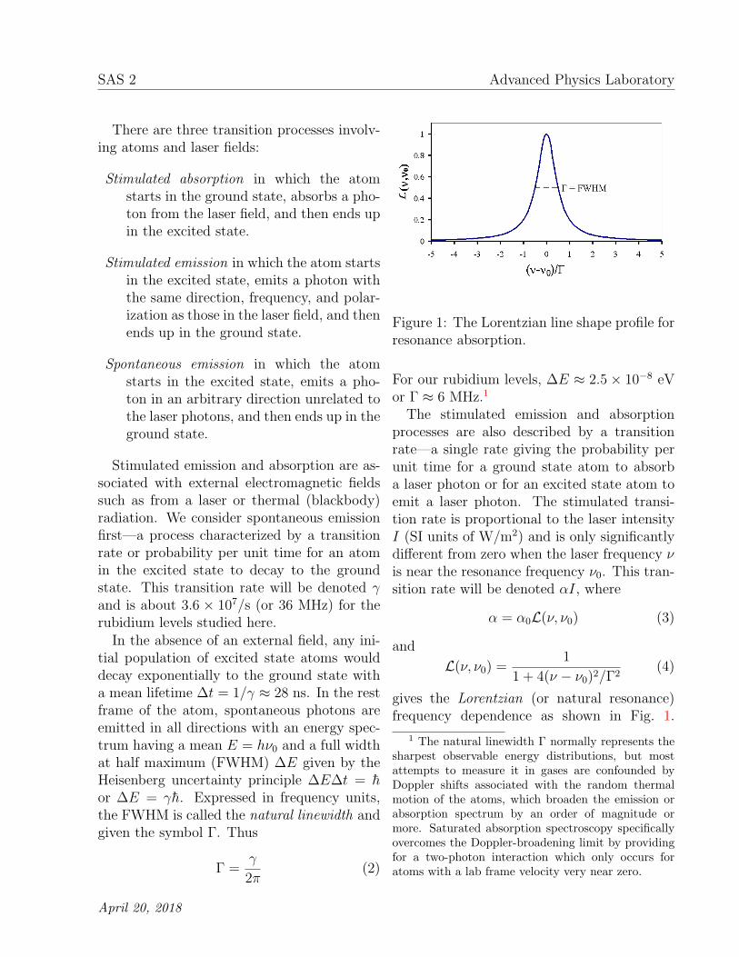
There are three transition processes involv-ing atoms and laser fields:

Stimulated absorption in which the atomstarts in the ground state, absorbs a pho-ton from the laser field, and then ends upin the excited state.

Stimulated emission in which the atom startsin the excited state, emits a photon withthe same direction, frequency, and polar-ization as those in the laser field, and thenends up in the ground state.

Spontaneous emission in which the atomstarts in the excited state, emits a pho-ton in an arbitrary direction unrelated tothe laser photons, and then ends up in theground state.

Stimulated emission and absorption are as-sociated with external electromagnetic fieldssuch as from a laser or thermal (blackbody)radiation. We consider spontaneous emissionfirst—a process characterized by a transitionrate or probability per unit time for an atomin the excited state to decay to the groundstate. This transition rate will be denoted γand is about 3.6 × 107/s (or 36 MHz) for therubidium levels studied here.In the absence of an external field, any ini-

tial population of excited state atoms woulddecay exponentially to the ground state witha mean lifetime ∆t = 1/γ ≈ 28 ns. In the restframe of the atom, spontaneous photons areemitted in all directions with an energy spec-trum having a mean E = hν0 and a full widthat half maximum (FWHM) ∆E given by theHeisenberg uncertainty principle ∆E∆t = hor ∆E = γh. Expressed in frequency units,the FWHM is called the natural linewidth andgiven the symbol Γ. Thus

Γ =γ

2π(2)

Figure 1: The Lorentzian line shape profile forresonance absorption.

For our rubidium levels, ∆E ≈ 2.5× 10−8 eVor Γ ≈ 6 MHz.1

The stimulated emission and absorptionprocesses are also described by a transitionrate—a single rate giving the probability perunit time for a ground state atom to absorba laser photon or for an excited state atom toemit a laser photon. The stimulated transi-tion rate is proportional to the laser intensityI (SI units of W/m2) and is only significantlydifferent from zero when the laser frequency νis near the resonance frequency ν0. This tran-sition rate will be denoted αI, where

α = α0L(ν, ν0) (3)

and

L(ν, ν0) =1

1 + 4(ν − ν0)2/Γ2(4)

gives the Lorentzian (or natural resonance)frequency dependence as shown in Fig. 1.

1 The natural linewidth Γ normally represents thesharpest observable energy distributions, but mostattempts to measure it in gases are confounded byDoppler shifts associated with the random thermalmotion of the atoms, which broaden the emission orabsorption spectrum by an order of magnitude ormore. Saturated absorption spectroscopy specificallyovercomes the Doppler-broadening limit by providingfor a two-photon interaction which only occurs foratoms with a lab frame velocity very near zero.

April 20, 2018

Saturated Absorption Spectroscopy SAS 3

laserbeam

photodiodevapor cell

Figure 2: Basic arrangement for ordinary laserabsorption spectroscopy.

L(ν, ν0) also describes the spectrum of radia-tion from spontaneous emission and the widthΓ is the same for both cases. The maximumtransition rate α0I occurs right on resonance(ν = ν0) and for the rubidium transitionsstudied here α0 ≈ 2× 106m2/J.The value of γ/α0 defines a parameter of the

atoms called the saturation intensity Isat

Isat =γ

α0

(5)

and is about 1.6 mW/cm2 for our rubidiumtransitions.2 Its significance is that when thelaser intensity is equal to the saturation in-tensity, excited state atoms are equally likelyto decay by stimulated emission or by sponta-neous emission.

Basic laser absorption spectroscopy

The basic arrangement for ordinary laserabsorption (not saturated absorption) spec-troscopy through a gaseous sample is shownin Fig. 2. A laser beam passes through thevapor cell and its intensity is measured by aphotodiode detector as the laser frequency νis scanned through the natural resonance fre-quency.When a laser beam propagates through a

gaseous sample, the two stimulated transi-tion processes change the intensity of the laser

2 γ, Γ, α0, Isat vary somewhat among the vari-ous rubidium D2 transitions studied here. The valuesgiven are only representative.

beam and affect the density of atoms (num-ber per unit volume) in the ground and ex-cited states. Moreover, Doppler shifts associ-ated with the random thermal motion of theabsorbing atoms must also be taken into ac-count. There is an interplay among these ef-fects which is critical to understanding satu-rated absorption spectroscopy. We begin withthe basic equation describing how the laser in-tensity changes as it propagates through thesample and then continue with the effects ofDoppler shifts and population changes.

Laser absorption

Because of stimulated emission and absorp-tion, the laser intensity I(x) varies as it prop-agates from x to x+ dx in the medium.

Exercise 1 Show that

I(x+ dx)− I(x) = −hναI(x)(P0 − P1)n0dx(6)

Hints: Multiply both sides by the laser beamcross sectional area A and use conservation ofenergy. Keeping in mind that I(x) is the laserbeam intensity at some position x inside thevapor cell, explain what the left side would rep-resent. With n0 representing the overall den-sity of atoms (number per unit volume) in thevapor cell, what does n0Adx represent? P0 andP1 represent the probabilities that the atomsare in the ground and excited states, respec-tively, or the fraction of atoms in each state.They can be assumed to be given. What thenis the rate at which atoms undergo stimulatedabsorption and stimulated emission? Finally,recall that hν is the energy of each photon. Sowhat would the right side represent?

Equation 6 leads to

dI

dx= −κI (7)

April 20, 2018

SAS 4 Advanced Physics Laboratory

where the absorption coefficient (fractional ab-sorption per unit length)

κ = hνn0α(P0 − P1) (8)

The previous exercise demonstrates that theproportionality to P0 − P1 arises from thecompetition between stimulated emission andabsorption and it is important to appreciatethe consequences. If there are equal num-bers of atoms in the ground and excited state(P0 − P1 = 0), laser photons are as likely tobe emitted by an atom in the excited stateas they are to be absorbed by an atom in theground state and there will be no attenuationof the incident beam. The attenuation maxi-mizes when all atoms are in the ground state(P0−P1 = 1) because only upward transitionswould be possible. And the attenuation caneven reverse sign (become an amplification asit does in laser gain media) if there are moreatoms in the excited state (P1 > P0).In the absence of a laser field, the ratio

of the atomic populations in the two energystates will thermally equilibrate at the Boltz-mann factor P1/P0 = e−∆E/kT = e−hν0/kT . Atroom temperature, kT (≈ 1/40 eV) is muchsmaller than the hν0 (≈ 1.6 eV) energy dif-ference for the levels involved in this exper-iment and nearly all atoms will be in theground state, i.e., P0 − P1 = 1. While youwill see shortly how the presence of a stronglaser field can significantly perturb these ther-mal equilibrium probabilities, for now we willonly treat the case where the laser field is weakenough that P0 − P1 = 1 remains a good ap-proximation throughout the absorption cell.

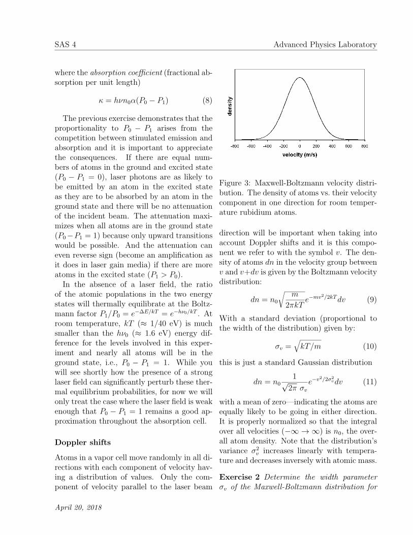
Doppler shifts

Atoms in a vapor cell move randomly in all di-rections with each component of velocity hav-ing a distribution of values. Only the com-ponent of velocity parallel to the laser beam

Figure 3: Maxwell-Boltzmann velocity distri-bution. The density of atoms vs. their velocitycomponent in one direction for room temper-ature rubidium atoms.

direction will be important when taking intoaccount Doppler shifts and it is this compo-nent we refer to with the symbol v. The den-sity of atoms dn in the velocity group betweenv and v+dv is given by the Boltzmann velocitydistribution:

dn = n0

√m

2πkTe−mv2/2kTdv (9)

With a standard deviation (proportional tothe width of the distribution) given by:

σv =√kT/m (10)

this is just a standard Gaussian distribution

dn = n01√

2π σv

e−v2/2σ2vdv (11)

with a mean of zero—indicating the atoms areequally likely to be going in either direction.It is properly normalized so that the integralover all velocities (−∞ → ∞) is n0, the over-all atom density. Note that the distribution’svariance σ2

v increases linearly with tempera-ture and decreases inversely with atomic mass.

Exercise 2 Determine the width parameterσv of the Maxwell-Boltzmann distribution for

April 20, 2018

Saturated Absorption Spectroscopy SAS 5

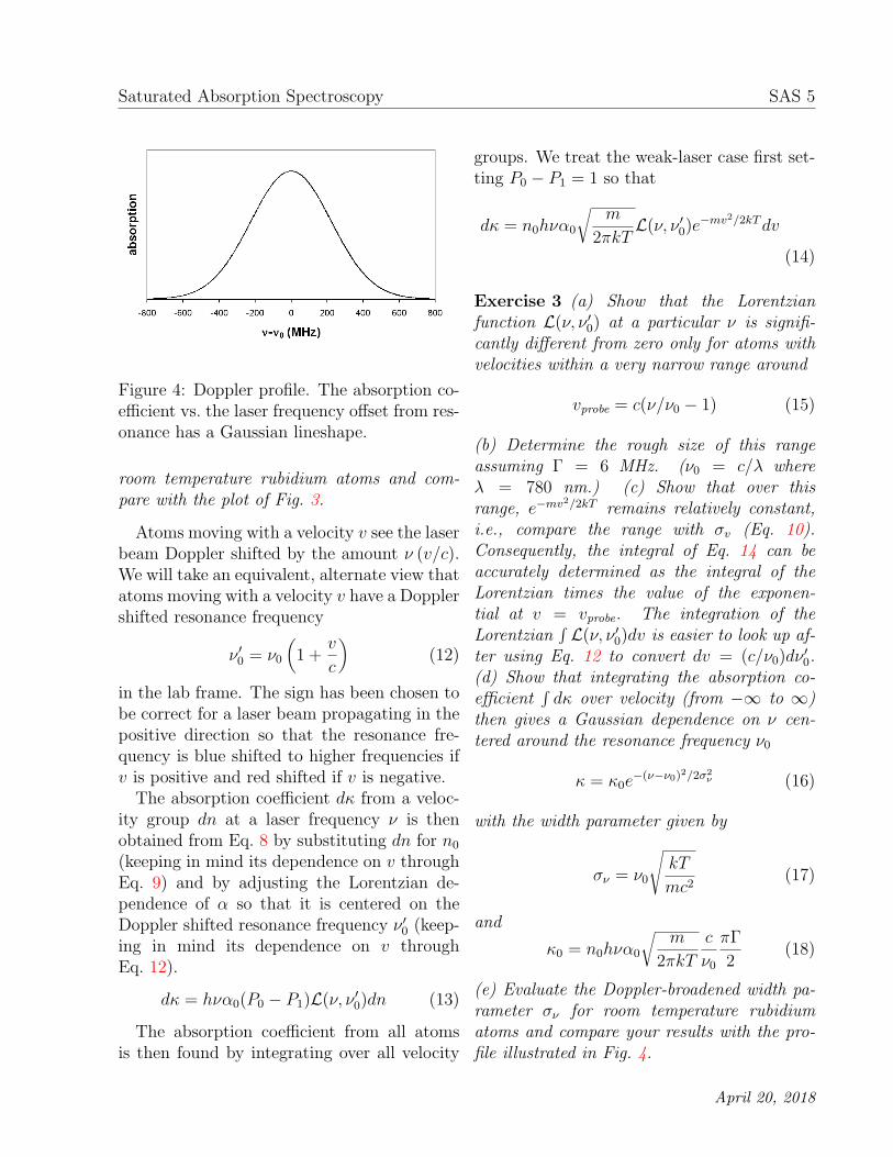
Figure 4: Doppler profile. The absorption co-efficient vs. the laser frequency offset from res-onance has a Gaussian lineshape.

room temperature rubidium atoms and com-pare with the plot of Fig. 3.

Atoms moving with a velocity v see the laserbeam Doppler shifted by the amount ν (v/c).We will take an equivalent, alternate view thatatoms moving with a velocity v have a Dopplershifted resonance frequency

ν ′0 = ν0

(1 +

v

c

)(12)

in the lab frame. The sign has been chosen tobe correct for a laser beam propagating in thepositive direction so that the resonance fre-quency is blue shifted to higher frequencies ifv is positive and red shifted if v is negative.The absorption coefficient dκ from a veloc-

ity group dn at a laser frequency ν is thenobtained from Eq. 8 by substituting dn for n0

(keeping in mind its dependence on v throughEq. 9) and by adjusting the Lorentzian de-pendence of α so that it is centered on theDoppler shifted resonance frequency ν ′

0 (keep-ing in mind its dependence on v throughEq. 12).

dκ = hνα0(P0 − P1)L(ν, ν ′0)dn (13)

The absorption coefficient from all atomsis then found by integrating over all velocity

groups. We treat the weak-laser case first set-ting P0 − P1 = 1 so that

dκ = n0hνα0

√m

2πkTL(ν, ν ′

0)e−mv2/2kTdv

(14)

Exercise 3 (a) Show that the Lorentzianfunction L(ν, ν ′

0) at a particular ν is signifi-cantly different from zero only for atoms withvelocities within a very narrow range around

vprobe = c(ν/ν0 − 1) (15)

(b) Determine the rough size of this rangeassuming Γ = 6 MHz. (ν0 = c/λ whereλ = 780 nm.) (c) Show that over thisrange, e−mv2/2kT remains relatively constant,i.e., compare the range with σv (Eq. 10).Consequently, the integral of Eq. 14 can beaccurately determined as the integral of theLorentzian times the value of the exponen-tial at v = vprobe. The integration of theLorentzian

∫L(ν, ν ′

0)dv is easier to look up af-ter using Eq. 12 to convert dv = (c/ν0)dν

′0.

(d) Show that integrating the absorption co-efficient

∫dκ over velocity (from −∞ to ∞)

then gives a Gaussian dependence on ν cen-tered around the resonance frequency ν0

κ = κ0e−(ν−ν0)2/2σ2

ν (16)

with the width parameter given by

σν = ν0

√kT

mc2(17)

and

κ0 = n0hνα0

√m

2πkT

c

ν0

πΓ

2(18)

(e) Evaluate the Doppler-broadened width pa-rameter σν for room temperature rubidiumatoms and compare your results with the pro-file illustrated in Fig. 4.

April 20, 2018

SAS 6 Advanced Physics Laboratory

Populations

Now we would like to take into account thechanges to the ground and excited state pop-ulations arising from a laser beam propagat-ing through the cell. The rate equations forthe ground and excited state probabilities orfractions become:

dP0

dt= γP1 − αI(P0 − P1)

dP1

dt= −γP1 + αI(P0 − P1) (19)

where the first term on the right in each equa-tion arises from spontaneous emission and thesecond term arises from stimulated absorptionand emission.

Exercise 4 (a) Show that steady state condi-tions (i.e., where dP0/dt = dP1/dt = 0) leadto probabilities satisfying

P0 − P1 =1

1 + 2αI/γ(20)

Hint: You will also need to use P0 + P1 = 1.(b) Show that when this result is used in Eq. 8(for stationary atoms) and the frequency de-pendence of α as given by Eqs. 3-4 is also in-cluded, the absorption coefficient κ again takesthe form of a Lorentzian

κ =hνn0α0

1 + 2I/IsatL′(ν, ν0) (21)

where L′ is a standard Lorentzian

L′(ν, ν0) =1

1 + 4(ν − ν0)2/Γ′2 (22)

with a power-broadened width parameter

Γ′ = Γ√1 + 2I/Isat (23)

The approach to the steady state probabili-ties is exponential with a time constant around

[γ+2αI]−1, which is less than 28 ns for our ru-bidium transitions. Thus as atoms, mostly inthe ground state, wander into the laser beamat thermal velocities, they would only travel afew microns before reaching equilibrium prob-abilities.

C.Q. 1 Take into account velocity groups andtheir corresponding Doppler shifts for the caseP0 − P1 = 1. The calculation is performedas in Exercise 3. Show that the result afterintegrating over all velocity groups is:

κ = κ′0e

−(ν−ν0)2/2σ2ν (24)

where the width parameter, σν is the same asbefore (Eq. 17), but compared to the weak-fieldabsorption coefficient (Eq. 18), the strong-fieldcoefficient decreases to

κ′0 =

κ0√1 + 2I/Isat

(25)

Laser absorption through a cell

In the weak-field case κ at any frequency isgiven by Eq. 16 (with Eq. 18) and is indepen-dent of the laser intensity. In this case, Eq. 7is satisfied by Beer’s law which says that theintensity decays exponentially with distancetraveled through the sample.

I(x) = I0e−κx (26)

In the general case, κ is given by Eq. 24(with Eq. 25) and at any frequency is propor-

tional to 1/√1 + 2I/Isat. The general solution

to Eq. 7 for how the laser intensity varies withthe distance x into the cell is then rather morecomplicated than Beer’s law and is given inan appendix that can be found on the lab website. However, the strong-field I >> Isat be-havior is easily determined by neglecting the1 compared to I/Isat so that Eq. 7 becomes

dI

dx= −k

√I (27)

April 20, 2018

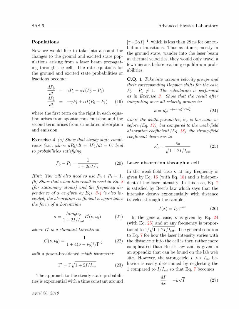
Saturated Absorption Spectroscopy SAS 7

probebeam

pumpbeam

photodiodevapor cell

Figure 5: Basic arrangement for saturated ab-sorption spectroscopy.

where

k = κ0

√Isat/2e

−(ν−ν0)2/2σ2ν (28)

Saturated absorption—simple model

Up to now, we have considered only a singlelaser beam propagating through the cell. Nowwe would like to understand what happenswhen a second laser propagates through thecell in the opposite direction. This is the ba-sic arrangement for saturated absorption spec-troscopy shown in Fig. 5. The laser beamtraveling to the right—the one we have beenconsidering up to now and whose absorptionis measured—is now called the probe beam.The second overlapping laser beam propagat-ing in the opposite direction is called the pumpbeam. Both beams will be from the same laserand so they will have the same frequency, evenas that frequency is scanned through the res-onance.With only a single weak laser propagat-

ing through the sample, P0 − P = 1 wouldbe a good approximation throughout the cell.With the two beams propagating through thecell, the probe beam will still be kept weak—weak enough to neglect its affect on the pop-ulations. However, the pump beam will bemade strong—strong enough to significantlyaffect the populations and thus change themeasured absorption of the probe beam. Tounderstand how this comes about, we willagain have to consider Doppler shifts.

As mentioned, the stimulated emission andabsorption rates are nonzero only when thelaser is near the resonance frequency. Thus,we will obtain P0−P1 from Eq. 20 by giving α aLorentzian dependence on the Doppler shiftedresonance frequency:

α = α0L(ν, ν ′′0 ) (29)

with the important feature that for the pumpbeam, the resonance frequency for atoms mov-ing with a velocity v is

ν ′′0 = ν0

(1− v

c

)(30)

This frequency is Doppler shifted in the direc-tion opposite that of the probe beam becausethe pump beam propagates through the vaporcell in the negative direction. That is, the res-onant frequency for an atom moving with asigned velocity v is ν0(1 + v/c) for the probebeam and ν0(1− v/c) for the pump beam.

Exercise 5 (a) Plot Eq. 20 versus the detun-ing parameter

δ = ν − ν ′′0 (31)

for values of I/Isat from 0.1 to 1000. (Use Γ =6 MHz.) (b) Use your graphs to determine howthe FWHM of the dips in P0−P1 change withlaser power.

Exercise 5 should have demonstrated thatfor large detunings (δ ≫ Γ), P0 − P1 = 1 im-plying that in this case the atoms are in theground state—the same as when there is nopump beam. On resonance, i.e., at δ = 0,P0 − P1 = 1/(1 + 2I/Isat), which approacheszero for large values of I. This implies thatatoms in resonance with a strong pump beamwill have equal populations in the ground andexcited states (P0−P1 = 0). That is, a strong,

April 20, 2018

SAS 8 Advanced Physics Laboratory

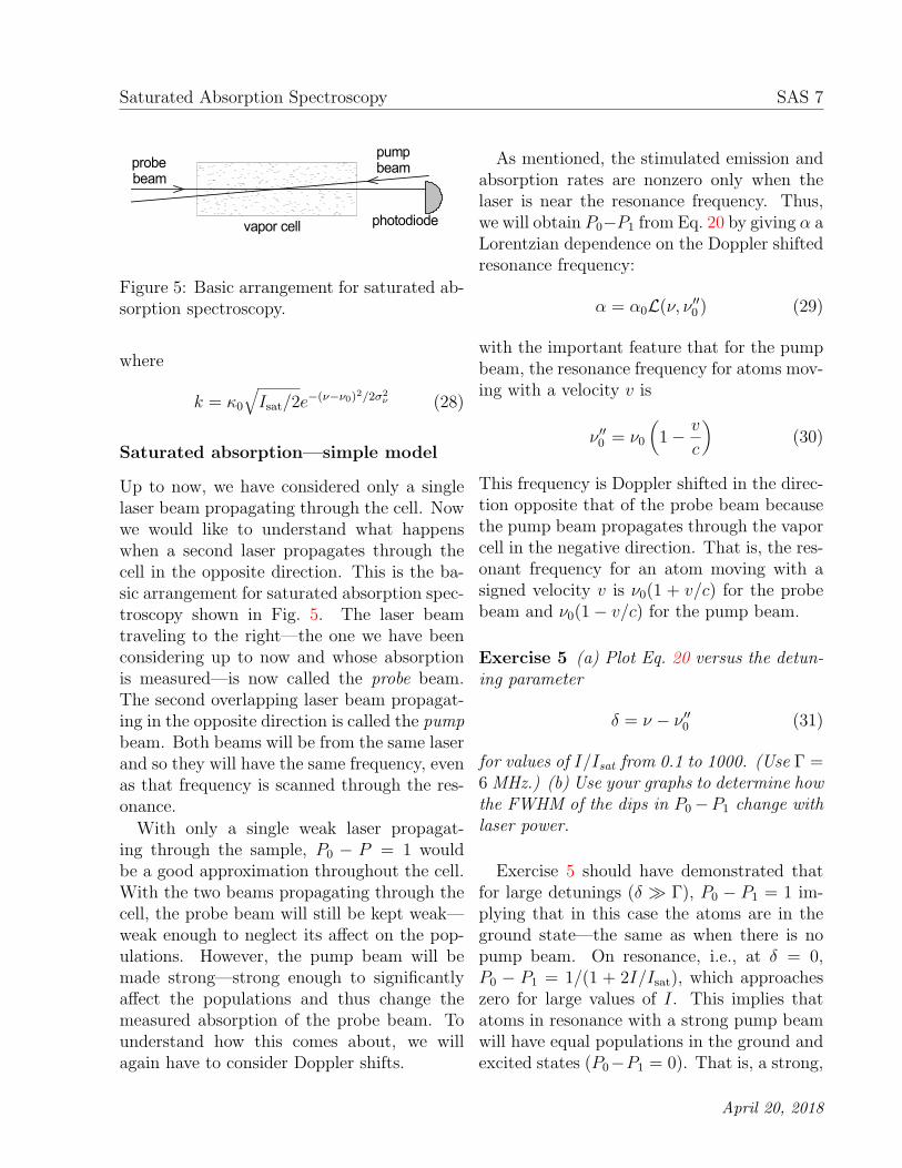
Figure 6: Hole burning by the pump beam.The density of ground state atoms is plottedvs. their velocity and becomes depleted nearthe velocity that Doppler shifts the laser fre-quency into resonance with ν0.

resonant laser field causes such rapid transi-tions in both directions that the two popula-tions equilibrate. The laser is said to “satu-rate” the transition, which is the origin of thename of the technique.According to Eq. 30, the resonance condi-

tion (δ = 0) translates to v = vpump where

vpump = c(1− ν/ν0) (32)

Consequently, for any frequency ν within theDoppler profile, only atoms near this veloc-ity will be at zero detuning and will have val-

ues of P0−P1 perturbed from the “pump off”value of unity. Of course, whether there area significant number of atoms in either levelnear v = vpump depends on the width of theBoltzmann velocity distribution and the rela-tive values of ν and ν0. But if vpump is withinthe distribution, the atoms near that velocitywill have perturbed populations.

The density of atoms in the ground statedn1 = P1 dn plotted as a function of v will fol-low the Maxwell-Boltzmann distribution ex-cept very near v = vpump where it will dropoff significantly as atoms are promoted to theexcited state. This is called “hole burning”as there is a hole (a decrease) in the densityof atoms in the ground state near v = vpump

(and a corresponding increase in the density ofatoms in the excited state) as demonstrated inFig. 6.

How does hole burning affect the probebeam absorption? In Exercise 3 you learnedthat the absorption at any frequency ν arisesonly from those atoms moving with veloc-ities near vprobe = c(ν/ν0 − 1). Also re-call, the probe beam absorption is propor-tional to P0 − P1, which we have just seenremains constant (≈ 1) except for atoms hav-ing nearly the exact opposite velocities nearvpump = c(1 − ν/ν0). Therefore, when thelaser frequency is far from the natural reso-nance (|ν − ν0| ≫ Γ), the probe absorptionarises from atoms moving with a particular ve-locity in one direction while the pump beam isburning a hole for a completely different set ofatoms with the opposite velocity. In this case,the presence of the pump beam will not affectthe probe beam absorption which would followthe standard Doppler-broadened profile.

Only when the laser frequency is very nearthe resonance frequency (ν = ν0, vprobe =vpump = 0) will the pump beam burn a hole foratoms with velocities near zero which wouldthen be the same atoms involved with the

April 20, 2018

Saturated Absorption Spectroscopy SAS 9

Figure 7: Absorption coefficient vs. the laserfrequency offset from resonance for a two-levelatom at values of I/Isat = 0.1, 1, 10, 100, 1000(from smallest dip to largest). It shows aGaussian profile with the saturated absorptiondip at ν = ν0.

probe beam absorption at this frequency. Theabsorption coefficient would be obtained bytaking P1−P0 as given by Eq. 20 (with Eqs. 29and 30) to be a function of the laser frequencyν and the velocity v, using it in Eq. 13 (withEqs. 9 and 12), and then integrating over ve-locity. The result is a Doppler-broadened pro-file with what’s called a saturated absorptiondip (or Lamb dip) right at ν = ν0. Numeri-cal integration was used to create the profilesshown in Fig. 7 for several values of I/Isat.

Multilevel effects

Real atoms have multiple upper and lowerenergy levels which add complexities to thesimple two-level model presented so far. Forthis experiment, transitions between two lowerlevels and four upper levels can all bereached with our laser and add features calledcrossover resonances and a process called op-tical pumping. Crossover resonance are addi-

0

1

2

V-system

0

1

2

Λ-systemE

hν2hν1 hν1

hν0

Figure 8: Energy levels for two possible three-level systems. The V-configuration with twoupper levels and the) Λ-system with two lowerlevels.

tional narrow absorption dips arising becauseseveral upper or lower levels are close enoughin energy that their Doppler-broadened pro-files overlap. Optical pumping occurs whenthe excited level can spontaneously decay tomore than one lower level. It can significantlydeplete certain ground state populations fur-ther enhancing or weakening the saturated ab-sorption dips.

The basics of crossover resonances can beunderstood within the three-level atom in ei-ther the Λ- or V-configurations shown in Fig. 8where the arrows represent allowed sponta-neous and stimulated transitions. In this ex-periment, crossover resonances arise from mul-tiple upper levels and so we will illustrate withthe V-system. Having two excited energy lev-els 1 and 2, the resonance frequencies to theground state 0 are ν1 and ν2, which are as-sumed to be spaced less than a Doppler widthapart.

Without the pump beam, each excited statewould absorb with a Doppler-broadened pro-file and the net absorption would be the sum oftwo Gaussian profiles, one centered at ν1 and

April 20, 2018

SAS 10 Advanced Physics Laboratory

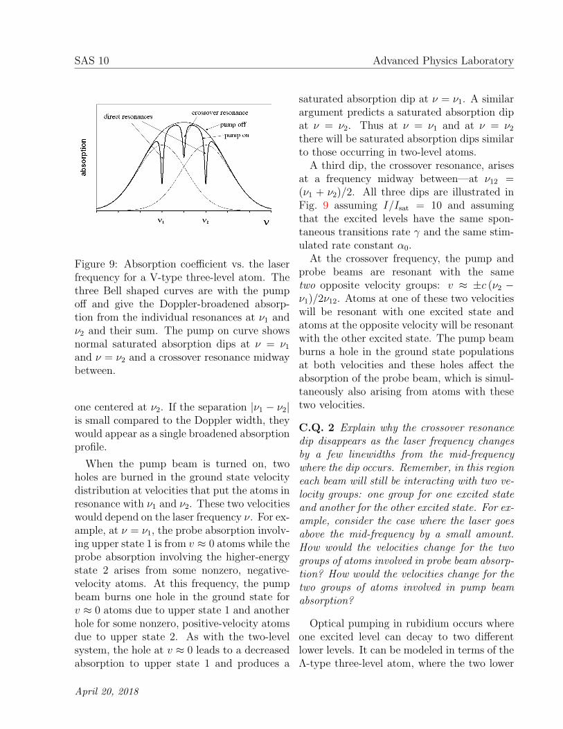
Figure 9: Absorption coefficient vs. the laserfrequency for a V-type three-level atom. Thethree Bell shaped curves are with the pumpoff and give the Doppler-broadened absorp-tion from the individual resonances at ν1 andν2 and their sum. The pump on curve showsnormal saturated absorption dips at ν = ν1and ν = ν2 and a crossover resonance midwaybetween.

one centered at ν2. If the separation |ν1 − ν2|is small compared to the Doppler width, theywould appear as a single broadened absorptionprofile.

When the pump beam is turned on, twoholes are burned in the ground state velocitydistribution at velocities that put the atoms inresonance with ν1 and ν2. These two velocitieswould depend on the laser frequency ν. For ex-ample, at ν = ν1, the probe absorption involv-ing upper state 1 is from v ≈ 0 atoms while theprobe absorption involving the higher-energystate 2 arises from some nonzero, negative-velocity atoms. At this frequency, the pumpbeam burns one hole in the ground state forv ≈ 0 atoms due to upper state 1 and anotherhole for some nonzero, positive-velocity atomsdue to upper state 2. As with the two-levelsystem, the hole at v ≈ 0 leads to a decreasedabsorption to upper state 1 and produces a

saturated absorption dip at ν = ν1. A similarargument predicts a saturated absorption dipat ν = ν2. Thus at ν = ν1 and at ν = ν2there will be saturated absorption dips similarto those occurring in two-level atoms.A third dip, the crossover resonance, arises

at a frequency midway between—at ν12 =(ν1 + ν2)/2. All three dips are illustrated inFig. 9 assuming I/Isat = 10 and assumingthat the excited levels have the same spon-taneous transitions rate γ and the same stim-ulated rate constant α0.At the crossover frequency, the pump and

probe beams are resonant with the sametwo opposite velocity groups: v ≈ ±c (ν2 −ν1)/2ν12. Atoms at one of these two velocitieswill be resonant with one excited state andatoms at the opposite velocity will be resonantwith the other excited state. The pump beamburns a hole in the ground state populationsat both velocities and these holes affect theabsorption of the probe beam, which is simul-taneously also arising from atoms with thesetwo velocities.

C.Q. 2 Explain why the crossover resonancedip disappears as the laser frequency changesby a few linewidths from the mid-frequencywhere the dip occurs. Remember, in this regioneach beam will still be interacting with two ve-locity groups: one group for one excited stateand another for the other excited state. For ex-ample, consider the case where the laser goesabove the mid-frequency by a small amount.How would the velocities change for the twogroups of atoms involved in probe beam absorp-tion? How would the velocities change for thetwo groups of atoms involved in pump beamabsorption?

Optical pumping in rubidium occurs whereone excited level can decay to two differentlower levels. It can be modeled in terms of theΛ-type three-level atom, where the two lower

April 20, 2018

Saturated Absorption Spectroscopy SAS 11

levels are separated in energy by much morethan a Doppler width.

Assume the laser beam is resonant withatoms in only one of the lower levels, butatoms in the excited level spontaneously de-cay to either lower level more or less equally.Then, each time an atom in the “resonant”lower level is promoted by the laser to the ex-cited level, some fraction of the time it willdecay to the “non-resonant” lower level. Oncein the non-resonant lower level, the atom nolonger interacts with the laser field. It be-comes “shelved” and unable to contribute tothe absorption. Analysis of the level popula-tions then requires a model where atoms out-side the laser beam interaction volume ran-domly diffuse back into it thereby replenishingthe resonant lower level populations. Depend-ing on the laser intensity and beam geometry,the lower level populations can be significantlyaltered by optical pumping.

As with the population variations arisingfrom stimulated emission and absorption, op-tical pumping also depends on the laser fre-quency and atom velocities. Optical pumpingdue to the pump beam can drastically depleteresonant ground state atoms and can signif-icantly increase the size of the saturated ab-sorption dips. Optical pumping due to theprobe beam can also affect saturated absorp-tion measurements, particularly if the probelaser intensity is high. In this case, the probebeam shelves the atoms involved in the ab-sorption at all frequencies, not just at the sat-urated absorption dips.

Surprisingly, optical pumping does not sig-nificantly change the predicted form for theabsorption signals. Largely, its effect is tochange the widths (Γ’s), the saturation inten-sities (Isat’s) and the strengths (κ’s) appearingin the formulae.

Energy levels in rubidium

One common application of saturated absorp-tion spectroscopy is in measuring the hyper-fine splittings of atomic spectral lines. Theyare so small that Doppler broadening normallymakes it impossible to resolve them. Youwill use saturated absorption spectroscopy tostudy the hyperfine splittings in the rubidiumatom and thus will need to know a little aboutits energy level structure.In principle, quantum mechanical calcula-

tions can accurately predict the energy levelsand electronic wavefunctions of multielectronatoms. In practice, the calculations are diffi-cult and this section will only present enoughof the results to appreciate the basic structureof rubidium’s energy levels. You should con-sult the references for a more in-depth treat-ment of the topic.The crudest treatment of the energy lev-

els in multielectron atoms is called the centralfield approximation (CFA). In this approxima-tion the nuclear and electron magnetic mo-ments are ignored and the atomic electronsare assumed to interact, not with each other,but with an effective radial electric field aris-ing from the average charge distribution fromthe nucleus and all the other electrons in theatom.Solving for the energy levels in the CFA

leads to an atomic configuration in which eachelectron is described by the following quantumnumbers:

1. The principal quantum number n (al-lowed integer values greater than zero)characterizes the radial dependence of thewavefunction.

2. The orbital angular momentum quantumnumber ℓ (allowed values from 0 to n −1) characterizes the angular dependenceof the wavefunction and the magnitude

April 20, 2018

SAS 12 Advanced Physics Laboratory

of the orbital angular momentum ℓ of anindividual electron.3

3. The magnetic quantum number mℓ (al-lowed values from −ℓ to ℓ) further char-acterizes the angular dependence of thewavefunction and the projection of ℓ on achosen quantization axis.4

4. The electron spin quantum number s(only allowed value equal to 1/2) charac-terizes the magnitude of the intrinsic orspin angular momentum s of an individ-ual electron.

5. The spin projection quantum number ms

(allowed values ±1/2) characterizes theprojection of s on a chosen quantizationaxis.

The rubidium atom (Rb) has atomic num-ber 37. In its lowest (ground state) config-uration it has one electron outside an inertgas (argon) core and is described with the no-tation 1s22s22p63s23p63d104s24p65s. The inte-gers 1 through 5 above specify principal quan-tum numbers n. The letters s, p, and d specifyorbital angular momentum quantum numbersℓ as 0, 1, and 2, respectively. The superscriptsindicate the number of electrons with thosevalues of n and ℓ.

The Rb ground state configuration is saidto have filled shells to the 4p orbitals and asingle valence (or optical) electron in a 5s or-bital. The next higher energy configurationhas the 5s valence electron promoted to a 5porbital with no change to the description ofthe remaining 36 electrons.

3 Angular momentum operators such as ℓ satisfyan eigenvalue equation of the form ℓ2ψ = ℓ(ℓ+1)h2ψ.

4 Angular momentum projection operators such asℓz satisfy an eigenvalue equation of the form ℓzψ =mℓhψ.

Fine structure levels

Within a configuration, there can be severalfine structure energy levels differing in the en-ergy associated with the coulomb and spin-orbit interactions. The coulomb interaction isassociated with the normal electrostatic po-tential energy kq1q2/r12 between each pair ofelectrons and between each electron and thenucleus. (Most, but not all of the coulomb in-teraction energy is included in the configura-tion energy.) The spin-orbit interaction is as-sociated with the orientation energy −µ ·B ofthe magnetic dipole moment µ of each electronin the internal magnetic field B of the atom.The form and strength of these two interac-tions in rubidium are such that the energylevels are most accurately described in the L-S or Russell-Saunders coupling scheme. L-Scoupling introduces new angular momentumquantum numbers L, S, and J as describednext.

1. L is the quantum number describing themagnitude of the total orbital angularmomentum L, which is the sum of theorbital angular momentum of each elec-tron:

L =∑

ℓi (33)

2. S is the quantum number describing themagnitude of the total electronic spin an-gular momentum S, which is the sum ofthe spin angular momentum of each elec-tron:

S =∑

si (34)

3. J is the quantum number describing themagnitude of the total electronic angularmomentum J, which is the sum of the to-tal orbital and total spin angular momen-tum:

J = L+ S (35)

April 20, 2018

Saturated Absorption Spectroscopy SAS 13

The values for L and S and J are specifiedin a notation (2S+1)LJ invented by early spec-troscopists. The letters S, P, and D (as withthe letters s, p, and d for individual electrons)are used for L and correspond to L = 0, 1,and 2, respectively. The value of (2S + 1) iscalled the multiplicity and is thus 1 for S = 0and called a singlet, 2 for S = 1/2 (doublet),3 for S = 1 (triplet), etc. The value of J (withallowed values from |L−S| to L+S) is anno-tated as a subscript to the value of L.5

The sum of ℓi or si over all electrons inany filled orbital is always zero. Thus for Rbconfigurations with only one valence electron,there is only one allowed value for L and S:just the value of ℓi and si for that electron.In its ground state (5s) configuration, Rb isdescribed by L = 0 and S = 1/2. The onlypossible value for J is then 1/2 and the finestructure state would be labeled 2S1/2. Itsnext higher (5p) configuration is described byL = 1 and S = 1/2. In this configurationthere are two allowed values of J : 1/2 and 3/2and these two fine structure states are labeled2P1/2 and 2P3/2.

Hyperfine levels

Within each fine structure level there can bean even finer set of hyperfine levels differing inthe orientation energy (again, a −µ · B typeenergy) associated with the nuclear magneticmoment in the magnetic field of the atom.The nuclear magnetic moment is much smaller

5 The terms singlet, doublet, triplet etc. are associ-ated with the number of allowed values of J typicallypossible with a given L and S (if L ≥ S). Historically,the terms arose from the number of closely-spacedspectral lines typically (but not always) observed inthe decay of these levels. For example, the sodiumdoublet at 589.0 and 589.6 nm occurs in the decay ofthe 2P1/2 and 2P3/2 fine structure levels to the 2S1/2ground state. While the 2P1/2 and 2P3/2 are truly adoublet of closely-spaced energy levels, the 2S1/2 statehas only one allowed value of J .

than the electron magnetic moment and this iswhy the hyperfine splittings are so small. Thenuclear magnetic moment is proportional tothe spin angular momentum I of the nucleus,whose magnitude is described by the quantumnumber I. Allowed values for I depend on nu-clear structure and vary with the isotope.The hyperfine energy levels depend on the

the total angular momentum F of the atom:the sum of the total electron angular momen-tum J and the nuclear spin angular momen-tum I:

F = J+ I (36)

The magnitude of F is characterized by thequantum number F with allowed values from|J − I| to J + I. Each state with a differentvalue of F will have a slightly different energydue to the interaction of the nuclear magneticmoment and the internal field of the atom.There is no special notation for the labelingof hyperfine states and F is usually labeledexplicitly in energy level diagrams.There are two naturally occurring isotopes

of Rb: 72% abundant 87Rb with I = 3/2and 28% abundant 85Rb with I = 5/2. Forboth isotopes, this leads to two hyperfine lev-els within the 2S1/2 and 2P1/2 fine structurelevels (F = I−1/2 and F = I+1/2) and fourhyperfine levels within the 2P3/2 fine structurelevel (F = I − 3/2, I − 1/2, I +1/2, I +3/2).The energies of the hyperfine levels can be

expressed (relative to a “mean” energy EJ forthe fine structure state) in terms of two hyper-fine constants A and B by the Casimir formula

EF = EJ + Aκ

2(37)

+ B3κ(κ+ 1)/4− I(I + 1)J(J + 1)

2I(2I − 1)J(2J − 1)

where κ = F (F +1)− J(J +1)− I(I +1). (Ifeither I = 1/2 or J = 1/2, the term containingB must be omitted.)

April 20, 2018

SAS 14 Advanced Physics Laboratory

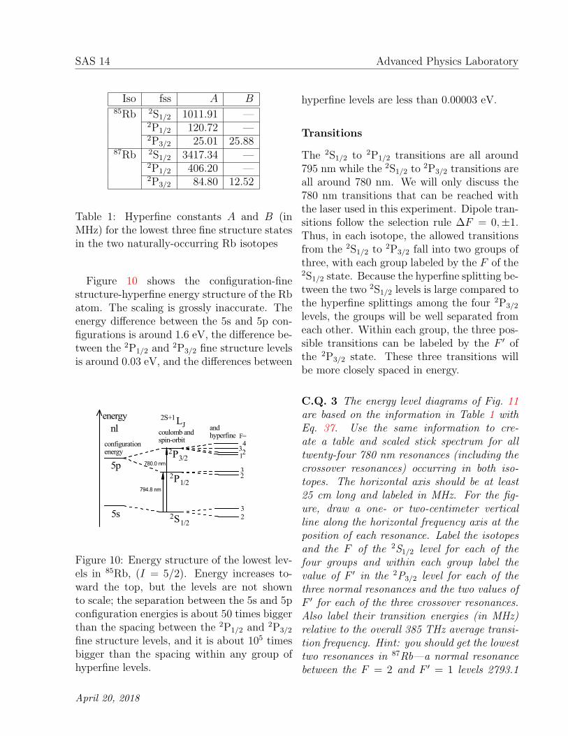
Iso fss A B85Rb 2S1/2 1011.91 —

2P1/2 120.72 —2P3/2 25.01 25.88

87Rb 2S1/2 3417.34 —2P1/2 406.20 —2P3/2 84.80 12.52

Table 1: Hyperfine constants A and B (inMHz) for the lowest three fine structure statesin the two naturally-occurring Rb isotopes

Figure 10 shows the configuration-finestructure-hyperfine energy structure of the Rbatom. The scaling is grossly inaccurate. Theenergy difference between the 5s and 5p con-figurations is around 1.6 eV, the difference be-tween the 2P1/2 and

2P3/2 fine structure levelsis around 0.03 eV, and the differences between

5s

5p

2S1/2

2P1/2

2P3/2

configurationenergy

coulomb andspin-orbit

andhyperfine F=

12

34

32

3

2

nl

2S+1LJenergy

794.8 nm

780.0 nm

Figure 10: Energy structure of the lowest lev-els in 85Rb, (I = 5/2). Energy increases to-ward the top, but the levels are not shownto scale; the separation between the 5s and 5pconfiguration energies is about 50 times biggerthan the spacing between the 2P1/2 and 2P3/2

fine structure levels, and it is about 105 timesbigger than the spacing within any group ofhyperfine levels.

hyperfine levels are less than 0.00003 eV.

Transitions

The 2S1/2 to 2P1/2 transitions are all around795 nm while the 2S1/2 to

2P3/2 transitions areall around 780 nm. We will only discuss the780 nm transitions that can be reached withthe laser used in this experiment. Dipole tran-sitions follow the selection rule ∆F = 0,±1.Thus, in each isotope, the allowed transitionsfrom the 2S1/2 to 2P3/2 fall into two groups ofthree, with each group labeled by the F of the2S1/2 state. Because the hyperfine splitting be-tween the two 2S1/2 levels is large compared tothe hyperfine splittings among the four 2P3/2

levels, the groups will be well separated fromeach other. Within each group, the three pos-sible transitions can be labeled by the F ′ ofthe 2P3/2 state. These three transitions willbe more closely spaced in energy.

C.Q. 3 The energy level diagrams of Fig. 11are based on the information in Table 1 withEq. 37. Use the same information to cre-ate a table and scaled stick spectrum for alltwenty-four 780 nm resonances (including thecrossover resonances) occurring in both iso-topes. The horizontal axis should be at least25 cm long and labeled in MHz. For the fig-ure, draw a one- or two-centimeter verticalline along the horizontal frequency axis at theposition of each resonance. Label the isotopesand the F of the 2S1/2 level for each of thefour groups and within each group label thevalue of F ′ in the 2P3/2 level for each of thethree normal resonances and the two values ofF ′ for each of the three crossover resonances.Also label their transition energies (in MHz)relative to the overall 385 THz average transi-tion frequency. Hint: you should get the lowesttwo resonances in 87Rb—a normal resonancebetween the F = 2 and F ′ = 1 levels 2793.1

April 20, 2018

Saturated Absorption Spectroscopy SAS 15

Figure 11: Energy levels for 85Rb and 87Rb (not to scale). Note that the hyperfine splittingsare about an order of magnitude larger in the ground 2S1/2 levels compared to the excited2P3/2 levels.

MHz below the average and a crossover reso-nance between the F = 2 and F ′ = 1, 2 levels2714.5 MHz below the average. The highestenergy resonance is again in 87Rb; a normalresonance from F = 1 to F ′ = 2 4198.7 MHzabove the average.

Apparatus

Laser Safety

The diode laser used in this experiment hassufficient intensity to permanently damageyour eye. In addition, its wavelength (around780 nm) is nearly invisible. Safety gogglesmust be worn when working on this ex-periment. You should also follow standardlaser safety procedures as well.

1. Remove all reflective objects from yourperson (e.g., watches, shiny jewelry).

2. Make sure that you block all stray reflec-tions coming from your experiment.

3. Never be at eye level with the laserbeam (e.g., by leaning down).

4. Take care when changing optics in yourexperiment so as not to inadvertentlyplace a highly reflective object (glass, mir-ror, post) into the beam.

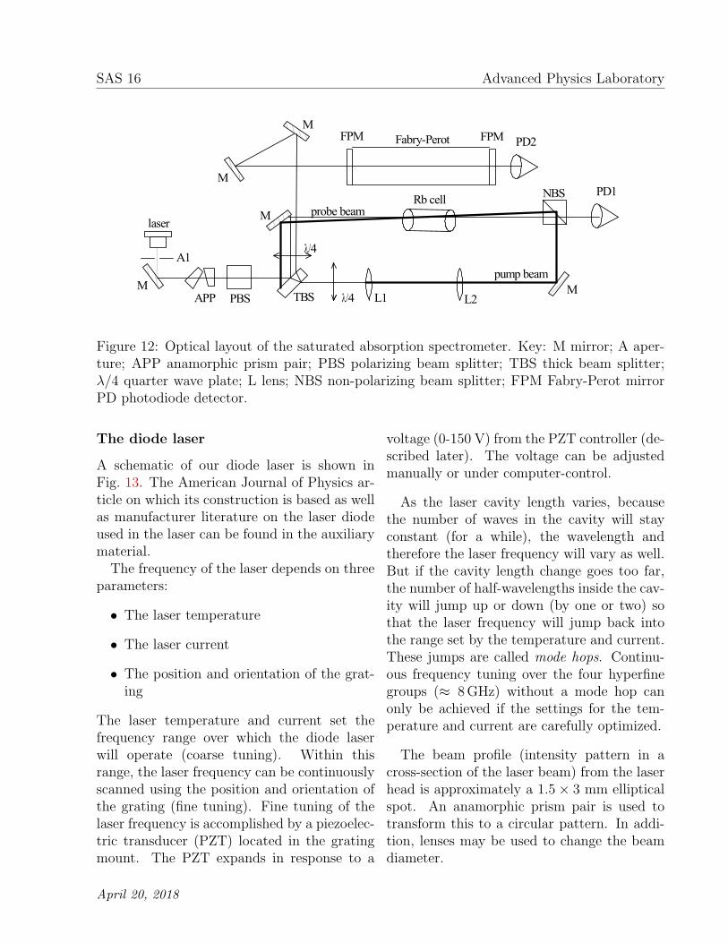
The layout of the saturated absorption spec-trometer is shown in Fig. 12. Two weak beamsare reflected off the front and rear surfaces of athick beam splitter (about 4% each). One (theprobe beam) is directed through the rubidiumcell from left to right and then onto a photo-diode detector. The other is directed througha Fabry-Perot interferometer and onto a sec-ond photodiode detector for calibrating thefrequency scan.The strong beam is transmitted through the

thick beam splitter. The two lenses after thebeam splitter should be left out at first andonly used if needed to expand the laser beam.This is the pump beam passing through thecell from right to left, overlapping the probebeam and propagating in the opposite direc-tion. (The intersection angle is exaggerated inthe figure.)You should not adjust the components from

the thick beam splitter back to the laser.

April 20, 2018

SAS 16 Advanced Physics Laboratory

laser

TBS

PD2Fabry-Perot

Rb cell

pump beam

probe beam

A1

APP PBS λ/4 L2L1

λ/4

M

M

PD1NBS

M

M

M

FPM FPM

Figure 12: Optical layout of the saturated absorption spectrometer. Key: M mirror; A aper-ture; APP anamorphic prism pair; PBS polarizing beam splitter; TBS thick beam splitter;λ/4 quarter wave plate; L lens; NBS non-polarizing beam splitter; FPM Fabry-Perot mirrorPD photodiode detector.

The diode laser

A schematic of our diode laser is shown inFig. 13. The American Journal of Physics ar-ticle on which its construction is based as wellas manufacturer literature on the laser diodeused in the laser can be found in the auxiliarymaterial.The frequency of the laser depends on three

parameters:

• The laser temperature

• The laser current

• The position and orientation of the grat-ing

The laser temperature and current set thefrequency range over which the diode laserwill operate (coarse tuning). Within thisrange, the laser frequency can be continuouslyscanned using the position and orientation ofthe grating (fine tuning). Fine tuning of thelaser frequency is accomplished by a piezoelec-tric transducer (PZT) located in the gratingmount. The PZT expands in response to a

voltage (0-150 V) from the PZT controller (de-scribed later). The voltage can be adjustedmanually or under computer-control.

As the laser cavity length varies, becausethe number of waves in the cavity will stayconstant (for a while), the wavelength andtherefore the laser frequency will vary as well.But if the cavity length change goes too far,the number of half-wavelengths inside the cav-ity will jump up or down (by one or two) sothat the laser frequency will jump back intothe range set by the temperature and current.These jumps are called mode hops. Continu-ous frequency tuning over the four hyperfinegroups (≈ 8GHz) without a mode hop canonly be achieved if the settings for the tem-perature and current are carefully optimized.

The beam profile (intensity pattern in across-section of the laser beam) from the laserhead is approximately a 1.5× 3 mm ellipticalspot. An anamorphic prism pair is used totransform this to a circular pattern. In addi-tion, lenses may be used to change the beamdiameter.

April 20, 2018

Saturated Absorption Spectroscopy SAS 17

ODVHUGLRGH

YHUWWLOW

FRDUVHIUHT

JUDWLQJ

OHQV

EHDP

HQFORVXUH

3=7

IRFXV

7

7

EDVHSODWH

Figure 13: Schematic of our diode laser. Ex-cept for the thermistors (T), the temperaturecontrol elements and electrical connections arenot shown.

Beam Paths

Several beams are created from the singlebeam coming from the laser. The polarizingbeam splitter and the quarter-wave plate helpprevent the pump beam from feeding back intothe laser cavity thereby affecting the laser out-put.

The thick beam splitter creates the threebeams used in the experiment. Two beams—one reflected off the front surface and one re-flected off the back surface—create the probebeam and the beam sent through the Fabry-Perot interferometer. Each of these beamscontains about 4% of the laser output. About92% passes through this beam splitter to be-come the pump beam.

You should also check for additional beams,

particularly from the polarizing and non-polarizing beam splitters, and use beam blocksfor any that are directed toward areas wherepeople have access.

Photodetectors

Two photodetectors are used to monitor thelaser beam intensities. A bias voltage from abattery (≈ 22 V) is applied to the photode-tector which then acts as a current source.The current is proportional to the laser powerimpinging on the detector and is converted toa voltage (for measurement) either by send-ing it through a low noise current amplifier orby letting it flow through a resistor to ground.With the latter method, the voltage developedacross the resistor subtracts from the batteryvoltage and the resistance should be adjustedto keep it below one volt.

Fabry-Perot Interferometer

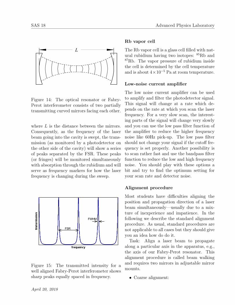
Once the laser temperature has stabilized anda laser current has been set, a voltage rampwill be applied to the PZT causing the laserfrequency to smoothly sweep over several res-onance frequencies of the rubidium atoms inthe cell. The laser frequency during the sweepis monitored using a confocal Fabry-Perot in-terferometer. The Fabry-Perot consists of twopartially transmitting, identically-curved mir-rors separated by their radius of curvature asshown in Fig. 14.

With the laser well aligned going into theFabry-Perot cavity, Fig. 15 shows how muchis transmitted through the cavity as a func-tion of the laser frequency. The Fabry-Perotonly transmits the laser beam at a set of dis-crete frequencies separated by the free spectralrange (FSR). For a confocal Fabry-Perot it isgiven by:

FSR =c

4L(38)

April 20, 2018

SAS 18 Advanced Physics Laboratory

L

Figure 14: The optical resonator or Fabry-Perot interferometer consists of two partiallytransmitting curved mirrors facing each other.

where L is the distance between the mirrors.Consequently, as the frequency of the laserbeam going into the cavity is swept, the trans-mission (as monitored by a photodetector onthe other side of the cavity) will show a seriesof peaks separated by the FSR. These peaks(or fringes) will be monitored simultaneouslywith absorption through the rubidium and willserve as frequency markers for how the laserfrequency is changing during the sweep.

FSR

FWHM

Figure 15: The transmitted intensity for awell aligned Fabry-Perot interferometer showssharp peaks equally spaced in frequency.

Rb vapor cell

The Rb vapor cell is a glass cell filled with nat-ural rubidium having two isotopes: 85Rb and87Rb. The vapor pressure of rubidium insidethe cell is determined by the cell temperatureand is about 4×10−5 Pa at room temperature.

Low-noise current amplifier

The low noise current amplifier can be usedto amplify and filter the photodetector signal.This signal will change at a rate which de-pends on the rate at which you scan the laserfrequency. For a very slow scan, the interest-ing parts of the signal will change very slowlyand you can use the low pass filter function ofthe amplifier to reduce the higher frequencynoise like 60Hz pick-up. The low pass filtershould not change your signal if the cutoff fre-quency is set properly. Another possibility isto scan rather fast and use the bandpass filterfunction to reduce the low and high frequencynoise. You should play with these options abit and try to find the optimum setting foryour scan rate and detector noise.

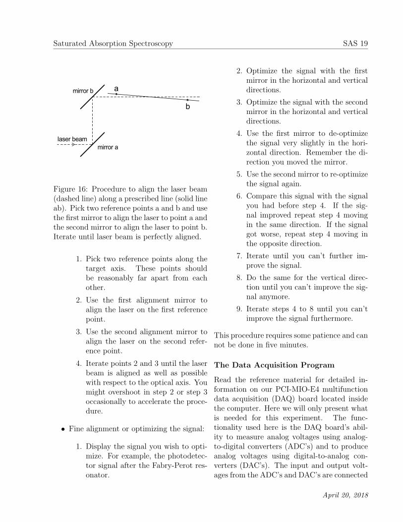
Alignment procedure

Most students have difficulties aligning theposition and propagation direction of a laserbeam simultaneously—usually due to a mix-ture of inexperience and impatience. In thefollowing we describe the standard alignmentprocedure. As usual, standard procedures arenot applicable to all cases but they should giveyou an idea how do do it.Task: Align a laser beam to propagate

along a particular axis in the apparatus, e.g.,the axis of our Fabry-Perot resonator. Thisalignment procedure is called beam walkingand requires two mirrors in adjustable mirrormounts.

• Coarse alignment:

April 20, 2018

Saturated Absorption Spectroscopy SAS 19

a

b

mirror a

mirror b

laser beam

Figure 16: Procedure to align the laser beam(dashed line) along a prescribed line (solid lineab). Pick two reference points a and b and usethe first mirror to align the laser to point a andthe second mirror to align the laser to point b.Iterate until laser beam is perfectly aligned.

1. Pick two reference points along thetarget axis. These points shouldbe reasonably far apart from eachother.

2. Use the first alignment mirror toalign the laser on the first referencepoint.

3. Use the second alignment mirror toalign the laser on the second refer-ence point.

4. Iterate points 2 and 3 until the laserbeam is aligned as well as possiblewith respect to the optical axis. Youmight overshoot in step 2 or step 3occasionally to accelerate the proce-dure.

• Fine alignment or optimizing the signal:

1. Display the signal you wish to opti-mize. For example, the photodetec-tor signal after the Fabry-Perot res-onator.

2. Optimize the signal with the firstmirror in the horizontal and verticaldirections.

3. Optimize the signal with the secondmirror in the horizontal and verticaldirections.

4. Use the first mirror to de-optimizethe signal very slightly in the hori-zontal direction. Remember the di-rection you moved the mirror.

5. Use the second mirror to re-optimizethe signal again.

6. Compare this signal with the signalyou had before step 4. If the sig-nal improved repeat step 4 movingin the same direction. If the signalgot worse, repeat step 4 moving inthe opposite direction.

7. Iterate until you can’t further im-prove the signal.

8. Do the same for the vertical direc-tion until you can’t improve the sig-nal anymore.

9. Iterate steps 4 to 8 until you can’timprove the signal furthermore.

This procedure requires some patience and cannot be done in five minutes.

The Data Acquisition Program

Read the reference material for detailed in-formation on our PCI-MIO-E4 multifunctiondata acquisition (DAQ) board located insidethe computer. Here we will only present whatis needed for this experiment. The func-tionality used here is the DAQ board’s abil-ity to measure analog voltages using analog-to-digital converters (ADC’s) and to produceanalog voltages using digital-to-analog con-verters (DAC’s). The input and output volt-ages from the ADC’s and DAC’s are connected

April 20, 2018

SAS 20 Advanced Physics Laboratory

to and from the experiment through the BNC-2090 interface box.The DAQ board will be programmed to gen-

erate a (discrete) voltage sweep which is sentto the PZT controller to sweep the laser fre-quency. While the voltage sweep is occurring,the DAQ board is programmed to simultane-ously read any photodetectors monitoring theprobe, pump, and/or the Fabry-Perot laserbeam intensities.There are two, 12-bit DAC’s (DAC0 and

DAC1) on our DAQ board and both are usedto generate the sweep. They are set to run inunipolar mode so that when they are sent inte-gers N from 0 to 4095, they produce propor-tional voltages vout from 0 to some referencevoltage vref.

vout = vrefN

4095(39)

The voltages appear at the DAC0OUT andDAC1OUT outputs on the DAQ interface box.The reference voltage vref for either DAC canbe chosen to be an on-board 10 V source orany value from 0 to 11 V as applied to theEXTREF input on the DAQ interface box.Our data acquisition program runs DAC1 in

the 10 V internal reference mode to create afixed voltage at DAC1OUT, which is then con-nected to the EXTREF input and becomes thevoltage reference vref for DAC0. The DAC0programming integers are a repeating triangu-lar ramp starting N=0, 1, 2 ..., Nmax and thengoing backward from Nmax back to 0 (whereNmax is chosen by the user). This program-ming thereby generates a triangular voltagewaveform from zero to vmax and then back tozero, where

vmax = vrefNmax

4095(40)

The properties of the triangle ramp arespecified on the program’s front panel settings

for the DAC1 voltage (vref) (labeled ramp ref(V)) and the value of Nmax (labeled ramp size).The speed of the sweep is determined by thefront panel setting of the sampling rate control.It is specified in samples per second and givesthe rate at which the DAC0 output changesduring a sweep. Thus, for example, with theramp size set for 2048, the DAC1OUT set for4 V, and the Sweep rate set for 10000/s, theramp will take about 204.8 ms to go from 0to 2 V (2048 · 4V/4096) and another 204.8 msto come back down to zero, after which it re-peats.

The triangle ramp should be connected toEXT INPUT on the MDT691 Piezo Driver.This module amplifies the ramp by a factor of15 and adds an offset controlled by an OUT-PUT ADJ knob on the front of the module toproduce the actual voltage ramp at its OUT-PUT. This output drives the PZT in the laserhead which in turn changes the laser cavitylength and thus the laser frequency. To changethe starting point of the ramp sent to the PZTin the laser head, you should simply offset itusing the OUTPUT ADJ knob. Alternatively,the front panel control ramp start can be setat a non-zero value to have the DAC0 pro-gramming integers begin at that value. Forexample, setting the ramp start to 1024 andthe ramp size to 2048 makes the programmingintegers sent to DAC0 to run from 1024 to3072 (and back down again). Then, for exam-ple, if vref were set for 8 V, the ramp would gofrom 2 V to 6 V.

Voltages from the photodetector outputsshould be connected to any of the inputs tothe analog-to-digital converter (ADC) on theinterface box. These inputs are connected toa multiplexer, which is a fast, computer con-trolled switch to select which input is passedon to be measured by the ADC. Before be-ing measured by the ADC, the signal is ampli-fied by a programmable gain amplifier (PGA).

April 20, 2018

Saturated Absorption Spectroscopy SAS 21

The gain of this amplifier and the configura-tion (unipolar or bipolar) is determined by theRange control on the front panel. You shouldgenerally use the most sensitive range possiblefor the signal you wish to measure so that the12-bit precision of the ADC is most fully uti-lized. When measuring more than one analoginput, it is also preferable if they all use thesame range so that the PGA does not have tochange settings as it reads each input.

Measurements

Turning the Diode Laser On and Off

1. Ask the instructor to show you how toturn on the laser electronics. The LFI-3526 temperature controller will maintainthe aluminum baseplate at a temperatureabout 10 degrees below room temperatureusing a thermoelectric cooler. The home-made interface box (with a white panelon the front and a power switch on theback) contains a second temperature con-trol stage which heats the diode mount-ing block about 2 degrees with a resis-tive heater. Check that the fan under thelaser head comes on and is suitably po-sitioned to blow on the laser head heatsink. Watch out that you don’t skin yourfingers moving the fan as the blade is un-shielded. The fan sits on a thin foam baseto minimize vibrations.

2. Do not change the temperature controllerset point, but learn how to read it andwrite its present value in your lab note-book. The setting is the voltage acrossa 10 kΩ thermistor mounted to the laserhead’s aluminum baseplate and used forfeedback to stabilize the temperature. Itshould be set to produce the correct tem-perature to allow the laser to operate ata wavelength of 780 nm. The laser fre-

quency depends strongly on temperatureso wait for the temperature to stabilizebefore making other adjustments.

3. Check that the laser beam paths are allclear of reflective objects.

4. Turn on the LFI-4505 laser diode currentcontroller. When you push the OUTPUTON button, the laser current comes onand the diode laser starts lasing. Thelaser current needed is typically some-where in the range from 60-90 mA. Fornow, look at the laser output beam withan infrared viewing card and watch thelaser beam come on as you increase thelaser current past the 40 mA or so thresh-old current needed for lasing. Watch thebeam intensify as you bring the currentup to around 70 mA.

5. Later, when you need to turn the laseroff, first turn down the laser current tozero, then hit the OUTPUT ON buttonagain, then push the power button. Af-ter the laser is powered off, the rest ofthe laser electronics can turned off by theswitch on the outlet box. The computerand detector electronics should be pow-ered from another outlet box and shouldbe turned off separately. Also rememberto turn off the battery-powered photodi-ode detectors.

Tuning the laser

6. Align the beam through the center of theF-P and onto its detector. Align theprobe beam through the center of the Rbcell and onto its detector. Align the pumpbeam to be collinear with the probe beambut propagating in the opposite direction.Turn on the detectors and the PAR cur-rent preamp.

April 20, 2018

SAS 22 Advanced Physics Laboratory

(a) (b)

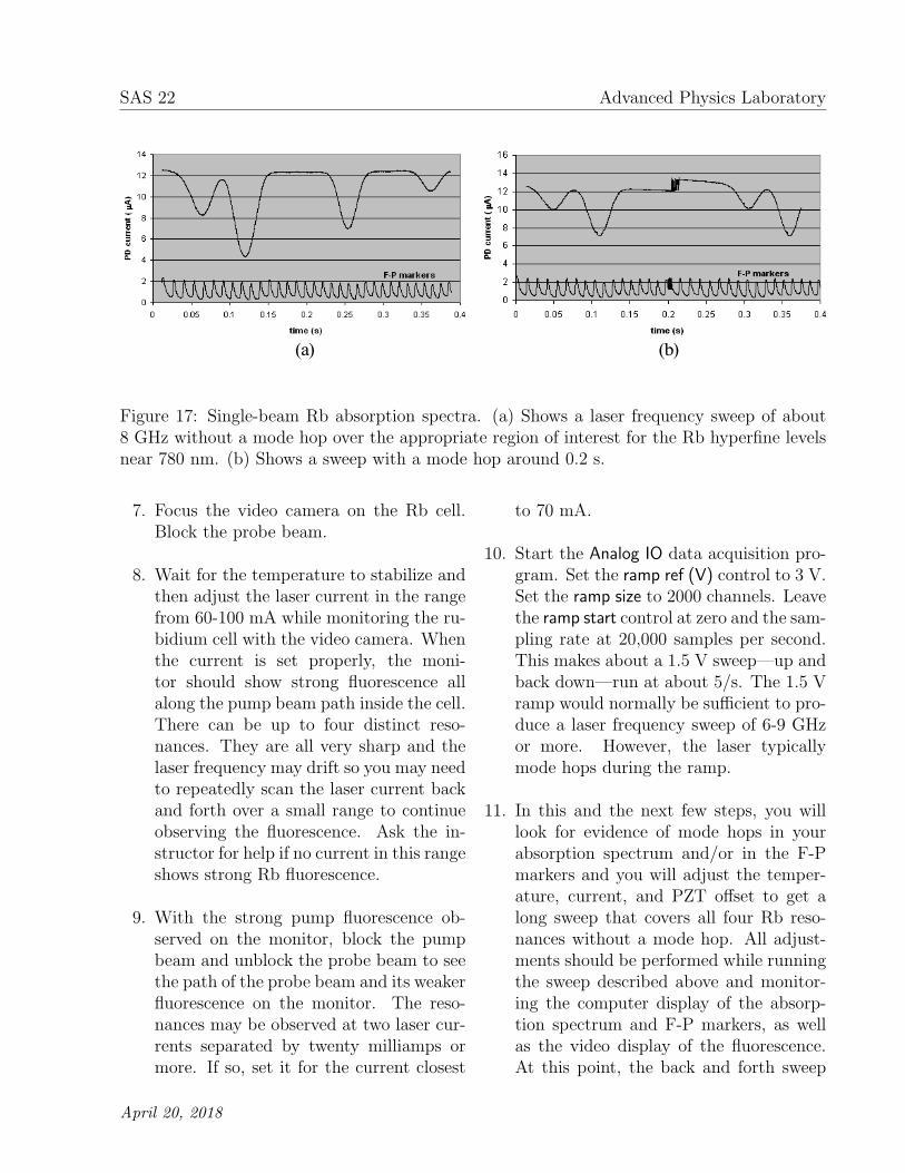
Figure 17: Single-beam Rb absorption spectra. (a) Shows a laser frequency sweep of about8 GHz without a mode hop over the appropriate region of interest for the Rb hyperfine levelsnear 780 nm. (b) Shows a sweep with a mode hop around 0.2 s.

7. Focus the video camera on the Rb cell.Block the probe beam.

8. Wait for the temperature to stabilize andthen adjust the laser current in the rangefrom 60-100 mA while monitoring the ru-bidium cell with the video camera. Whenthe current is set properly, the moni-tor should show strong fluorescence allalong the pump beam path inside the cell.There can be up to four distinct reso-nances. They are all very sharp and thelaser frequency may drift so you may needto repeatedly scan the laser current backand forth over a small range to continueobserving the fluorescence. Ask the in-structor for help if no current in this rangeshows strong Rb fluorescence.

9. With the strong pump fluorescence ob-served on the monitor, block the pumpbeam and unblock the probe beam to seethe path of the probe beam and its weakerfluorescence on the monitor. The reso-nances may be observed at two laser cur-rents separated by twenty milliamps ormore. If so, set it for the current closest

to 70 mA.

10. Start the Analog IO data acquisition pro-gram. Set the ramp ref (V) control to 3 V.Set the ramp size to 2000 channels. Leavethe ramp start control at zero and the sam-pling rate at 20,000 samples per second.This makes about a 1.5 V sweep—up andback down—run at about 5/s. The 1.5 Vramp would normally be sufficient to pro-duce a laser frequency sweep of 6-9 GHzor more. However, the laser typicallymode hops during the ramp.

11. In this and the next few steps, you willlook for evidence of mode hops in yourabsorption spectrum and/or in the F-Pmarkers and you will adjust the temper-ature, current, and PZT offset to get along sweep that covers all four Rb reso-nances without a mode hop. All adjust-ments should be performed while runningthe sweep described above and monitor-ing the computer display of the absorp-tion spectrum and F-P markers, as wellas the video display of the fluorescence.At this point, the back and forth sweep

April 20, 2018

Saturated Absorption Spectroscopy SAS 23

should produce a blinking fluorescence onthe camera video. Turn off all preampfiltering. You may need to adjust thegain settings on the DAQ board’s ADCso that the measured signals are not satu-rating the ADC. Try to adjust the currentpreamplifier gain so that the absorptionspectrum has just under 0.5 V baseline(the signal level away from the peaks) andthen be sure to adjust the ADC gain for0-0.5V signals. Also adjust the F-P detec-tor resistor so that the F-P peaks are alsojust under a 0.5 V and adjust the ADCgain for 0-0.5 V signals.

12. A good absorption spectrum with F-Pmarkers (for only the half-sweep up ofthe up and down triangular waveform) isshown in Fig. 17(a). Fig. 17(b) showswhat these two signals look like with asingle mode hop about halfway into thesweep. Notice the break in the F-P mark-ers and how the section of the absorptionspectrum repeats after the 0.2 s mark asthe laser frequency continues scanning af-ter the abrupt change in frequency causedby the mode hop. Even without any Rbabsorption, the lasers intensity may notbe very constant over the entire sweep.If this is the case, the photodetector cur-rent between absorption peaks from oneside of the sweep to the other will showa significant slope. This is partly becausethe beam from the laser changes directiona small amount as the piezo scans and thebeam may then move partially on and offthe detector by a small amount. However,if the detected laser intensity varies morethan about 10%, the beam may be hittingvery near the edge of the detector or oneof the mirrors or beam splitters therebymaking the effect bigger than it could be.Fix this problem if it occurs by better cen-

tering the beam on the detectors, mirrors,or splitters.

13. Adjust the PZT offset knob to get thelongest possible sweep without a modehop while also trying to cover the fre-quency range for the four absorptionpeaks. Adjust the laser current 1 or 2 mAone way or the other and then go back tothe PZT knob to see if the sweep is im-proving in length or frequency coverage.Repeat until you have a feel for how thisworks and have roughly found the bestpossible sweep.

14. If no combination of laser current andPZT offset gives a frequency sweep thatshows all four Rb hyperfine groups, thelaser temperature will need to be ad-justed. Save the best spectrum you cur-rently have for later comparisons. Thetemperature should be changed in smallsteps corresponding to about 0.05-0.10 kΩon the 10 kΩ thermistor used to control it.Start by increasing the setting by 0.05 kΩ(lowering the temperature). After chang-ing it, go back to the previous step. Ifthe frequency sweep improved, but is stillnot long enough, change the tempera-ture controller by another 0.05 kΩ in thesame direction. Otherwise, change it inthe opposite direction. Continue iterat-ing these two steps until you have the de-sired sweep. Ask the instructor for help ifthis step is taking more than 60 minutesor if the temperature controller has beenchanged by 0.25 kΩ without getting theneeded sweep. Keep in mind, however,that on some days it seems the best thelaser can do is a sweep that only coversthree out of the four peaks. In this case,the four peaks can usually be observedthree at a time in two separate sweepswith slightly different settings on the PZT

April 20, 2018

SAS 24 Advanced Physics Laboratory

or laser current controller.

Preliminary Measurements

15. Measure the width (FWHM) and spac-ing between the F-P fringe peaks and de-termine the finesse, which is the ratio ofthe spacing to the FWHM. If the finesseis below three, you may want to adjustthe beam steering to better align it tothe Fabry-Perot. Note the spacing be-tween the fringes. Measure the F-P mir-ror spacing and calculate the free spectralrange. Measure the distance (in channels)between the F-P frequency markers atvarious places within the sweep and notethe nonlinearity of the sweep. The non-linearity will complicate the analysis be-cause the frequency spacing between datapoints will not be constant.

16. Change the sweep to 4000 points withvref = 1.5 V to produce about the samesize sweep and explain how the F-P peaksare affected. make sure all absorptionspectra have the F-P frequency markersalong with them. They will be needed toconvert the spacing between Rb absorp-tion features (such as peak positions andwidths) to frequency units.

There are several ways the F-P markers canbe used to perform the conversion. The ab-sorption spectra are normally plotted vs. timeor channel number. In one method, the lo-cation of the F-P markers in time or chan-nels would be determined using cursors. Thensince the spacing between frequency markersis constant and is given by the FSR (let’s callit ∆ν), the frequency at consecutive markerswould be taken as ν0, ν0+∆ν, ν0+2∆ν, ... Thefrequency ν0 is about 3.85 × 1014 Hz and notreally determined with our apparatus. How-ever, we will only be interested in frequency

differences so this is not a problem. Thenthe frequency at the markers can be fit to aquadratic or cubic polynomial in the time orchannel number where the F-P peak occurredand the polynomial coefficients can then beused to convert the time or channel number ofspectral features to frequency units.A second, slightly simpler technique would

be to count whole marker spacings betweenfeatures and interpolate the location of fea-tures as fractions of the spacing relative to themarkers located near them. The whole andfractional parts multiplied by the FSR wouldthen give the frequency spacing between thefeatures.

Doppler broadening and Laser Absorp-tion

17. Obtain a spectrum of the four absorptiongroups (with the F-P frequency markers)and determine the spacing of the peaksin frequency. Use this information withyour stick spectrum to identify the fourgroups. Does the frequency increase ordecrease as the PZT ramp voltage goesup?

18. For each group, measure the Doppler-broadened FWHM and compare with pre-dictions. Do you see any effects in theFWHM due to the fact that each groupincludes three transitions at different fre-quencies?

19. Measure the absorption as a function ofincident laser intensity for at least oneof the four Doppler-broadened groups.That is, use one graph cursor to mea-sure the probe detector voltage (and con-vert to a current using the preamp gain)at maximum absorption. This readingwould correspond to the transmitted in-tensity at resonance. Set the other cur-

April 20, 2018

Saturated Absorption Spectroscopy SAS 25

sor to“eyeball” a background reading atthe same place—what the voltage read-ing would be if the absorption peak werenot there. This reading, again convertedto a photocurrent) would correspond tothe incident intensity.

So that you can get the highest laserpower, move the Rb cell into the pumpbeam and move the detector behind thecell so it will measure the pump beam ab-sorption. Do not change the laser path;only adjust the Rb cell and photodetectorpositions.

Use neutral density filters to lower the in-tensity of the beam.

Be sure to keep track of the gain settingon the current preamp so that you will beable to convert the photodetector voltages tophotocurrents. Also be sure to check thebackground photocurrent, i.e., with the laserblocked, and subtract this from any photocur-rents measured with the laser on. This back-ground subtraction is particularly importantat low laser power where the background pho-tocurrent can be a sizable fraction of the total.In the following discussion, photocurrent willrefer to background corrected photocurrent.The photocurrent is proportional to the

power incident on the detector and for theThorlabs DET110 detector, the responsivity(conversion factor from incident laser powerto current) is around 0.5 A/W at 780 nm.You can also use the Industrial Fiber OpticsPhotometer at a few of the laser intensitiesfor comparison purposes. It reads directly inwatts, but is calibrated for a HeNe laser. Thereading needs to be scaled down by a factorof about 0.8 for the 780 nm light used here.To get intensity, you will also have to esti-mate the laser beam diameter and determinehow well you are hitting the detector. If thebeam is smaller than the detector, the area to

use is the beam area. If the beam is largerthan the detector, then the detector area (13mm2 for the DET110) should be used. Keepin mind that the beam probably has a roughlycircular intensity profile with the central areafairly uniform and containing around 90% ofthe power. The diameter of this central area isprobably around 1/2 to 1/3 that of the beamas measured on the IR viewing card.Make sure to get to low enough laser inten-

sities that you see the fractional transmissionbecome constant (Beer’s law region). Plot thedata in such a way that you can determinewhere the Beer’s law region ends and the frac-tional absorption starts to decrease. This hap-pens near Isat, so see if you can use your datato get a rough estimate of this quantity.Plot your data in such a way that it shows

the prediction for the absorption or transmis-sion for the strong-field case. There are severalways to do this. Explain your plot and how itdemonstrates the prediction.

C.Q. 4 Use the measured weak-field trans-mission fraction and Beer’s law (Eq. 26) withthe cell length to determine κ0. Use this κ0

with Eq. 18 to determine α0 and then use Eq. 5to determine Isat. Compare this Isat with therough value determined by the graph—whereBeer’s law starts to be violated and with theapproximate value of 1.6 mW/cm2 given in thetext.

Rb spectra

20. Return the Rb cell to its position in theprobe beam. Remove the mirror and re-place it with the beam splitter. Move thephotodetector back to its original posi-tion monitoring the probe beam absorp-tion. If necessary, realign the probe beamthrough the splitter and onto the pho-todetector. Realign the pump beam to becollinear with the probe beam. Observe

April 20, 2018

SAS 26 Advanced Physics Laboratory

the saturated absorption dips from theprobe beam. Readjust the pump beamoverlap to maximize the depth of the dips.Note how the dips disappear when youblock the pump beam. Measure the sat-urated absorption dips for each of thefour hyperfine groups and explain your re-sults. Use short sweeps that cover onlyone group at a time. Experiment withthe sweep speed, the number of points inthe sweep and the preamp gain and fil-ter settings to see how they affect yourmeasurements.

21. Measure the FWHM of one or more dipsas a function of the pump and probebeam intensities and explain your results.How do you get the narrowest resonances?Why can’t you get a FWHM as low asthe predicted natural resonance widthof 6 MHz? Hints: Is the laser trulymonochromatic?

22. If the displayed spectrum is just aboutperfectly stable from sweep to sweep, youmight try turning on the program’s aver-aging feature to improve the quality of thespectra. However, if the spectrum movesaround on the display—even a little—averaging will blur the spectrum and de-crease its quality.

23. Measure the relative splittings withineach group and use these results to iden-tify the direct and crossover resonances.

CHECKPOINT: You should have obtainedthe “no pump” spectrum (Doppler-broadenedwithout saturated absorption dips) and thesaturated absorption spectrum (with thepump beam and showing the saturated ab-sorption dips). Both spectra should cover atleast three of the four possible groups of hyper-fine transitions (with the same lower 2S1/2 hy-

perfine level) and they should include the over-layed Fabry-Perot peaks. The Fabry-Perotmirror spacing should be measured and usedto determine the free spectral range, whichshould be used with the overlayed fringesto determine (in MHz) the following spec-tral features: (a) The separation between theDoppler-broadened peaks from the same iso-tope of the “no pump” spectrum. Comparewith expectations based on the energy level di-agrams in Fig. 11. (b) The FWHM of the eachDoppler-broadened peak. Compare with thepredictions based on Eq. 17. (c) The FWHMof the narrowest saturated absorption dip.

April 20, 2018