- - -

,.._ ... N A S A TECHNICAL NOTE N A S A T N D-3004-

C. I

A N A

KI R I I

SATISFACTION OF ASYMPTOTIC BOUNDARY CONDITIONS IN NUMERICAL SOLUTION OF SYSTEMS OF NONLINEAR EQUATIONS OF BOUNDARY-LAYER TYPE

' by Philip R. Nuchtsheim und PunZ Swigert

J Lewis R eseurch Center Clevelund, Ohio

N A T I O N A L AERONAUTICS A N D SPACE A D M I N I S T R A T I O N WASHINGTO 6 5

https://ntrs.nasa.gov/search.jsp?R=19650026350 2018-06-05T20:10:30+00:00Z

TECH LIBRARY KAFB, NM

IIllilllllll111llllllllllll1llllllllIll911 0L30090

SATISFACTION OF ASYMPTOTIC BOUNDARY CONDITIONS IN

NUMERICAL SOLUTION OF SYSTEMS O F NONLINEAR

EQUATIONS O F BOUNDARY-LAYER T Y P E

By P h i l i p R. Nach t she im a n d P a u l Swiger t

L e w i s R e s e a r c h C e n t e r Cleve land , Ohio

.

NATIONAL AERONAUTICS AND SPACE ADMINISTRATION

For sale by the Clearinghouse for Federal Scientific and Technical Information Springfield, Virginia 22151 - Price 52.00

SATISFACTION OF ASYMPTOTIC BOUNDARY CONDITIONS IN NUMERICAL SOLUTION

OF SYSTEMS OF NONLINEAR EQUATIONS OF BOUNDARY-LAYER TYPE

by P h i l i p R. Nachtsheim and P a u l Swigert

Lewis Research Center

SUMMARY

A method for the numerical solution of differential equations of the boundary-layer type is presented. The asymptotic boundary conditions are satisfied at the edge of the boundary layer by adjusting the initial conditions s o that the mean square e r r o r between the computed variables and the asymptotic values is minimized. Convergence to a solu­tion is rapid and appears to be insensitive to the initial guesses of the initial conditions. Use of a least-squares convergence cri terion leads to the unique solution even in the case of retarded main s t ream flows. A description of the method is given, and two examples taken f rom boundary-layer theory are worked. For the Falkner-Skan differen­tial equation, the relation betwee.n the wedge angle and the shear s t r e s s at the wall is obtained.

INTRODUCTION

The numerical integration of the ordinary differential equations of boundary-layer theory involves the satisfaction of asymptotic boundary conditions; that is, some bound­ary conditions a r e specified at the initial point o r wall, and others are specified as limits that must be approached at large values of the independent variable corresponding to the edge of the boundary layer. In order to integrate the differential equations numerically from the wall to the edge of the boundary layer, it is necessary to specify as many addi­tional conditions at the wall as there a r e conditions to be satisfied at the edge of the boundary layer. These additional initial conditions have to be varied in order to satisfy the conditions at the edge of the boundary layer. All methods that have been used to find the proper initial conditions rely on the fact that, for large values of the independent variable, the integrals of the differential equations depend on the initial conditions. One method that has been used to find the proper initial conditions, called the initial-value method (ref. l), is that of obtaining integrals of the differential equations with guessed initial conditions; that is, an attempt is made to integrate the differential equations to

.

the edge of the boundary layer. If this can be accomplished, corrections a re made for the initial guesses by the Newton-Raphson method, and the process is repeated until con­vergence is achieved.

In order to ca r ry out this iteration, additional differential equations have to be inte­grated. The additional differential equations are obtained by differentiating the t e rms of the original differential equation with respect to the initial conditions. The integrals of these additional differential equations, henceforth referred to as perturbation equations, give the rate of change of the integrals of the original differential equation with respect to the initial conditions.

Another method that has been used, called quasilinearization (ref. 2), is similar in principle to the initial-value method, except that the original differential equations a r e linearized. The resulting linear differential equations for the current approximation a r e inhomogeneous, since they also contain the previous approximation as members.

The integrals of the perturbation equations of the initial-value method correspond to a complementary solution of the linear differential equations of the quasilinearization method. In application, the two methods are different in that, in the quasilinearization method, the complementary solutions a r e used to obtain solutions to the inhomogeneous linear differential equations, whereas in the initial-value method, the integrals of the perturbation equations a r e used to adjust the starting values at the initial point. A dis­advantage associated with the quasilinearization method is that functions representing the previous approximation have to be stored in order to construct the current approximation. Furthermore, the solution of the inhomogeneous equation obtained by combining com­plementary solutions and a particular integral is usually not well determined except near the origin o r initial point, as pointed out by Hartree (ref. 3). The solutions of the per­turbation equations, however, can be used to determine the proper initial conditions closely. This is the procedure that is followed in the initial-value method.

Both methods have been used to obtain solutions of the boundary-layer equations. Neither of these methods, however, has solved the problem of when to stop the integra­tion. Since one boundary condition is specified as a limit that must be approached at large values of the independent variable, the integration should be stopped at a value of the independent variable that is sufficiently large so that the various functions a re approaching their asymptotic values. This value of the independent variable could properly be called the edge of the boundary layer. In the various methods used to solve this problem, this value of the independent variable must be guessed beforehand. If the guessed value is too small, the integrals of the differential equation may not be able to satisfy the imposed conditions; o r , there may be more than one value of an initial condi­tion that leads to integrals of the differential equations that satisfy the imposed boundary conditions.

If the guessed value is too large, it is possible that the integrals of the equations

*i

i I

7

t

2

will diverge, o r that convergence to a solution is extremely slow. Another problem that sometimes besets the numerical integration of the boundary-

layer equations is the apparent insensitivity of the integrals of the boundary-layer equa­tions to the initial conditions. This difficulty appears in the integration of the Falkner-Skan differential equation (ref. 4). All the integrals of the Falkner-Skan equation for the case of nonretarded flows in the main s t ream tend to diverge except the ones with the proper initial conditions; however, for the case of retarded flows, a solution with any

b value of the initial condition near the correct one will eventually meet the proper boundary condition at infinity. The unique solution was found by Hartree (ref. 4) for retarded flows by imposing the additional condition that the desired solution is the one that approaches the boundary condition most rapidly from below. However, this behavior of the solutions can only be learned from several trial runs.

In an effort to adapt the initial-value method to the solution of differential equations with asymptotic boundary conditions, a method was developed to eliminate the problem of when to stop the integration. This method of solution is capable of satisfying the boundary conditions at the edge of the boundary layer correctly; that is, the boundary values a re approached asymptotically. This is accomplished by choosing the additional initial conditions so that the mean square e r r o r between the computed variables and the asymptotic values is minimized. A method of solution is proposed that is based on a least-squares convergence cri terion in which the edge of the boundary layer is approached in steps. The convergence rate to a solution is rapid, and convergence appears to be insensitive to the initial guesses of the initial conditions. U s e of a least-squares con­vergence criterion leads to the unique solution even in the case of retarded main s t ream flows. A description of the method is given, and two examples taken from boundary-layer theory are worked. By using this method of solution it is feasible to obtain directly, for those differential equations which contain a parameter, the relation between the properties of the solutions and the values of the parameter. For the Falkner-Skan differ­ential equation, the relation between the wedge angle and the shear stress at the wall is obtained.

DESCRIPTION OF METHOD

. A description of the method can best be given by referring to a definite example of a boundary -value problem with an asymptotic boundary condition. In Falkner and Skan's treatment of the laminar boundary layer of an incompressible fluid, the following equa­tion arises (see ref. 4):

3

with the boundary conditions

(Symbols are defined in appendix A. ) Pr imes denote differentiation with respect to q, a measure of the distance from the wall. The dependent variable f is related to the usual . s t ream function. The potential flow is given by a power law. The flow velocity outside the boundary layer in the main s t ream is proportional to the distance along the wall raised to the power P / ( 2 - P) . For retarded main s t ream flow P < 0, and for non­retarded flow P -> 0.

In practice, the asymptotic boundary condition is replaced by the condition that f' = 1 to a sufficient degree of accuracy at q = q,dge, where qedge is the value of the independent variable at the edge of the boundary layer. The boundary-value problem is equivalent to the problem of finding a value of f"(0) for which the boundary condition at the edge of the boundary layer is satisfied; that is, it is desired to find a solution of the nonlinear equation

-where fkdge -- f'(qedge). The function fLdge[f"(O)] in this problem is not, in general, explicit; it will be expressed as a function of f"(0) through an integration of equation (1). With the notation x = f"(O), observe that a small change Ax in x changes f' by the amount

so that the necessary correction to a f i rs t approximation comes from the solution of the linear equation

afll = f ' + - A x ax

.I

at q = qedge'The solution of the equation for Ax can be performed provided that the partial

derivative of f ' with respect to x can be evaluated at qedge. The partial derivative can be evaluated by forming the perturbation equation for the function f'. This equation

4

4

I .~ I I­

1 ­

\.

f

-.8

1.0 2.0 3.0 4.0 5.0 Distance from wall, 7

(c) f for f '(0) - 0.85.

Figure 1. - Variation of f and f". Falkner-Skan parameter, 1.

is obtained by differentiating the t e rms in equation (1) appropriately. With the notation

the following perturbation equation is obtained:

f"'X = -(ffY + f"fx) + 2Pf'fjc

. with the initial conditions

77 = 0: fx = f 'x = 0,f"X = 1

Given an initial estimate of x = f"(O), subsequent values of x can be computed by integrating equations (1) and (2) and applying the Newton-Raphson method to obtain correc­tions.

The problem of where to stop the integration remains; that is, qedge is unknown. Figure l(a) illustrates the difficulties that arise when the boundary condition f' = 1 is

5

applied at a finite value of 7. The data for figure l(a) were obtained by integrating equation (1)for specified values of f"(0) with P = 1. The integration was stopped at q = 5. Tentative values of qedge will hereinafter be referred to as qstop. It should be noted that the problem is not that qedge is unknown, but an appropriate qStop must be determined in some fashion for use in the as yet unconverged iterations.

Figure l(a) shows f' and f" as a function of x = f"(0) at qStop = 5. It can be seen that there are two values of x that satisfy the condition f ' = 1 when qstop is taken to be 5, namely, approximately x = 0.85 and x = 1.23. Figures l(b) and (c) show * the two solutions corresponding to the two values of x. It can be concluded from this illustration that the satisfaction of the single boundary condition f' = 1 at qstop = 5 i

does not lead to a unique solution. The proper value of x can be determined by ob­serving where f" = 0. From figure l(a) it can be seen that the correct value of x is -approximately 1. 23. Satisfaction of both boundary conditions f ' = 1 and f" = 0 at

%top = 5 ensures the satisfaction of the original boundary condition of f ' , namely, that f' approaches unity asymptotically as approaches infinity. Hence, in order to satisfy the asymptotic condition at a finite value of q, the conditions f ' = 1 and f v f = 0 should both be imposed (examination of the differential equation, (eq. (l)),will reveal that all higher derivatives will be zero also); that is, Ax should be chosen so that both equations

1 = f ' + f; Ax (3)

and

are satisfied at 17 = vstop. This is, in general, impossible since there are two condi­tions and only one adjustable parameter Ax. However, a satisfactory solution that is consistent with the idea that the boundary condition cannot be satisfied exactly at a finite value of 7 is to seek the least-squares solution of equations (3) and (4)(ref. 5). Hence consider the discrepancies 6 and 62, where

6 1 = f k A X + f ' - 1

6 2 = f; Ax + f"

2 as small as possible.and attempt to find a value for Ax that will make the sum 612 + 6 2

To minimize the sum, i t is necessary to equate i ts f i rs t derivative with respect to Ax

to zero. This calculation yields a value of Ax corresponding to the minimum of the sum 2612 + 62, that is,

6

Distance from wall,

_I2 2

Figure 2. - Error as function of f"(0) for different values of TStop. Falkner-Skan param­eter, 1.

fJr(1 - f ') - fGf" A x = (5)

fJr2 + ff,' 2

Along with the discrepancies 6 and 6 consider the sum of the squares of the deviations of the computed quantities from their asymptotic values

E = (1 - f ') 2 + f" 2 (6)

Henceforth, E shall be re fer red to as the e r ror . The magnitude of E evaluated at , ?Stop gives an indication of how unsatisfactory the asymptotic boundary conditions are.

The value of x that gives Ax = 0 corresponds to the minimum with respect to -x of E, as can be seen from equation (5). In figure 2, the quantity E is shown plotted as a function of x for various values of qstop. The data for figure 2 were also obtained from the integrations that were used to prepare figure 1. It can be seen that the least-squares solution gives a unique solution for x. It is this property, that the minimum of E with respect to x, Emin, corresponds to no change in the required initial conditions, that permits the asymptotic boundary condition to be approximately satisfied at a finite value of the independent variable.

For this example, the Falkner-Skan solution with P = 1, it appears that the quantity

7

E has a definite minimum at each value of q, even at q = 0, as seen from figure 2. The edge of the boundary layer could be defined as that value of q for which the value of

Emin is less than some preassigned small value as the range of integration is increased. This gives a value of qedge-

The concept of convergence in the least-squares sense allows the initial-value method to be modified in order to solve a wide class of boundary-layer problems. To understand why the initial-value method requires modification, consider how the method can f a i l when it is applied to boundary-layer-type problems.

Recall that in the initial-value method corrections a r e obtained to the guessed initial conditions after integrating the differential equations to the edge of the boundary layer. This method can fail i f the initial guess is so poor that the integration l'blows up" (i.e . , diverges beyond a prescribed limit) before reaching the edge of the boundary layer.

This problem can be avoided and corrections to the initial conditions can be obtained by attempting to minimize the mean square e r r o r between the computed solution and the asymptotic values before reaching the edge of the boundary layer. The modification of the initial-value method consists then of finding Emin at any arbitrary value of qstop. By this modified procedure, the choice of qStop, where the minimizing process is first carried out, may be dictated by other considerations than where the edge of the boundary layer is, such as keeping the variables within prescribed limits so that the solution does not diverge. After Emin has been found, no further corrections to the initial conditions need to be made at the chosen value of qstop, and the range of integration can be in­creased if necessary.

If the value of Emin found is not small enough, it will be necessary to increase the range of integration. In this way, the edge of the boundary layer is approached in steps by successively increasing the range of integration until the correct initial conditions and the value of qedge are found. In other words, as qstop is increased, Emin tends to zero, and the required initial condition x = f"(0) also tends to a definite value. This gives the solution of the boundary-value problem.

4

e

6NUMERICAL SOLUTION

The method described in the previous section was programed in FORTRAN IV, v

double precision on the IBM 7094II-7040direct-couple system. The boundary-layer and perturbation differential equations were rewritten as systems of first-order differential equations and integrated with a predictor-corrector (Adams-Moulton) subroutine using one correction per step and a fixed increment.

The boundary-layer equations along with the perturbation equations were integrated

8

------ ------

1. 2 to the specified value of the independent vari­able. The corrections were then determined,

. 8 and the process was repeated until the relative

f change in the correction term, equation (5), was less than a small preassigned value.

. 4 Extreme accuracy was not required at the

smaller values of qStop since the boundary 0 1 2 3 4 5 conditions cannot be well satisfied there. A

Distance from wall, 7 value of 1X10m8was used at the larger values of Figure 3. - Convergence history of solution of equation (1)

qstop to check the relative change in the correcFalkner-Skan parameter, 1.

tion term. This small value seemed reasonable since convergence is so rapid.

RESULTS OF NUMERICAL SOLUTION FOR EXAMPLE 1

Figure 3 shows the solution f' of equation (1) with P = 1 as a function of the independent variable q, for the five trials needed for convergence. With an initial guess of 1.0 for f"(O), the equations were integrated to a value of qstop = 2 twice and to a value of qStop = 5 three times. Observe that, for the first integration, the values of f '

tend to deviate radically from the correct solution at a relatively small value of q. If these calculations had been carr ied out to a larger value of q, the values of f ' would have attained a magnitude so large that any use of these large numbers in a Newton-Raphson scheme would be meaningless.

TABLE I. - EFFECT OF vStop ON CONVERGENCE RATE

f"(0) (initial guess)

vstop =

f' '(0) :after two trials)

vstop= ~

f"(0)1Percent difference (after two trials)

~~

0.25 1.2799034 3.83 0.26706180 .50 1.2449846 1.00 .69205364 .75 1.2292604 -.26 .88486032 1.00 1.2266764 -.47 1.0413712 1.25 1.2266282 -.48 1.2325888 1. 50 1.2266765 -.47 1.2444813 1.75 1.2277231 -.39 1.2890732 2.00 1.2312423 -.10 1.3564389 2.25 1.2383960 .47 I. 8834930 2.50 1.2498889 1.40 2.4946776 2.75 1.2660459 2.71 ---------3.00 1.2869264 4.40 ---------

Per cent difference

-78.33 -43.85 -28.21 -15.51

.00

.96 4.58 10.04 52.80 102.39

9

1 2 3 4 5 6 7

1 2 3 4 5 6 7

TABLE II. - CONVERGENCE HISTORY O F INITIAL VALUES

(a) Example 1

%top f"(0)

2.0 1.0 2.0 1.2463981

5.0 1.2266764 5.0 1.2326729 5.0 1.2325878

1.2325878

Literature values II

Trial Correction qStop f"( 0)

2.0 1.0 .1.0 2.0 .61735605 -. 59008297 8.0 .63211384 -. 57655550

8.0 .66795925 -.52593128 8.0 .67387305 -.50916398

8.0 .67412049 -. 50790411 8.0 .67412438 -. 50789273

.67412438 -. 507892732-L - . __

gence to a solution for this example using an initial guess of f"(0) = 1, table II(a) is pre­

sented. Using quasilinearization and five corrections, Radbill (ref. 2) obtained a value of f"(0) that agrees with that of Yohner and Hansen (ref. 6) to within seven units in the third decimal place. The method developed herein reached an answer after two correc­

tions that agrees with that of Yohner and Hansen to within six units in the third decimal ?

place. After two more corrections the answer agreed to within two units in the seventh decimal place (see table II(a)). The last integration was performed as a stopping criterion for the computer. Computer time for the complete solution, using a step size of 2-4 was approximately 0.03 minute.

This example was also programmed by single precision with good results. The

10

The effect of qstop on the convergence process is illustrated in figure 2 and table I. Figure 2 shows the e r ro r , equation (6), as a function of f"(0) for different values of

%top. Observe that by initially using a small value for qstop (qStop = 2 in fig. 2) the range of meaningful initial guesses is

9increased, that is, initial guesses that yield a relatively small e r ro r . For ex­tremely large values of qstop the 4

parabola-like curves in figure 2 degenerate to a vertical line, and the initial guess is limited to the correct answer.

Table I shows the effect of qstop on the convergence rate. Also, the values of f"(0) after two trials and the percentage difference from the correct value of f"(0) for a wide range of initial guesses and two values of qstop a r e given. The conver­gence to the correct answer is always faster for the smaller qstop except when the initial guess is close to the correct answer. In fact, the two largest initial guesses "overflowed'' the computer before the larger qstop was reached. This indi­cates that a very crude initial guess may be used if the integration is carried out to a small qstop.

Ti give an idea of the rate of conver-

-

difficulty in using single precision presented itselt in the form of reducing the range of initial guesses that yielded a relatively small e r ror . Evidently, this was caused by the increased round-off e r r o r associated with the use of single precision.

Equation (1)was also integrated for the case of a retarded main s t ream flow with /3 = -0.1. However, no additional conditions such as those used by Hartree (ref. 4) had to be imposed in order to obtain the unique solution. The value of f"(O), which was obtained by minimizing the mean square e r ro r , agreed with the value obtained by Smith (ref. 7) for this case to six decimal places. A description of the flow chart and the FORTRAN

t

listing for this program are presented in appendix B.

t

EXTENSION TO SYSTEMS OF EQUATIONS

The least-squares modification of the initial-value method described in the preceding section for a differential equation with a single dependent variable can easily be general­ized to systems of equations. As an example of a problem with two dependent variables, consider the boundary-value problem for the free-convection flow about a vertical plate. This example is taken from reference 8. It consists of solving the differential equations

f"' = -3ff" + 2ft2 - h (7)

with the boundary conditions

q = O : f = f ' = O , h = l

q - - w : f ' - 0 , h - 0

Again the primes denote differentiation with respect to q (a measure of the distance from the wall), and the dependent variable f is a dimensionless form of the usual s t ream function. The dependent variable h is proportional to the temperature excess of the fluid over the ambient temperature, and Pr denotes the Prandtl number.

Since there are two asymptotic boundary conditions to satisfy, two additional initial conditions at the wall will have to be adjusted; that is, values of x = f"(0) and y s h'(0)

* are sought that will satisfy simultaneously the nonlinear equations.

hedge [f"(O), h'(O)] = 0

and fkdge[f"(O), h'(O)] = 0

- -where fkdge - f'(qedge and hedge = h('rledge). The necessary first corrections to a first approximation x and y come f rom a solution of the linear equations

11

f"'

0 = f ' + f; Ax + f'Y

Ay

and

O = h + $ A x + 5 Ay at q = r ]

edge where f; = af'/ax, f'Y = af'/ay, etc. However, in order to satisfy the asymptotic boundary conditions, the preceding equations must be supplemented by

0 = f" + f z Ax + f"Y

Ay

and

0 = h' + % A x + 5 Ay

and Ax and Ay must be found such that the sum of squares of the e r r o r s in the pre­ceding four equations be a minimum. The least-squares solution for those quantities is given by the solution of the following matrix equation:

f'f; + hhx + f"f; + h'h'

f'f' + h 5 + f"f" + h'h'Y Y

The values of x and y that give Ax = Ay = 0 correspond to the minimum with respect to x and y of the quantity

E = f' 2 + h2 + f T f 2+ h' 2 (10)

The partial derivatives with respect to x and y that appear in equation (9) are ob­tained by integrating the appropriate perturbation differential equations, The perturba­tion differential equations for the x derivatives are

X = -3(fxf" + ffg) + 4f'f; - hx (11)

and

hl,' = -3Pr(fxh' + fh;) (12)

with the initial conditions

12

. I

1.6

1.2

f .8

. 4

0

h . 4

Trial I nbe ~

! f \ ..

0 1 7 8 Distance from wall, 7

Figure 4. - Convergence history of solutions of equations (7) and (8). Prandtl number, 0.733.

The perturbation differential equations for the y derivatives a r e

f"' = -3(f Y

f" + ff")Y Y

+ 4f'f'Y - 5 and

h;: = -3Pr(f Y

h' + fh')Y

with the initial conditions

Note that the equations for the y derivatives are the same as the equations for the x derivatives. The integrals of these equations will differ since the initial conditions are different.

Note also that there are as many additional systems of perturbation equations to

13

.o E>1.0 ~

~

h'

I7 -1.2 7

.2 . 4 .6 . a 1 1.2

Figure 5. - Level curves of error against f"(0) and h'(0).

Iintegrate as there a r e asymptotic boundary conditions to meet.

NUMERICAL SOLUTION OF CONVECTIVE FLOW PROBLEM FOR EXAMPLE 2

The same general procedure used in the previous example was employed to solve this example. One notable difference is that five trials were needed at the larger value

Of %top' rather than the three trials of the first example. This is probably because of the need of adjusting two initial Conditions rather than one and because an e r r o r in one initial condition leads to an e r ro r ii; vomputing the correction t e rm of the other.

The solutions of equations (7) and (8) a r e shown in figure 4 for Pr = 0. 733. Note (as in the previous example) that the functions f' and h of figure 4 diverge radically from the true solutions, for the initial guesses of trial 1.

Table II(b) (p. 10) shows the rapid rate of convergence for this more difficult ex­ample. With initial guesses of 1. 0 and -1 . 0 for f"(0) and hl(0), respectively, con­vergence is realized after two t r ia ls with qstop = 2 and five tr ials with qstop = 8. The results a r e in close agreement with the published values of Ostrach (ref. 8).

The effect of qstop on the convergence process for this example is illustrated in figures 5(a) and (b). Level curves for the e r ro r , equation (lo), are plotted in the fl'(0), h'(0) plane for qstop = 2 in figure 5(a), and for qstop = 5 in figure 5(b). As in the previous example, by using a small value for qstop, the range of initial guesses

14

that yields a relatively small e r r o r is again increased; that is, the a rea where E is less than 1is much greater in figure 5(a) than in figure 5(b). For extremely large values

(I

*

of r l s t o p 7 that i s 7 rlstop greater than 8, the area enclosed by the level curve where E is less than 1shrinks to a point, and the initial guess is limited to the correct answer.

Computer time for the second example was about 0. 10 minute with a step size of 2-4. In both examples, the convergence was made insensitive to the initial guesses by choosing a small value of qstop for the first two trials. The answer thus obtained for the initial conditions was good enough so that qstop could be increased considerably. The error t e rm may be made as small as desirable by continuous extension of the range of integration. This e r r o r t e rm may also be used as a stopping criterion for computer calculations and finding qedge automatically. A discussion of theflow chart and the FORTRAN listing for this program are given in appendix B.

SOLUTIONS OF AN EQUATION CONTAINING A PARAMETER

Very often it is desired to examine the general properties of the solutions of a differential equation containing a parameter when the parameter is varied. For example, in the case of the Falkner and Skan differential equation (eq. (l)),which contains the parameter P, it is desirable to know the variation of f"(0) with P. The physical significance of f"(0) is that it is proportional to the shear s t r e s s at the wall.

If P > 0, the flow may be regarded as that near a wedge, and the included angle of the wedge is Pn. But i f P < 0, it can only be said that it corresponds to a flow in an adverse pressure gradient (retarded main s t ream flow). It is desired to know the be­havior of the shear stress as P is varied. It is especially important to know what value of P gives f"(0) = 0, that is, the laminar separation profile. This behavior of the solu­tions can be learned by solving equation (1)for a preassigned set of values of P and determining a set of values of f"(0).

Since the modification of the initial-value method described previously allows accu­rate solutions of equation (1)to be obtained quickly and easily, it is feasible to obtain the variation of f"(0) with P by using a more economical procedure than by obtaining solu­tions for a preassigned set of values of P. This procedure is essentially the method of steepest descent, as explained. in reference 9. It consists of finding the curve of solu­tions fT1(0)against P in the P, f"(0) plane and following it. The points that lie on the curve of solutions are the values that allow equation (1)to satisfy the imposed boundary conditions.

The curve of solutions of equation (1)in the P , f"(0) plane can be considered to be given implicitly by the equation

15

where fkdge f'(qedge ). Any point P,f"(O) in the plane may be regarded as lying on a curve fkdge = constant. If p, frl(0) is an approximate solution of equation (15), the curve

fLdge = constant will be nearly parallel t o the curve of solutions fkdge = 1, and the necessary corrections to a first approximation can be found by solving the equation

together with the equation ' e

0 = -fk AP + f'P AX (17)

at q = qedge' where fb = af'/aP and fJE = af'/ax, x = f"(0). Equation (17) guarantees that the increment (AP, Ax) Will be perpendicular to the curves fkdge = constant. Succes­sive iterations lead to a point on the curve fkdge = 1. The direction of the tangent can be obtained by solving

O = f ' + f ' -dx X d P

for dx/dP and may then be used to predict further points close to the curve. The solution of the equations for (AP, Ax) (eqs. (16) and (17)) can be performed pro­

vided that the partial derivatives of f ' with respect to x and P can be evaluated at

qedge'equation (2), as explained previously. The partial derivatives for the P variation can be

The partial derivatives with respect to x can be obtained from the solution of

evaluated by forming the perturbation equation for the function f'. This equation is ob­tained by differentiating the t e rms in equation (1) appropriately with respect to p. The following perturbation equation for the P variation is obtained

fp' = -(ffY + f"fP) + ZPf'fl, + ( f t 2 - 1) (19)

with the initial conditions

Note that equation (19) is an inhomogeneous differential equation so that the homogeneous initial conditions do not necessarily yield a trivial solution.

Furthermore, note that, if the requirement of steepest descent is dropped, for

16

example, that is, the curve of solutions is approached on a line parallel to the p-axis, equation (19) alone could be used in conjunction with equation (1) without the use of equa­tion (2) to obtain the curve of solutions f o r preassigned values of x = f"(0). In this way, the value of P that gives the separation profile f"(0) = 0 can be found.

The requirement of the asymptotic approach of the solutions to the proper values is incorporated by recognizing that the curve of solutions of equation (1)can also be con­sidered to lie on the curve given implicitly by the equation

and requiring that this equation, where f:dge = f"(qedge), be satisfied as well as equa­tion (15) at 17 = qedge. In this case, if p, f"(0) is an approximate solution of equa­tion (20), the necessary corrections to a first approximation can be found by solving the equation

0 = f" + f"P AP + fg AX (21)

together with the equation

O = -f"X AP + f"P AX

at q = qedge. The direction of the tangent can be obtained by solving

for dx/dP. The required values of AP, Ax for the asymptotic approach are obtained from the least-squares solution of equations (16), (17), (21), and (22). The least-squares solution for these quantities is given by

fb(f' - 1)+ fPf" A B = ­

f ' 2 + f; 2 + fF2 + fg 2 P

and

f g f ' - 1)+ f2 f " AX = ­

2

17

20 and the least-squares solution of equations (18) and (23) gives the direc­

1.6 tion of the tangent d

d L 2

.a

The process just described was . 4 programed for solution on the com­

puter. Very few changes were needed

0 in the program used in example 1. -.4 0 . 4

Falkner-Skan parameter, 1. 2

i3 1.6 20 Appendix B gives a discussion and the

Figure 6. - Curve of solutions: FORTRAN listing of this program. The entire curve of solutions

(fig. 6), defined by 23 points over the range P = -0.1 to 2.1 , was obtained in approxi­mately 0 . 8 minute of computer time. Two values of qstop were used for this solution; they a r e 4 . 0 and 8.0. The smaller qstop was used only twice to start the solution since the predicted points on the curve of solutions, obtained from equation (26), were accu­ra te enough to integrate directly to the larger qstop. A solution was obtained in about four iterations, for each point, in this manner.

Equations (2) and ( 19) were integrated along with equation ( 1) to give the necessary t e rms for the corrections obtained from equations (24) and (25). When convergence was realized, equation (26) was applied to predict a new solution.

The value of P where f"(0) = 0 was obtained by the method of example 1 by treat­ing P as the dependent variable; that is, f"(0) was held constant, while P was allowed to vary. This is accomplished by integrating equation (19) along with equation (1) and applying the correction factor given by

f'P( 1 - f') - f'"" AB = P

f b2 + f"P 2

Note the similarity to equation (5). This method with qStop = 16 yielded an e r r o r t e rm (eq. (6)) of less than 1x10- 28 .

The numerical value of P when f''(0) = 0 is -0.198837682 and agrees with that of reference 7 to six decimal places. When the value of p presented in reference 7 was used in the program of example 1, the solution oscillated, and convergence could not be achieved. When the value presented herein was used, no such oscillation was experienced. 18

i f

CONCLU SlONS

The two main problems of integrating the boundary-layer equations, namely, approxi­mating the missing initial conditions and determining when to stop the integration in the as yet unconverged iterations, have been reduced to an automatic initial-value technique that is easily programed on high-speed computers. The technique was successfully applied t o two problems taken from boundary-layer theory and offers promise of producing equivalent results when applied to other boundary-layer problems. The method appears to be insensitive to initial guesses and converges quickly to the solution. By this method the implicit study of differential equations containing a parameter has also been reduced to an automatic technique.

Lewis Research Center, National Aeronautics and Space Administration,

Cleveland, Ohio, June 11, 1965.

19

APPENDIX A

SYMBOLS

E

f

h

Pr

X

Ax

Y

AY

P

A/3

1)

sum of squares of e r r o r s in boundary conditions

related to s t ream function

related to temperature excess of fluid over ambient temperature

Prandtl number

x = f"(0)

increment in x

y = h'(0)

increment in y

Falkner -Skan parameter

increment in /3

measure of distance from wall

Subscripts:

edge edge of boundary layer

stop tentative values of edge of boundary layer

X denotes partial differentiation with respect t o x

Y denotes partial differentiation with respect to y

P denotes partial differentiation with respect to P

Super script:

r denotes differentiation with respect

to 11

20

I

APPENDIX B

DESCRIPTION OF FLOW CHART OF M A I N PROGRAM

A general flow chart (fig. 7) is presented for the three main programs listed. The numbers in the following description refer to the flow chart box numbers and formula numbers of the FORTRAN listings.

1. Input, such as first guess of initial conditions, frequency of output, increment of independent variable, various end points of the independent variable, and convergence tes ts , is read into storage.

2. The title of the problem and the input may be printed at this step. 3. Initial values of equations are set in this box. This includes first guesses also. 4. Solution is advanced one increment in the independent variable direction. This

is done by a subroutine that uses either Runge-Kutta o r Adams-Moulton integration schemes. This subroutine is described in appendix C.

Start

input

-Initialize Advance

Tstop

i 4

l A

Predict next solution

t Yes

A 13

\ Write /' '\ output 1

L-Tii:

~

i n starting values

Figure 7. - General flow chart for MAIN program.

5. Output of the dependent vari­ables may be written at this point. A test of the independent variable may be used s o that output is not written at every increment.

6. If the independent variable has not reached the end point, the solution is advanced another increment.

7. Changes in starting values are computed by using equations presented in the text. Starting values a r e ad­justed. The e r r o r t e r m is computed.

8. Output of starting values is performed here, if desired.

9. Changes in starting values are tested to determine i f convergence is realized. If not, iteration is repeated.

10. Test of the e r r o r t e rm is made

and) 7stop is increased i f the e r r o r does not pass the test.

11- The 7,top is increased and the iterations are repeated.

12. Obtain e r r o r te rm.

2 1

13. Are more answers, such as different P, Pr, and f"(O), desired? If not, stop. 14. The next solution is predicted by using a previously computed solution, extrapo­

lation, or more input. If prediction of the next solution is good, the equations may be integrated to the largest qStop directly without going through the smaller values of

%top'

22

MAIN PROGRAM FOR EXAMPLE 1

DIMENSION Y ( 6 ) , D Y ( 6 ) r E T A E N D ( 4 ) r T E S T ( 4 ) DOUBLE P R E C I S I O N YIDYIH,ETA,X~B EXTERNAL D I F F COMMON B

1 READ ( 5 , 1 0 1 ) H,XIB,DELPRIETEST READ ( 5 r 1 0 2 ) N I ( E T A E N D ( I ) ~ T E S T ( I ) ~ ~ = ~ , N )

2 WRITE ( 6 , 2 0 1 ) HIS 1 = 1

3 P R I N T = DELPR ETA = OmOD0 Y ( 1 ) = OoODO Y ( 2 ) = OoODO Y ( 3 ) = x Y t 4 ) = 0eODO Y ( 5 ) = O O O D O Y ( 6 ) 1eODO CALL A D A M S ( 6 , H , E T A , O , Y , D Y I l r D I F F ) WRITE ( 6 , 2 0 2 ) E T A * Y ( l ) , Y ( Z ) , Y ( 3 )

4 CALL A D A M S ( ~ ~ H , E T A ~ ~ ~ Y I D Y I ~ ~ D I F F ) I F ( E T A e L T o P R 1 N T ) GO T O 6 P R I N T = P R I N T + DELPR

5 WRITE ( 6 9 2 0 2 ) E T A , Y ( l ) r Y ( Z ) r Y ( 3 ) 6 I F ( E T A o L T o E T A E N D ( 1 ) ) GO TO 4 7 DELX = ( Y ( ~ ) * ( ~ O O D O - Y ( ~ ) ) - Y ( ~ ) * Y ( ~ ) ) / ( Y ( S ) * * ~ + Y ( ~ ) * * ~ )

E = ( 1 . O D O - Y ( 2 ) 1 * * 2 + Y ( 3 ) * * 2 x = x + DELx

9 IF(ABS(DELX/X)oGT.TEST(I)) GO T O 3 1 0 I F ( E o L T o E T E S T ) GO T O 12 11 I F ( 1 o E Q o N I STOP

I = 1 + 1 GO T O 3

1 2 WRITE ( 6 , 2 0 3 ) E 1 3 READ ( 5 , 1 0 3 ) B

WRITE ( 6 , 2 0 1 ) H,B GO T O 3

1 0 1 FORMAT ( 2 D 1 0 ~ O ~ D 2 0 ~ 0 ~ 2 E 1 0 0 0 ) 1 0 2 FORMAT ( 1 2 9 / 9 ( 2 E 1 0 . 0 ) ) 1 0 3 FORMAT ( D 2 0 e 0 ) 2 0 1 FORMAT ( 3 H l H = r D 1 6 * B r 5 X t 2 H B = , 3 2 0 . 1 0 ) 2 0 2 FORMAT ( 4 D 2 5 . 8 ) 2 0 3 FORMAT ( 3 H E=,E16.8)

END

23

C SUBROUTINE TO COMPUTE THE DIFFERENTIAL EQUATIONS OF EXAMPLE 1 SUBROUTINE DIFF(ETA+Y,DY) DIMENSION Y(l)#DY(l) DOUBLE PRECISION E T A W Y V D Y I B COMMON B DY(1) = Y(2) D Y ( 2 ) = Y(3) DY(3) = -Y(l)*Y(3) + B*(Y(2)**2-10ODO) DY(4) = Y(5) DY(5) = Y(6) DY(6) = -(Y(4)*Y(3)+Y(l)*Y(6)) + 2oODO*B*Y(2)*Y(5) RETURN END

24

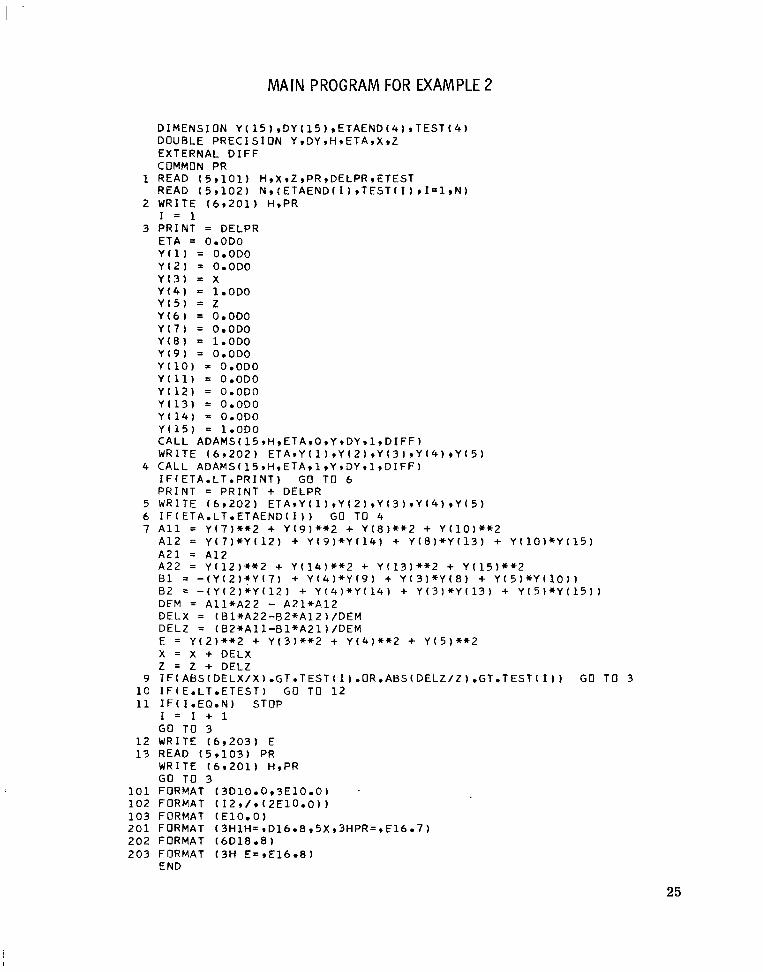
MAIN PROGRAM FOR EXAMPLE 2

DIMENSION Y ( ~ ~ ) ~ D Y ( ~ ~ ) ~ E T A E N D ( ~ ) ~ T E s T E S T ( ~ ) DOUBLE P R E C I S I O N Y ~ D Y I H ~ E T A ~ X S Z EXTERNAL D I F F COMMON PR

1 READ ( 5 9 1 0 1 ) HIXIZ~PRIDELPRIETEST READ ( 5 9 1 0 2 ) N I ( E T A E N D ( I ) ~ T E S T ( I ) , I P ~ ~ N )

2 WRITE ( 6 9 2 0 1 1 HIPR 1 = 1

3 P R I N T = DELPR ETA = 0oODO Y ( 1 ) = OoODO Y ( 2 ) = OoODO Y ( 3 ) = x Y ( 4 1 = l o O D 0 Y ( 5 ) = z Y ( 6 ) = 0oODO Y ( 7 ) = 0oODO Y ( 8 ) = 1oODO Y ( 9 ) = 0oODO Y ( 1 0 ) OoODO Y ( 1 1 ) = OoODO Y ( 1 2 ) = OoODO Y ( 1 3 ) = 0oODO Y ( 1 4 ) OoODO Y ( 1 5 ) = 1.ODO CALL A D A M S ( ~ S ~ H , E T A ~ O I Y I D Y ~ ~ ~ D I F F ) WRITE ( 6 , 2 0 2 ) E T A t Y ( l ) r Y ( 2 ) r Y 1 3 l r Y ( 4 ) , Y ( 5 )

4 CALL A D A M S ( ~ ~ ~ H ~ T E S E T A ~ ~ ~ Y ~ D Y , ~ , D I F F I I F ( E T A o L T o P R 1 N T ) GO TO 6 P R I N T = P R I N T + DELPR

5 WRITE ( 6 9 2 0 2 ) E T A I Y ( ~ ) ~ Y ( ~ ) ~ Y ( ~ ) , Y ( ~ ) ~ Y ( ~ ) 6 I F ( E T A o L T o E T A E N D ( 1 ) ) GO TO 4 7 A l l = Y ( 7 ) * * 2 + Y ( 9 ) * * 2 + Y ( 8 ) * * 2 + Y ( 1 0 ) * * 2

A12 = Y ( 7 ) * Y ( 1 2 ) + Y ( 9 ) * Y ( 1 4 ) + Y ( 8 ) * Y ( 1 3 ) + Y ( l O ) * Y ( 1 5 ) A 2 1 = A12 A 2 2 = Y ( 1 2 ) * * 2 + Y ( 1 4 ) * * 2 + Y ( 1 3 ) * * 2 + Y ( 1 5 ) * * 2 81 = - ( Y ( 2 ) * Y ( 7 ) + Y ( 4 ) * Y ( 9 ) + Y ( 3 ) * Y ( 8 ) + Y ( 5 ) * Y ( 1 0 ) 1 92 = - ( Y ( 2 ) * Y ( 1 2 ) + Y ( 4 ) * Y ( 1 4 ) + Y ( 3 ) * Y ( 1 3 ) + Y ( 5 ) * Y ( 1 5 ) ) DEM = A l l * A 2 2 - A 2 1 * A 1 2 DELX = ( B l * A 2 2 - B 2 + A 1 2 ) / D E M DEL2 = ( 8 2 * A l l - B l * A 2 1 ) / D E M E = Y ( 2 ) * * 2 + Y ( 3 ) * * 2 + Y ( 4 ) * * 2 + Y ( 5 ) * * 2 X = X + DELX Z = Z + DEL2

9 I F ( A B S ( D E L X / X ) o G T o T E S T ( I ) ~ O R o A B S ( D E L Z / Z ) o G T o T E S T ( I ~ ) GO T O 3 10 I F ( E o L T o E T E S T 1 GO T O 1 2 11 I F ( 1 o E Q . N ) STOP

I = 1 + 1 GO T O 3

1 2 WRITE ( 6 9 2 0 3 ) E 1 3 READ ( 5 9 1 0 3 ) PR

WRITE ( 6 9 2 0 1 ) H,PR GO TO 3

1 0 1 FORMAT ( 3 D 1 0 ~ 0 ~ 3 E l O o O ) 1 0 2 FORMAT ( I Z ~ T E S / ~ ( Z E ~ ~ O O ) ) 1 0 3 FORMAT ( E 1 0 . 0 ) 2 0 1 FORMAT ( 3 H l H = 9 D l 6 * 8 r 5 X 9 3 H P R = r E 1 6 . 7 ) 2 0 2 FORMAT ( 6 0 1 8 . 8 ) 2 0 3 FORMAT ( 3 H E = * E 1 6 * 8 )

END

25

L

C SUBROUTINE T O COMPUTE THE D I F F E R E N T I A L EQUATIONS OF EXAMPLE 2 SUBROUTINE D IFF(ETAIY ,DY) DOUBLE P R E C I S I O N ETAIYIDY D IMENSION Y ( l ) , D Y ( l ) COMMON PR D Y ( 1 ) = Y ( 2 ) D Y ( 2 ) = Y ( 3 ) D Y ( 3 ) = 2 0 O D O * Y ( 2 ~ * * 2 - 3 ~ O D O * Y ( 1 ~ * Y ( 3 ~ ~ Y ~ 4 ~ D Y ( 4 ) = Y ( 5 ) D Y ( 5 ) = - 3 . O D O * P R + Y ( l ) * Y ( 5 ) D Y ( 6 ) = Y ( 7 ) D Y ( 7 ) = Y ( 8 ) D Y ( 8 ) = 4.ODO*Y(2)*Y(7)-30ODO*(Y(3)*Y(6)+Y(l)*Y(8))-Y(9) D Y ( 9 ) = Y ( 1 0 ) D Y ( 1 0 ) = -3oODO*PR*(Y(5)+Y(6)+Y(l)*Y(lO)) D Y ( 1 1 ) = Y ( 1 2 ) D Y ( 1 2 ) = Y ( 1 3 ) D Y ( 1 3 ) = 4 0 O D O * Y ( 2 ) * Y ( 1 2 ) - 3 0 0 D O * ~ Y ( 3 ~ * Y ( 1 1 ~ + Y ~ 1 ~ * Y ~ 1 3 ~) - Y ( 1 4 ) D Y ( 1 4 ) = Y ( 1 5 ) D Y ( 1 5 ) = - 3 ~ O D O * P R * ( Y ( 5 ) * Y ( l l ~ + Y ( 1 ~ * Y ~ 1 5 ~ ) RETURN END

26

MAIN PROGRAM FOR EQUATIONS CONTAINING A PARAMETER

DIMENSION Y ( 9 ) , D Y ( 9 ) r E T A E N D ( 4 ) , T E S T ( 4 ) DOUBLE P R E C I S I O N Y 9 3 Y 9 ; i r E T A r X r B EXTERNAL D I F F COMMON B

1 READ ( 5 9 1 0 1 ) H ~ X S B I B H ~ B E N D I D E L P R I E T E S T READ ( 5 9 1 0 2 ) N I ( E T A E N D ( I ) I T E S T ( I ) I I = ~ ~ N )

2 WRITE ( 6 9 2 C 1 ) H 1 = 1

3 P R I N T = DELPR ETA = OoODO Y ( 1 ) = OoODO Y ( 2 ) = OoODO Y ( 3 ) = x Y ( 4 ) = OoODO Y ( 5 ) 5 OoODO Y ( 6 ) = 1.ODO Y ( 7 ) = O o C D O Y ( 8 ) = O - O D O Y ( 9 ) = O o O D O CALL A D A M S ( ~ , H I E T A I O ~ Y I D Y , ~ , D I F F ) WRITE ( 6 9 2 0 2 ) B ~ E T A ~ Y ( ~ ) , Y ( ~ ) P Y ( ~ )

4 CALL ADAMS(3,lirETArl,Yr3YrlrDIFF) IF (ETA.LT .PRINT) GO TO 6 P R I N T = P R I N T + DELPR

5 WRITE ( 6 9 2 0 3 ) E T A * Y ( l ) , Y ( Z ) r Y ( 3 ) 6 I F ( E T A m L T o E T A E N D ( 1 ) ) GO TO 4

DEM = Y ( 5 ) * * 2 + Y ( 6 ) * * 2 + Y ( R ) + * 2 + Y ( 9 ) * * 2 DELB = - ( ( Y ( 2 ) - 1 o O D O ) * Y ( 8 ) + Y ( 3 ) * Y ( ~ ) ) / D E M DELX = - ( ( Y ( 2 ) - 1 . O D O ) * Y ( 5 ) + Y ( 3 ) " Y ( b ) ) / D E M E = ( l . O D O - Y ( 2 ) ) * * 2 + Y ( 3 ) * * 2 X = X + DELX B = B + DELE

9 I F ( A B S ( D E L X / X ) . G T . T E S T ( I ) . O R . A B S ( D E L B / B ) . G T . T E S T ( I ) ) GO TO 3 10 I F ( E . L T o E T E S T ) GO TO 1 2 11 IF(1 .EQ.N) STOP

I = I + 1 GO T O 3

1 2 WRITE ( 6 r 2 0 4 ) E 13 I F ( B o G T o B E N D ) STOP 1 4 B = B + B H

X = X - B H * ( Y ( 5 ) * Y ( 8 ) + Y ( 6 ) * Y ~ 9 ) ) / r Y ( 5 ) * * 2 + Y ( 6 ) * * 2 ) GO TO 3

101 FORMAT ( 3 D 1 0 o 0 9 4 E l O o O ) 1 0 2 FORMAT ( 1 2 , / 9 ( 2 E l O o O ) ) 2 0 1 FORMAT ( 3 H l H = 9 3 1 6 * 8 ) 2 0 2 FORMAT ( 3 H B = r D 3 0 ~ 1 6 r / , 4 D 2 5 0 8 ) 2 0 3 FORMAT ( 4 D 2 5 . 8 ) 2 0 4 FORMAT ( 3 H E = r E 1 6 0 8 )

END

27

C SUBROUTINE TO COMPUTE THE D I F F E R E N T I A L EQUATIONS OF* EQUATIONS C C O N T A I N I N G A PARAMETER, EXAMPLE

SUBROUTINE D I F F ( E T A * Y , D Y ) DOUBLE P R E C I S I O N ETA,Y*DY,B D I M E N S I O N Y ( l ) s D Y ( l ) COMMON B D Y ( 1 ) = Y ( 2 ) D Y ( 2 ) = Y ( 3 ) D Y ( 3 ) = B * ( Y ( 2 ) * * 2 - 1 * 0 ) - Y ( l ) * Y ( 3 ) D Y ( 4 ) = Y ( 5 ) D Y ( 5 ) = Y ( 6 ) D Y ( 6 ) = 2 ~ 0 * B * Y ~ 2 ~ * Y ~ 5 ~ ~ Y ~ 4 ~ * Y ~ 3 ~ ~ Y ~ 1 ~ * Y f 6 ~ D Y ( 7 ) = Y ( 8 ) D Y ( 8 ) = Y ( 9 ) D Y ( 9 ) = - ( Y ( l ) * Y ( 9 ) + Y ( 7 ) + Y ( 3 ) ) + 2 . O * B * Y ( 2 ) * Y 1 8 ) + Y ( Z ) * * Z - l * O RETURN END

28

APPENDIX C

INTEGRATION SUBROUTINE

Description of Flow Chart

The numbers in the following description refer to flow chart box numbers (fig. 8) and formula numbers of FORTRAN listing.

1. Test to determine if subroutine is to be initialized or if it is to advance the solu­tion.

2. Test if subroutine is t o use Runge-Kutta or Adams-Moulton integration scheme. Subroutine always uses Runge-Kutta for the first three increments.

3. 4. 5. 6. 7. 8. 9.

Counter is initialized for Adams-Moulton scheme. Counter is initialized for Runge-Kutta scheme. Derivatives are evaluated at the initial value of the independent variable. Counter is tested. Counter is incremented by one. Counter is incremented by one. Counter is incremented by one.

ADAMS(7

-c t

3 9

1- K 2- K 3- K 4- K I 5- K

1 5

0Return Advance solution -

Figure 8. - Flw chart of integration subroutine.

29

10. Derivatives a r e evaluated at the proper values of the independent variable, and Runge-Kutta formulas are applied.

11. Derivatives are evaluated, and Adams-Moulton formulas are applied. Correc­tion equation is used once for each increment.

12. Solution is advanced one increment. This subroutine requires that a subroutine to compute the differential equations be

supplied. A discussion of integration equations used in this subroutine is given sub­sequently .

30

Integration Subroutine

C INTEGRATION SUBROUTINE FOR INTEGRATING SYSTEMS OF D I F F E R E N T I A L C EQUATIONS OF THE TYPE DY = F ( X , Y ) , BY RUNGE-KUTTA OR ADAMS-MOULTON C FORMULAS

SUBROUTINE A D A M S ( N , H , X I I S E T , Y , D Y I I N D E X ~ F ) DOUBLE P R E C I S I O N P,Y,YR,DYLLIDYLLL,DYLIDYIDYR~C~~C~~C~~X,H DIMENSION Y ( l ) r D Y ( l ) , P ( 2 4 ) r Y R ( 2 4 ) r D Y L L L o , D Y L L L ( 2 4 ) , ~ Y L L ( 2 4 ) ~ ~ Y L ( Z 4 ) ~ D Y R (

* 2 4 l , C 2 ( 2 4 ) , C 3 ( 2 4 ) r C 4 ( 2 4 ) 1 I F ( I S E T . G T . 0 ) GO TO 6 2 I F ( I N D E X . L E . 0 ) GO T O 4 3 K = 2

GO TO 5 4 K = 1 5 CALL F ( X I Y ~ D Y )

RETURN 6 GO TO ( 1 0 ~ 7 9 8 ~ 9 9 1 1 ) 9 K ~ 7 K = 3

GO TO 10 8 K = 4

GO T O 10 9 K = 5

10 DO 1001 I = l , N 1001 P ( I ) = Y ( 1 ) + ( H / Z . O D O ) * D Y ( I )

CALL F ( X + H / ~ . O D O I P * C ~ ) DO 1 0 0 2 I = l , N

1 0 0 2 P ( 1 ) = Y ( 1 ) + ( H / 2 . O D O ) * C 2 ( 1 ) CALL F(X+H/Z.ODO,P,C3) DO 1 0 0 3 I = l , N

1003 P ( 1 ) = Y ( I ) + H * C 3 ( 1 ) CALL F ( X + H * P w C 4 ) DO 1004 I = l , N

1004 Y R ( 1 ) = Y ( I ) + ( H / 6 ~ O D O ) * ( D Y ( I ) + 2 ~ 0 D O + C 2 ( I ) + 2 . O D O x C 3 ( I ) + C 4 ~ 1 ~ ~ CALL F(X+H,YR,DYR) GO TO 1 2

11 DO 1101 I = l r N 1101 P ( I ) = Y ( 1 ) + ~ H / 2 4 . O D 0 ~ * ~ 5 5 ~ O D O * D Y ~ I ~ ~ 5 9 ~ O D O * D Y L ~ I ~ + 3 7 ~ O D O * D Y L L

* ( 1 ) - 9 . 0 D O * D Y L L L ( I ) ) CALL F(X+HIP,DYR) DO 1 1 0 2 I = l r N

1 1 0 2 Y R ( 1 ) = Y ( I ) + ~ H / 2 4 . O D 0 ) * ~ 9 ~ O D O * D Y R ~ I ) + l 9 ~ O D O * D Y ~ I ~ ~ 5 ~ O D O * D Y L ~ I ~* + D Y L L ( I ) )

CALL F(X+H,YR*DYR) 1 2 X = X+H

DO 1 2 0 1 I = l r N Y ( I ) = Y R ( 1 ) D Y L L L ( 1 ) = D Y L L ( 1 ) D Y L L ( 1 ) = D Y L ( 1 ) D Y L ( 1 ) = D Y ( 1 )

1 2 0 1 D Y ( 1 ) = D Y R ( 1 ) RETURN END

31

- -

- - -

- -

Integ rat ion Form u la s

The formulas described here a r e used in the integration subroutine given in appen­dix B. Let the system of n first-order differential equations to be solved be given in the form

where f , y, and are n dimensional vectors. With initial conditions

let h be the increment of the independent variable x, with the notation x.J

= xo + jh. Then the Runge-Kutta formulas a r e (ref. 10):

- - 1 ­yj+l

= y.J

+ -6 (ko + 2E1 + 2k2 + 4 )

-where ko, k 1' k2, and k3 a r e n dimensional vectors and

-ko = hf(x.

J' y.)

J

-k l = hfcTj+1/2,Yj + f Eo)

and

__ ­k3 = hf(xj+l, yj + k2)

The Adams-Moulton predictor-corrector formulas of reference 10 a r e given by

--p = y.J + ­y ~ + l - h24 (55y!J - 59y;;_1 + 3 7 3 - 2 - 95-3)

32

where

and the superscripts P and C stand for predicted and corrected values, respectively.

33

REFERENCES

1. Fox, Leslie, ed. : Numerical Solution of Ordinary and Partial Differential Equations. Pergamon Pres s , 1962, ch. 5.

2. Radbill, John R. : Application of Quasilinearization to Boundary-Layer Equations. AIAA J. , vol. 2, no. 10, Oct. 1964, pp. 1860-1862.

3. Hartree, D. R. : Numerical Analysis. Clarendon P r e s s (Oxford), 1952, pp. 143-144.

4. Hartree, D. R. : On an Equation Occurring in Falkner and Skan's Approximate Treatment of the Equations of the Boundary Layer. Proc. Cambridge Phil. SOC., vol. 33, pt. 2, Apr. 1937, pp. 223-239.

5. Wylie, C. R. : Advanced Engineering Mathematics. McGraw-Hill Book Co., Inc. , 1951, pp. 530-531.

6. Yohner, Peggy L. ; and Hansen, Arthur G. : Some Numerical Solutions of Similarity Equations for Three-Dimensional Laminar Incompressible Boundary-Layer Flows. NACA TN 4370, 1958.

7. Smith, A. M. 0. : Improved Solutions of the Falkner and Skan Boundary-Layer Equation. Sherman M. Fairchild Fund Paper No. FF-10, Inst. Aeron. Sci. , Mar. 1954.

8. Ostrach, Simon (With appendix B by Lynn U. Albers): An Analysis of Laminar Free-Convection Flow and Heat Transfer About a Flat Plate Parallel to the Direction of the Generating Body Force. NACA Rept. 1111, 1953.

9. Tompkins, Charles B. : Methods of Steep Descent. Modern Mathematics for the Engineer, E. F. Beckenbach, ed., McGraw-Hill Book Co., Inc. , 1956, pp. 448-479.

10. Hildebrand, F. B. : Introduction to Numerical Analysis. McGraw-Hill Book Co. , Inc., 1956, pp. 199-239.

34 NASA-Langley, 1965 E-2959

“The aeronautical and space activities of the United StateJ Jhall be conducted so as to contribute . . . to the expansion of human knowl­edge of phenomena in the atmosphere and space. The Administration shall provide for the widest practicable and appropriate dirsemination of information concerning itJ activities and the reJulfJ thereof ,”

AERONAUTICS-NATIONAL AND SPACEACTOF 1958

NASA SCIENTIFIC AND TECHNICAL PUBLICATIONS

TECHNICAL REPORTS: Scientific and technical information considered important, complete, and a lasting contribution to existing knowledge.

TECHNICAL NOTES: Information less broad in scope but nevertheless of importance as a contribution to existing knowledge.

TECHNICAL MEMORANDUMS: Information receiving limited distri­bution because of preliminary data, security classification, or other reasons.

CONTRACTOR REPORTS: Technical information generated in con­nection with a NASA contract or grant and released under NASA auspices.

TECHNICAL TRANSLATIONS: Information published in a foreign language considered to merit NASA distribution in English.

TECHNICAL REPRINTS: Information derived from NASA activities and initially published in the form of journal articles.

SPECIAL PUBLICATIONS: Information derived from or of value to NASA activities but not necessarily reporting the results .of individual NASA-programmed scientific efforts. Publications include conference proceedings, monographs, data compilations, handbooks, sourcebooks, and special bibliographies.

Details on the availability o f these publications may be obtained from:

SCIENTIFIC AND TECHNICAL INFORMATION DIVISION

NATIONAL AERONAUTICS AND SPACE ADMINISTRATION

Washington, D.C. PO546