Satellite observations of mesoscale ocean features and

Satellite observations of mesoscale ocean features and copropagating

atmospheric surface fields in the tropical belt

Richard Justin Small, Shang-Ping Xie,1 and Jan HafnerInternational Pacific Research Center, School of Ocean and Earth Science and Technology, University of Hawaii, Honolulu,Hawaii, USA

Received 15 July 2004; revised 1 November 2004; accepted 4 January 2005; published 22 February 2005.

[1] Recent studies of air-sea interaction using satellite data have shown a high positivecorrelation between wind speed and sea surface temperature (SST) over mesoscale oceanfeatures in certain frontal regions. The aim of this study is to determine to what extentmesoscale ocean dynamics modifies the surface wind speed over the global tropicsbetween 40�S and 40�N. Cross-spectral and linear regression methods are used to identifyrobust relationships between ocean and atmospheric variables. The ocean dynamicalfeatures, measured by their sea surface height anomaly (SSHA), affect SST in a mannerconsistent with advection of the mean temperature gradient by anomalous currents. Theresponse varies from 0.2�C of SST per cm of SSHA near the equator to 0.05�C cm�1 athigher latitudes. A remarkably consistent in-phase relationship between SST and windspeed is found over the complete domain. Wind speed response varied from 0.5 to1.5 ms�1 per �C of SST change. This in-phase response of wind speed is consistent withprevious studies suggesting that the SST variations cause changes in the vertical exchangeof momentum and in the pressure gradient, which alter the wind speed.

Citation: Small, R. J., S.-P. Xie, and J. Hafner (2005), Satellite observations of mesoscale ocean features and copropagating

atmospheric surface fields in the tropical belt, J. Geophys. Res., 110, C02021, doi:10.1029/2004JC002598.

1. Introduction

[2] Basin-scale SST anomalies are often observed to benegatively correlated with the strength of prevailing winds[Mantua et al., 1997; Okumura et al., 2001; Liu et al.,1994]. Over the extratropical North Pacific and Atlantic,negative SST anomalies of the basin scale are a response tointensified westerly winds that increase the latent andsensible heat release from the ocean. Most of the anomalouswind forcing, however, is not induced by the in situ SSTchanges but is considered to result from internal atmo-spheric variability [Frankignoul, 1985; Barsugli andBattisti, 1998] or teleconnection from the tropics [Alexanderet al., 2002]. In the tropics, this negative correlation isindicative of a feedback between wind evaporation and SST[Chang et al., 2001; Xie and Tanimoto, 1998].[3] In contrast with the basin-scale relationship, recent

studies have shown that SST variability on frontal andmesoscale leads to a positive correlation of wind speedand SST [Xie et al., 2004]. For instance, Hayes et al. [1989],Chelton et al. [2001], and Hashizume et al. [2001] notedthat stronger winds were observed over the warm phase ofTropical Instability Waves (TIWs). Similar relationshipsbetween SST and wind speed were found to occur inmesoscale features in the Kuroshio [Nonaka and Xie,

2003; White and Annis [2003] (hereinafter referred to asWA03), Somali current [Vecchi et al., 2004], Antarcticcircumpolar current [O’Neill et al., 2003; WA03], Brazilcurrent and Gulf Stream (WA03). These results suggest thaton the small scales of the ocean mesoscale, it is the oceanthat is forcing the atmosphere, via the impact of the SST onthe planetary boundary layer mixing processes and pressuregradients [Xie, 2004], as discussed in more detail in section4.2.1.[4] These findings give rise to the question of whether the

relationship between winds and SST is a robust and generalfeature of ocean mesoscales. This paper aims to answer thisquestion, and to investigate the origin of the SST variability,using satellite data. The region of analysis is limited by theavailability of multiyear microwave imager (cloud-transpar-ent) SST for tropical regions only. (The recent launch of theAQUA satellite with the AMSR-E instrument gives poten-tial to use microwave imager data to study the global ocean.However, only two complete years of data are currentlyavailable, too short for the analysis.) The tropical beltbetween 40�S and 40�N (see Figure 1) has been surveyedsince December 1997 by the Tropical Rainfall MeasuringMission (TRMM) satellite, on board which the TRMMMicrowave Imager (TMI) detects SST. The analysis herewill extend the above studies, to include variability over themajor ocean basins equatorward of 40� using multiyear datasets.[5] The variables to be studied here are the sea surface

height anomaly (SSHA), the SST, and the wind speed. Therelationship between SSHA and SST is shown to indicatehow ocean dynamics is related to the surface temperature

JOURNAL OF GEOPHYSICAL RESEARCH, VOL. 110, C02021, doi:10.1029/2004JC002598, 2005

1Also at Department of Meteorology, School of Ocean and EarthScience and Technology, University of Hawaii, Honolulu, Hawaii, USA.

Copyright 2005 by the American Geophysical Union.0148-0227/05/2004JC002598$09.00

C02021 1 of 19

variability. In general, the SST field is influenced by surfaceheat fluxes (sensible and latent), short and long waveradiation fluxes, and mixing and advection in the ocean.For the relatively short, propagating oceanic features beingconsidered in this paper, it is expected that SST change willbe governed either by advection of mean SST by eddycurrents, or by entrainment from the thermocline into themixed layer when the thermocline is shallow [Hill et al.,2000].[6] These two effects governing the relationship of

SSHA and SST can be distinguished by studying thephase difference between the two quantities, as discussedin section 4.1.1. Previous studies have shown some

conflicting results. For instance, WA03 found that SSTand SSHA were collocated in the eddies of their study,based on an analysis of a limited number of snapshots.Polito et al. [2001] investigated Tropical InstabilityWaves and found SSHA led the SST by 90� (in a narrow2� latitude band) and used this to infer that advection ofmean SST dominated SST variations. This contrastedwith previous results showing SST led SSHA by up to90�, in the analysis of tropical Rossby waves by White[2000], and an analysis of south Indian Ocean waves byQuartly et al. [2003]. In the present study we willprovide robust estimates of the relationship between thetwo variables from the multiyear data sets.

Figure 1. Standard deviation of ocean and atmospheric variables, filtered as discussed in section 2.1.(a) Sea surface height anomaly (SSHA) (color, cm) from October 1992 to August 2001. Overlaid are the5� latitude boxes making up the south Indian Ocean (white grid), west Pacific (black grid), east Pacific(white grid, overlapping), and Atlantic (black grid) domains. (b) Sea surface temperature (SST) (color,�C), from TRMM TMI, from December 1997 to March 2003. Overlaid is the mean SST from the sameperiod, at intervals of 3�C. (c) Wind speed (color, ms�1), from QuikSCAT, 21 July 1999 to March 2003.Overlaid are the mean wind vectors (ms�1).

C02021 SMALL ET AL.: OBSERVATIONS OF AIR-SEA INTERACTION

2 of 19

C02021

[7] The paper is organized as follows. Section 2presents the data sets and methods. In section 3 thestandard deviation of the mesoscale features are analyzed,in fields of SSHA, SST and in wind speed, to identify thekey regions of variability. Section 4 presents the charac-teristics of multiyear air-sea interaction as determinedfrom linear regression and cross-spectral methods.Section 5 contains a discussion of the results and Section 6gives the conclusions.

2. Data and Methods

2.1. Satellite Data

[8] This study uses the TMI SST (version 3a) availablefrom December 1997, and QuiKSCAT scatterometer vectorwinds, available since July 1999, processed by RemoteSensing Systems http://www.ssmi.com) onto a 0.25� grid.TMI data is not affected by clouds (except under heavyprecipitation) and hence has a significant advantage overinfrared radiometers in regions of large cloud cover (such asthe stratus decks in the tropical eastern oceans, and thestorm track regions). The radar backscatter (or cross section)measured by scatterometers is most directly related to thestress on the ocean surface, which induces the wavesdetected by the radar. The wind stress is dependent on windspeed, surface current, and near-surface static stability, sothat for example, a particular value of wind stress cancorrespond to different wind speeds under different stabilityconditions. For this reason the radar cross section is cali-brated to equivalent neutral stability winds at 10 m, U10n

[Wentz and Smith, 1999]. In a comprehensive investigationof collocated QuikSCAT measurements and mooring datafrom over 100 buoys (buoy data were from the NationalData Buoy Center, the TAO array, the Pilot ResearchMoored Array in the tropical Atlantic and the JapanMeteorological Agency), Ebuchi et al. [2002] found thatthere was no significant dependence of QuikSCATminus buoy U10n on either SST or on air-sea temperaturedifference.[9] Daily output is obtained from a 3 day running mean

of data to improve the coverage. We further average the datato produce a weekly data set. In off-equatorial regions thisaveraging does not significantly degrade the resolution offeatures of interest (with periods of 100 days or more), butnear the equator it may impact on short, 20–30 day periodTIWs. However, for general consistency, the weekly aver-age is applied everywhere. (For the TIWs, the results havebeen validated against analysis at daily resolution wherepossible).[10] Sea level data is gathered in the form of combined

TOPEX/POSEIDON and European Remote Sensing sat-ellite SSHA from Centre National d’Etudes Spatiales(CNES) Archiving, Validation and Interpretation of Sat-ellite Oceanographic data (AVISO [Ducet et al., 2000]),from October 1992, on a 0.25� grid, every 10 days. (Forcomparison of SSHA and SST, the SST fields are linearlyinterpolated in time onto the time of the SSHA output.)The following time periods were studied in the jointanalysis: for SSHA and SST, December 1997 to March2003; for SST and wind speed, July 1999 to March 2003.For analysis of one data set alone, we use the completedata set up to March 2003.

[11] In order to focus on mesoscale variability, a runningaverage over 10� of longitude is removed, as are a runningaverage over 40 weeks and the first three annual harmonics.The domain of interest is determined by the TRMM datacoverage and is shown in Figure 1.

2.2. Cross Spectra

[12] In this study spectral Fourier analysis is used toexamine waves occurring in different types of satellite dataand their relationships. Fourier analysis was chosen as itprovides a clear method of summarizing changes in wavecharacteristics and relationships with latitude. In contrastwith the Radon transform [Hill et al., 2000] it has the abilityto identify wavelengths and period as well as phase speed.The need here to provide short summaries of wave charac-teristics precludes the use of finite-impulse-response filters[Polito and Liu, 2003] or wavelet analysis [Cromwell, 2001],which introduce added dimensions (a time and/or spacedependence) into the spectra. Although there are well knownlimitations of applying fast Fourier transform (FFT) tech-niques to determine wave characteristics, particularly inrespect of nonstationary features, the FFT approach is takenhere as our main aim is not to accurately and preciselydetermine spatial and temporal characteristics (as done by,e.g., Polito and Liu [2003] and Chelton and Schlax [1996]),but to focus instead on the phase and response relationshipbetween quantities in an overall sense. The validity of thisFFT approach is investigated here by comparing against alocal analysis performed using linear regression (seesection 2.4).[13] In brief, the cross-spectral analysis technique com-

pares and correlates the Fast Fourier Transforms (FFTs) oftwo variables. Following the notation of Emery andThomson [1998] (hereinafter referred to as ET98), the quan-tities used here are the cross-amplitude spectrum A12(k, w)(ET98, equation 5.8.13), describing the joint variability for aparticular frequency w and zonal wave number k, regardlessof phase relationship; the coherence spectrum g12

2 (k, w)(ET98, equation 5.8.21), which gives a value between 0and 1 of the coherence (squared) between two variables; theresponse function H12(k, w) (ET98, equation 5.8.33), whichdescribes the magnitude of the second variable whichresponds to unit amount of the first variable; and finally thephase spectrumF12(k,w) (ET98, equation 5.8.13), describingthe phase difference between the two variables of interest.(The convention here is that positive phase difference impliesthe first array leads the second array.)[14] It is important to note that in order to get a confident,

realistic value of coherence, some smoothing must beapplied. The smoothed coherence spectrum is given by

g212 k;wð Þ ¼ Q k;wð Þh i2þ Co k;wð Þh i2

F1* k;wð ÞF1 k;wð Þh i � F2* k;wð ÞF2 k;wð Þh i ;

Q k;wð Þ ¼ �= F1* k;wð ÞF2 k;wð Þð Þ;

Co k;wð Þ ¼ < F1* k;wð ÞF2 k;wð Þð Þ;

ð1Þ

where angled brackets denote a smoothing over spectralcomponents, F1(k, w) and F2(k, w) are the Fouriercomponents of the two variables, and = and < denoteimaginary and real parts. Confidence limits can bedetermined from the number of degrees of freedom in the


3 of 19

C02021

smoothed spectra. Following ET98, if (1 � a) is the (1 �a)100% confidence interval we require, then the confidencelimit is given by

g2 ¼ 1� a2= DOF�2ð Þ: ð2Þ

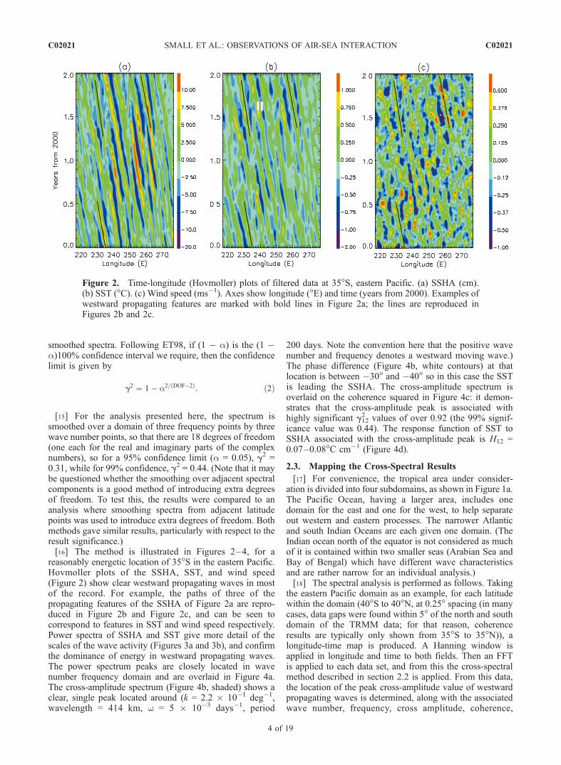
[15] For the analysis presented here, the spectrum issmoothed over a domain of three frequency points by threewave number points, so that there are 18 degrees of freedom(one each for the real and imaginary parts of the complexnumbers), so for a 95% confidence limit (a = 0.05), g2 =0.31, while for 99% confidence, g2 = 0.44. (Note that it maybe questioned whether the smoothing over adjacent spectralcomponents is a good method of introducing extra degreesof freedom. To test this, the results were compared to ananalysis where smoothing spectra from adjacent latitudepoints was used to introduce extra degrees of freedom. Bothmethods gave similar results, particularly with respect to theresult significance.)[16] The method is illustrated in Figures 2–4, for a

reasonably energetic location of 35�S in the eastern Pacific.Hovmoller plots of the SSHA, SST, and wind speed(Figure 2) show clear westward propagating waves in mostof the record. For example, the paths of three of thepropagating features of the SSHA of Figure 2a are repro-duced in Figure 2b and Figure 2c, and can be seen tocorrespond to features in SST and wind speed respectively.Power spectra of SSHA and SST give more detail of thescales of the wave activity (Figures 3a and 3b), and confirmthe dominance of energy in westward propagating waves.The power spectrum peaks are closely located in wavenumber frequency domain and are overlaid in Figure 4a.The cross-amplitude spectrum (Figure 4b, shaded) shows aclear, single peak located around (k = 2.2 � 10�1 deg�1,wavelength = 414 km, w = 5 � 10�3 days�1, period

200 days. Note the convention here that the positive wavenumber and frequency denotes a westward moving wave.)The phase difference (Figure 4b, white contours) at thatlocation is between �30� and �40� so in this case the SSTis leading the SSHA. The cross-amplitude spectrum isoverlaid on the coherence squared in Figure 4c: it demon-strates that the cross-amplitude peak is associated withhighly significant g12

2 values of over 0.92 (the 99% signif-icance value was 0.44). The response function of SST toSSHA associated with the cross-amplitude peak is H12 =0.07–0.08�C cm�1 (Figure 4d).

2.3. Mapping the Cross-Spectral Results

[17] For convenience, the tropical area under consider-ation is divided into four subdomains, as shown in Figure 1a.The Pacific Ocean, having a larger area, includes onedomain for the east and one for the west, to help separateout western and eastern processes. The narrower Atlanticand south Indian Oceans are each given one domain. (TheIndian ocean north of the equator is not considered as muchof it is contained within two smaller seas (Arabian Sea andBay of Bengal) which have different wave characteristicsand are rather narrow for an individual analysis.)[18] The spectral analysis is performed as follows. Taking

the eastern Pacific domain as an example, for each latitudewithin the domain (40�S to 40�N, at 0.25� spacing (in manycases, data gaps were found within 5� of the north and southdomain of the TRMM data; for that reason, coherenceresults are typically only shown from 35�S to 35�N)), alongitude-time map is produced. A Hanning window isapplied in longitude and time to both fields. Then an FFTis applied to each data set, and from this the cross-spectralmethod described in section 2.2 is applied. From this data,the location of the peak cross-amplitude value of westwardpropagating waves is determined, along with the associatedwave number, frequency, cross amplitude, coherence,

Figure 2. Time-longitude (Hovmoller) plots of filtered data at 35�S, eastern Pacific. (a) SSHA (cm).(b) SST (�C). (c) Wind speed (ms�1). Axes show longitude (�E) and time (years from 2000). Examples ofwestward propagating features are marked with bold lines in Figure 2a; the lines are reproduced inFigures 2b and 2c.


4 of 19

C02021

Figure 3. Power spectra for filtered data: (a) SSHA (cm2, log10 units) and (b) SST (�C2, log10 units).Note the convention that positive wave numbers denote westward moving. Eastern Pacific, 35�S. Blankareas fall below color bar values.

Figure 4. Cross-spectrum results for SSHA and SST, 35�S, eastern Pacific shown in Figure 1.(a) Power spectrum of SSHA (10�2 cm2, color) and of SST (10�4 �C2, white contours). (b) Cross-amplitude spectrum (10�5 cm2 �C2, color) and phase spectrum (degrees, white contours (the negativevalues denote SST leading SSHA)). (c) Coherence squared (color) and cross amplitude (10�5 cm2 �C2,bold contours, interval 0.5). (d) Response function (color, �C cm�1) and cross amplitude (10�5 cm2

�C2, bold contours).


5 of 19

C02021

phase, and response function. (The data set was dominatedby westward propagating waves, in agreement with previ-ous results from Chelton and Schlax [1996], Hill et al.[2000], and many others. For simplicity, we describe onlythese waves.) Finally, the median from the five degrees oflatitude in each box in Figure 1a is applied, to removeisolated spikes. This data is used to produce plots of spectralquantities against latitude.[19] In addition to the covariability results, a by-product

of the spectral analysis is the determination of the charac-teristic wave number, frequency, and derived phase speed ateach latitude in each domain. These results are presented inAppendix A and used for later reference.

2.4. Linear Regression

[20] To supplement the cross-spectral calculations, linearregressions have been performed in some limited regions toconfirm and illustrate more clearly the spatial relationshipsbetween the ocean and atmospheric variables. The regres-sion describes the relationship between a reference variable(such as SST) at a fixed point, and the variable of interest.Following Hashizume et al. [2001], a number of regressionmaps were compiled with reference points within 2� longi-tudinally of the central point, then a composite compiled bytaking the mean of each map with the reference pointsmatched. This was done to remove a small amount of noisein each individual map. The linear regressions are per-formed using 3 years of weekly data, from mid-July 1999to mid-July 2002. The results of the local regressionanalysis are generally consistent with those of the globalspectral analysis (section 4).

3. Spatial Patterns of Standard Deviation

[21] In this section the variability of each individualcomponent under consideration (SSHA, SST and windspeed) is discussed, in order to determine where the mostenergetic mesoscale features occur. Results are presented interms of the temporal standard deviation over the full recordof each component, filtered in time and space.

3.1. Sea Surface Height Anomaly (SSHA)

[22] Figure 1a shows the SSHA standard deviation acrossthe tropical belt of interest to this study, derived from10.5 years of data (October 1992–March 2003). Thestandard deviation plot allows identification of the mainregions of ocean mesoscale activity which will be studied indetail in the next section. The features in Figure 1a confirmand extend the analyses of Stammer [1997] and Ducet et al.[2000], the latter based on the first 6 years of mergedTOPEX/POSEIDON and ERS satellite data.3.1.1. Pacific Ocean[23] In the North Pacific, two main bands of high stan-

dard deviation (s) extend eastward from the western bound-ary, centered on 22�N (6 < s < 18 cm) and 30�–35�N (12 <s < 24 cm). The northern band is associated with theKuroshio/Kuroshio Extension (KE) and the southern onewith the Subtropical countercurrent (STCC [Qiu, 1999]) andthe Hawaiian Lee countercurrent (HLCC [Xie et al., 2001;Kobashi and Kawamura, 2001]) west and east of theDateline, respectively. A weaker band (3 cm < s < 6 cm)centered around 7�N near the western boundary is associ-

ated with the north equatorial current (NEC)/north equato-rial countercurrent (NECC). In the South Pacific, a broadregion of moderate standard deviation (3 < s < 9 cm)extends eastward from the eastern Australia coast acrossmost of the basin, between 20� and 30�S in the west andthen tilting southeastward to a meridional extent of 30� and40�S in the east; at the far west at least the standarddeviation is partly due to east Australian current eddies(12 < s < 24 cm). This broad band across the Pacific Oceanis referred to here as the South Pacific Waveguide, and isalso related to the south tropical countercurrent of Merle etal. [1969] and Qiu and Chen [2004]. Note that the vari-ability in this region and others discussed later may be dueeither to instabilities of the mean state, or due to propagationof free waves (both introducing temporal variance). Thispaper does not aim to distinguish between the possiblecauses of SSHA variability, and the zonally elongated zonesof high variability will be referred to as waveguides, withthe caveat that instability may also be contributing to thevariance.[24] In the central Pacific, a local maximum (3 < s <

6 cm) of a few degrees latitudinal extent centered around5�N is due to TIWs [Legeckis, 1977] on the northern edgeof the Cold Tongue. (There is also a weaker signature ofTIWs at 5�S on the southern edge of the Cold Tongue, notvisible in Figure 1a). In the eastern Pacific, moderatestandard deviation (3 < s < 9 cm) regions are located closeto the coast associated with the California current off NorthAmerica and the Humbolt current off South America, andwest of Central America in the vicinity of the Costa RicanDome [see Kessler et al., 2003] and upwelling regionsassociated with gap wind jet variability (such as the Gulfsof Tehuantepec [Chelton et al., 2000], Papagayo, andPanama). Across the open Pacific Ocean the standarddeviation is low (s < 3 cm) between 15�S and the equator.3.1.2. Atlantic Ocean[25] In the Atlantic the highest standard deviation can be

seen associated with the Gulf Stream (GS) and its eastwardextension north of Cape Hatteras (12 < s < 24 cm), and the‘‘North Atlantic Waveguide’’ at 34�N [Cromwell, 2001]composed of eddies along the Azores current [Pingree,2002; Mourino et al., 2003] which extends almost to theEuropean coast; also offshore of the Amazon associatedwith north Brazil current eddies (12 < s < 30 cm) [Garzoliet al., 2004]; and an eastward extension from the SouthAmerican coast at 5�N (3 < s < 9 cm), related possibly toshear between the equatorial currents (NEC, NECC) respec-tively; in a broad band about 5� latitude wide centered at30�S spanning the Atlantic (3 < s < 9 cm), related to theregion of cut-off eddies from the Agulhas retroflection[Garzoli et al., 1999; Schouten et al., 2000] extendingdown to 40�S near the tip of South Africa (where 12 <s < 30 cm), referred to here as the South Atlantic Wave-guide (previously observed by Ducet et al. [2000]); andlarge standard deviation off Argentina south of 30�S (12 <s < 18 cm) associated with the Brazil current and itsconfluence with the Malvinas current [Goni et al., 1996].3.1.3. South Indian Ocean[26] The southern part of the Indian Ocean exhibits

moderate standard deviation (3 < s < 9 cm) across thebasin between 20� and 30�S. This band, studied by Morrowand Birol [1998], appears related to the Leeuwin current


6 of 19

C02021

eddies off western Australia, 25�–30�S [Fang and Morrow,2003], propagating westward from their generation point.This band will be referred to here as the South IndianWaveguide. Moderate eddy variability (6 < s < 9 cm) is alsolocated just south of the Indonesian arc, centered at 12�S,where Perigaud and Delecluse [1992] found evidence of astrong annual Rossby wave, and Feng and Wijffels [2002]found strong intraseasonal standard deviation associatedwith the SEC and the Indonesian throughflow; and theAgulhas retroflection south of 35�S (note the Agulhas andMozambique currents, associated with s > 12 cm, are notincluded in the covariability analysis below).

3.2. Sea Surface Temperature (SST)

[27] For comparison, the standard deviation of filteredSST and the mean SST is shown in Figure 1b. Many, but notall, of the features seen in SSHA standard deviation inFigure 1a are reproduced in the SST standard deviation. Inregions where high SSHA standard deviation coincides witha mean SST gradient, there is high SST standard deviation,suggesting temperature advection by geostrophic currents(e.g., in the Gulf Stream region, and around most of theother western boundary currents, where s > 0.6�C. Notethat although currents in eddies are roughly in steadygeostrophic balance with SSHA, the propagation of theeddies causes variations in time which give rise to the SSTvariability.) High SST standard deviation (s > 0.5�C) is alsoassociated with the STCC, the California current, peaking at20�N, extending westward in the mean SST gradient, andassociated with the gap wind jets off Central America whichcause significant upwelling and eddies as discussed above.Further, the broad bands of energy across the ocean basinsidentified above as the South Indian Waveguide and SouthPacific Waveguide are seen in both quantities, wheretypically s > 0.4�C, while the South Atlantic Waveguidein the Atlantic has a more northwest-southeast tilt in theSST field than in the SSHA possibly due to the distributionof mean SST gradient. More notable differences are that theTIW standard deviation is high (s > 0.5�C) and dominatesthe equatorial eastern Pacific and Atlantic Oceans in theSST, at around 2�N (lying along the mean SST fronts),while features such as eddies in the Bay of Bengal and thoseassociated with the HLCC in the North Pacific, the NEC/NECC and SEC in the Atlantic and Indian Oceans haverelatively weak signatures in the SST standard deviation dueto the weak mean SST gradients there.

3.3. Wind Speed

[28] Next the wind speed standard deviation (Figure 1c)may be compared with the oceanic surface variables(Figures 1a and 1b). The wind speed standard deviationmirrors many of the features seen in the SSHA standarddeviation (Figure 1a), and, more particularly, the SST stan-dard deviation (Figure 1b). High standard deviation of windspeed (s> 0.5ms�1) can be seen extending eastward from themajor western boundary currents, and at the location ofTIWs, and over the southern ocean waveguides, the SouthAtlantic Waveguide, South Pacific Waveguide, and SouthIndian Waveguide (but in the Indian Ocean the standarddeviation in wind speed is maximum at more southernlatitudes (30� to 40�S) than seen in the SST and SSHAstandard deviation). The near-coincidence of these features

in the SST and wind speed standard deviation suggests thaton the scales of interest here, the wind speed is stronglyreacting to the oceanic mesoscale features. However somepurely atmospheric features are seen in the wind speed map:the ITCZ is marked as an area of high wind speed standarddeviation (s > 0.4 ms�1), particularly in the Pacific Oceancentered around 5�N. (In fact, some aspects of Figure 1cresemble the distribution of highest precipitation in rainfallclimatologies [see, e.g., Adler et al., 2001], suggesting thatconvective systems are also contributing to the wind speedvariability at these length and timescales. However, theseconvective systems will have very different phase speeds tothe ocean mesoscale features and so do not contribute to thejoint SST–wind speed variability discussed below.) Thestandard deviation of wind speed is also high in many coastalareas, and around islands such as the Hawaiian Islands. Thiscoastal variance maximum is due to variability of coastalwinds, with a mean speed which weakens toward the shore.Some of this coastal wind variability may be forced by SSTvariability, but it requires an along-coast filtering to extract,rather than the zonal filter used here. The coastal variabilityanalysis is beyond the scope of this paper.

4. Joint Variability Results

[29] In this section the joint variability of the ocean andatmospheric fields presented in section 3 is discussed.Firstly, the SSHA is related to the SST in section 4.1, andsecondly the SST is related to wind speed in section 4.2. Inboth sections, a brief review of possible physical mecha-nisms governing the relationships is given before the resultsare shown.

4.1. SSHA and SST Covariability

[30] The relationship between SSHA and SST is impor-tant in determining how the variable of importance to air-seainteraction (SST) is related to the ocean dynamics governedby SSHA. SST signatures of long SSHA waves may arisefrom two mechanisms: either by compression or stretchingof the near surface layer, or by meridional advection of themean temperature gradient [Hill et al., 2000].4.1.1. SST Equation[31] The dominant terms in the equation relating SST and

SSHA may be written as

@T 0

@T¼ �v0

@T

@yþ ah0 � nT 0; ð3Þ

where T is the SST, h is the SSH, v is the meridional current,a is the effect of mixed layer depth on the SST throughentrainment processes, n is a linear damping coefficient,overbars denote a timemean, and primes denote the deviationfrom that mean. Here it is assumed that the dominant meanSST gradients are in the meridional direction (a reasonableassumption for most of the domain (see Figure 1b)).Coefficient a is positive: a negative SSH perturbationimplies a shoaling thermocline and a consequent cooling ofthe SST if the thermocline is shallow enough and entrainmentprocesses are active. A function of ocean mean state, thisthermocline feedback is large in the eastern equatorialoceans, the tropical south Indian Ocean, and coastalupwelling regions (see Wang et al. [2004] for a review).


7 of 19

C02021

[32] The observed relationship between SSHA and SSTshown below will be compared with a simple model.Adapting Killworth and Blundell [2003, Appendix C] toinclude the effect of mixed layer depth on the SST, underthe assumption of a planar wave form

h0 ¼ h0 exp iqð Þ T 0 ¼ T0 exp iqð Þ; ð4aÞ

with q = kx � wt and geostrophic currents

v0 ¼ g

fh0x; ð4bÞ

where subscripts denote differentiation, and the relationshipbetween SST and SSHA is given by

T0

h0¼

� g

fikTy þ a

�iwþ 1

t

� � ; ð5Þ

where t = 1/n is the damping timescale. We may considerthe following four special cases.[33] 1. The advection-dominant case, wt 1:

T0

h0¼ g

f wkTy: ð6aÞ

SSHA and SST are in (out of) phase when Ty/f < 0(Ty/f > 0) for westward propagating waves (k < 0).[34] 2. The advection and damping case, wt � 1:

T0

h0¼ � g

fikTyt: ð6bÞ

For k < 0, the phase of T0 compared to h0 becomes p/2 �sgn(Ty)/sgn( f ) [Killworth and Blundell, 2003].[35] 3. The mixed layer depth effect dominant case:

T0

h0¼ ia

w: ð6cÞ

SST lags SSHA by 90�.[36] 4. The mixed layer and damping case:

T0

h0¼ at: ð6dÞ

SST and SSHA are in phase.[37] As seen in Figure 5, Ty < 0 over most of the Northern

Hemisphere oceans. Hence in the majority of the NorthernHemisphere, advection alone (6a) would lead to SST andSSHA in phase, and the addition of damping (6b) wouldcause SST to lead SSHA. Note also that under the effects ofadvection (6a) the response will be high near the equator,where f! 0, and there are large mean temperature gradientsTy in the Pacific and Atlantic associated with the ColdTongues (see Figure 1b).[38] These theoretical predictions will be compared next

with the observed joint variability of SSHA and SST.

4.1.2. Linear Regression[39] The linear regression results from a few selected

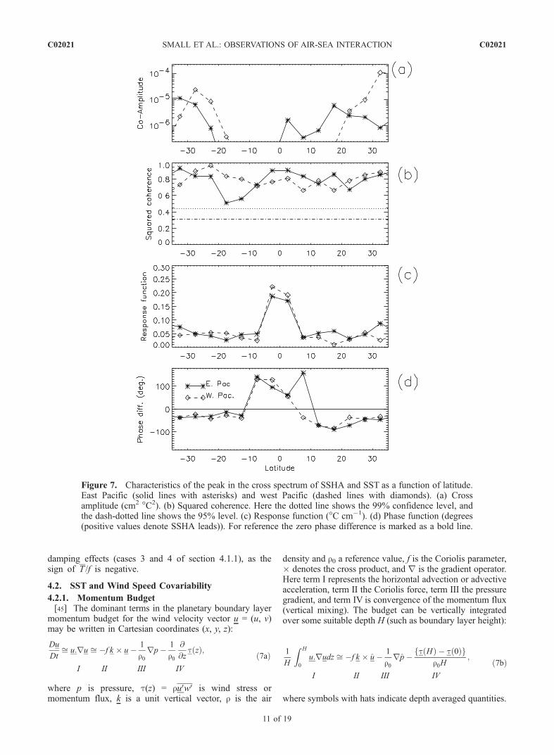
areas introduce the observed relationship between SSHAand SST. Here the regression is onto the SST at the locationslisted in the caption. Two regional examples, from the KEregion and the southern Indian Ocean, serve to illustrate thetypical case. In the KE region (Figure 6a), the anticyclone(shading denotes the SSHA) advects cool water southwardon its eastern flank, leading to cooling, and warm waternorthward on its western flank, leading to warming (theSST is shown as contours). In the south Indian Ocean(Figure 6b), the anticyclone advects cool water northwardon its eastern flank, leading to cooling, and warm watersouthward on its western flank, leading to warming. On itsown this effect would result in the SST centers overlying theSSHA centers. However, the SST centers in Figures 6a and6b are found just west of the SSHA centers, as confirmed inthe following coherence analysis, showing that SST leadsthe SSHA for the westward propagating waves, possiblydue to the thermal damping mentioned above.4.1.3. Cross Amplitudes, Response Function, andCoherence[40] In the eastern Pacific the largest cross amplitudes

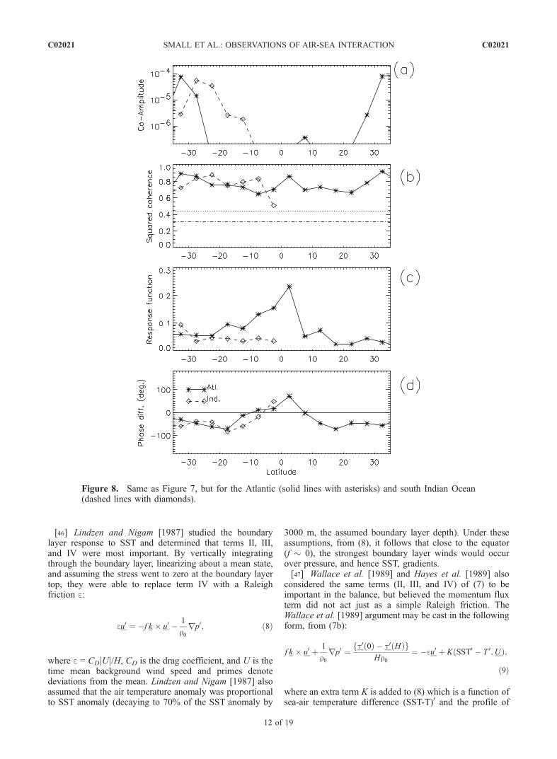
A12(k, w) (Figure 7a, solid line) are in the South PacificWaveguide, and between 2� and 5�N (TIW), and around18�–20�N (due to California current eddies and the east-ernmost influence of the HLCC). In the western Pacific(Figure 7a, dashed line), the highest A12(k, w) are in theSouth Pacific Waveguide, STCC and KE. Negligible crossamplitudes are observed in the Pacific Ocean between 20�Sand the equator. In the Atlantic ocean (Figure 8a, solid line),the largest A12(k, w) are found in the South AtlanticWaveguide and associated with the GS, and there is aweaker local maximum at 8�N associated with NEC/northBrazil current eddies. (Note that TIWs have a smallersignature in the Atlantic, possibly because of their shortdevelopment season: June–August [Hashizume et al.,2001]. This may help explain why their signal in SSHA islow (see Figure 1a), and consequently so is the covariabilityof SSHA and SST.) However, as will be seen below,Atlantic TIWs are prominent in the SST–wind speedcovariability, as they contribute significantly to equatorialSST and wind speed standard deviation, see Figures 1b and1c.) The highest A12(k, w) in the south Indian Ocean(Figure 8a, dashed line) lie in the South Indian Waveguide,and minimum values lie close to the equator. The coherencespectrum associated with these dominant features is high(0.7–0.9) and significant at 99% (Figures 7b and 8b).[41] Both the response function and the phase difference

change markedly around 10� from the equator. The responsefunction H12 is typically largest near the equator at around0.25�C cm�1 (Figures 7c and 8c, solid lines) in the Pacificand Atlantic Oceans, due to the small f and high jTyj just offthe equator (Figure 5a), as discussed above. Poleward of10� of the equator the response is smaller and between 0.05and 0.1�C cm�1 in the Pacific and Atlantic oceans(Figures 7c and 8c, solid lines). In contrast the responsefunction in the Indian Ocean changes little with latitude andremain around 0.05�C cm�1 (Figure 8c, dashed line). (Notethat in the Indian Ocean the equatorial region exhibits aminimum in magnitude of Ty(Figure 5a), in contrast to thecase in the Pacific and Atlantic, and this may counteract any


8 of 19

C02021

influence of the large geostrophic currents in this region ofsmall value of f. The response functions derived from thecross-spectral analysis (Figures 7c and 8c) are generallyconsistent with those derived from linear regression(Figure 6; note that the reciprocal of the regression shouldbe compared with the spectral analysis as the regression isSSHA onto SST). Precise differences between the methodsarise from the narrow band nature of the spectral methodand the broad band nature of the regression method.)4.1.4. Phase Difference[42] The phase difference function F12 (Figures 7d and

8d) shows many interesting features. For instance, around10� latitude the phase difference in the east Pacific changesdramatically (Figure 7d, solid line), from SSHA leading SSTequatorward of 10� to SST leading SSHA poleward of 10�.This is consistent with the influence of advection anddamping (case 2 of section 4.1.1) which predicts that thephase difference is p/2 � sgn(Ty/f ), which is positive closeto the equator and then changes sign somewhere between 6�and 10� both north and south of the equator in the eastPacific (see Figure 5b, and see also Figure 6c). (Note thatwhen the damping is weak, the advection mechanism

predicts an out-of-phase relation in the region where(Ty/f ) > 0, similar to the value observed at 7�N in Figure 7d.)[43] In the high southern latitudes of the east Pacific

(Figure 7d, solid line), the phase varies between �10� and�40� (i.e., SST leads SSHA). Between 15� and 20�N thedifference is between �90� and �80�, and at highernorthern latitudes it lies between �50� and 0� (SST leadsSSHA). The phase difference results outside of the equato-rial region are consistent with the advection and dampingargument, with SST leading SSH in regions of Ty/f < 0. Thephase difference results in this region are also consistentwith the linear regressions of Figures 6a and 6b.[44] The phase difference results from the other regions

(Figures 7d and 8d) also follow the trend of SSHAleading SST in the equatorial region, switching to SSTleading in higher latitudes. In the western Pacific and theAtlantic Ocean this is again consistent with the advectionand damping mechanism, as the sign of T /f changes afew degrees off the equator (Figure 5). In the southIndian Ocean the higher latitude results are consistentwith advection and damping, but the fact that SSHAleads SST at 2�S is more consistent with mixed layer and

Figure 5. Meridional gradient of mean SST, from the data set in Figure 1b, in units of 10�5 �C m�1

(approximately �C per degree of latitude). The bold white line marks the zero contour. (a) Distributionfrom 40�S to 40�N. (b) Eastern tropical Pacific.


9 of 19

C02021

Figure 6. Linear regressions of SSHA and SST onto SST at a fixed point. SSHA (cm �C�1, shaded) andgeostrophic velocity (ms�1 �C�1). For reference the SST field is shown as white contours, 0.2 interval,negative values dashed and zero contour omitted. (a) Kuroshio Extension region, reference point 180�E,35�N. (b) South Indian Waveguide, reference point 80�E, 25�S. (c) Tropical Instability Waves, referencepoint 2�N, 120�W. Note that the major extrema of the regressed fields were significant at 95% in astudent t test of the linear regression.


10 of 19

C02021

damping effects (cases 3 and 4 of section 4.1.1), as thesign of T /f is negative.

4.2. SST and Wind Speed Covariability

4.2.1. Momentum Budget[45] The dominant terms in the planetary boundary layer

momentum budget for the wind velocity vector u = (u, v)may be written in Cartesian coordinates (x, y, z):

Du

Dtffi u:ru ffi �f k � u� 1

r0rp� 1

r0

@

@zt zð Þ;

ð7aÞI II III IV

where p is pressure, t(z) = ru0w0 is wind stress ormomentum flux, k is a unit vertical vector, r is the air

density and r0 a reference value, f is the Coriolis parameter,� denotes the cross product, and r is the gradient operator.Here term I represents the horizontal advection or advectiveacceleration, term II the Coriolis force, term III the pressuregradient, and term IV is convergence of the momentum flux(vertical mixing). The budget can be vertically integratedover some suitable depth H (such as boundary layer height):

1

H

Z H

0

u:rudz ffi �f k � u� 1

r0rp� t Hð Þ � t 0ð Þf g

r0H;

ð7bÞI II III IV

where symbols with hats indicate depth averaged quantities.

Figure 7. Characteristics of the peak in the cross spectrum of SSHA and SST as a function of latitude.East Pacific (solid lines with asterisks) and west Pacific (dashed lines with diamonds). (a) Crossamplitude (cm2 �C2). (b) Squared coherence. Here the dotted line shows the 99% confidence level, andthe dash-dotted line shows the 95% level. (c) Response function (�C cm�1). (d) Phase function (degrees(positive values denote SSHA leads)). For reference the zero phase difference is marked as a bold line.


11 of 19

C02021

[46] Lindzen and Nigam [1987] studied the boundarylayer response to SST and determined that terms II, III,and IV were most important. By vertically integratingthrough the boundary layer, linearizing about a mean state,and assuming the stress went to zero at the boundary layertop, they were able to replace term IV with a Raleighfriction e:

eu0 ¼ �f k � u0 � 1

r0rp0; ð8Þ

where e = CDjUj/H, CD is the drag coefficient, and U is thetime mean background wind speed and primes denotedeviations from the mean. Lindzen and Nigam [1987] alsoassumed that the air temperature anomaly was proportionalto SST anomaly (decaying to 70% of the SST anomaly by

3000 m, the assumed boundary layer depth). Under theseassumptions, from (8), it follows that close to the equator(f � 0), the strongest boundary layer winds would occurover pressure, and hence SST, gradients.[47] Wallace et al. [1989] and Hayes et al. [1989] also

considered the same terms (II, III, and IV) of (7) to beimportant in the balance, but believed the momentum fluxterm did not act just as a simple Raleigh friction. TheWallace et al. [1989] argument may be cast in the followingform, from (7b):

f k � u0 þ 1

r0rp0 ¼ t0 0ð Þ � t0 Hð Þf g

Hr0¼ �eu0 þ K SST0 � T 0;Uð Þ;

ð9Þ

where an extra term K is added to (8) which is a function ofsea-air temperature difference (SST-T)0 and the profile of

Figure 8. Same as Figure 7, but for the Atlantic (solid lines with asterisks) and south Indian Ocean(dashed lines with diamonds).


12 of 19

C02021

background horizontal wind vector U(z), and is related tothe transfer of momentum from upper levels to thesurface. Hayes et al. [1989] used this to explain the caseexample of TIWs, noting that an easterly jet existed inthe upper levels of the planetary boundary layer. Whenthe SST is warmer than air temperature, as observed overthe warm phase of TIWs, the environment was unstable,and an exchange of momentum from the upper levels tothe surface took place, leading to stronger winds at thesurface. In contrast, in a stable situation such as the coldphase of TIWs, the momentum exchange was minimizedleading to an enhanced shear between surface and upperlevel, and consequently surface winds are weak. In thissituation the strongest winds would occur over thewarmer SST. In the following sections (4.2.2, 4.2.3, and4.2.4), the results of the cross-spectral analysis of windspeed and SST are compared to these theories, andmodifications to the theories above are suggested insection 4.2.5).4.2.2. Linear Regression[48] The SST–wind speed relationship is first demon-

strated by linear regression of regional examples(Figure 9). Over the KE (Figure 9a), the mean westerlywinds (see Figure 1c) are stronger (weaker) over warm(cold) SST, as shown by the regressed wind vectors andthe scaler wind speed (shaded). Over the south IndianOcean (Figure 9b) the wind vector signal is less clear, butthe wind speed clearly increases over warm SST anddecreases over the cold SST. (Note that although thewind speed response to SST was significant at 95% in astudent t test of the linear regression, the wind vectors inthe KE and SIW were only marginally significant at 70%over part of the field. This is probably because ofchanges in background wind direction throughout theyear affecting the regressed wind vectors, but not theregressed wind speed.) Over the Tropical InstabilityWaves in the eastern Pacific (Figure 9c), the meansoutheasterly trade winds are enhanced over warm SSTand reduced over cold SST, leading to a near in-phaserelationship between SST and wind speed. These resultsare very close to those obtained from a daily analysis fora shorter time period, presented by Hashizume et al.[2001], thus giving confidence in the results.4.2.3. Cross Amplitude, Coherence, and ResponseFunction[49] Figures 10 and 11 summarize the cross-spectral

analysis of SST, featuring many covariations similar tothose observed in SSHA-SST. For instance, in the eastPacific (Figure 10a, solid line) there are large crossamplitudes A12(k, w) centered around 2�N (due to TIWs),and at the southern (South Pacific Waveguide) limits, andslightly weaker cross amplitudes north of 20�N in theCalifornian current and HLCC. Negligible cross ampli-tudes lie between 20� and 5�S. In the western Pacific(Figure 10a, dashed line), largest cross amplitudes aredetected in the South Pacific Waveguide and at thenorthern extreme (KE), with a weaker maximum nearthe equator due to the westward extension of TIWs. Inthe Atlantic (Figure 11a, solid line), there is likewisehighest covariability at the south and north extremes(South Atlantic Waveguide and GS/North Atlantic Wave-guide) and in the TIW belt around 2�N, and in the Indian

ocean the covariability is maximum south of 18�S in theSouth Indian Waveguide (Figure 11a, dashed line). Allthese maxima are highly coherent, with g12

2 (k, w) > 0.8(Figures 10b and 11b), significant at 99%.[50] The response function H12(k, w) (Figures 10c and

11c) is around 0.5–0.6 ms�1 �C�1 at the higher latitudesrising to 1 ms�1 �C�1 or more close to the equator, witha maximum of 1.7 ms�1 �C�1 at 8�S in the west Pacific(Figure 10c, dashed line). (Note that the response func-tions of wind speed to SST shown in the linear regres-sions of Figure 9 are generally less than that shown inthe coherence results. This was found to be because thebroad-band regression method smooths and reduces theresponse relative to the narrow-band spectral method.)Larger response functions would be expected under theLindzen and Nigam [1987] formulation (8) if the airtemperature and hence pressure response to changes inSST was large. The air temperature response is a functionof the difference between the advective timescale and thetimescale for boundary layer heating from the surface. Ifthe advective timescale is much shorter than the heatingtimescale, air flowing over the SST anomaly will nothave sufficient time to respond to the heating, and hencethe air temperature response will be small. In general,advective timescales at higher latitudes are smaller than atlower latitudes, because the background wind speeds aretypically higher at high latitudes, and the length scale ofthe mesoscale features is typically smaller (Figure A1a),so that the pressure response is also likely to be smallerat high latitudes. Hence the observations appear to berelatively consistent with a pressure driven response.4.2.4. Phase Difference[51] The phase difference between SST and wind speed

(Figures 10d and 11d) lies between ±50� over all thedomains and is mostly confined to within ±20�. Thelinear regression examples of Figure 9 confirm the cross-spectral predictions of a near in-phase relationship. Thisamazingly universal result supports and extends theregional findings of Chelton et al. [2001], Hashizume etal. [2001], Nonaka and Xie [2003], WA03, and Vecchi etal. [2004] of wind speed being mostly in phase with SST.This phase relationship between SST and wind speedappears to be consistent with the turbulent exchange ofmomentum discussed in section 4.2.1 (see equation (9)),since the alternative pressure-driven mechanism ofLindzen and Nigam [1987] would imply strongest windsat SST fronts near the equator, 90� out of phase with theobservations. However, new findings are suggesting thatpressure driving is important as discussed next.4.2.5. Effect of Thermal Advection and AdvectiveAccelerations[52] Recently, Cronin et al. [2003] and Small et al. [2003]

have suggested that SLP anomalies are not colocated withSST anomalies in the particular case of TIWs. They foundthat air-temperature and water vapor anomalies laggeddownstream of the SST anomalies, due to the effect ofadvection by the mean wind, with the air not able toequilibriate with the SST over such small frontal scales.Hence the sea level pressure was lagged downstream of theSST anomalies, and Small et al. [2003] found that this wassufficient to cause pressure driven winds to be in phase withSST.


13 of 19

C02021

[53] It remains to be seen whether the lagged pressuremechanism due to thermal advection contributes to the inphase relationships of SST and wind in higher latitudeswhere rotational effects may become important, or whether

the vertical exchange of momentum due to mixing isresponsible. Either way, or maybe under the influence ofboth, it is a remarkable fact that the observations displaya highly uniform phase response of wind to SST over the

Figure 9. Linear regressions of wind onto SST at a fixed point. Wind speed (ms�1 �C�1, shaded) andwind velocity (ms�1 �C�1). For reference the SST field is shown as white contours, 0.2 intervals,negative values dashed and zero contour omitted. (a) Kuroshio Extension region, reference point 180�E,35�N. (b) South Indian Waveguide, reference point 80�E, 25�S. (c) Tropical Instability Waves, referencepoint 2�N, 120�W. Note that although the wind speed response to SSTwas significant at 95% in a studentt test of the linear regression, the wind vectors were only marginally significant at 70% over part of thefield.


14 of 19

C02021

whole tropical region for mesoscale time and spacescales.

5. Discussion

[54] An interesting question related to this study is towhat extent ocean currents affect the QuiKSCAT stressmeasurements. Kelly et al. [2001] and Thum et al. [2002]suggest that surface currents can have an effect on themeasured stress from scatterometer, and hence the derived10 m neutral wind speeds. The equatorial region whereTIWs occur is likely to be a primary area where this affect isimportant, as the equatorial currents are strong (0.5–1 ms�1)

but the wind speeds are light (<10 ms�1). In higher latitudesthe current effect is likely to be masked due to the muchstronger winds (10–20 ms�1). The wind speed response toSST measured by QuikSCAT is typically only O(0.1 ms�1

�C�1) (Figures 10c and 11c) and this is comparable withtypical current speeds, and so the effect of currents cannotbe ignored. However, the positive correlation between SSTand near-surface wind speed has also been observed inseveral in situ data sets over mesoscale ocean features insome regional examples: Hayes et al. [1989] in buoymeasurements of TIWs; Nonaka and Xie [2003] in buoymeasurements in the KE region; and in shipboard measure-ments in the Arabian Sea by Vecchi et al. [2004]. Further,

Figure 10. Characteristics of the peak in the cross spectrum of SST and wind speed as a function oflatitude. East Pacific (solid lines with asterisks) and west Pacific (dashed lines with diamonds). (a) Crossamplitude (m2 s�2 �C2). (b) Squared coherence. Here the dotted line shows the 99% confidence level, andthe dash-dotted line shows the 95% level. (c) Response function (ms�1 �C�1). (d) Phase function(degrees (positive values denote SST leads)). For reference the zero phase difference is marked as a boldline.


15 of 19

C02021

increased wind speed and wind stress over the warmerwater side of ocean fronts has been measured by ship inthe Denmark Strait [Vihma et al., 1998], by aircraft overthe Gulf Stream [Sweet et al., 1981], and over theAgulhas current [Jury, 1994; Raoualt et al., 2000]. Thissuggests that the qualitative effect of currents on theQuikSCAT measurements of neutral wind does not sig-nificantly modify the observed in situ relationship be-tween SST and wind speed. It may also be added that theanomalous scatterometer wind vector response to featuressuch as TIWs [Hashizume et al., 2001] and KE eddies[Nonaka and Xie, 2003] generally takes the form ofmodulations of the wind component in the direction ofthe background winds, leading to anomalous convergen-ces and divergences (e.g., Figure 9c), but does not takethe rotational form which would be expected from theinfluence of eddying currents. The quantitative effect of

the currents on the stress measurements is an area ofcurrent and future study.[55] The results of this paper may be compared with the

recent analysis of WA03, who found approximate in-phaserelationships between SSHA and SST, and also SST andsurface wind, for prevailing westerly wind flow over extra-tropical mesoscale features (in the GS/KE, Antarctic cir-cumpolar current, and Brazil current region). The presentanalysis confirms their comparison of SST and wind speedin prevailing westerlies, and extends the results to show thatwind speed also varies in phase with SST in easterly tradewind regimes. The present study gives different results tothose of WA03 when comparing SSHA and SST: thepresent results show that, outside of the equatorial region,there is a consistent lead of SST over SSHA by up to one-quarter wavelength. It should be noted that the WA03results were obtained by spatial analysis of single snapshots,

Figure 11. Same as Figure 10, but for Atlantic (solid lines with asterisks) and south Indian Ocean(dashed lines with diamonds).


16 of 19

C02021

and may be subject to temporal bias, as opposed to thepresent study investigating spectra obtained from long timeseries.[56] The data in this paper has been restricted by the

spatial extent of the TRMM satellite. The recent launch ofthe AQUA satellite with the AMSR-E instrument givespotential to use microwave imager data to study the globalocean. Once long multiyear data sets are available from thesatellite, together with the additional data now avail-able from the JASON altimeter, the present study canbe extended to cover high-latitude frontal features at highresolution. Preliminary investigations using previouslyavailable, lower-resolution data sets by O’Neill et al.[2003] and WA03 suggest that the dependence of windspeed on SST in high latitudes is similar to that found in thetropics. In conjunction with the analysis of higher-latitudesatellite observations, further modeling studies are requiredto examine the physical interaction between ocean andatmosphere at these latitudes.

6. Conclusions

[57] Analysis of multiyear, high-resolution satellite datahas elucidated the relationship between mesoscale variabil-

ity in the near surface ocean and the atmospheric response.This study of the tropical belt between 40�S and 40�Nfocuses on westward propagating waves in the east and westPacific, the Atlantic and the south Indian Ocean. Cross-spectral and linear regression methods were used in theanalysis, which gave generally consistent results. The studyresulted in the following conclusions.[58] Poleward of 10� latitude, where the climatological

mean temperature decreases toward the poles, SST leadsSSH by between 0� and 90�. These phase results suggestthat SST variations are due to meridional advection of themean temperature gradient. Within 10� of the equator,where the meridional temperature gradient has the oppositesign, the SSH leads SST, also consistent with previousresults of advection setting the SST standard deviation.The largest response of SST to SSHA is found near theequator of around 0.2�C cm�1, reducing to less than 0.1�Ccm�1 at the poleward limits of the domain.[59] Wind speed response to SST varies from 0.5 to

1.5 ms�1 �C�1. SST and wind speed vary mostly within±20� of phase throughout all the ocean basins studied. Thisremarkable consistency in the phasing of copropagatingfeatures in the ocean and atmosphere confirms and extendsprevious regional analyses. The results indicate that on the

Figure A1. Characteristics of the spectral peak of SSHA as a function of latitude for all four domains(see legend in Figure A1c). (a) Wavelength (km). (b) Period (days). (c) Phase speed (ms�1).


17 of 19

C02021

scales of interest here, the ocean forces the atmosphere togive the observed response, which differs from the out-of-phase relationship found by previous researchers for basin-scale climate modes. In particular it is consistent with thevertical mixing of momentum over eddies of differingstability. However, in the TIW region it has also been shownto be consistent with a pressure driven response due a spatiallag between the SST anomaly and the surface pressureanomaly. A definite identification of the physical processinvolved will require more detailed quantitative comparisonbetween physical models and a combination of satellite andin situ data and extension of this analysis to higher latitudes.

Appendix A: Spectral Scales of MesoscaleFeatures

[60] The characteristics of the spectral peaks (taken fromspectral analysis of the SSHA) for each ocean domain areshown in Figure A1. Typical wavelengths vary from 500 to1500 km (Figure A1a) and the longest wavelengths are inthe equatorial eastern Pacific, due to TIWs, at 17�N offshoreof the Californian current region, and in a 5� latitude bandcentered around 10�S in the Indian Ocean, associated withSEC/Indonesian throughflow eddies (see section 3.) Waveperiods (Figure A1b) vary from 30–50 days near theequator to 200–300 days at the higher latitudes (>30� oflatitude). The former are due to TIWs, and agree well withprevious estimates [e.g., Legeckis, 1977; Contreras, 2002].In the Indian Ocean at 7�S the relatively large period of200 days is again due to the SEC/Indonesian throughfloweddies.[61] The corresponding phase speeds of the meso-

scale waves are shown in Figure A1c. This shows thetypical characteristic of phase speed decreasing with in-creasing latitude, as expected from Rossby wave dynamics[Killworth et al., 1997], from 0.4 to 0.6 ms�1 near theequator (except in the Indian Ocean) to less than 0.05 ms�1

between 30� and 35�. These values are in general agreementwith previous observations [see also Chelton and Schlax,1996; Polito and Liu, 2003].

[62] Acknowledgments. The TMI data (version 3a) and QuikSCATdata are obtained from the Web site of Remote Sensing Systems, and thealtimetry data are obtained from CNES. We would like to thank DudleyChelton for providing interesting discussion. This study is supported byNASA (grant NAG-10045 and JPL contract 1216010), NOAA(NA17RJ1230), NSF (ATM01-04468), and the Japan Agency for Marine-Earth Science and Technology. This is IPRC contribution 305 and SOESTcontribution 6516.

ReferencesAdler, R. F., C. Kidd, G. Petty, M. Morissey, and H. M. Goodman (2001),Intercomparison of global precipitation projects: The Third PrecipitationIntercomparison Project (PIP-3), Bull. Am. Meteorol. Soc., 82, 1377–1396.

Alexander, M. A., I. Blade, M. Newman, J. R. Lanzante, N.-C. Lau, andJ. D. Scott (2002), The atmospheric bridge: The influence of ENSOteleconnections on air-sea interaction over the global oceans, J. Clim.,15, 2205–2231.

Barsugli, J. J., and D. S. Battisti (1998), The basic effects of atmosphere—Ocean thermal coupling on midlatitude variability, J. Atmos. Sci., 55,477–493.

Chang, P., L. Ji, and R. Saravanan (2001), A hybrid coupled model study oftropical Atlantic variability, J. Clim., 14, 361–390.

Chelton, D. B., and M. G. Schlax (1996), Global observations of oceanicRossby waves, Science, 272, 234–238.

Chelton, D. B., M. H. Freilich, and S. K. Esbensen (2000), Satelliteobservations of the wind jets off the Pacific coast of Central America.part I: Case studies and statistical characteristics,Mon. Weather Rev., 128,1993–2018.

Chelton, D. B., et al. (2001), Observations of coupling between surfacewind stress and sea surface temperature in the eastern tropical Pacific,J. Clim., 14, 1479–1498.

Contreras, R. F. (2002), Long-term observations of tropical instabilitywaves, J. Phys. Oceanogr., 32, 2715–2722.

Cromwell, D. (2001), Sea surface height observations of the 34�N ‘‘wave-guide’’ in the north Atlantic, Geophys. Res. Lett., 28, 3705–3708.

Cronin, M. F., S.-P. Xie, and H. Hashizume (2003), Barometric pressurevariations associated with eastern Pacific tropical instability waves,J. Clim., 16, 3050–3057.

Ducet, N., P. Y. Le Traon, and G. Reverdin (2000), Global high-resolutionmapping of ocean circulation from TOPEX/Poseidon and ERS-1 and -2,J. Geophys. Res., 105, 19,477–19,498.

Ebuchi, N., H. C. Graber, and M. J. Caruso (2002), Evaluation of windvectors observed by QuikSCAT/SeaWinds using ocean buoy data,J. Atmos. Oceanic Technol., 19, 2049–2062.

Emery, W. J., and R. E. Thomson (1998), Data Analysis Methods inPhysical Oceanography, 634 pp., Elsevier, New York.

Fang, F., and R. Morrow (2003), Evolution, movement and decay of warm-core Leeuwin: current eddies, Deep Sea Res., Part II, 50, 2245–2261.

Feng, M., and S. Wijffels (2002), Intraseasonal variability in the southequatorial current of the East Indian Ocean, J. Phys. Oceanogr., 32,265–277.

Frankignoul, C. (1985), Sea surface temperature anomalies, planetarywaves, and air-sea feedback in the middle latitudes, Rev. Geophys., 23,357–390.

Garzoli, S. L., P. L. Richardson, C. M. Duncombe Rae, D. M. Fratantoni,G. J Goni, and A. J. Roubicek (1999), Three Agulhas rings observedduring the Benguela Current Experiment, J. Geophys. Res., 104, 20,971–20,985.

Garzoli, S. L., A. Ffield, W. E. Johns, and Q. Yao (2004), North Brazilcurrent retroflection and transports, J. Geophys. Res., 109, C01013,doi:10.1029/2003JC001775.

Goni, G., S. Kamholz, S. Garzoli, and D. Olson (1996), Dynamics of theBrazil-Malvinas Confluence based on inverted echo sounders and altim-etry, J. Geophys. Res., 101, 16,273–16,289.

Hashizume, H., S.-P. Xie, W. T. Liu, and K. Takeuchi (2001), Local andremote atmospheric response to tropical instability waves: A global viewfrom space, J. Geophys. Res., 106, 10,173–10,185.

Hayes, S. P., M. J. McPhaden, and J. M. Wallace (1989), The influence ofsea surface temperature on surface wind in the eastern equatorial Pacific:Weekly to monthly variability, J. Clim., 2, 1500–1506.

Hill, K. L., I. S. Robinson, and P. Cipollini (2000), Propagation char-acteristics of extratropical planetary waves observed in the ATSRglobal sea surface temperature record, J. Geophys. Res., 105,21,927–21,945.

Jury, M. R. (1994), A thermal front within the marine atmospheric bound-ary layer over the Agulhas current south of Africa: Composite aircraftobservations, J. Geophys. Res., 99, 3297–3304.

Kelly, K. A., S. Dickinson, M. J. McPhaden, and G. C. Johnson (2001),Ocean currents evident in satellite wind data, Geophys. Res. Lett., 28,2469–2472.

Kessler, W. S., G. C. Johnson, and D. W. Moore (2003), Sverdrup andnonlinear dynamics of the Pacific equatorial currents, J. Phys. Oceanogr.,33, 994–1008.

Killworth, P. D., and J. R. Blundell (2003), Long extratropical planetarywave propagation in the presence of slowly varying mean flow andbottom topography. part II: Ray propagation and comparison withobservations, J. Phys. Oceanogr., 33, 802–821.

Killworth, P. D., D. B. Chelton, and R. A. deSzoeke (1997), The speed ofobserved and theoretical long extratropical planetary waves, J. Phys.Oceanogr., 27, 1946–1966.

Kobashi, F., and H. Kawamura (2001), Variation of sea surface height atperiods of 65–220 days in the subtropical gyre of the North Pacific,J. Geophys. Res., 106, 26,817–26,831.

Legeckis, R. (1977), Long waves in the eastern Equatorial Pacific Ocean: Aview from a geostationary satellite, Science, 197, 1179–1181.

Lindzen, R. S., and S. Nigam (1987), On the role of sea surface temperaturegradients in forcing low level winds in the tropics, J. Atmos. Sci., 44,2418–2436.

Liu, W. T., A. Zhang, and J. K. B. Bishop (1994), Evaporation and solarirradiance as regulators of sea surface temperature in annual and inter-annual changes, J. Geophys. Res., 99, 12,623–12,637.

Mantua, N. J., S. R. Hare, Y. Zhang, J. M. Wallace, and R. C. Francis(1997), A Pacific interdecadal climate oscillation with impacts on salmonproduction, Bull. Am. Meteorol. Soc., 78, 1069–1079.


18 of 19

C02021

Merle, J., H. Rotschi, and B. Voituriez (1969), Zonal circulation in thetropical western South Pacific at 170�E, Bull. Jpn. Soc. Fish. Oceanogr.,Professor Uda’s Commem. Pap., 91–98.

Morrow, R., and F. Birol (1998), Variability in the southeast Indian Oceanfrom altimetry: Forcing mechanisms for the Leeuwin Current, J. Geo-phys. Res., 103, 18,529–18,544.

Mourino, B., E. Fernandez, H. Etienne, F. Hernandez, and S. Giraud(2003), Significance of cyclonic SubTropical Oceanic Rings of Magni-tude (STORM) eddies for the carbon budget of the euphotic layer in thesubtropical northeast Atlantic, J. Geophys. Res., 108(C12), 3383,doi:10.1029/2003JC001884.

Nonaka, M., and S.-P. Xie (2003), Covariations of sea surface temperatureand wind over the Kuroshio and its extension: Evidence for ocean toatmosphere feedback, J. Clim., 16, 1404–1413.

Okumura, Y., S.-P. Xie, A. Numaguti, and Y. Tanimoto (2001), TropicalAtlantic air-sea interaction and its influence on the NAO, Geophys. Res.Lett., 28, 1507–1510.

O’Neill, L., D. B. Chelton, and S. K. Esbensen (2003), Observations of SSTinduced perturbations of the mean wind stress field over the southernocean, J. Clim., 16, 2340–2354.

Perigaud, C., and P. Delecluse (1992), Annual sea level variations in thesouthern tropical Indian Ocean from GEOSAT and shallow-water simula-tions, J. Geophys. Res., 97, 20,169–20,178.

Pingree, R. D. (2002), Ocean structure and climate (eastern north Atlantic):In situ measurement and remote sensing (altimeter), J. Mar. Biol. Assoc.UK, 82, 681–707.

Polito, P. S., and W. T. Liu (2003), Global characterization of Rossby wavesat several spectral bands, J. Geophys. Res., 108(C1), 3018, doi:10.1029/2000JC000607.

Polito, P. S., J. P. Ryan, W. T. Liu, and F. P. Chavez (2001), Oceanic andatmospheric anomalies of tropical instability waves, Geophys. Res. Lett.,28, 2233–2236.

Qiu, B. (1999), Seasonal eddy field modulation of the North Pacific Sub-tropical Countercurrent: TOPEX/POSEIDON observations and theory,J. Phys. Oceanogr., 29, 2471–2486.

Qiu, B., and S. Chen (2004), Seasonal modulations in the eddy field of theSouth Pacific Ocean, J. Phys. Oceanogr., 34, 1515–1527.

Quartly, G. D., P. Cipollini, D. Cromwell, and P. G. Challenor (2003),Rossby waves, synergy in action, Philos. Trans. R. Soc. London, Ser.A, 361, 57–63.

Raoualt, M., A. M. Lee-Thorpe, and J. R. E. Lutjeharms (2000), The atmo-spheric boundary layer above the Agulhas current during along-currentwinds, J. Phys. Oceanogr., 30, 40–50.

Schouten, M. W., W. P. M. de Ruijter, P. J. van Leeuwen, and J. R. E.Lutjeharms (2000), Translation, decay, and splitting of Agulhas rings inthe southeastern Atlantic Ocean, J. Geophys. Res., 105, 21,913–21,925.

Small, R. J., S.-P. Xie, and Y. Wang (2003), Numerical simulation of atmo-spheric response to Pacific Tropical Instability Waves, J. Clim., 16,3722–3740.

Stammer, D. (1997), Global characteristics of ocean variability estimatedfrom regional TOPEX/POSEIDON altimeter measurements, J. Phys.Oceanogr., 27, 1743–1769.

Sweet, W., R. Fett, J. Kerling, and P. LaViolette (1981), Air-sea interactioneffects in the lower troposphere across the north wall of the Gulf Stream,Mon. Weather Rev., 109, 1042–1052.

Thum, N., S. K. Esbensen, D. B. Chelton, and M. J. McPhaden (2002), Air-sea heat exchange along the northern sea surface temperature front in theeastern tropical Pacific, J. Clim., 15, 3361–3378.

Vecchi, G. A., S.-P. Xie, and A. Fischer (2004), Ocean-atmosphere covaria-bility in the western Arabian Sea, J. Clim., 17, 1213–1224.

Vihma, T., J. Uotila, and J. Launiainen (1998), Air-sea interaction over athermal marine front in the Denmark Strait, J. Geophys. Res., 103,27,665–27,678.

Wallace, J. M., T. P. Mitchell, and C. Deser (1989), The influence of seasurface temperature on surface wind in the eastern equatorial Pacific:Seasonal and interannual variability, J. Clim., 2, 1492–1499.

Wang, C., S.-P. Xie, and J. A. Carton (2004), A global survey of ocean-atmosphere and climate variability, in Earth Climate: The Ocean-Atmosphere Interaction, Geophys. Monogr. Ser., vol. 147, edited byC. Wang, S.-P. Xie, and J. A. Carton, pp. 1–19, AGU, Washington,D. C.

Wentz, F. J., and D. K. Smith (1999), A model function for the ocean-normalized radar cross section at 14 GHz derived from NSCAT observa-tions, J. Geophys. Res., 104, 11,499–11,514.

White, W. B. (2000), Tropical coupled Rossby waves in the pacific ocean-atmosphere system, J. Phys. Oceanogr., 30, 1245–1264.

White, W. B., and J. L. Annis (2003), Coupling of extratropical mesoscaleeddies in the ocean to westerly winds in the atmospheric boundary layer,J. Phys. Oceanogr., 33, 1095–1107.

Xie, S.-P. (2004), Satellite observations of cool ocean-atmosphere interac-tion, Bull. Am. Meteorol. Soc., 85, 195–208.

Xie, S.-P., and Y. Tanimoto (1998), A pan-Atlantic decadal climate oscilla-tion, Geophys. Res. Lett., 25, 2185–2188.

Xie, S.-P., W. T. Liu, Q. Liu, and M. Nonaka (2001), Far reaching effects ofthe Hawaiian Islands on the Pacific Ocean atmosphere, Science, 292,2057–2060.

Xie, S.-P., M. Nonaka, Y. Tanimoto, H. Tokinaga, H. Xu, W. S. Kessler,R. J. Small, W. T. Liu, and J. Hafner (2004), A fine view from space:Report from the 13th Conference on Interactions of the Sea and Atmo-sphere, Bull. Am. Meteorol. Soc., 85, 1060–1062.

��J. Hafner, R. J. Small, and S.-P. Xie, International Pacific Research

Center, School of Ocean and Earth Science and Technology, University ofHawaii, 2525 Correa Road, Honolulu, HI 96822, USA. ([email protected]; [email protected]; [email protected])


19 of 19

C02021

Satellite observations of mesoscale ocean features and

Documents

Transcript of Satellite observations of mesoscale ocean features and