ORIGINAL PAPER

Satellite-Driven Land Surface Temperature (LST) Using Landsat 5, 7(TM/ETM+ SLC) and Landsat 8 (OLI/TIRS) Data and Its Associationwith Built-Up and Green Cover Over Urban Delhi, India

Babita Kumari1 & Mohammad Tayyab1& Shahfahad1

& Salman1& Javed Mallick2 & Mohd Firoz Khan1

& Atiqur Rahman1

Received: 5 May 2018 /Revised: 12 September 2018 /Accepted: 23 October 2018 /Published online: 23 November 2018# Springer Nature Switzerland AG 2018

AbstractOne of the most important impacts of urbanisation in Indian cities is the conversion of green belts and agriculture land into thebuilt-up area in the periphery (Chadchan and Shankar, Int J Sustainable Built Environ 1:36–49, 2012; Pandey and Seto, J EnvironManag 148:53–66, 2015). With these physical changes, i.e. decrease in green cover and increase in built-up, the land surfacetemperature (LST) is bound to increase. The green area is a basic need of any city because it is a must for a healthy life and alsomaintains the aesthetic and ecological beauty in the urban areas (Low et al. 2007). The present study aims to analyse theassociation between built-up, green cover and land surface temperature for which district-level analysis of the normaliseddifferential built-up index (NDBI), normalised differential vegetation index (NDVI) and land surface temperature (LST) hasbeen done over the urban area of Delhi. In this study, Landsat 7 (ETM+ SLC) for 2003, Landsat 5 (TM) for 2010, and Landsat 8(OLI/TIRS) for 2017 have been used together with Survey of India (SOI) toposheet of Delhi at 1:25,000. Indices like NDBI,NDVI and LST are calculated for 2003, 2010 and 2017 using the spectral radiance model (SRM), the mono-window algorithm(MWA) and the split window algorithm (SWA). Thereafter, district-wise NDBI, NDVI and LST are extracted by using clip toolsin ArcGIS 10.5 software. To analyse the relationship between built-up and green cover with LST, correlation is done in SPSSsoftware and a scatter diagram is made to assess the correlation amongst the variables. The further surface temperature profile iscreated to know which part of the Delhi has the highest and lowest temperatures on a particular surface. The study shows thatNDVI and LST are negatively correlated with each other as vegetation has a cooling effect on the land surface temperaturewhereas NDBI and LST are positively correlated with each other. The studies show a change in the distribution of vegetationcover and gradually increase in the built-up land which results in the increase in land surface temperature to about 3.31 °C in thelast 14 years. The result shows that MWA give the most accurate result in this study since RMSE ofMWA is the lowest (0.71 °C)amongst the three algorithms used in the study. Temporal analysis of land surface temperature by all the three algorithms showsthe increase in land surface temperature of Delhi between 2003 and 2017.

Keywords NDBI . NDVI . Land surface temperature . Spectral radiance model . Mono window and split window algorithm .

Delhi, India

* Atiqur Rahmanateeqgeog@yahoo.co.in

Mohammad Tayyabtayyab617@gmail.com

Shahfahadfahadshah921@gmail.com

Javed Mallickjmallick@kku.edu.sa

Mohd Firoz Khanmohdfirozkh@gmail.com

1 Department of Geography, Faculty of Natural Sciences, Jamia MilliaIslamia, New Delhi-25, India

2 Department of Civil Engineering, College of Engineering, KingKhalid University, Abha, Saudi Arabia

Remote Sensing in Earth Systems Sciences (2018) 1:63–78https://doi.org/10.1007/s41976-018-0004-2

1 Introduction

Urban areas are growing at a rapid rate due to the increasingdemand for residential, commercial and industrial purposes[5]. Population growth and industrialisation have further actedas a catalyst in the urban in-migration process. In 1950, 30%of the world’s population was living in the urban areas [15],which increased to 54% in 2014 and it is expected to increaseto 66% by 2050 [34]. In 1991, the urban population of Indiawas 217 million which increased to 377 million in 2011 [40].As per the Census of India, 2011 data, the urban population ofIndia has increased significantly during the last two decades.As per the United Nations report, the urban population ofIndia will increase by nearly 500 million between 2010 and2050 (United Nations 2012). The rapid increase in urban pop-ulation, urbanisation and expansion of urban land leads to theincrease in the built-up area and decrease in the green cover inthe cities [42–44, 49]. Urbanisation results in the conversionof green belts of cities into the built-up area [7] and the agri-culture land which is mainly in the periphery of the cities intothe built-up area [40]. It is also seen that the change in landuse/cover leads to loss of agricultural lands, loss of forestlands, increase of barren areas, an increase of impermeablesurface cover because of the built-up area, etc. [31].With thesephysical changes mainly decrease in green cover and increasein the built-up area, the land surface temperature (LST) is mostlikely to increase. In all cities, the green area is a basic needbecause it contributes to a healthy city environment as well ashealthy living and also maintains the aesthetic and ecologicalbeauty in the urban areas [9, 26, 41].

The physical environment of the city is affected by theinfluence of green cover, which helps in the selective absorp-tion and reflection of incident radiation and also regulates theexchange of latent and sensible heat (Gallo et al. 1993;Carlson et al. 1994; Nichol 1996; Gillies et al. 1997 &Owen et al. 1998). Amongst all physical components, greenspace is an important component of the physical environmentand it has multi-dimensional functions [46]; it helps in en-hancing air quality, conservation of biodiversity and reductionof the urban heat island (UHI) effect and it is also an indicatorof ecological sustainability [4, 11, 22, 30, 41, 48]. Reductionof the green cover and increase in the built-up area (impervi-ous surface) contribute to the increase of phenomena of urbanheat island (UHI) in the cities which leads to the deteriorationof the quality of environment in the urban area [36, 53].

On the Earth’s surface, no phenomena or function occurs inisolation but rather are in complex association with each otherand it has an impact on the associated immediate environment.All phenomena are interlinked in such a manner on the Earth’ssurface that a direct effect of one phenomenon can createindirect effects on the others [56]. Physical, chemical and bi-ological properties of the earth are controlled by energy bal-ance of the surface, characteristics of the atmosphere, surface

thermal property and surface media, which affect the landsurface temperature (Becker et al. 1990). For instance, studiesshow a strong correlation between LST, built-up and greencover is utilised mainly to represent the associated impact ofurbanisation on change in built-up, green cover and land sur-face temperature and finally on phenomena of urban heat is-land (UHI) (Kauffman et al. 2003; [31, 57]; Zhang and Wang2008; Christian and Ugoyibo 2013). Further, the cause andeffect relationship between built-up, green cover and LST isalso investigated in various studies (Badarinath et al. 2005;Guangyong You et al. 2012).

In this context, multi-temporal Landsat data is quite useful inthe study of LST variations over a decade as a thermal band ofLandsat imagery helps in the retrieval of surface temperaturedata of any area [5, 9, 56]. The high-LST regions correspondwith high rising residential buildings and industrial areas withlow vegetation coverage (Li et al. 2014). Temporal analysis ofthe relationship between land surface temperature (LST), nor-malised differential built-up index (NDBI) and normalised dif-ferential vegetation index (NDVI) shows that the relationshipamongst these varies temporally and NDBI and NDVI as morereliable tools for quantitative analysis of LST over differenttime in urbanised areas [10, 61]. The built-up and commercialand industrial areas display higher surface temperature in com-parison with surrounding areas with higher vegetation cover,whereas the cooling effect towards the surrounding urban built-up area can be seen with an increase in the vegetated area, andinside the green zones [26]. Therefore, based on the abovediscussion, the present study aims to analyse the associationbetween built-up, green cover and land surface temperaturefor which district-level analysis of NDBI, NDVI and LST isdone over the urban area of Delhi.

2 Study Area: Urban Delhi, India

The study area which is the capital city of India is geograph-ically located between 28° 23′ 17″–28° 53′ 00″ north latitudeand 76° 50′ 24″–77° 20′ 37 ″ east longitude (Fig. 1). Thealtitude varies between 213 and 305 m and it has an area ofabout 1483 km2. The total population of Delhi City is 16.75million (Census of India 2011), and as per the projections ofCensus of India, the population of Delhi is expected to be over24 million by 2021 and may touch 28 million by 2026(Department of Urban Development, Govt. of Delhi). Delhiis situated on the bank of river Yamuna (a tributary of the riverGanga), and it is bounded in the east by the state of UttarPradesh and on the north, west and south by the state ofHaryana. Physically, Delhi can be divided into three segments:the Yamuna floodplain, the ridge and the plain. The Yamunafloodplains are somewhat low lying and sandy. The ridgeconstitutes the most dominating physiographic features of thisterritory. It originated from the Aravali hills of Rajasthan and

64 Remote Sens Earth Syst Sci (2018) 1:63–78

entering Delhi from the south, extends in the northeasterndirection. The ridge in Delhi is predominated by thorny typeforest which is usually found in an arid and semi-arid zone.The extent of forest is around 111 km2 (27.49%) of the totalarea of Delhi. The rest of Delhi is categorised as a plain. Delhiis stretched over 148,689 ha of land and 20% of the area isunder green space (Forest Survey of India and Ministry ofEnvironment and Forests 2015). Delhi DevelopmentAuthority (DDA) and Municipal Corporation of Delhi(MCD) play an important role in maintaining district parks,regional parks and other green spaces. Some of the designatedgreen spaces in Delhi are Swarn Jyanti Park at Rohini, DeerPark at Hauz Khas, Jamali Kamali Park at Mehrauli, District

Park at Dwarka, Sanjay Lake-I in the east Delhi, IndraprasthaPark along Ring Road and District Park Kanti Nagar.

Delhi enjoys the humid subtropical climate and ischaracterised by an extreme type of climate. Therefore, sum-mer in Delhi is very hot and humid accompanied withscorching heat waves; the diurnal temperature of summer usu-ally ranges between 25 and 46 °C. The temperature falls byabout 5 °C with the onset of monsoon by the end of July andbrings relief after long summer months. The monsoon seasonextends up to early September and the average rainfall is about28 in. Delhi witnesses chilly winter with frequent cold waves,fog and smog. From November onwards, temperature be-comes low and sometimes reaches 2 °C during January.

Location Map of NCT of Delhi

Fig. 1 Location of study area

Table 1 Satellite image information

S. no. Satellite Sensors Date No. of spectral band Spatial resolution Source

1 Landsat 7 Enhanced Thematic Mapper Plus (ETM),Scan Line Corrector (SLC)

08.04.2003 8 30 m USGS Earth explorer

2 Landsat 5 Thematic Mapper (TM) 19.04.2010 8 30 m

3 Landsat 8 Operational Land Imager (OLI),Thermal Infrared Sensor (TRS)

06.04.2017 11 15 m

Remote Sens Earth Syst Sci (2018) 1:63–78 65

3 Database and Methodology

Landsat satellite images are downloaded from USGS earthexplorer website https://earthexplorer.usgs.gov/. Landsat 7(ETM+ SLC) Enhanced Thematic Mapper Plus (ETM+) andScan Line Corrector for 2003, Landsat 5 Thematic Mapper(TM) for 2010, and Landsat 8 (OLI/TIRS) Operational LandImager (OLI) and Thermal Infrared Sensor (TIRS) for 2017(Table 1) data is used for the study. Further, ERDAS Imagineversion 9.3 software is used for layer stack and extraction ofan area of interest (AOI) using Survey of India (SOI)toposheet of Delhi at 1:25,000 scale. Indices like the normal-ised differential built-up index (NDBI), normalised differen-tial vegetation index (NDVI) and land surface temperature(LST) are calculated for 2003, 2010 and 2017. The surfacetemperature profile is also created to know which part of thecity has the highest and lowest surface temperatures. Further,district-wise, NDBI, NDVI and LST are extracted by usingclip tools in ArcGIS 10.1 software. To analyse the relationshipbetween built-up and green cover with LST, correlation isdone in a statistical package for social science (SPSS) soft-ware and a scatter plot is prepared to assess the correlationamongst the variables (Fig. 2).

3.1 NDVI

NDVI is calculated by using the red and infrared bands ofLandsat data based on Eq. 1 proposed by Gao [21]. The ratioof the NIR and red band is used for the calculation becauseabsorption by chlorophyll of these two bands of the electro-magnetic spectrum is highest (Bindi et al. 2009).

NDVI ¼ NIR−redNIRþ red

ð1Þ

3.2 NDBI

Calculation of NDBI is done by using the mid-infrared (MIR)and near-infrared (NIR) bands of Landsat data by using Eq. 2given by Zha et al. [63].

NDBI ¼ MIR−NIRMIRþ NIR

ð2Þ

3.3 LST

3.3.1 Retrieval of LST from Landsat 7

The Landsat 7 handbook contains a description of retrieval ofsurface temperature from Landsat 7 data which is used in thisstudy for calculation of LST from Landsat 7 data. Calculationof LST is done in four steps which are discussed in the fol-lowing paragraph.

In the first step, the digital number of the image is convert-ed into spectral radiance by using Eq. 3.

Lλ ¼ minþ max−minð Þ* DN255

ð3Þ

where

Lλ spectral radiancemin 1.238 (spectral radiance of DN value 1)max 15.600 (spectral radiance of DN value 255)DN digital number

In the second step, spectral radiance is converted into sen-sor radiance value by using Eq. 4.

ð4Þ

where

L spectral radiance at the sensor’s apertureQcal quantized calibrated pixel value [DN]QcalMin minimum quantized calibrated pixel value

corresponding to LMIN

Fig. 2 Flow chart of methodology

Table 2 Radiance constant value of satellite data

Satellite/sensor K1 K2

Landsat-5/TM 607.76 1260.56

Landsat-7/ETM+ SLC 666.09 1282.71

Landsat-8 OLI/TIRS 774.89 1321.08

66 Remote Sens Earth Syst Sci (2018) 1:63–78

QcalMax maximum quantized calibrated pixel valuecorresponding to LMAX

LMIN spectral at-sensor radiance that is scaled toQcalMin

LMAX spectral at-sensor radiance that is scaled toQcalMax

In step 3, sensor effective radiance is converted into sensorbrightness value by using Eq. 5. The values of K1 and K2 areconstant for every satellite image displayed in Table 2.

ð5Þ

where

T effective at-sensor brightness temperature [K]K2 calibration constant 2 [K (K1_CONSTANT_BAND_n

from the metadata]K1 calibration constant 1 [W/(m2 sr μm)]

(K1_CONSTANT_BAND_n from the metadataL spectral radiance at the sensor’s aperture [W/(m2 sr

μm)]In natural logarithm.

This is the final step in the LSTcalculation. In this step, thetemperature is converted from Kelvin into degree Celsius byusing Eq. 6.

T °C� � ¼ T Kð Þ−273:15 ð6Þ

3.3.2 Retrieval of LST for Landsat 5 MSS + TM

In the first step, the digital number of the image is convertedinto spectral radiance by using Eq. 7.

ð7Þ

Then, radiation luminance is converted to at-satellitebrightness temperature in Kelvin, T (K), by using Eq. 8.

ð8Þ

whereK1 = 1260.56 and K2 = 607.66 (mW*cm-2* sr-1) which

are pre-launch calibration constants; b represents an effectivespectral range, when the sensor’s response is much more than50%, b = 1.239 (μm).

3.3.3 Retrieval of LST for Landsat 8 OLI/TIRS

Landsat 8 handbook contains the description of retrieval ofsurface temperature from Landsat 8 data which is used in thisstudy for calculation of LST from Landsat 8 data.

First, OLI and TIRS band data are converted to radianceusing the radiance rescaling factors provided in the metadatafile by using Eq. 9.

Lλ ¼ MLQcalþ AL ð9Þ

where

Lλ temperature of atmosphere spectral radianceML band-specific multiplicative rescaling factor from the

metadata (RADIENCE MULTI BAND X where X isthe band number)

AL band-specific additive rescaling factor from themetadata (RADIENCE_ADD_BAND_X, where X isthe band number)

Qcal quantized and calibrated standard product pixel values(DN)

In the second step, band data are converted into reflectanceusing reflectance rescaling coefficients provided in the prod-uct metadata file (MTL file). Equation 10 is used to convertDN values to TOA reflectance for OLI data.

ρλ’ ¼ MρQcalþ Ap ð10Þ

where

ρλ’ reflectance

Mρ band-specific multiplicative rescaling factor from themetadata (REFLECTANCE_MULT_BAND_x, wherex is the band number)

Aρ band-specific additive rescaling factor from themetadata (REFLECTANCE_ADD_BAND_x, where xis the band number)

Remote Sens Earth Syst Sci (2018) 1:63–78 67

Qcal quantized and calibrated standard product pixel values(DN)

Thirdly, TIRS band data are converted from spectral radi-ance to brightness temperature using the thermal constantsprovided in the metadata file using Eq. 11.

BT ¼ K2

lnh K1

Lλ

� �þ 1

ð11Þ

where

T at-satellite brightness temperature (K)Lλ residence

whereK1 and K2 stand for the band-specific thermal conversion

constants from the metadata.For obtaining the results in Celsius, the radiant temperature

is revised using Eq. 12.

T °C� � ¼ T Kð Þ−273:15 ð12Þ

3.3.4 NDVI Method for Emissivity Correction

Landsat visible and near-infrared bands were used to calculatethe normalised difference vegetation index (NDVI) (Eq. 1). Itis essential to estimate the NDVI because the amount of veg-etation present is an important factor for LST estimation(Weng 2004); thereafter, the proportion of the vegetation(Pv) is calculated (Eq. 13) using NDVI.

Pv¼ NDVI−NDVIMINð Þ= NDVIMAX−NDVIMINð Þ ð13Þ

It is essential to calculate the land surface emissivityLSE(ε) in order to estimate LST, since the LSE is a propor-tionality factor that scales blackbody radiance (Planck’s law)to predict emitted radiance, and it is the efficiency of transmit-ting thermal energy across the surface into the atmosphere(Jimenez-Munoz et al. 2006). The land surface emissivityLSE (ε) is calculated as proposed by Sobrino et al. (2004)by using Eq. 14.

ε ¼ 0:004Pvþ 0:986 ð14Þwhere ε is emissivity and Pv is the proportion of vegetation.

3.3.5 LST Estimation

Mono Window Algorithm A comparative analysis has beendone to assess land surface temperature (LST) for 2003,2010 and 2017 using both Mono window algorithm Eq. 15on Landsat 5, 7 and 8 as well as Split window algorithm usingLandsat 8.

land surface temperature Tsð Þ¼ BT=1þW* BT=Pð Þ*ln εð Þ ð15Þ

where

BT brightness (at-satellite temperature)W wavelength of emitted radiance (11.5 μm)P 14,380 (constant)

Split Window Algorithm Land surface temperature is estimat-ed for 2017 using a split window algorithm (Eq. 16).

LST ¼ TB10þ C1 TB10−TB11ð Þþ C2 TB10−TB11ð Þ2þ C0

þ C3þ C4Wð Þ 1−mð Þ þ C5þ C6Wð Þ Δm ð16Þ

where

TB10 and TB11 brightness temperature of band 10 and 11C0–C6 split-window coefficient values (Table 3)m mean LSEΔm difference of LSEW atmospheric water-vapour content = 0.013

4 Results and Discussion

With the increase in impervious or concrete surface, industrialproduction unit, transportation system, decline in the numberwater bodies and trees, etc. result in an increase of anthropo-genic heat in cities. As a result, the core of the urban areabecomes warmer than its peripheral parts. Land surface tem-perature (LST) increases in the urban area compared to thesurrounding rural landscape and forms the urban heat islandeffect [16]. The increase in built-up areas is closely linkedwithincreased UHI trends, thus indirectly confirming the relation-ship between urbanisation and increased temperatures [55].Studies have shown an association between LST, built-upand green cover and also urban heat island (UHI) impact

Table 3 Split-window coefficients value

S. no. Constant Value

1 C0 − 0.2682 C1 1.378

3 C2 0.183

4 C3 54.300

5 C4 − 2.2386 C5 − 129.2007 C6 16.400

68 Remote Sens Earth Syst Sci (2018) 1:63–78

(Mallick et al. 2008; [56]; Badarinath et al. 2005;Ramachandra and Uttam 2009).

In the present study NDVI, NDBI and LST are calculatedover Delhi urban area and then district level statistics are gen-erated for NDVI, NDBI and LST to assess the relationshipamongst these physical features. The result shows that thereis higher NDVI in 2003, 2010 and 2017 around the northernridge, central ridge, south-central and southern ridge and thelowest NDVI is found in built-up dominating the residentialarea in the best part of Delhi. NDVI values vary between −0.52 to 0.43 in 2003 and in 2017, it is − 0.42 to 0.58. These

NDVI values suggest that there is a dominance of sparse veg-etation such as shrubs or grassland (Bindi et al. 2009). TheNDVI value of 0.1 or less than that represents non-vegetatedland and it may be built-up or open land area (Fig. 3).

The study shows that there is an increase in the area underbuilt-up from 2003 to 2017. In 2003, NDBI ranges from −0.66 to 0.36, and in 2017, it increased to − 0.42 to 0.58(Fig. 4). In 2003, a high NDBI value was seen in central,eastern and southern parts of the study area. Generally, a highNDBI value is recorded in the area which has a high concen-tration of built-up and open land. There are small patches of

Normalised Differential Vegetation Index of NCT of Delhi

Fig. 3 NDVI image of NCT of Delhi, 2003–2017

Normalised Differential Built-up Index of NCT of Delhi

Fig. 4 NDBI image of NCT of Delhi, 2003–2017

Remote Sens Earth Syst Sci (2018) 1:63–78 69

high NDBI value in northern and western parts of the state. In2010, because of the decentralisation plan of urban develop-ment in the suburban part of Delhi, the value of NDBI hasincreased. In 2017, a high value of NDBI is observed in south-ern and southwestern parts of the study area.

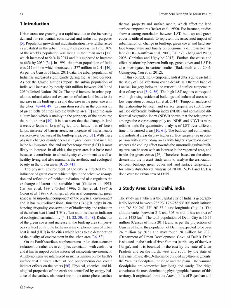
By all three methods, i.e. spectral radiance model (SRM),the mono-window algorithm (MWA) and split window algo-rithm (SWA), it is seen that LST is highest over built-up andopen land and lowest over vegetation and water bodies. Tocompare the change in LST, three methods are used, i.e.spectral radiance model and mono-window algorithm for2003, 2010 and 2017, whereas the split window algorithmis used only for 2017 Landsat 8 data. This is because thesplit window can be used only for those satellite datawhich have two thermal bands like in Landsat 8 (band 10and 11) both are thermal bands [12] whereas in Landsat 5

& 7, there is only one thermal band, i.e. band 6. All thethree models used in the study, i.e. SRM, MWA and SWA,show an increase in LST between 2003 and 2017. In 2003,LST ranged from 21.43 to 43.91 °C (MWA), and in 2017,LST ranged from 27.78 to 44.23 °C (MWA). According tothe split window algorithm maximum, LST in 2017 is45.22 °C. So, from the analysis of LST data, it can be saidthat in Delhi there is a slight increase in the maximumtemperature, i.e. about 1.5 to 2 °C. The highest LST in2003 is observed in southern and southwestern parts ofthe study area. In 2010, the highest LST and NDBI valuesare observed in western and northern parts of the state. In2017, the value of LST is highest recorded around theinternational airport near Palam in the southern part ofthe district. There are small patches of high LST value innorthern and eastern parts of the state too (Fig. 5).

Land Surface Temperature of NCT of Delhi

Fig. 5 LST image of NCT of Delhi, 2003–2017

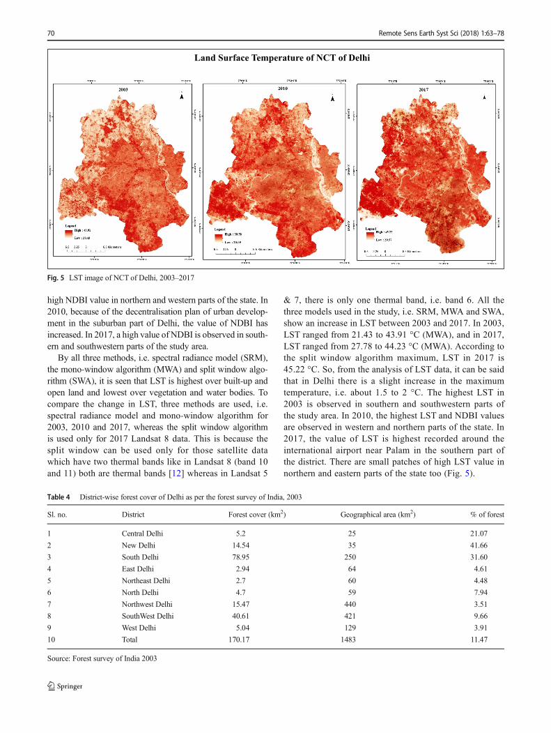
Table 4 District-wise forest cover of Delhi as per the forest survey of India, 2003

Sl. no. District Forest cover (km2) Geographical area (km2) % of forest

1 Central Delhi 5.2 25 21.07

2 New Delhi 14.54 35 41.66

3 South Delhi 78.95 250 31.60

4 East Delhi 2.94 64 4.61

5 Northeast Delhi 2.7 60 4.48

6 North Delhi 4.7 59 7.94

7 Northwest Delhi 15.47 440 3.51

8 SouthWest Delhi 40.61 421 9.66

9 West Delhi 5.04 129 3.91

10 Total 170.17 1483 11.47

Source: Forest survey of India 2003

70 Remote Sens Earth Syst Sci (2018) 1:63–78

As per the report of Forest Survey of India 2016, the areaunder vegetation in Delhi is about 10.20% of the total areaDelhi. The district-wise distribution of vegetation is highest inNew Delhi district (41.66%) followed by South Delhi district(31.60%) in 2003 (Table 3). The area under vegetation is alsohighest in 2015 in New Delhi district (49.29%) followed bySouth Delhi (32.86) (Table 4).

District-wise comparative analysis of NDVI, NDBI andLST on a temporal basis has been done where the averagevalue of NDVI, NDBI and LST is used for analysis. The studyshows that maximum value of NDVI is South Delhi district,i.e. 0.43, and minimum in New Delhi district, i.e. 0.31 in 2003(Table 6). The standard deviation of the NDVI is less than 0.23in the study area which shows that an average value of NDVIis close to the mean of NDVI. It means that there is almosteven distribution of vegetation all over Delhi.

The built-up density of each district is shown with the helpof distribution of NDBI value in all nine districts of Delhi. Thestudy shows that in 2003, NDBI is highest in northwest Delhi

district, i.e. 0.37, and lowest in northeast Delhi district, i.e.0.18. Land surface temperature is also calculated district-wise to show the distribution of surface temperature in all ninedistricts of Delhi. In 2003, the average land surface tempera-ture is highest in northwest Delhi district, i.e. 35.97 °C, andlowest in east Delhi district, i.e. 32.60 °C (MWA). It has beenslightly difficult to establish the relationship between NDVI,NDBI and LST in 2003. It is not clear from these data whethera change in land use/land cover results in a change in landsurface temperature in 2003.

In 2010, because of various developmental activities inDelhi, there is a decline in vegetation and an increase in den-sity of built-up. The study shows that the mean of NDVI ishighest in New Delhi district, i.e. 0.21, and lowest in north-west Delhi district, i.e. 0.11 (Table 7). It is further seen that theNewDelhi district has the lowest vegetation in 2003 (Table 4),but in 2010, the New Delhi district has the highest intensity ofvegetation (Table 7). This change in vegetation is mainly be-cause of different aforestation programmes that were started

Table 5 District-wise forest cover of Delhi as per the India State of Forest Report 2015

Sl. no. District Forest cover (km2) Geographical area (km2) % of forest

1 Central Delhi 5.14 25 20.56

2 New Delhi 17.25 35 49.29

3 South Delhi 82.14 250 32.86

4 East Delhi 3.28 64 5.13

5 Northeast Delhi 3.97 60 6.62

6 North Delhi 4.53 59 7.68

7 Northwest Delhi 17.04 440 3.87

8 Southwest Delhi 48.60 421 11.54

9 West Delhi 6.82 129 5.29

10 Total 178.77 1483 12.73

Source: Forest Department, Gov. of Delhi 2015

Table 6 District-level comparison of NDVI, NDBI and LST, 2003

S no. Districts NDVI NDBI LST(spectral radiance model)

LST(mono window algorithm)

Min Max Mean S.D Min Max Mean S.D Min Max Mean S.D Min Max Mean S.D

1 Central Delhi − 0.35 0.32 − 0.21 0.20 − 0.49 0.35 0.00 0.09 22.5 42.9 35.07 1.72 22.64 41.54 33.95 1.09

2 East Delhi − 0.36 0.35 − 0.34 0.19 − 0.45 0.25 − 0.19 0.14 21.32 41.6 34.18 2.25 20.42 41.54 32.60 1.31

3 New Delhi −0.35 0.31 − 0.41 0.19 − 0.44 0.26 − 0.03 0.14 22.70 42.9 34.17 1.73 20.43 39.61 33.11 1.16

4 North Delhi − 0.5 0.41 − 0.17 0.18 − 0.51 0.23 − 0.01 0.10 23.62 43.2 34.51 2.98 22.42 40.10 33.53 2.07

5 Northeast Delhi − 0.4 0.41 − 0.36 0.12 − 0.49 0.18 − 0.06 0.08 24.12 43.7 35.64 1.82 23.48 39.13 33.91 1.07

6 Northwest Delhi − 0.52 0.41 − 0.11 0.02 − 0.6 0.37 0.03 0.10 25.91 47.9 37.73 3.08 25.42 45.06 35.97 2.34

7 South Delhi −0.46 0.43 − 0.15 0.12 − 0.48 0.34 − 0.18 0.19 23.62 44.0 36.03 2.86 22.09 43.92 34.05 1.64

8 Southwest Delhi − 0.47 0.41 − 0.08 0.07 − 0.62 0.24 − 0.01 0.11 23.6 44.13 36.34 3.27 22.42 42.54 33.40 2.13

9 West Delhi − 0.38 0.32 − 0.07 0.23 − 0.64 0.34 − 0.09 0.17 25.9 43.1 36.26 2.42 24.95 41.54 33.42 1.61

NCT of Delhi − 0.52 0.43 − 0.17 0.11 − 0.64 0.36 − 0.08 0.17 23.40 44.01 35.87 3.29 21.43 43.91 33.31 1.60

Remote Sens Earth Syst Sci (2018) 1:63–78 71

by the Government of NCT of Delhi. Programmes like GreenDelhi Action Plan were started since 1997 by the forest de-partment of Delhi. As per the Delhi Development Master Plan2001, 8422 ha of land was earmarked for parks green(Department of Forest & Environment 2006).

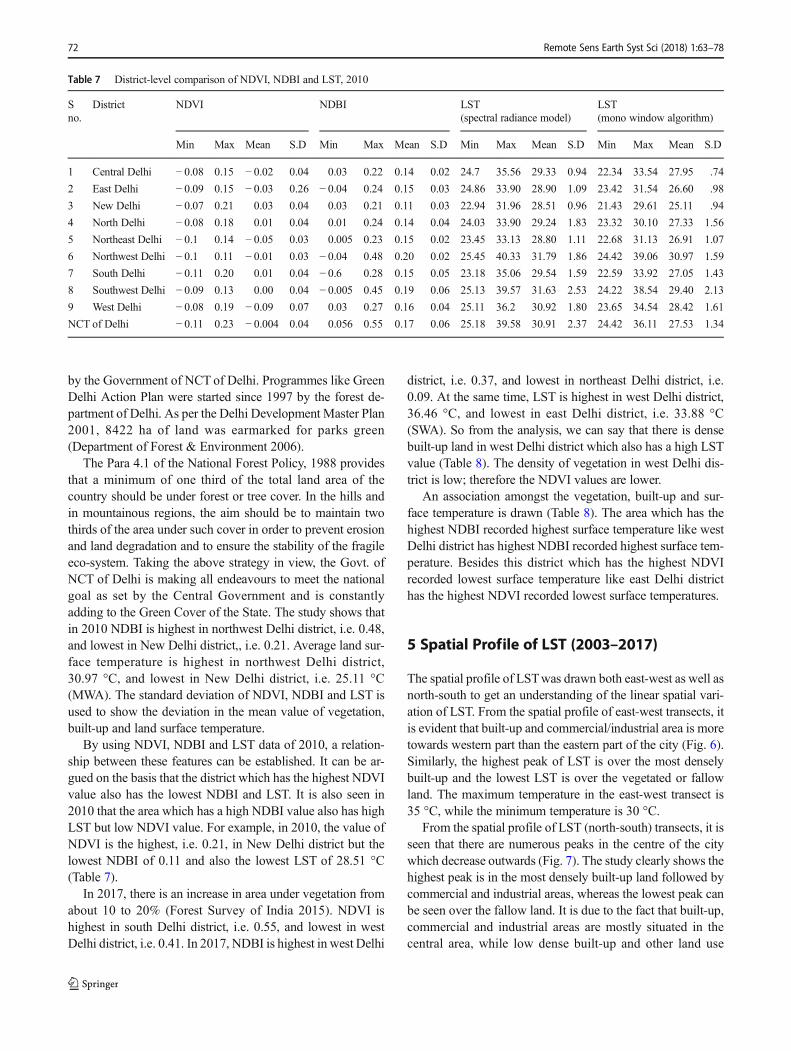
The Para 4.1 of the National Forest Policy, 1988 providesthat a minimum of one third of the total land area of thecountry should be under forest or tree cover. In the hills andin mountainous regions, the aim should be to maintain twothirds of the area under such cover in order to prevent erosionand land degradation and to ensure the stability of the fragileeco-system. Taking the above strategy in view, the Govt. ofNCT of Delhi is making all endeavours to meet the nationalgoal as set by the Central Government and is constantlyadding to the Green Cover of the State. The study shows thatin 2010 NDBI is highest in northwest Delhi district, i.e. 0.48,and lowest in New Delhi district,, i.e. 0.21. Average land sur-face temperature is highest in northwest Delhi district,30.97 °C, and lowest in New Delhi district, i.e. 25.11 °C(MWA). The standard deviation of NDVI, NDBI and LST isused to show the deviation in the mean value of vegetation,built-up and land surface temperature.

By using NDVI, NDBI and LST data of 2010, a relation-ship between these features can be established. It can be ar-gued on the basis that the district which has the highest NDVIvalue also has the lowest NDBI and LST. It is also seen in2010 that the area which has a high NDBI value also has highLST but low NDVI value. For example, in 2010, the value ofNDVI is the highest, i.e. 0.21, in New Delhi district but thelowest NDBI of 0.11 and also the lowest LST of 28.51 °C(Table 7).

In 2017, there is an increase in area under vegetation fromabout 10 to 20% (Forest Survey of India 2015). NDVI ishighest in south Delhi district, i.e. 0.55, and lowest in westDelhi district, i.e. 0.41. In 2017, NDBI is highest in west Delhi

district, i.e. 0.37, and lowest in northeast Delhi district, i.e.0.09. At the same time, LST is highest in west Delhi district,36.46 °C, and lowest in east Delhi district, i.e. 33.88 °C(SWA). So from the analysis, we can say that there is densebuilt-up land in west Delhi district which also has a high LSTvalue (Table 8). The density of vegetation in west Delhi dis-trict is low; therefore the NDVI values are lower.

An association amongst the vegetation, built-up and sur-face temperature is drawn (Table 8). The area which has thehighest NDBI recorded highest surface temperature like westDelhi district has highest NDBI recorded highest surface tem-perature. Besides this district which has the highest NDVIrecorded lowest surface temperature like east Delhi districthas the highest NDVI recorded lowest surface temperatures.

5 Spatial Profile of LST (2003–2017)

The spatial profile of LSTwas drawn both east-west as well asnorth-south to get an understanding of the linear spatial vari-ation of LST. From the spatial profile of east-west transects, itis evident that built-up and commercial/industrial area is moretowards western part than the eastern part of the city (Fig. 6).Similarly, the highest peak of LST is over the most denselybuilt-up and the lowest LST is over the vegetated or fallowland. The maximum temperature in the east-west transect is35 °C, while the minimum temperature is 30 °C.

From the spatial profile of LST (north-south) transects, it isseen that there are numerous peaks in the centre of the citywhich decrease outwards (Fig. 7). The study clearly shows thehighest peak is in the most densely built-up land followed bycommercial and industrial areas, whereas the lowest peak canbe seen over the fallow land. It is due to the fact that built-up,commercial and industrial areas are mostly situated in thecentral area, while low dense built-up and other land use

Table 7 District-level comparison of NDVI, NDBI and LST, 2010

Sno.

District NDVI NDBI LST(spectral radiance model)

LST(mono window algorithm)

Min Max Mean S.D Min Max Mean S.D Min Max Mean S.D Min Max Mean S.D

1 Central Delhi − 0.08 0.15 − 0.02 0.04 0.03 0.22 0.14 0.02 24.7 35.56 29.33 0.94 22.34 33.54 27.95 .74

2 East Delhi − 0.09 0.15 − 0.03 0.26 − 0.04 0.24 0.15 0.03 24.86 33.90 28.90 1.09 23.42 31.54 26.60 .98

3 New Delhi − 0.07 0.21 0.03 0.04 0.03 0.21 0.11 0.03 22.94 31.96 28.51 0.96 21.43 29.61 25.11 .94

4 North Delhi − 0.08 0.18 0.01 0.04 0.01 0.24 0.14 0.04 24.03 33.90 29.24 1.83 23.32 30.10 27.33 1.56

5 Northeast Delhi − 0.1 0.14 − 0.05 0.03 0.005 0.23 0.15 0.02 23.45 33.13 28.80 1.11 22.68 31.13 26.91 1.07

6 Northwest Delhi − 0.1 0.11 − 0.01 0.03 − 0.04 0.48 0.20 0.02 25.45 40.33 31.79 1.86 24.42 39.06 30.97 1.59

7 South Delhi − 0.11 0.20 0.01 0.04 − 0.6 0.28 0.15 0.05 23.18 35.06 29.54 1.59 22.59 33.92 27.05 1.43

8 Southwest Delhi − 0.09 0.13 0.00 0.04 − 0.005 0.45 0.19 0.06 25.13 39.57 31.63 2.53 24.22 38.54 29.40 2.13

9 West Delhi − 0.08 0.19 − 0.09 0.07 0.03 0.27 0.16 0.04 25.11 36.2 30.92 1.80 23.65 34.54 28.42 1.61

NCT of Delhi − 0.11 0.23 − 0.004 0.04 0.056 0.55 0.17 0.06 25.18 39.58 30.91 2.37 24.42 36.11 27.53 1.34

72 Remote Sens Earth Syst Sci (2018) 1:63–78

classes are mainly away from the centre. The spatial profile ofthe north-south transect has a very high thermal gradient incomparison to low thermal gradient along the east-west tran-sect. It is because more built-up land is towards west from thecentre of the city than north to south. The maximum andminimum temperatures along the north-south transect are42 °C and 32 °C. The spatial pattern of the land use/land coverclasses is quite useful to understand the urban heat island(UHI) pockets. It is inferred that the distribution of land use/land cover favours the development of UHI not only as adifference in temperature between the city centre and its pe-riphery but also amongst low dense built-up and the highdense built-up area in the entire city.

6 Discussion

There is no universal method which can accurately retrieveLSTs from all satellite TIR data because various LST retrievalmethods were proposed for use under different conditionswith different assumptions. Split window algorithms (SWA)is simple, effective and generally suitable for most sensors, soin most of the research based on LST, it is used for the LSTestimation. Root mean square error (RMSE) of SWA algo-rithm is low as more input parameters are explicitly included[51]. To determine which is the most capable of generating aconsistent LST climate data record RMSE of the differentalgorithm used for estimation of LST is calculated. The resultsshowed that the SWalgorithms that depend on both the meanand the difference of channel emissivity are the most accurateand stable over. However, the use of both the mean and thedifference of channel emissivity may be too sensitive to theemissivity uncertainty and should not be used in operationalpractice [60]. So in the present study, to decide which algo-rithm of LSTestimation is more accurate, the RMSE of LST iscalculated for 2017 because for 2017 LST estimation all thethree algorithms, i.e. SRM, MWA and SWA, have been used.It is observed that MWA gives the most accurate result in thestudy because the RMSE of MWA is the lowest (0.71 °C)amongst the three algorithms used in the study. RMSE ofSWA and SRM are 0.98 °C and 1.30 °C respectively.

The land surface temperature of any area is governed byphysical conditions, i.e. topography, land use and vegetation,of the city/urban areas. Distribution of vegetation, built-up,open land, water bodies and other features determines thesurface temperature [10]. Vegetation and water bodies act asa temperature regulator, so the area which has a high densityof vegetation and water bodies are comparatively cooler thanother areas which have low vegetation and water features. Inthis study, correlation is drawn amongst LST, NDBI andNDVI using Pearson correlation technique in SPSS softwareto show the relationship between LST, NDBI and NDVI at thedistrict level. It is seen that in 2003, 2010 and 2017 there is aTa

ble8

District-levelcom

parisonof

NDVI,NDBIandLST

,2017

Sno.

District

NDVI

NDBI

LST

(spectralradiancemodel)

LST

(monowindowalgorithm)

LST

(splitwindowalgorithm)

Min

Max

Mean

S.D

Min

Max

Mean

S.D

Min

Max

Mean

S.D

Min

Max

Mean

S.D

Min

Max

Mean

S.D

1CentralDelhi

−0.02

0.44

0.12

0.09

−0.22

0.12

−0.03

0.05

31.38

39.66

34.81

0.81

28.96

39.05

33.21

1.05

33.20

41.25

36.31

1.09

2EastD

elhi

−0.03

0.50

0.26

0.19

−0.38

0.24

−0.02

0.04

26.43

39.19

33.14

1.42

26.88

39.17

31.88

1.20

31.40

42.07

33.88

1.07

3New

Delhi

−0.01

0.47

0.20

0.07

−0.27

0.09

−0.08

0.09

29.87

39.46

33.29

0.82

28.66

38.03

32.59

1.27

32.67

40.43

34.01

1.02

4North

Delhi

0.08

0.53

0.23

0.14

−0.34

0.12

−0.07

0.05

26.68

40.29

34.25

1.76

26.51

39.93

32.06

1.63

30.77

42.37

35.67

1.35

5NortheastDelhi

−0.001

0.41

0.08

0.74

−0.27

0.09

−0.06

0.06

31.46

40.19

35.81

1.02

29.12

39.03

33.53

0.88

33.00

43.29

35.79

1.12

6NorthwestD

elhi

−0.09

0.52

0.14

0.07

−0.37

0.30

−0.04

0.06

27.26

42.39

35.02

1.82

26.73

42.17

32.39

2.18

30.29

42.76

36.02

1.08

7So

uthDelhi

−0.09

0.55

0.17

0.08

−0.42

0.19

−0.03

0.07

26.32

40.29

33.72

1.23

25.97

40.05

32.82

1.40

30.29

41.23

34.40

1.07

8So

uthw

estD

elhi

−0.05

0.52

0.16

0.09

−0.42

0.22

−0.14

0.03

26.69

44.19

33.99

1.42

26.02

43.17

33.41

2.33

30.29

45.67

35.43

1.16

9WestD

elhi

−0.06

0.40

0.12

0.07

−0.38

0.37

−0.01

0.05

29.46

44.82

35.97

1.26

27.22

44.31

33.73

1.41

30.56

46.47

36.46

1.05

NCTof

Delhi

−0.09

0.55

0.15

0.08

−0.42

0.35

−0.04

0.06

28.51

45.19

36.51

1.29

27.78

44.23

33.70

1.48

31.39

45.22

37.55

1.09

Remote Sens Earth Syst Sci (2018) 1:63–78 73

positive correlation between LST and NDBI whereas the neg-ative correlation between LSTand NDVI is observed. It is alsoseen that NDVI is negatively correlated with NDBI. There is achange in the degree of correlation amongst the LST, NDVIand NDBI. In 2003, there is a low degree of positive correla-tion between NDBI and LST (r2 = 0.383) Table 8 and mediumdegree of negative correlation between NDVI and LST (r2 =− 0.483). In 2010 and 2017, the correlation between LST andNDBI becomes stronger where r2 = 0.860 and 0.563 respec-tively (Tables 9, 10, 11).

A scatter plot is also drawn to show the correlation amongstthe LST, NDBI and NDVI because it is easy to understand thepictorial representation of correlation with the help of a scatterplot. The scatter plot of NDBI and LST shows the direct rela-tionship between LST and NDBI, indirect relationship be-tween LST and NDVI, and NDVI and NDBI in 2003

(Fig. 8a), 2010 (Fig. 8b) and 2017 (Fig. 8c). A positive corre-lation between LST and NDBI means that the area which hashigh NDBI value has high LST value and also an increase inNDBI causes an increase in LST. The negative correlationbetween LST and NDVI means an area which has lowNDVI has high LST and vice versa and decrease in NDVIcauses an increase in LST.

Different land use/land cover classes have different valuesof LST, NDVI and NDBI [62]. Areas with vegetation andwater body have lower temperature as compared to the built-up areas (Joshi and Bhatt 2012). LST and NDVI are posi-tively correlated during winter and negatively correlated dur-ing warm seasons [52]. LST and NDVI are positively corre-lated during winter and negatively correlated during warmseasons [52]. In this study, NDVI and LST were found to benegatively correlated. Vegetation has cooling effects on land

Fig. 6 East-west transects ofNCT of Delhi, 2017

Fig. 7 North-south transects ofNCT of Delhi, 2017

Table 9 Correlation between LST, NDBI and NDVI, 2003

2003 LST NDBI NDVI

LST Pearson correlation 1.0 0.383** − 0.483**

Sig. (2-tailed) – 0.000 0.000

N 310 310 310

NDBI Pearson correlation 0.383** 1.0 − 0.316**

Sig. (2-tailed) 0.000 – 0.000

N 310 310 310

NDVI Pearson correlation − 0.483** − 0.316** 1.0

Sig. (2-tailed) 0.000 0.000 –

N 310 310 310

**Correlation is significant at the 0.01 level (2-tailed)

Table 10 Correlation between LST, NDBI and NDVI, 2010

2010 LST NDBI NDVI

LST Pearson correlation 1.0 0.860** − 0.473**

Sig. (2-tailed) – 0.000 0.000

N 310 310 310

NDBI Pearson correlation 0.860** 1.0 − 0.553**

Sig. (2-tailed) 0.000 – 0.000

N 310 310 310

NDVI Pearson correlation −0.473** −0.553** 1.0

Sig. (2-tailed) 0.000 0.000 –

N 310 310 310

**Correlation is significant at the 0.01 level (2-tailed)

74 Remote Sens Earth Syst Sci (2018) 1:63–78

surface temperature ([24]; Xiao and Weng, 2007; [61]).Weng et al., [57] found LST was positively correlated withimpervious surface fraction but negatively correlated withgreen vegetation fraction. Li et al. [32] found there was astrong linear relationship between LST and NDBI, whereasthe relationship between LST and NDVI was much lessstrong and varies by season.

7 Conclusion

Delhi as a capital city of India attracts a large number of thepopulation every day for the want of education, employment,better infrastructure, better basic facilities and amenities etc.So over the period of time, the city gets crowded day by day.This will lead to an increase in built-up area for residential,commercial and industrial purposes. This will result in signif-icant loss of agricultural land, scrub land and forested land andgain in the high dense built-up land. Further, because of rapidurbanisation in NCT of Delhi, agricultural land also getscommercialised so farmers sell their land to the constructioncompanies in the greed of high profits. The study shows thatthere is continuous change in the distribution of vegetationand built-up land because of rapid urbanisation which resultsin the change in land use pattern. This leads to an increase inland surface temperature leading to the phenomena of urbanheat island (UHI) effect due to the clearing of vegetation forconstruction of residential complexes and commercial andindustrial centres.

The study has nicely demonstrated the use of Landsat 5, 7and 8 satellite data series to derive LST, NDBI and NDVI to

Table 11 Correlation between LST, NDBI and NDVI, 2017

2017 LST NDBI NDVI

LST Pearson correlation 1.0 0.563** − 0.494**

Sig. (2-tailed) – 0.000 0.000

N 310 310 310

NDBI Pearson correlation 0.563** 1.0 − 0.578**

Sig. (2-tailed) 0.000 – 0.000

N 310 310 310

NDVI Pearson correlation − 0.494** − 0.578** 1.0

Sig. (2-tailed) 0.000 0.000 –

N 310 310 310

**Correlation is significant at the 0.01 level (2-tailed)

-0.6

-0.4

-0.2

0

0.2

25 35 45

ND

BI

LST

Relationship between LST & NDBI, 2003

-0.6

-0.4

-0.2

0

0.2

0.4

25 35 45

ND

VI

LST

Relationship between LST & NDVI, 2003

-0.6

-0.4

-0.2

0

0.2

0.4

-0.5 0 0.5

ND

VI

NDBI

Relationship between NDBI & NDVI, 2003

0

0.05

0.1

0.15

0.2

0.25

0.3

25 30 35 40

ND

BI

LST

Relationship between LST & NDBI, 2010

-0.1

-0.05

0

0.05

0.1

0.15

25 30 35 40

ND

VI

LST

Relationship between LST & NDVI, 2010

-0.1

-0.05

0

0.05

0.1

0.15

0 0.1 0.2 0.3

ND

VI

NDBI

Relationship between NDBI & NDVI, 2010

-0.3

-0.2

-0.1

0

0.1

25 30 35 40

ND

BI

LST

Relationship between LST & NDBI, 2017

-0.1

0

0.1

0.2

0.3

0.4

25 30 35 40

ND

VI

LST

Relationship between LST & NDVI, 2017

-0.1

0

0.1

0.2

0.3

0.4

-0.4 -0.2 0 0.2

ND

VI

NDBI

Relationship between NDBI & NDVI, 2017

(a)

(b)

(c)

Fig. 8 Relationships between LST, NDBI and NDVI (2003, 2010 and 2017)

Remote Sens Earth Syst Sci (2018) 1:63–78 75

understand the urban environmental condition and also to drawout the relationships of LSTwith built-up and green cover overurban Delhi. In the absence of detailed meteorological data,Landsat satellite data of thermal sensor serve as an importanttool to draw out land surface temperature. It is seen in the studythat mono-window algorithm (MWA) and split window algo-rithm (SWA) give a better result than spectral radiance model.This is because in MWA and SWA, vegetation correction andwater vapour correction are applied. But MWA gives the mostaccurate result in this study since RMSE of MWA is the lowest(0.71 °C) amongst the three algorithms used in the study.Temporal analysis of land surface temperature by all the threealgorithms shows the increase in land surface temperature ofDelhi between 2003 and 2017. In 2003 the range of land sur-face temperature was 21.43 °C to 41.91 °C (MWA) whereas in2017 it increased to 31.39 °C to 45.22 °C (SWA).

The extracted data LST, NDBI and NDVI are nicelyused to the relationship amongst LST, NDBI and NDVI.It is seen that on an average area under forest in NCT ofDelhi in 2003 was 11.47% which slightly increased to12.73% in 2015. At district level, the area under forest ishighest, 41.66%, in New Delhi district in 2003 which in-creased to 49.29% in 2015 mainly because of variousaforestation programmes and management activities byDepartment of Forest, Government of Delhi. The studyshows that NDVI and LST are negatively correlated witheach other (r2 = − 0.494 in 2017) because vegetation has acooling effect on the surface temperature and NDBI andLST is positively correlated with each other (r2 = − 0.563in 2017). The district having low NDVI shows high LSTand vice versa, while the region having high NDBI showshigh LST. So, the present study shows the significant rela-tionship between the abundance of vegetation and low sur-face temperature as well as between an abundance of built-up with high surface temperature.

Acknowledgements The authors thank the United States GeologicalSurvey (USGS) for making available Landsat 5, Landsat 7 and Landsat8 satellite images which were downloaded from the Earth Explorer forthis study. The authors also sincerely wish to thank the learned reviewersfor their valuable comment which have greatly enhanced the paper.

Publisher’s note Springer Nature remains neutral with regard to jurisdic-tional claims in published maps and institutional affiliations.

References

1. Badarinath KVS, Kiran Chand TR, Madhavilatha K,Raghavaswamy V (2005) Studies on urban heat islands usingenvisat AATSR data. J Indian Soc Remote Sens 33(4):495–501

2. Becker F, Li Z-L (1990) Toward a local split-window method overland surface. Int J Remote Sens 11(3):369–393. https://doi.org/10.1080/01431169008955028

3. Bindi M, Brandani G, Dessì A, Dibari C, Ferrise R, Moriondo M,Trombi G (2009) Impact of Climate Change on Agricultural andNatural Ecosystems. Am J Environ Sci 5(5):633–638

4. Bolund P, Hunhammar S (1999) Ecosystem services in urban areas.Ecol Econ 29:293–301

5. Buyadi S, MohdW, Misni A (2013) Impact of land use changes onthe surface temperature distribution of area surrounding theNational Botanic Garden, Shah Alam. Procedia Soc Behav Sci101:516–525

6. Carlson TN, Gillies RR, Perry EM (1994) Amethod to make use ofthermal infrared temperature and NDVI measurements to infer sur-face soil water content and fractional vegetation cover. RemoteSens Rev 9(1-2):161–173

7. Chadchan J, Shankar R (2012) An analysis of urban growth trendsin the post-economic reforms period in India. Int J Sustain BuiltEnviron 1(1):36–49

8. Chandramouli C, General R (2011) Census of India 2011.Provisional Population Totals. Government of India, New Delhi

9. Chen YH, Wang J, Li XB (2002) A study on urban thermal field insummer based on satellite remote sensing. Remote Sens LandResour 4(1)

10. Chen XL, Zhao HM, Li PX, Yin ZY (2006) Remote sensing image-based analysis of the relationship between urban heat island andland use/cover changes. Remote Sens Environ 104(2):133–146

11. Colding J (2007) Ecological land-use complementation for buildingresilience in urban ecosystems. Landsc Urban Plan 81:46–55

12. Du C, Ren H, Qin Q, Meng J, Zhao S (2015) A practical split-window algorithm for estimating land surface temperature fromLandsat 8 data. Remote Sens:647–665

13. Dutta D, RahmamA,KunduA (2015) Growth of Dehradun city: anapplication of linear spectral unmixing (LSU) technique usingmulti-temporal Landsat satellite data sets, Remote SensingApplications: Society and Environment (RSASE), vol. 1, no 1.Elsevier Science Publication, Amsterdam, pp 98–111. https://doi.org/10.1016/j.rsase.2015.07.001

14. Elizabeth AW, Nelson D, Rahman A, StefanovWL, Roy SS (2008)Expert system classification of urban land use/cover for Delhi,India. Int J Remote Sens 29(15. Taylor & Francis Publisher,London):4405–4427

15. EssaW, Verbeiren B, Kwast JVD, Voorde TVD, Batelaan O (2012)Evaluation of the DisTrad thermal sharpening methodology forurban areas. Int J Appl Earth Obs Geoinf 19:163–172

16. Essa W, Kwast JVD, Verbeiren B, Batelaan O (2013) Downscalingof thermal images over urban areas using the land surfacetemperature–impervious percentage relationship. Int J Appl EarthObs Geoinf 23:95–108

17. FSI (Forest Survey of India). India state of forest report18. Forest Survey of India. State of Forest Report-2003. Forest Survey

of India; 200319. Forest Survey of India (2015) India state of forest report 2015.

Forest Survey of India20. Gallo KP, Tarpley JD, McNab AL, Karl TR (1995) Assessment of

urban heat islands: a satellite perspective. Atmos Res 37(1-3):37–43

21. Gao B-C (1996) NDWI—a normalized difference water index forremote sensing of vegetation liquid water from space. Remote SensEnviron 58(3):257–266

22. Gaston KJ, Warren PH, Thompson K, Smith RM (2005) Urbandomestic gardens (IV): the extent of the resource and its associatedfeatures. Biodivers Conserv 14:3327–3349

23. Gillies RR, Kustas WP, Humes KS (2010) A verification of the'triangle' method for obtaining surface soil water content and energyfluxes from remote measurements of the Normalized Difference

76 Remote Sens Earth Syst Sci (2018) 1:63–78

Vegetation Index (NDVI) and surface e. Int J Remote Sens 18(15):3145–3166

24. Goetz SJ (1997) Multi-sensor analysis of NDVI, surface tempera-ture and biophysical variables at a mixed grassland site. Int JRemote Sens 18(1):71–94

25. Gorgani SA, Panahi M, Rezaie F (2013) The relationship betweenNDVI and LST in the urban area of Mashhad, Iran. InternationalConference on Civil Engineering Architecture &Urban SustainableDevelopment, At Tabriz, Iran

26. Hang HT, Rahman A (2018) Characterization of thermal environ-ment over heterogeneous surface of National Capital Region(NCR), India using LANDSAT-8 sensor for regional planning stud-ies. Urban Climate:1–18. https://doi.org/10.1016/j.uclim.2018.01.001

27. Jiménez-Muñoz JC, Cristóbal J, Sobrino JA, Sòria G, Ninyerola M,Pons X (2009) Revision of the single-channel algorithm for landsurface temperature retrieval from Landsat thermal-infrared data.IEEE Trans Geosci Remote Sens 47(1):339–349

28. Joshi JP, Bhatt B (2012) Estimating temporal land surface temper-ature using remote sensing: A study of Vadodara urban area,Gujarat. Int J Geol Earth Environ Sci 2(1):123–130

29. Kaufmann RK, Zhou L, Myneni RB, Tucker CJ, Slayback D,Shabanov NV, Pinzon J (2003) The effect of vegetation on surfacetemperature: A statistical analysis of NDVI and climate data.Geophys Res Lett 30(22)

30. Kühn I, Klotz S (2006) Urbanization and homogenization—comparing the floras of urban and rural areas in Germany. BiolConserv 127:292–300

31. KumarKS, Bhaskar PU, Padmakumari K (2012) Estimation of landsurface temperature to study urban heat island effect using LandsatETM + IMAGE. Int J Eng Sci Technol 4(02):771–778

32. Li H, LiuQ, Zou J (2009) Relationships of LST toNDBI and NDVIin Changsha-Zhuzhou-Xiangtan area based on MODIS data. SciGeogr Sin 29(2):262–267

33. Li Z-L, Tang B-H, Wu H, Ren H, Yan G, Wan Z, Trigo IF, SobrinoJA (2013) Satellite-derived land surface temperature: Current statusand perspectives. Remote Sens Environ 131:14–37

34. Malik K (2014) Human development report 2014: Sustaining hu-man progress: Reducing vulnerabilities and building resilience.United Nations Development Programme, New York

35. Mallick J, Kant Y, Bharath BD (2008) Estimation of land surfacetemperature over Delhi using Landsat-7 ETM+. J Ind GeophysUnion 12(3):131–140

36. Mallick J, Rahman A, Singh CK (2013) Modeling urban heatislands in heterogeneous land surface and its correlation with im-pervious surface area by using night-time ASTER satellite data inhighly urbanizing city, Delhi- India, advances in space research,Elsevier Science Publication, vol 52, no. 4, pp 639–655. https://doi.org/10.1016/j.asr.2013.04.025

37. Nichol JE (1996) High-Resolution Surface Temperature PatternsRelated to Urban Morphology in a Tropical City: A Satellite-Based Study. J Appl Meteorol 35(1):135–146

38. Opeyemi A, Trina W (2014) Potential application of change inurban green space as an indicator of urban environmental qualitychange. Universal J Geosci 2:222–228

39. Owen TW, Carlson TN, Gillies RR (2010) An assessment of satel-lite remotely-sensed land cover parameters in quantitatively de-scribing the climatic effect of urbanization. Int J Remote Sens19(9):1663–1681

40. Pandey B, Seto KC (2015) Urbanization and agricultural land lossin India: comparing satellite estimates with census data. J EnvironManag 148:53–66

41. Pauleit S, Duhme F (2000) Assessing the environmental perfor-mance of landcover types for urban planning. Landsc Urban Plan52:1–20

42. RahmanA (2007) Application of remote sensing andGIS techniquefor urban environmental management and sustainable developmentof Delhi, India. In: Netzband M, Stefnow WL, Redman CL (eds)Applied remote sensing for urban planning, governance and sus-tainability. Springer-Verlag Publishes, Berlin, pp 165–197

43. Rahman A, Kumar S, Fazal S, Siddiqui MA (2012) Assessment ofland use/land cover change in the North-West District of Delhiusing remote sensing and GIS techniques. J Indian Soc RemoteSens 40(4):689–697

44. Rahman A, Khan J, Ali I, Khan TA, Alam SD (2013) Dynamics ofLand Use/Land Cover Changes in Ballia District, Using LandsatTM Data. J Remote Sens GIS 4(1):29–35

45. Ramachandra TV, UttamKK (2009) Land surface temperature withland cover dynamics: multi-resolution, spatiotemporal data analysisof Greater Bangalore. Int J Geoinform 5(3)

46. Rao P, Puntambekar DK (2014) Evaluating the Urban Green Spacebenefits and functions at macro, meso and micro level: case ofBhopal City. International Journal of Engineering Research &Technology (IJERT) IJERTIJERT ISSN: 2278–0181

47. Sachs JD (2012) From Millennium Development Goals toSustainable Development Goals. Lancet 379(9832):2206–2211

48. Senanayake IP, Welivitiya WDDP, Nadeeka PM (2013)Assessment of green space requirement and site analysis inColombo, Sri Lanka—a remote sensing and GIS approach. Int JSci Eng Res 4(12) ISSN 2229–5518

49. Shahmohamadi P, Che-Ani AI, Maulud KN, Tawil NM, AbdullahNA (2011) The impact of anthropogenic heat on formation of urbanheat island and energy consumption balance. Urban Stud Res 2011

50. Sobrino JA, Jiménez-Muñoz JC, Paolini L (2004) Land surfacetemperature retrieval from LANDSAT TM 5. Remote SensEnviron 90(4):434–440

51. Sòria G, Sobrino JA (2007) ENVISAT/AATSR derived land sur-face temperature over a heterogeneous region. Remote SensEnviron 111:409–422

52. Sun D, Kafatos M (2007) Note on the NDVI-LST relationship andthe use of temperature-related drought indices over North America.Journal of Geophysical research letters 34

53. Tongliga B, Xueming L, Jing Z, Yingjia Z, Shenzhen T (2016)Assessing the distribution of urban green spaces and its anisotropiccooling distance on urban heat island pattern in Baotou, China. Int JGeo-Inform 5(2):12

54. Towards Greener Delhi (2006) Department of Environment andForests, Government of National Capital Territory of Delhi, pp.1–18

55. Ukwattage NL, Dayawansa NDK (2012) Urban heat islands andthe energy demand: an analysis for Colombo City of Sri Lankausing thermal remote sensing data. Int J Remote Sens GIS 1(2):124–131

56. Weng Q (2001) A remote sensing-GIS evaluation of urban expan-sion and its impact on surface temperature in ZhujiangDelta, China.Int J Remote Sens 22(10):1999–2014

57. Weng Q, Lu D, Schubring J (2004) Estimation of land surfacetemperature-vegetation abundance relationship for urban heat is-land studies. Remote Sens Environ 89(4):467–483

58. You G, Zhang Y, Liu Y, Schaefer D, Gong H, Gao J, Lu Z, Song Q,Zhao J, Wu C, Yu L, Xie Y (2013) Investigation of temperature andaridity at different elevations of Mt. Ailao, SW China. Int JBiometeorol 57(3):487–492

Remote Sens Earth Syst Sci (2018) 1:63–78 77

59. Yu Y, Privette JL, Pinheiro AC (2008) Evaluation of split-windowland surface temperature algorithms for generating climate datarecords. IEEE Trans Geosci Remote Sens 46:179–192

60. Yu Y, Tarpley D, Privette JL, Goldberg MD, Rama MK, Raja M,Vinnikov KY (2009) Developing algorithm for operational GOES-R land surface temperature product. IEEE Trans Geosci RemoteSens 47:936–951

61. Yuan F, Bauer ME (2007) Comparison of impervious surface areaand normalized difference vegetation index as indicators of surfaceurban heat island effects in Landsat imagery. Remote Sens Environ106(3):375–386

62. Yue W, Xu J, Tan W, Xu L (2007) The relationship between landsurface temperature and NDVI with remote sensing: application toShanghai Landsat & ETM+ data. Int J Remote Sens (15):3205–3226

63. Zha Y, Gao J, Ni S (2003) Use of normalized difference built-upindex in automatically mapping urban areas from TM imagery. Int JRemote Sens 24(3):583–594

64. Zhang J, Wang Y (2008) Study of the Relationships between theSpatial Extent of Surface Urban Heat Islands and UrbanCharacteristic Factors Based on Landsat ETM+ Data. Sensors8(11):7453–7468

78 Remote Sens Earth Syst Sci (2018) 1:63–78