SOME ASPECTS OF NON-LINEAR OPTIMIZATION

A PROJECT REPORT

submitted by

SASMITA PATEL

for

the partial fulfilment for the award of the degree

of

Master of Science in Mathematics

under the supervision

of

PROF. ANIL KUMAR

DEPARTMENT OF MATHEMATICSNIT ROURKELA

ROURKELA– 769008

MAY 2014

1

Certificate

This is to certify that the project report entitled SOME ASPECTS OF NON-LINEAROPTIMIZATION submitted by SASMITA PATEL to the National Institute of Tech-nology Rourkela, Orissa for the partial fulfilment of requirements for the degree of masterof science in Mathematics is a bonafide record of review work carried out by her under mysupervision and guidance. The contents of this project, in full or in parts, have not beensubmitted to any other institute or university for the award of any degree or diploma.

May, 2014(Prof. Anil Kumar)

Department of MathematicsNIT Rourkela

2

ACKNOWLEDGEMENT

It is my pleasure to thank to the people, for whom this dissertation is possible. I spe-cially like to thank my guide Prof.Anil Kumar, for his keen guidance and encouragementduring the course of study and preparation of the final manuscript of this project. Iwould also like to thank the faculty members of Department of Mathematics for their co-operation. I heartily thank to my friends, who helped me during the preparation of thisproject. I thank the Director, National Institute of Technology Rourkela, for providingthe facilities to pursue my postgraduate degree. I thank all my classmates and friends formaking my stay memorable at National Institute of Technology Rourkela.

Finally, I also thank my parents for their constant inspiration. (Sasmita Patel)

3

ABSTRACT

We provide a concise introduction to some methods for solving nonlinear optimizationproblems. This dissertation includes a literature study of the formal theory necessary forunderstanding optimization and an investigation of the algorithms available for solving aspecial class of the non-linear programming problem, namely the quadratic programmingproblem. It was not the intention of this dissertation to discuss all possible algorithms forsolving the quadratic programming problem, therefore certain algorithms for convex andnon-convex quadratic programming problems . Some of the algorithms were selected arbi-trarily, because limited information was available comparing the efficiency of the variousalgorithms.

4

Contents

1 Introduction 6

2 Preliminaries 72.1 Local Optimal Point . . . . . . . . . . . . . . . . . . . . . . . . . . . . . . 72.2 Global Optimal Point . . . . . . . . . . . . . . . . . . . . . . . . . . . . . . 72.3 Convex Function . . . . . . . . . . . . . . . . . . . . . . . . . . . . . . . . 7

3 NON-LINEAR OPTIMIZATION 83.1 Introduction . . . . . . . . . . . . . . . . . . . . . . . . . . . . . . . . . . . 83.2 General Non-Linear Programming Problem . . . . . . . . . . . . . . . . . . 83.3 Unconstrained Optimization . . . . . . . . . . . . . . . . . . . . . . . . . . 93.4 Constrained Optimization . . . . . . . . . . . . . . . . . . . . . . . . . . . 10

3.4.1 Lagrange Multiplier Method . . . . . . . . . . . . . . . . . . . . . . 103.4.2 Kuhn-Tucker Condition . . . . . . . . . . . . . . . . . . . . . . . . 11

4 GRAPHICAL SOLUTION OF NLPP 13

5 QUADRATIC PROGRAMMING 155.1 Introduction . . . . . . . . . . . . . . . . . . . . . . . . . . . . . . . . . . . 155.2 General Quadratic Programming . . . . . . . . . . . . . . . . . . . . . . . 155.3 Wolfe’s Method . . . . . . . . . . . . . . . . . . . . . . . . . . . . . . . . . 165.4 Beale’s Method . . . . . . . . . . . . . . . . . . . . . . . . . . . . . . . . . 19

6 SEPARABLE PROGRAMMING 236.1 Introduction . . . . . . . . . . . . . . . . . . . . . . . . . . . . . . . . . . . 236.2 Separable Function . . . . . . . . . . . . . . . . . . . . . . . . . . . . . . . 236.3 Separable Programming Problem . . . . . . . . . . . . . . . . . . . . . . . 246.4 Reduction of separable programming problem to linear programming problem 246.5 Separable Programming Algorithm . . . . . . . . . . . . . . . . . . . . . . 25

5

CHAPTER 1

1 Introduction

The term ’non linear programming’ usually refers to the problem in which the objectivefunction becomes non-linear, or one or more of the constraint inequalities have non-linearor both.The solution of nonlinear optimization problems that is the minimization or max-imization of an objective function involving unknown parameters/variables in which thevariables may be restricted by constraints is one of the core components of computationalmathematics. Nature (and man) loves to optimize, and the world is far from linear.In Applied Mathematics, the eminent mathematician Gil Strange opines that optimiza-tion, along with the solution of systems of linear equations, and of (ordinary and partial)differential equations, is one of the three cornerstones of modern applied mathematics.

6

CHAPTER 2

2 Preliminaries

2.1 Local Optimal Point

A point x∗ is said to be a local optimal point, if there exist no point in the neighbourhoodof x∗ which is better than x∗. similarly a point x∗ is a local minimal point if no point inthe neighborhood has a function value smaller than f(x∗).

2.2 Global Optimal Point

A point x∗∗ is said to be a Global optimal point , if there is no point in the entire searchspace which is better than the point x∗∗. similarly a point x∗∗ is a Global minimal pointif no point in the entire search space has a function value smaller than f(x∗∗).

2.3 Convex Function

A function f(x) is said to be convex function over the region ′S ′. If for any two pointsx1, x2 ∈ S we have the function

f(λx1 + (1− λ)x2) ≤ λf(x1) + (1− λ)f(x2)

where 0 ≤ λ ≤ 1Strictly convex function means

f(λx1 + (1− λ)x2) < λf(x1) + (1− λ)f(x2)

where 0 ≤ λ ≤ 1

7

CHAPTER 3

3 NON-LINEAR OPTIMIZATION

3.1 Introduction

The Linear Programming Problem which can be review as to

maximize Z =n∑j=1

cjxj (1)

subject ton∑j=1

aijxj ≤ bi for i = 1, 2, ...,m (2)

and xj ≥ 0 for j = 1, 2, ..., n (3)

The term ’non linear programming’ usually refers to the problem in which the objectivefunction (1) becomes non-linear, or one or more of the constraint inequalities (2) havenon-linear or both.

3.2 General Non-Linear Programming Problem

The mathematical formulation of general non linear programming problem may be ex-pressed as follows:

max.(or min.)z=C(x1, x2, ..., xn) ,subject to the constraints:

a1(x1, x2, ..., xn){≤,= or ≥}b1a2(x1, x2, ..., xn){≤,= or ≥}b2a3(x1, x2, ..., xn){≤,= or ≥}b3

..............................am(x1, x2, ..., xn){≤,= or ≥}bm

and xj ≥ 0, j = 1, 2, ..., n

where either C(x1, x2, ..., xn) or some ai(x1, x2, ..., xn), i = 1, ...,m; or both are non-linear.In matrix notation,the general non-linear programming problem may be written as follows:

max.(or min.)z = C(X), subject to the constraints:ai(X){≤,= or,≥}bi, i = 1, 2, ...,m

and X ≥ 0,

where either C(X) or some ai(X) or both are non linear in X.

For Example:max.Z = 2x1 + 3x2subject to x1

2 + x22 ≤ 20, and x1, x2 ≥ 0

8

3.3 Unconstrained Optimization

We use to.

optimize f(x1, x2, ..., xn)

The extreme points from the solution∂f

∂x1= 0

∂f

∂x2= 0

...

∂f

∂xn= 0

For one Variable

∂2f

∂x2> 0 Then f is minimum.

∂2f

∂x2< 0 Then f is maximum.

∂2f

∂x2= 0 Then further investigation needed.

For two variable

rt− s2 > 0 Then the function is minimum.rt− s2 < 0 Then the function is maximum.rt− s2 = 0 Further investigation needed.

Where r =∂2f

∂x12, s =

∂2f

∂x1x2, t =

∂2f

∂x22For ’n’ Variable

Hessian Matrix

∂2f

∂x12∂2f

∂x1∂x2. . . . . . . . .

∂2f

∂x1∂xn

∂2f

∂x1∂x2

∂2f

∂x22. . . . . . . . .

∂2f

∂x2∂xn...

...∂2f

∂x1∂xn

∂2f

∂x2∂xn. . . . . . . . .

∂2f

∂xn2

det (H) > 0 at p1,f is attains minimum at p1.det (H) < 0 at p1,f is attains maximum at p1.

9

3.4 Constrained Optimization

optimizef(x1, x2, ..., xn)subject to gi(x1, x2, ..., xn) = 0, i = 1(1)mand xi ≥ 0 ∀iFor solving this we use Lagrange Multiplier Method and Kuhn-Tucker Condition.

3.4.1 Lagrange Multiplier Method

Here we discussed the optimization problem of continuous functions. The non-linear pro-gramming problem is composed of some differentiable objective function and equality sideconstraints, the optimization may be achieved by the use of Lagrange multipliers.A Lagrange multiplier measures the sensitivity of the optimal value of the objective func-tion to change in the given constraints bi in the problem.

Consider the problem of determining the global optimum of

Z = f(x1, x2, ..., xn)

subject to the constraints

gi (x1, x2, ..., xn) = bi , i = 1, 2, ...,m.

Let us first formulate the Lagrange function L defined by:

L(x1, ..., xn;λ1, ..., λm) = f(x1, ..., xn) + λ1g1(x1, ..., xn) + λ2g2(x1, ..., xn) + ...+ λmgm(x1, ..., xn)

whereλ1, λ2, ..., λm are called Lagrange Multiplier.For the stationary points

∂L

∂xj= 0 ,

∂L

∂λi= 0 ∀ j = 1(1)n ∀ i = 1(1)m

Solving the above equation to get stationary points.

Example:1

min.f(x1, x2) = x12 + x2

2

x1x2 = 1and x1, x2 ≥ 0solution: form lagrangian multiplier function

L(x1, x2, λ) = x12 + x2

2 + λ(x1x2 − 1)

for the stationary points

∂L

∂x1= 0⇒ 2x1 + λx2 = 0 (4)

∂L

∂x2= 0⇒ 2x2 + λx1 = 0 (5)

∂L

∂λ= 0⇒ x1x2 − 1 = 0 (6)

10

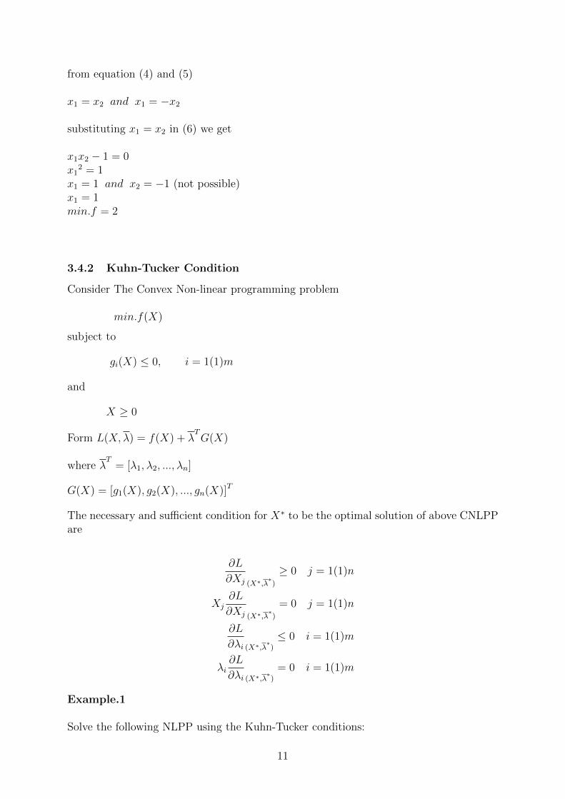
from equation (4) and (5)

x1 = x2 and x1 = −x2

substituting x1 = x2 in (6) we get

x1x2 − 1 = 0x1

2 = 1x1 = 1 and x2 = −1 (not possible)x1 = 1min.f = 2

3.4.2 Kuhn-Tucker Condition

Consider The Convex Non-linear programming problem

min.f(X)

subject to

gi(X) ≤ 0, i = 1(1)m

and

X ≥ 0

Form L(X,λ) = f(X) + λTG(X)

where λT

= [λ1, λ2, ..., λn]

G(X) = [g1(X), g2(X), ..., gn(X)]T

The necessary and sufficient condition for X∗ to be the optimal solution of above CNLPPare

∂L

∂Xj (X∗,λ∗)

≥ 0 j = 1(1)n

Xj∂L

∂Xj (X∗,λ∗)

= 0 j = 1(1)n

∂L

∂λi (X∗,λ∗)

≤ 0 i = 1(1)m

λi∂L

∂λi (X∗,λ∗)

= 0 i = 1(1)m

Example.1

Solve the following NLPP using the Kuhn-Tucker conditions:

11

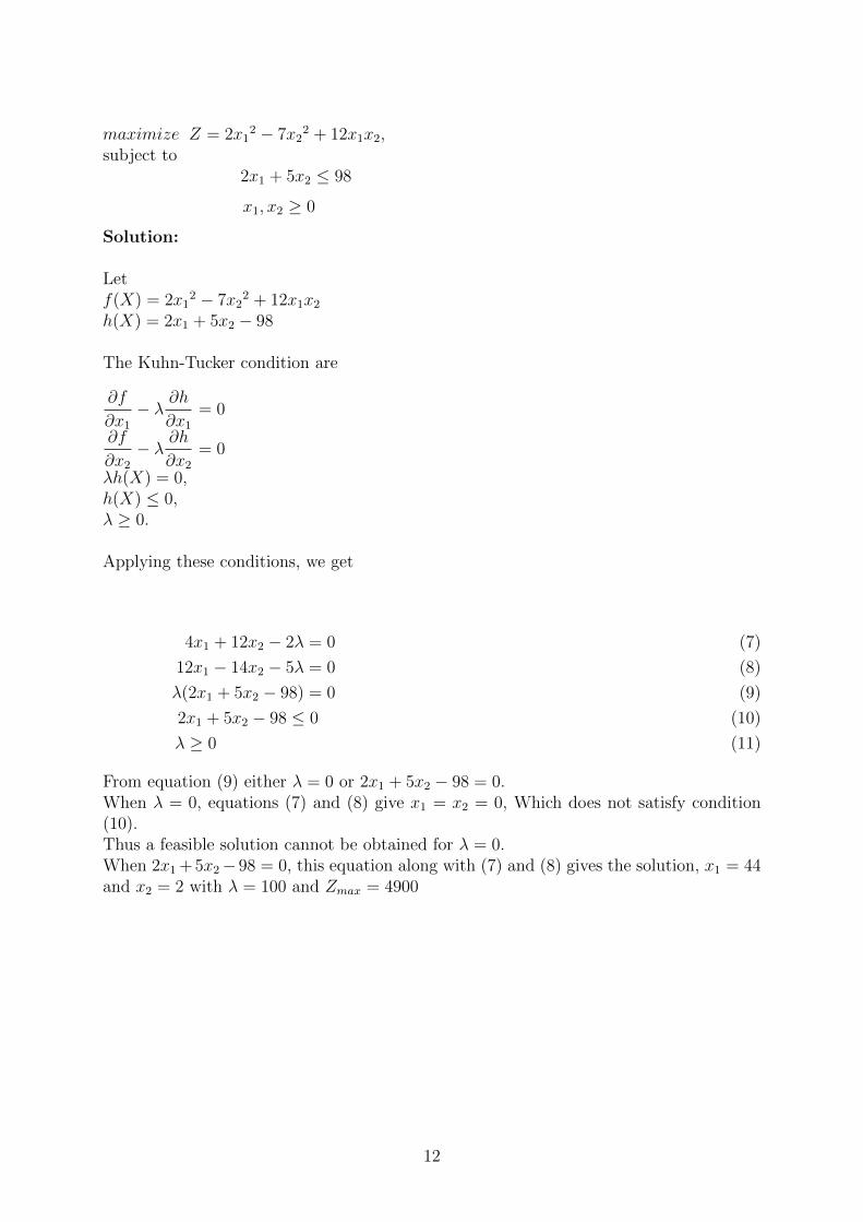
maximize Z = 2x12 − 7x2

2 + 12x1x2,subject to

2x1 + 5x2 ≤ 98

x1, x2 ≥ 0

Solution:

Letf(X) = 2x1

2 − 7x22 + 12x1x2

h(X) = 2x1 + 5x2 − 98

The Kuhn-Tucker condition are

∂f

∂x1− λ ∂h

∂x1= 0

∂f

∂x2− λ ∂h

∂x2= 0

λh(X) = 0,h(X) ≤ 0,λ ≥ 0.

Applying these conditions, we get

4x1 + 12x2 − 2λ = 0 (7)

12x1 − 14x2 − 5λ = 0 (8)

λ(2x1 + 5x2 − 98) = 0 (9)

2x1 + 5x2 − 98 ≤ 0 (10)

λ ≥ 0 (11)

From equation (9) either λ = 0 or 2x1 + 5x2 − 98 = 0.When λ = 0, equations (7) and (8) give x1 = x2 = 0, Which does not satisfy condition(10).Thus a feasible solution cannot be obtained for λ = 0.When 2x1 + 5x2−98 = 0, this equation along with (7) and (8) gives the solution, x1 = 44and x2 = 2 with λ = 100 and Zmax = 4900

12

CHAPTER 4

4 GRAPHICAL SOLUTION OF NLPP

In a linear programming problem, the optimal solution was usually obtained at one ofthe extreme points of the convex region generated by the constraints and the objectivefunction of the problem. But, it is not necessary to find the solution at a corner or edgeof the feasible region of non-linear programming problem.

example-1 :solve graphically the following problemmaximizez = 3x1 + 5x2subject tox1 ≤ 49x1

2 + 5x22 ≤ 216

and x1, x2 ≥ 0solution:x1 = 4

9x12+5x2

2 = 216 (1)

⇒ x12

216

9

+x2

2

216

5

= 1

it is a equation of ellipse let 3x1 + 5x2 = know differentiate the equation with respect to x1

3 + 5dx2dx1

= 0

13

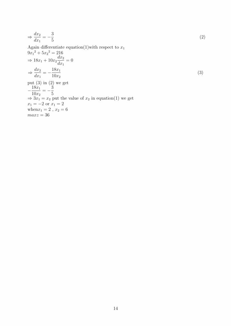
⇒ dx2dx1

= −3

5(2)

Again differentiate equation(1)with respect to x19x1

2 + 5x22 = 216

⇒ 18x1 + 10x2dx2dx1

= 0

⇒ dx2dx1

= −18x110x2

(3)

put (3) in (2) we get

−18x110x2

= −3

5⇒ 3x1 = x2 put the value of x2 in equation(1) we getx1 = −2 or x1 = 2whenx1 = 2 , x2 = 6maxz = 36

14

CHAPTER 5

5 QUADRATIC PROGRAMMING

5.1 Introduction

Quadratic programming problems are very similar to linear programming problems. Themain difference between the two is that our objective function is now a quadratic function(the constraints are still linear).Because of its many applications, quadratic programmingis often viewed as a discipline in and of itself. More importantly, though, it forms the basisof several general nonlinear programming algorithms. We begin this section by examiningthe Karush-Kuhn-Tucker conditions for the QP and see that they turn out to be a set oflinear equalities and complementarity constraints. Much like in separable programming,a modified version of the simplex algorithm can be used to find solutions.

Quadratic Form

A Homogeneous polynomial of degree two in any number of variables is called a Quadraticforms or an expression of the form

n∑i=1

n∑j=1

aijxixj

is called Quadratic form of n variable.

5.2 General Quadratic Programming

Definition. let xT and c ∈ Rn and, Q be a symmetric n× n real matrix. Then,

max f(X) = CX +1

2XTQX

subject to

AX ≤ b

andX ≥ 0

.where bT ∈ Rm and A be m × n real matrix is called a general quadratic programmingproblem.

The function XTQX defines a quadratic form with Q being a symmetric matrix. Thequadratic form XTQX is said to be positive definite if XTQX > 0 for X 6= 0 and positive-semi-definite if XTQX ≥ 0 for all X such that there is one X 6= 0 satisfying XTQX = 0.Similarly, XTQX is said to be negative definite and negative-semi-definite if −XTQX ispositive-definite and positive-semi-definite respectively. The function XTQX is assumedto be negative-definite in the maximization case, and positive definite in the minimizationcase.

15

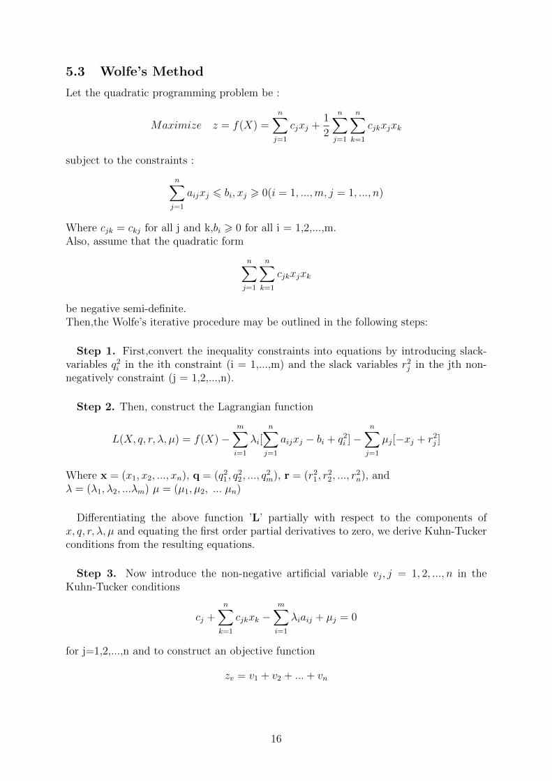
5.3 Wolfe’s Method

Let the quadratic programming problem be :

Maximize z = f(X) =n∑j=1

cjxj +1

2

n∑j=1

n∑k=1

cjkxjxk

subject to the constraints :

n∑j=1

aijxj 6 bi, xj > 0(i = 1, ...,m, j = 1, ..., n)

Where cjk = ckj for all j and k,bi > 0 for all i = 1,2,...,m.Also, assume that the quadratic form

n∑j=1

n∑k=1

cjkxjxk

be negative semi-definite.Then,the Wolfe’s iterative procedure may be outlined in the following steps:

Step 1. First,convert the inequality constraints into equations by introducing slack-variables q2i in the ith constraint (i = 1,...,m) and the slack variables r2j in the jth non-negatively constraint (j = 1,2,...,n).

Step 2. Then, construct the Lagrangian function

L(X, q, r, λ, µ) = f(X)−m∑i=1

λi[n∑j=1

aijxj − bi + q2i ]−n∑j=1

µj[−xj + r2j ]

Where x = (x1, x2, ..., xn), q = (q21, q22, ..., q

2m), r = (r21, r

22, ..., r

2n), and

λ = (λ1, λ2, ...λm) µ = (µ1, µ2, ... µn)

Differentiating the above function ’L’ partially with respect to the components ofx, q, r, λ, µ and equating the first order partial derivatives to zero, we derive Kuhn-Tuckerconditions from the resulting equations.

Step 3. Now introduce the non-negative artificial variable vj, j = 1, 2, ..., n in theKuhn-Tucker conditions

cj +n∑k=1

cjkxk −m∑i=1

λiaij + µj = 0

for j=1,2,...,n and to construct an objective function

zv = v1 + v2 + ...+ vn

16

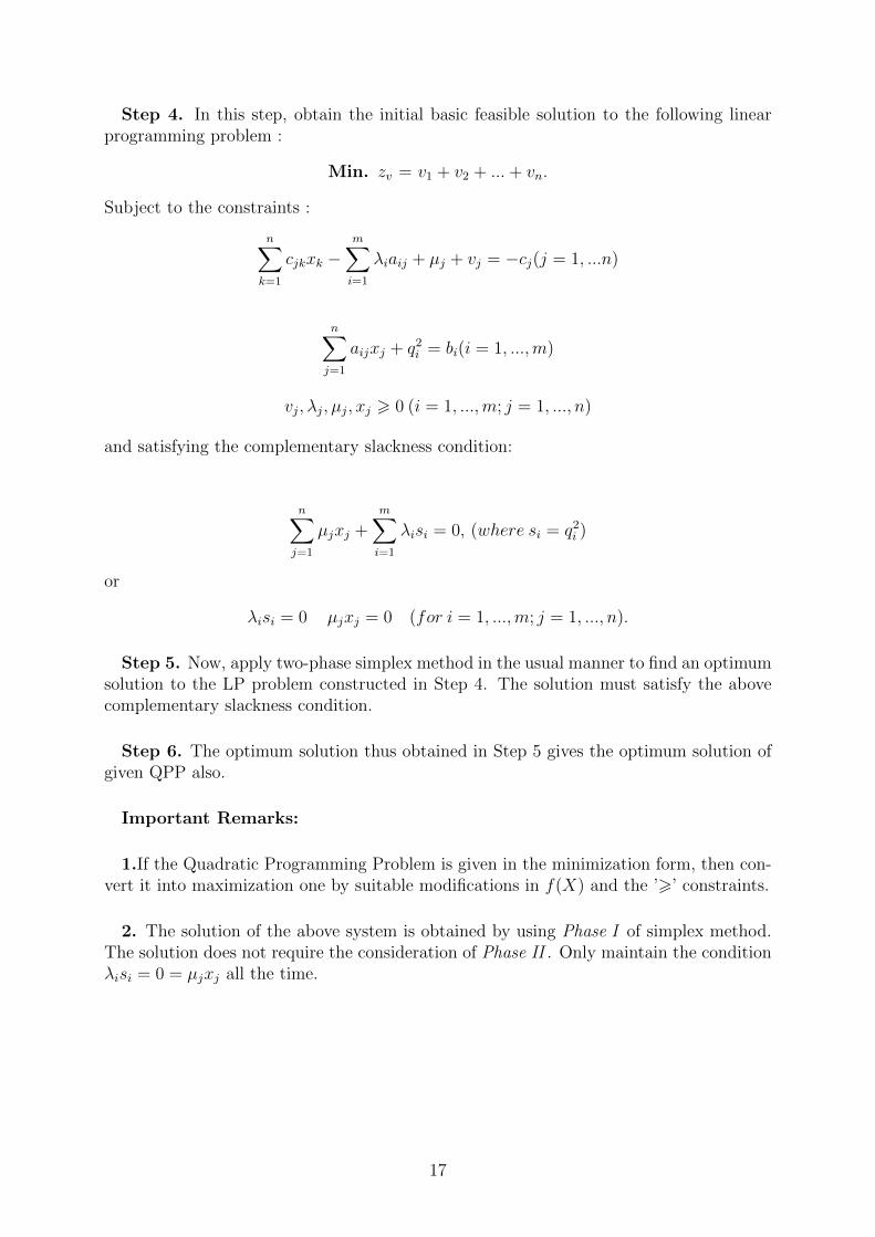
Step 4. In this step, obtain the initial basic feasible solution to the following linearprogramming problem :

Min. zv = v1 + v2 + ...+ vn.

Subject to the constraints :

n∑k=1

cjkxk −m∑i=1

λiaij + µj + vj = −cj(j = 1, ...n)

n∑j=1

aijxj + q2i = bi(i = 1, ...,m)

vj, λj, µj, xj > 0 (i = 1, ...,m; j = 1, ..., n)

and satisfying the complementary slackness condition:

n∑j=1

µjxj +m∑i=1

λisi = 0, (where si = q2i )

or

λisi = 0 µjxj = 0 (for i = 1, ...,m; j = 1, ..., n).

Step 5. Now, apply two-phase simplex method in the usual manner to find an optimumsolution to the LP problem constructed in Step 4. The solution must satisfy the abovecomplementary slackness condition.

Step 6. The optimum solution thus obtained in Step 5 gives the optimum solution ofgiven QPP also.

Important Remarks:

1.If the Quadratic Programming Problem is given in the minimization form, then con-vert it into maximization one by suitable modifications in f(X) and the ’>’ constraints.

2. The solution of the above system is obtained by using Phase I of simplex method.The solution does not require the consideration of Phase II . Only maintain the conditionλisi = 0 = µjxj all the time.

17

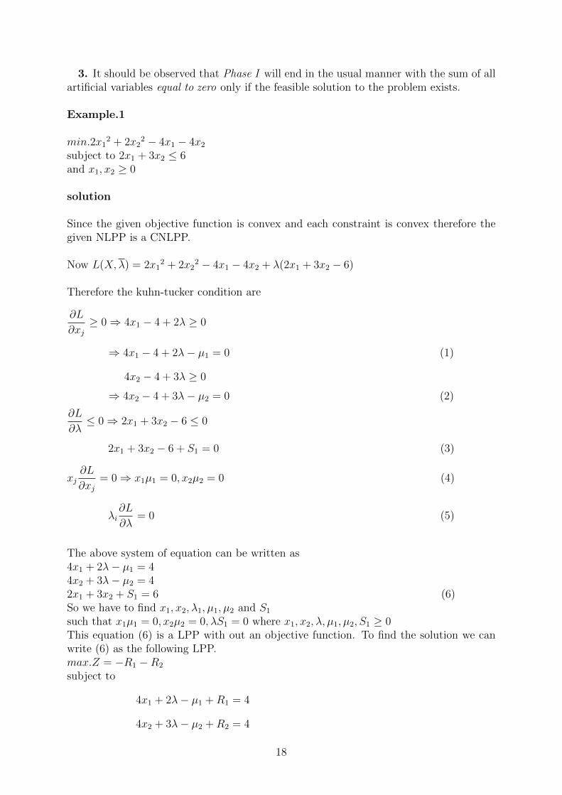
3. It should be observed that Phase I will end in the usual manner with the sum of allartificial variables equal to zero only if the feasible solution to the problem exists.

Example.1

min.2x12 + 2x2

2 − 4x1 − 4x2subject to 2x1 + 3x2 ≤ 6and x1, x2 ≥ 0

solution

Since the given objective function is convex and each constraint is convex therefore thegiven NLPP is a CNLPP.

Now L(X,λ) = 2x12 + 2x2

2 − 4x1 − 4x2 + λ(2x1 + 3x2 − 6)

Therefore the kuhn-tucker condition are

∂L

∂xj≥ 0⇒ 4x1 − 4 + 2λ ≥ 0

⇒ 4x1 − 4 + 2λ− µ1 = 0 (1)

4x2 − 4 + 3λ ≥ 0

⇒ 4x2 − 4 + 3λ− µ2 = 0 (2)

∂L

∂λ≤ 0⇒ 2x1 + 3x2 − 6 ≤ 0

2x1 + 3x2 − 6 + S1 = 0 (3)

xj∂L

∂xj= 0⇒ x1µ1 = 0, x2µ2 = 0 (4)

λi∂L

∂λ= 0 (5)

The above system of equation can be written as4x1 + 2λ− µ1 = 44x2 + 3λ− µ2 = 42x1 + 3x2 + S1 = 6 (6)So we have to find x1, x2, λ1, µ1, µ2 and S1

such that x1µ1 = 0, x2µ2 = 0, λS1 = 0 where x1, x2, λ, µ1, µ2, S1 ≥ 0This equation (6) is a LPP with out an objective function. To find the solution we canwrite (6) as the following LPP.max.Z = −R1 −R2

subject to

4x1 + 2λ− µ1 +R1 = 4

4x2 + 3λ− µ2 +R2 = 4

18

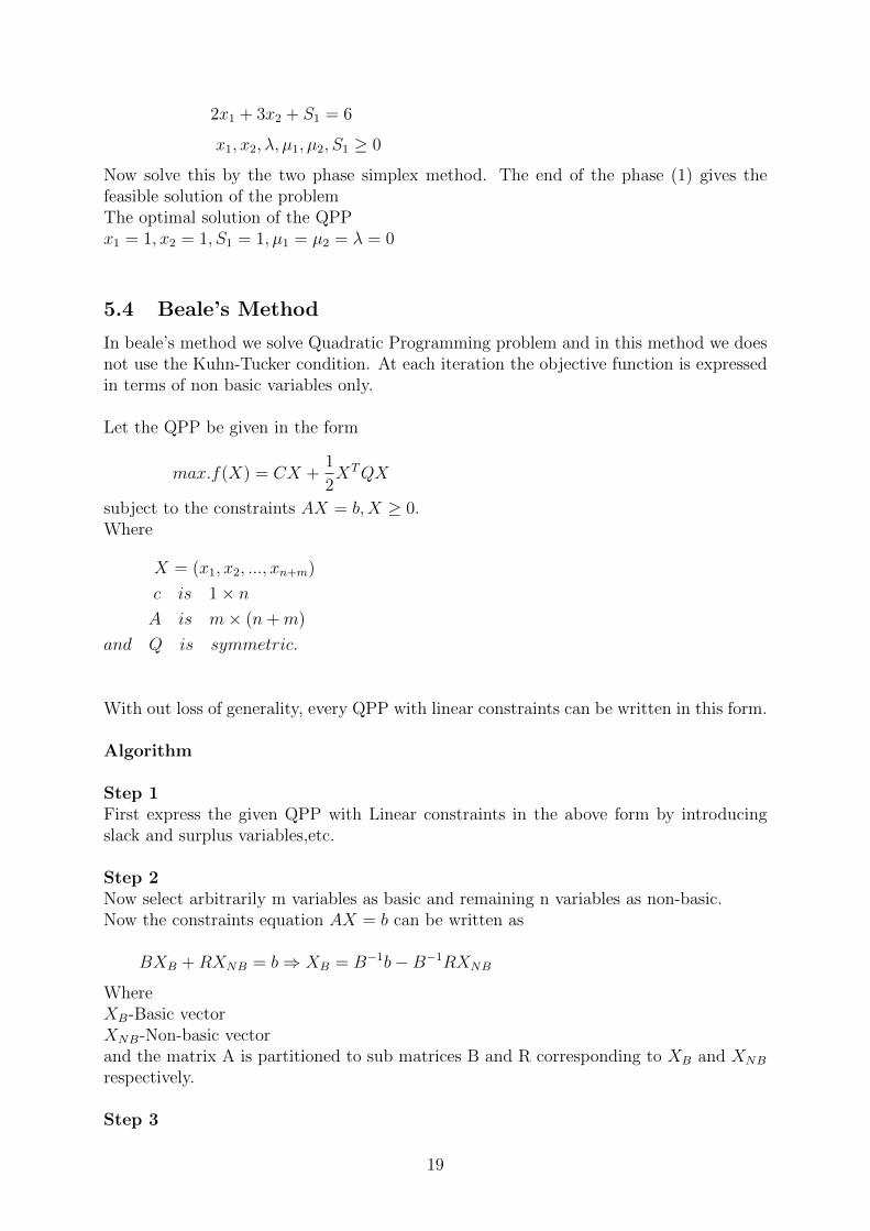
2x1 + 3x2 + S1 = 6

x1, x2, λ, µ1, µ2, S1 ≥ 0

Now solve this by the two phase simplex method. The end of the phase (1) gives thefeasible solution of the problemThe optimal solution of the QPPx1 = 1, x2 = 1, S1 = 1, µ1 = µ2 = λ = 0

5.4 Beale’s Method

In beale’s method we solve Quadratic Programming problem and in this method we doesnot use the Kuhn-Tucker condition. At each iteration the objective function is expressedin terms of non basic variables only.

Let the QPP be given in the form

max.f(X) = CX +1

2XTQX

subject to the constraints AX = b,X ≥ 0.Where

X = (x1, x2, ..., xn+m)

c is 1× nA is m× (n+m)

and Q is symmetric.

With out loss of generality, every QPP with linear constraints can be written in this form.

Algorithm

Step 1First express the given QPP with Linear constraints in the above form by introducingslack and surplus variables,etc.

Step 2Now select arbitrarily m variables as basic and remaining n variables as non-basic.Now the constraints equation AX = b can be written as

BXB +RXNB = b⇒ XB = B−1b−B−1RXNB

WhereXB-Basic vectorXNB-Non-basic vectorand the matrix A is partitioned to sub matrices B and R corresponding to XB and XNB

respectively.

Step 3

19

Express the objective function f(x) in terms of XNB only using the given and additionalconstraint , if any . Thus we observe that by increasing the value of any of the non-basicvariables, the value of the objective function can be improved. Now the constraints onthe new problem become

B−1RXNB ≤ B−1b (since XB ≥ 0)

Thus, any component of XNB can increase only until∂f

∂xNBbecomes zero or one or more

components ofXB are reduced to zero.

Step 5Now we have m+ 1 non-zero variables and m+ 1 constraints which is a basic solution tothe extended set of constraints.

Step 6We go on repeating the above procedure until no further improvement in the objectivefunction may be obtain by increasing one of the non-basic variable.

Example:

Use Beale’s Method to solve following problemmax.Z = 4x1 + 6x2 − 2x1

2 − 2x1x2 − 2x22

suject to x1 + 2x2 ≤ 2

and x1, x2 ≥ 0

Solution:Step:1

Max.Z = 4x1 + 6x2 − 2x12 − 2x1x2 − 2x2

2 (1)

subject to

x1 + 2x2 + x3 = 2 (2)

and x1, x2, x3 ≥ 0taking XB = (x1);XNB =

(x2x3

)and x1 = 2− 2x2 − x3 (3)

Step:2put (3) in (1), we getmax.f(x2, x3) = 4(2− 2x2 − x3) + 6x2 − 2(2− 2x2 − x3)2 − 2(2− 2x2 − x3)x2 − 2x2

2

∂f

∂x2= −2 + 8(2− 2x2 − x3) + 8x2 − 4x2 − 2(2− x3)

∂f

∂x3= −4 + 4(2− 2x2 − x3) + 2x2

Now∂f

∂x2 (0,0)= 10

∂f

∂x3 (0,0)= 4

20

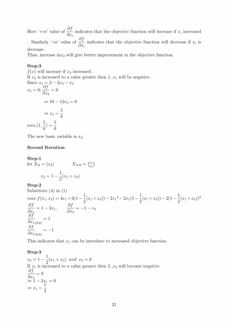
Here ’+ve’ value of∂f

∂xiindicates that the objective function will increase if xi increased

. Similarly ’-ve’ value of∂f

∂xiindicates that the objective function will decrease if xi is

decrease .Thus, increase inx2 will give better improvement in the objective function.

Step:3f(x) will increase if x2 increased .If x2 is increased to a value greater then 1, x1 will be negative.Since x1 = 2− 2x2 − x3x3 = 0;

∂f

∂x2= 0

⇒ 10− 12x2 = 0

⇒ x2 =5

6

min.(1,5

6) =

5

6

The new basic variable is x2.

Second Iteration:

Step:1let XB = (x2) XNB =

(x1x3

)x2 = 1− 1

2(x1 + x3)

Step:2Substitute (4) in (1)

max.f(x1, x3) = 4x1 + 6(1− 1

2(x1 +x3))− 2x1

2− 2x1(1−1

2(x1 +x3))− 2(1− 1

2(x1 +x3))

2

∂f

∂x1= 1− 3x1,

∂f

∂x3= −1− x3

∂f

∂x1 (0,0)= 1

∂f

∂x3 (0,0)= −1

This indicates that x1 can be introduce to increased objective function.

Step:3

x2 = 1− 1

2(x1 + x3) and x3 = 0

If x1 is increased to a value greater then 2 ,x2 will become negative.∂f

∂x1= 0

⇒ 1− 3x1 = 0

⇒ x1 =1

3

21

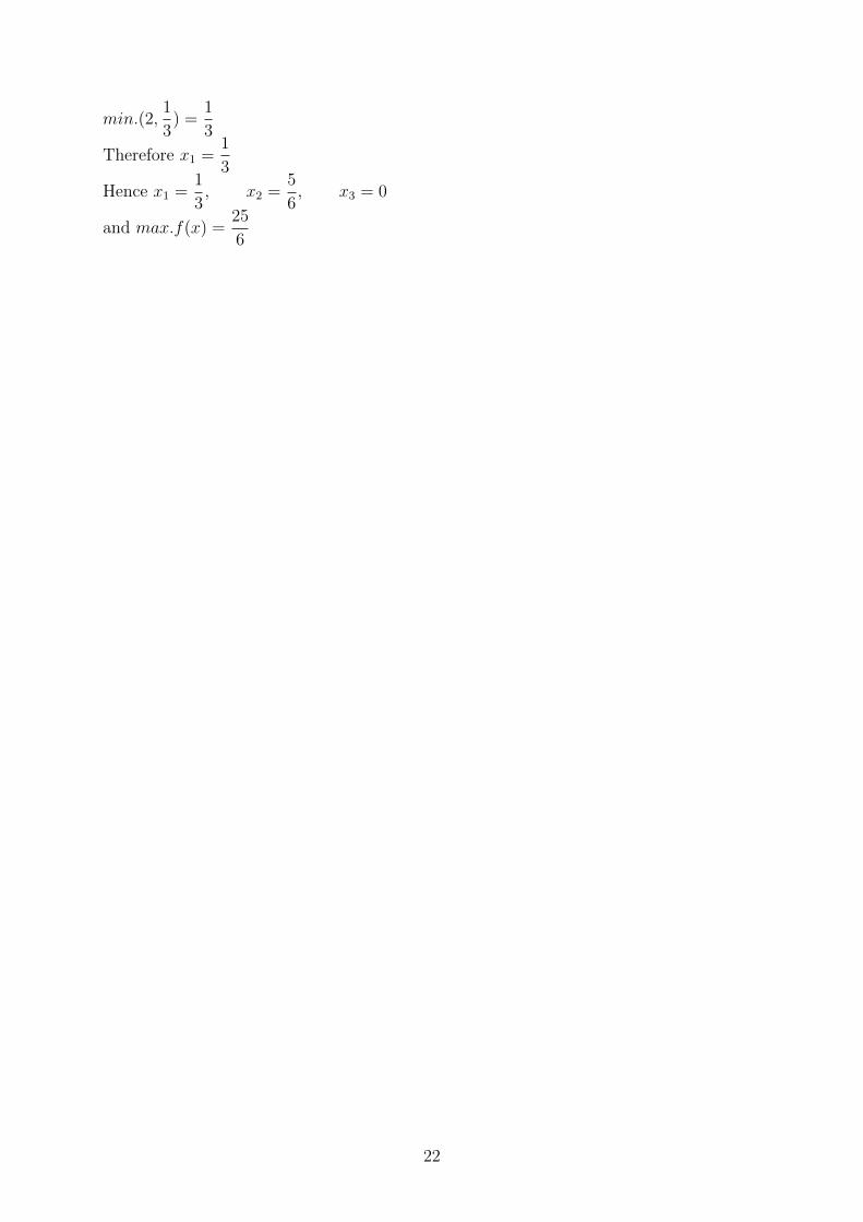
min.(2,1

3) =

1

3

Therefore x1 =1

3

Hence x1 =1

3, x2 =

5

6, x3 = 0

and max.f(x) =25

6

22

CHAPTER 6

6 SEPARABLE PROGRAMMING

6.1 Introduction

Separable Programming deals with such non linear programming problems in which theobjective function as well as all the constraints are separable.We solve an optimizationproblem with non-linear objective function and linear constraints by a linear program.Later we will extend the idea to solve, at least approximately, convex optimization prob-lems with separable non-linear objective functions and convex feasible sets defined byseparable convex functions. The technique, called separable programming, basically re-places all separable convex functions, in objectives and constraints, by piecewise linearconvex functions.

6.2 Separable Function

Definition:A Function f(x1, x2, ..., xn) is said to be separable if it can be expressed asthe sum of n single valued functions f1(x1), f2(x2), ..., fn(xn), i.e.

f(x1, x2, ..., xn) = f1(x1) + f2(x2) + ...+ fn(xn)

.

Example:

g(x1, x2, ..., xn) = c1x1 + ...+ cnxn where c ′s are constants,is a separable function.

g(x1, x2, x3) = x13 + x2

2log(x1 + x3) + x33x2 + e(x1x3)

is not a separable function.

Reducible to Separable Form: Sometimes the functions are not directly separablebut can be made separable by simple substitutions.

Example:max.Z = x1x2

2

Let y = x1x22

Then logy = logx1 + 2logx2Hence the problem becomes

max.Z = Y

subject to

logy = logx1 + 2logx2

which is separable.

23

6.3 Separable Programming Problem

A NLPP in which the objective function can be expressed as a linear combination ofseveral different single variable functions, of which some or all are non-linear, is called aseparable programming problem.

6.4 Reduction of separable programming problem to linear pro-gramming problem

Let us consider the separable programming problem

Max.(Min.)z =n∑j=1

fj(xj)

subject to the constraints :

n∑j=1

gij(xj) 6 bi

xj > 0 (i = 1, 2, ...,m; j = 1, 2, ..., n)

where some or all gij(xj), fj(xj) are non linear.Then the equivalent mixed problem is

Max.(or Min.)z =n∑j=1

n∑k=1

fj(ajk)wjk

subject to the constraints:

n∑j=1

n∑k=1

gij(ajk)wjk 6 bi , i = 1, 2, ...,m

0 6 wj1 6 yj1

0 6 wjk 6 yj.k−1 + yjk where k = 2, 3, ..., kj−1

0 6 wjkj 6 yj.kj−1

kj∑k=1

wjk = 1,

kj−1∑k=1

yjk = 1

yjk = 0 or 1 ; k = 1, 2, ..., kj , j = 1, 2, ..., n

The variables for the approximating problem are given by wjk and yjk .

We can use the regular simplex method for solving the approximate problem under theadditional constraints involving yjk .

24

6.5 Separable Programming Algorithm

Step-1If the objective function is of minimization form, convert it into maximization.

Step-2Test whether the functions fj(xj) and gij(xj) satisfy the concavity (convexity) conditionsrequired for the maximization(minimization) of non-linear programming problem. If thecondition are not satisfied, the method is not applicable, otherwise go to next step.

Step-3Divide the interval 0 6 xj 6 tj (j = 1, 2, ..., n) into a number of mesh points ajk (k =1, 2, ..., Kj) such that aij = 0, aj1 < aj2 < ... < ajKj

= tj

Step-4For each point ajk , compute piecewise linear approximation for each fj(xj) and gij(xj)where j = 1, 2, ..., n; i = 1, 2, ...,m.

Step-5Using the computations of step-4,write down the piece-wise linear approximation of thegiven NLPP.

Step-6Now solve the resulting LPP by two-phase simplex method. For this method considerwi1 (i = 1, 2, ...,m) as artificial variables. Since, the costs associated with them are notgiven, we assume them to be zero.Then,Phase-I of this method is automatically complete.Therefore, the initial simplex table of Phase-I is optimum and hence will be the startingsimplex table for Phase-II.

Step-7Finally, we obtain the optimum solution x∗j of the original problem by using the relations:

x∗j =

Kj∑k=1

ajkwjk (j = 1, 2, ..., n).

25

References

[1] S.D.Sharma, Operations Research, KNRN publication.

[2] Prem Kumar Gupta and Dr.D.S. Hira, Operation Research, S.Chand Publication.

[3] F.S.Hillier and Gerald J. Lieberman , Operations Research.

[4] Martina Vankova, Algorithms for the Solution of the Quadratic Programming Prob-lem, January 2004

26