SAS Software for the Analysis of Epidemiologic · PDF file1 SAS Software for the Analysis of...

1

SAS Software for the Analysisof Epidemiologic Data

Hans-Peter AltenburgGerman Cancer Research Center

Dept. Clinical Epidemiology C0500Im Neuenheimer Feld 280

D-69009 Heidelberg, Germany

2

H.-P. Altenburg: SAS Software for the Analysis of Epidemiologic Data

Outline• Epidemiologic Studies

– case-control studies– cohort studies

• Basic Analysis Methods• Logistic Regression• Conditional Logistic Regression• Log-linear Models• Interactive Model Building

3


Epidemiologic Methods• Generate hypotheses / identify potential targets• Collect data / choose appropriate study design• Prepare data• Design computer models to uncover hidden

structures• Apply models• Conclusion

4


Aims of Epidemiologic StudiesStudy of• Distribution of diseases in human populations• Search for

– disease causing factors /exposure ↔ diseaserelationships

– “risk factors”– earlier exposition / personal characteristics

• Development of– disease prevention hypotheses and strategies

5


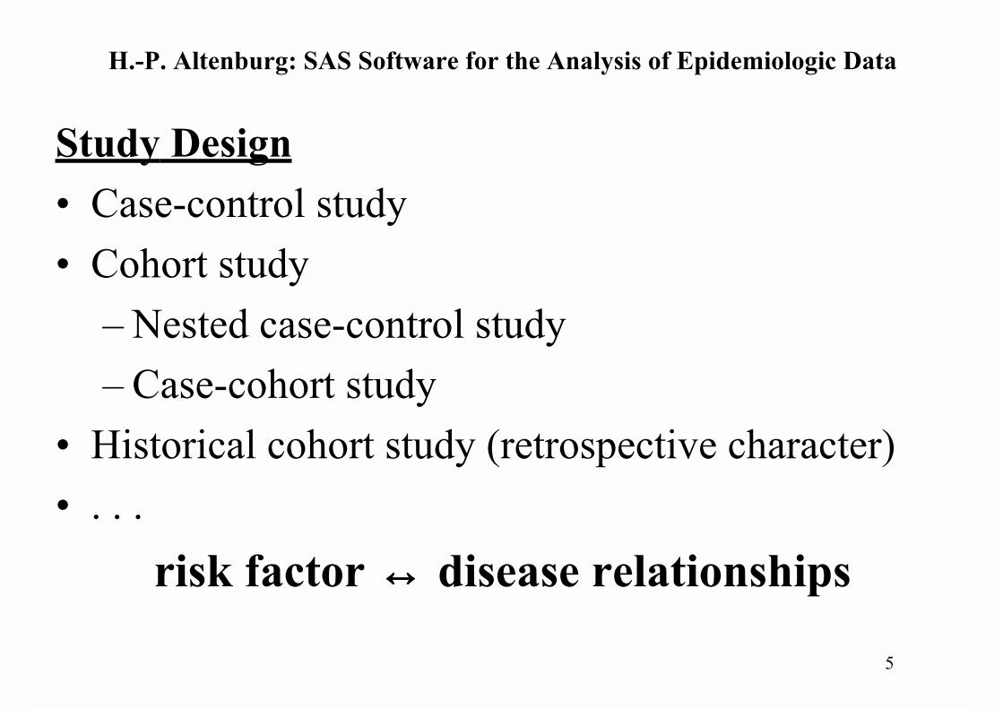
Study Design• Case-control study• Cohort study

– Nested case-control study– Case-cohort study

• Historical cohort study (retrospective character)• . . .

risk factor ↔↔↔↔ disease relationships

6


Examples of Associationsidentified or confirmed using case-control /cohortstudies:• cigarette smoking ↔ lung cancer• blood pressure | blood cholesterol | cigarette

smoking ↔ coronary heart diseases• use of oral contraceptiva ↔↔↔↔ vascular diseases• atomic bomb radiation ↔↔↔↔ risk of leukemia |

various solid tumors• dietary intake ↔↔↔↔ stomach cancer, ...

7


Case-control Studies• retrospective character• collect information about

exposure– from individuals with

disease– but only a fraction of the

population (individuals)without disease

• less efficient than cohortst.

• time compressing– espec. in rare risk groups

Cohort Studies• prospective character• sampling a subset of

individuals over time• occurrence of events of

interest observed overfollow-up’s

Disadvantage:• Duration

8


Goals:

estimate numerical characteristics to measure thesize of influence

Case-control study:odds ratioconfidence limits

Problem:Confounding or effect

modification by measuredcovariatesadjustment for covariates

Cohort study:disease ratesrelative riskconfidence limits

9


Odds ratio (relative odds, OR):is the ratio of odds of disease under expositiondivided by that without exposition.Relative risk (RR):is the ratio of the risk of disease in an exposedcohort to the risk of disease in an unexposedcohort (over the same defined time interval).Rare diseases: OR approximates RR.Interpretation:• risk measure >1: exposition increases risk• risk measure <1: exposition decreases risk

10

H.-P. Altenburg: SAS Software for the Analysis of Epidemiologic DataBasic Analysis Methods

Basic Analysis Methods:Epidemiologic data appear as counts⇒ summarised in contingency tablessimple measures:

• odds ratios• relative risks• disease rate differences• summarised risk measures (Mantel-Haenszel)

11

H.-P. Altenburg: SAS Software for the Analysis of Epidemiologic DataBasic Analysis Methods - Realisation within the SAS System

Realisation using SAS procedure: FREQOptions: RELRISK, CMH, RISKDIFFSAS statements:

PROC FREQ DATA=dset ;TABLES (strata)*(exposure)*(yesill) ;TABLES (exposure)*(yesill) ; / NOPERCENT RELRISK CMH CHISQ RISKDIFF ; /* Risk difference - cohort study */EXACT RROR ;WEIGHT &weight ; RUN ;

12

H.-P. Altenburg: SAS Software for the Analysis of Epidemiologic DataBasic Analysis Methods - Realisation within the SAS System

Realisation using SAS macro language:

%MACRO epibase(dset, yesill, exposure, byvar, weight, exact, study) ;/* -------------------------------------------------- Basic epidemiologic measures for case-control studies (OR) cohort studies (RR) -------------------------------------------------- */ PROC FREQ DATA=&dset ;%IF %LENGTH(&byvar)>0 %THEN TABLES (&byvar)*(&exposure)*(&yesill) ; %ELSE TABLES (&exposure)*(&yesill) ; / NOPERCENT RELRISK CMH CHISQ%IF %UPCASE(&study)=COHORT %THEN %DO ; /* Cohort study only */ RISKDIFF /* Risk difference */ %END ; ;%IF %UPCASE(&exact)=YES OR %UPCASE(&exact)=Y %THEN EXACT RROR ; ;%IF %LENGTH(&weight)>0 %THEN WEIGHT &weight ; ;RUN ;%MEND ;

13

H.-P. Altenburg: SAS Software for the Analysis of Epidemiologic Data Basic Analysis Methods - Realisation within the SAS System

Further Tools:• Subgrouping• subgroup selection• contingency table input

e.g. D+ D-Exp. + 5 95Exp. - 1 99

14

H.-P. Altenburg: SAS Software for the Analysis of Epidemiologic DataLogistic Regression

Logistic Regression:

Goal:Find best fitting and biologically reasonablemodel to describe the relationship betweenoutcome (disease) and a set of independentexplanatory variables.

P(Disease +|X=x)=exp(β0 + β1 x)/(1+ exp(β0 + β1 x))

15

H.-P. Altenburg: SAS Software for the Analysis of Epidemiologic Data Logistic Regression

orlogit(P(Disease +|X=x)) = β0 + β1 x

Interpretation of the regression coefficient:β1 = log odds

exp(β1 ) = odds ratio

16


Realisation using SAS procedure: LOGISTICStd. Options: CL, PLCL, RISKLIMITS,

RSQUARE, DESCENDING

%MACRO epiLR(dset, yesill, exposure, covars, byvar, freq, descending);/* ----------------------------------------- Logistic Regression using procedure LOGISTIC ----------------------------------------- */PROC LOGISTIC DATA=&dset%IF &UPCASE(&descending)=DESCENDING OR &UPCASE(&descending)=D %THEN DESCENDING ; %ELSE ;;MODEL &yesill = &exposure &covars / CL PLCL RISKLIMITS RSQUARE ;%IF %LENGTH(&freq)>0 %THEN WEIGHT &freq ; ;RUN ;%MEND ;

17


Output and additional applications:• Odds ratios• Confidence limits (Wald, profile likelihood)• classification

– predicted probabilities (Options OUT=..., P=...)– (ROC curve, etc. |Options OUTROC, GPLOT

procedure, ...)• interactive model building features

18


Further Aspects:• Interaction terms must be included with a new

variable when using PROC LOGISTIC:e.g. interaction age ↔ exposition:create a new variable in a preceding data step:

i_ageexp=age*exposition ;(not up V 8)

• Alternative approach:use SAS procedure GENMOD

19

H.-P. Altenburg: SAS Software for the Analysis of Epidemiologic Data Logistic Regression - Procedure GENMOD

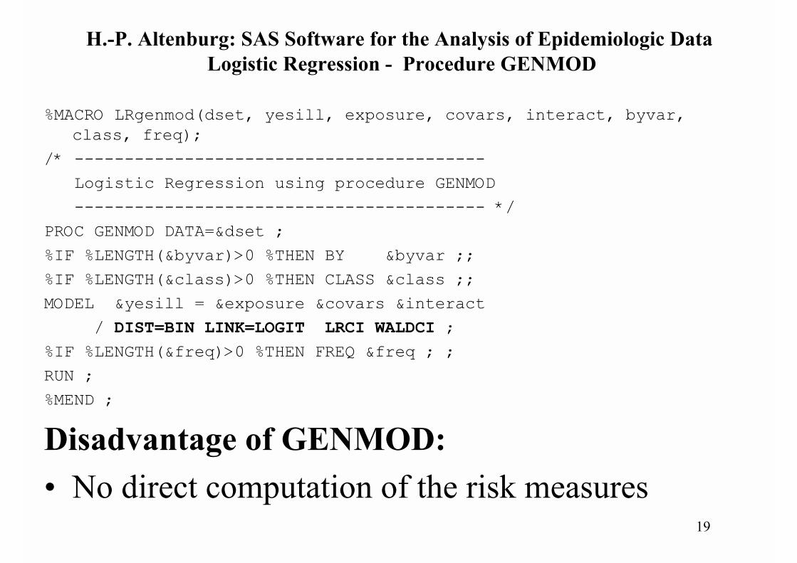
%MACRO LRgenmod(dset, yesill, exposure, covars, interact, byvar,class, freq);

/* ----------------------------------------- Logistic Regression using procedure GENMOD ----------------------------------------- */PROC GENMOD DATA=&dset ;%IF %LENGTH(&byvar)>0 %THEN BY &byvar ;;%IF %LENGTH(&class)>0 %THEN CLASS &class ;;MODEL &yesill = &exposure &covars &interact / DIST=BIN LINK=LOGIT LRCI WALDCI ;%IF %LENGTH(&freq)>0 %THEN FREQ &freq ; ;RUN ;%MEND ;

Disadvantage of GENMOD:• No direct computation of the risk measures

20

H.-P. Altenburg: SAS Software for the Analysis of Epidemiologic Data Conditional Logistic Regression

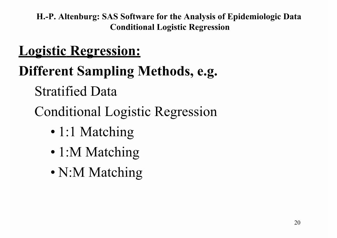
Logistic Regression:Different Sampling Methods, e.g.

Stratified DataConditional Logistic Regression

• 1:1 Matching• 1:M Matching• N:M Matching

21

H.-P. Altenburg: SAS Software for the Analysis of Epidemiologic Data Conditional Logistic Regression - 1:1 Matching

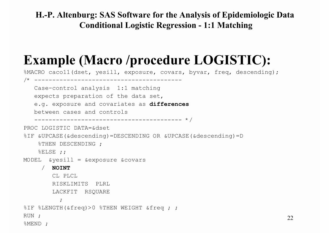
Case-control studies:1:1 matchingLikelihood:

L1 =exp( β1 (x1 - x0))/(1+ exp( β1 (x1 - x0)))⇒⇒⇒⇒preparation of the data set:

– compute differences of the covariatesuse procedure LOGISTIC with option NOINT!

22

H.-P. Altenburg: SAS Software for the Analysis of Epidemiologic Data Conditional Logistic Regression - 1:1 Matching

Example (Macro /procedure LOGISTIC):%MACRO caco11(dset, yesill, exposure, covars, byvar, freq, descending);/* ----------------------------------------- Case-control analysis 1:1 matching expects preparation of the data set, e.g. exposure and covariates as differences between cases and controls ----------------------------------------- */PROC LOGISTIC DATA=&dset%IF &UPCASE(&descending)=DESCENDING OR &UPCASE(&descending)=D %THEN DESCENDING ; %ELSE ;;MODEL &yesill = &exposure &covars / NOINT CL PLCL RISKLIMITS PLRL LACKFIT RSQUARE ;%IF %LENGTH(&freq)>0 %THEN WEIGHT &freq ; ;RUN ;%MEND ;

23

H.-P. Altenburg: SAS Software for the Analysis of Epidemiologic Data Conditional Logistic Regression - 1:M-, N:M- Matching

Matched case-control: 1:M- / N:M-MatchingUse SAS procedure PHREGPrepare data set:MODEL time*status = list of risk factors / TIES=... ;time: dummy variable: time(case)<time(control) per stratum

e.g. time(case)=1, time(control)=2status: controls have status censored, e.g. status(control)=0TIES-Statement:

1:M-Matching: TIES=BRESLOWN:M-Matching: TIES=DISCRETE

24

H.-P. Altenburg: SAS Software for the Analysis of Epidemiologic Data Conditional Logistic Regression - 1:M-, N:M- Matching

SAS Macro:%MACRO cacoNM(dset, time, yesill, vnotill,exposure, covars, strata, study);/* -----------------------------------------

Case-control analysis 1:M / N:M matching expects preparation of the data set study: CACO1M | CACONM

----------------------------------------- */PROC PHREG DATA=&dsetMODEL (&time)*(&yesill)(&vnotill) = &exposure &covars / RISKLIMITS%IF %UPCASE(&study)=CACO1M %THEN TIES=BRESLOW ;; %ELSE TIES=DISCRETE ;;STRATA &strata ;RUN ;%MEND ;

strata variable: e.g. use age

25

H.-P. Altenburg: SAS Software for the Analysis of Epidemiologic DataLog-linear Models

Log-linear ModelsFocus:

Search for statistical dependencies / independence(categorical data)

SAS proceduresCATMOD (linear models) andGENMOD (generalised linear models)

26

H.-P. Altenburg: SAS Software for the Analysis of Epidemiologic DataLog-linear Models

Macro log-linear model (PROC CATMOD):%MACRO Mloglin(dset, v1, v2, v3, v4, v5,llinmod, weight);* ----------------------------------------- Log-linear modelling ----------------------------------------- */PROC CATMOD DATA=&dset ;%IF %LENGTH(&weight>0) %THEN WEIGHT &weight ;;MODEL (&v1)*(&v2) %IF %LENGTH(&v3>0) %THEN *(&v3) ; %IF %LENGTH(&v4>0) %THEN *(&v4) ; %IF %LENGTH(&v5>0) %THEN *(&v5) ; =_RESPONSE_ / NOPROFILE NORESPONSE NOITER NOPARM ;%IF %LENGTH(&llinmod>0) %THEN LOGLIN &llinmod ;;RUN ;%MEND ;

%mloglin(smoker,cigrets,cigars,inhale,,,cigrets|cigars|inhale,counts)

27

H.-P. Altenburg: SAS Software for the Analysis of Epidemiologic Data Log-linear Models - Poisson Model

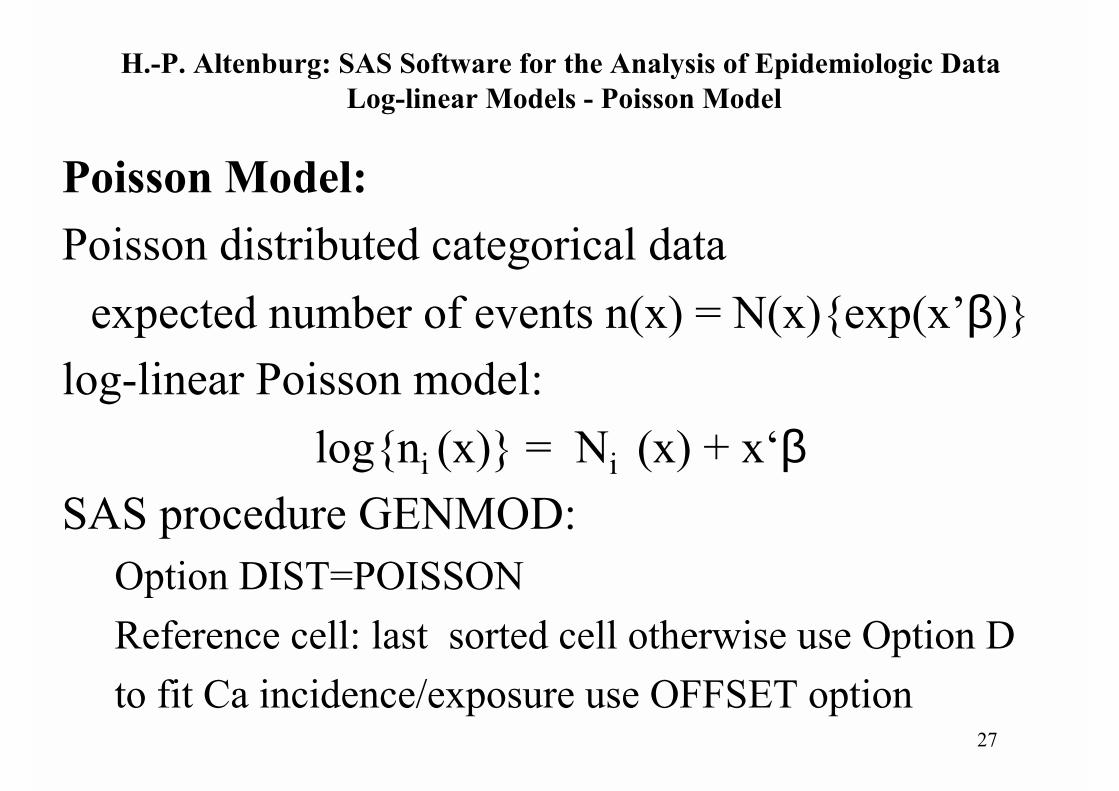
Poisson Model:Poisson distributed categorical data

expected number of events n(x) = N(x){exp(x’β)}log-linear Poisson model:

log{ni (x)} = Ni (x) + x‘βSAS procedure GENMOD:

Option DIST=POISSONReference cell: last sorted cell otherwise use Option Dto fit Ca incidence/exposure use OFFSET option

28

H.-P. Altenburg: SAS Software for the Analysis of Epidemiologic Data Log-linear Models - Poisson Model

%MACRO LlinPoi(dset, objective, exposure, covars, class, order,offset, freq);

* ----------------------------------------- Log-linear modelling Poisson model using PROC GENMOD ----------------------------------------- */PROC GENMOD DATA=&dset%IF %LENGTH(%UPCASE(&order))=DATA OR %LENGTH(%UPCASE(&order))=D %THEN ORDER=DATA ;;%IF %LENGTH(&class>0) %THEN CLASS &class ;;MODEL &objective = &exposure &covars / DIST=POISSON LINK=LOG%IF %LENGTH(&offset>0) %THEN OFFSET=&offset ;;%IF %LENGTH(&freq>0) %THEN FREQ &freq ;;RUN ;%MEND ;

29

H.-P. Altenburg: SAS Software for the Analysis of Epidemiologic DataModel Buiding

Model Building Processrelated with a data mining process:find exposure ↔ disease relationships⇒

search for the most parsimonious modelthat still explains exposure-disease associations

More variables included→ greater std errors→ more dependent on the observed data

30

H.-P. Altenburg: SAS Software for the Analysis of Epidemiologic Data Model Buiding

Variable Selection Process:• Start with a detailed univariate analysis

– outcome ↔ all relevant variables– contingency tables, OR’s / RR’s, ...– p-value limit: 0.25– graphical analysis

• Look for interactions• Confounding assessment / adjustment• ...Danger: overfitting, numerically instable, ...

31

H.-P. Altenburg: SAS Software for the Analysis of Epidemiologic Data Model Buiding

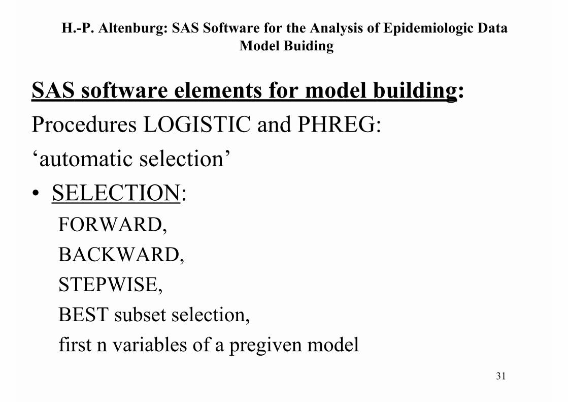
SAS software elements for model building:Procedures LOGISTIC and PHREG:‘automatic selection’• SELECTION:

FORWARD,BACKWARD,STEPWISE,BEST subset selection,first n variables of a pregiven model

32


Summary

• Many SAS procedures support the analysis ofepidemiologic data

• Model building is an interactive process• Minor experienced SAS user need guided software

support• SAS/AF environment can help to guide

unexperienced users

33


To the macrossee webpage,for the exact URL, etc.send an E-mail to:

[email protected]

34


Any comments or questions?

Thank you for your attention!

;-)

On a SAS AF Application for the Analysis of Epidemiologic Data

Hans-Peter AltenburgGerman Cancer Research Center

Dep. Clinical Epidemiology C0500Im Neuenheimer Feld 280

D-69009 Heidelberg, Germany

AbstractThe paper shows the realisation of an application for epidemiologic research problems on thebasis of SAS/AF. The application allows the determination of simple risk measures likerelative risks or odds ratios for cohort and case-control studies as well as the application ofthe Mantel Haenszel procedure. Moreover the use of more complex techniques such aslogistic regression using the SAS procedure LOGISTIC, GENMOD or PHREG in theconditioned case can be applied. Loglinear models analysis can be performed on the base ofthe SAS procedure CATMOD. All techniques are embedded in an SAS/AF environment.

1. IntroductionEpidemiologic methods study the distribution of diseases in human populations and look forfactors that can be the cause for the observed disease distributions. This scientific process hasmany of aspects we know from data mining strategies. Mainly two general types ofepidemiologic studies are established, cross-sectional or longitudinal studies, or with a moreepidemiologic framework,! case-control studies, and! cohort studies.

Most data mining methods have been developed for the analysis of cross sectional data. Butmany epidemiologic research is focused on longitudinal data structures. In the following wedescribe some methods and procedures of a SAS/AF application that can be used for theanalysis of mainly cross-sectional data structures. The extension of the system for the analysisof longitudinal data structures is planned for the future. The aim of epidemiologic studies is to search for associations between the outcome ofdiseases or more generally the occurrence of health related events in relation to some earlierexposure factors or personal characteristics and to identify disease prevention hypotheses andstrategies. Case-control studies have a more retrospective characteristic, starting from theappearance of a disease one looks at possible causes in the past, in contrast to cohort studies,that mostly involve as a key element the follow up of individuals over time to study anoutcome in relation to some earlier exposure factor or a fixed host characteristic such asgenotype. In case of precedence the cohort study identification to the follow up, the studytermination is called prospective, whereas one is talking of a retrospective cohort study whenthe cohort study identification starts after a conceptual follow up period. Case-control designs are used for studying risk factor or exposure disease relationships bycollecting information about exposure from subjects with disease but only from a fraction ofindividuals who did not develop the disease. Such a design has advantages against the cohortdesign described in the following paragraph, but is less efficient. One advantage lies in thecompression of time needed to complete the study, especially for such risk groups where onewould expect to find only few cases. The goal of case-control studies is to identify risk factorsthat are related to the disease under consideration and to estimate numerical characteristicslike odds ratios to measure the size of the influence of the exposure factor on the devilment ofthe disease. According to the nonrandomized character of the study design, the analysis ofsuch studies must turn attention to the possibility of confounding or effect modification bymeasured covariates.

Cohort studies involve the sampling of a subset of individuals over time of a large populationof individuals. The occurrence of events of interest is observed over distinct follow upperiods. The purpose of these studies is the estimation of disease rates and the relationshipsbetween such rates and individual characteristics or exposures. Special study designs includecase cohort or nested case-control studies. Epidemiologic studies require a clear protocol describing important aspects such as studyobjectives, design choices, performance goals, monitoring and analysis procedures. Datacollection and management have to be carefully performed with as much automation aspossible and practicable. The use of corresponding software systems, such as SAS software,can enhance a distinct state of study quality. SAS software can be established in all phases ofepidemiologic studies, e.g. the design, data base management as well as the analysis. But inthis paper we concentrate our attention on the realisation of interactive analysis procedures forepidemiologic data sets and give a short overview on SAS procedures which can be usedthereof. All methods discussed below are realized in SAS macro procedures that areembedded in a SAS/AF environment. 2. Basic Analysis Methods In many situations epidemiologic data appear as counts resulting from tabulating discretevariables or categorized quantitative variables. In such situations the data are summarized incontingency tables, 2x2-tables or stratified 2x2-tables. The basic analysis methods for case-control or cohort studies are the use of contingency tables and the computation of simplemeasures such as

! odds ratios (case-control study),! relative risks (cohort study),! disease rate differences (cohort study) or! summarized risk measures according to the Mantel-Haenszel procedure.

The realisation of this type of analysis can be performed with the SAS procedure FREQ usingoptions like

! RISKDIFF, to get disease rate differences! RELRISK or CMH, to get odds ratios or relative risks including the use of the Mantel-

Haenszel procedure in case of a stratified analysis.An interactive SAS/AF environment is helpful to support SAS inexperienced users to get acorrect analysis with the right option statement. Furthermore the application allows thecalculation of exact confidence limits as well as exact p-values using the EXACT statement ofthe procedure FREQ. In case of existing contingency tables with only absolute figuresavailable, the application allows the input of the contingency table in a dialog form betweenuser and system. Furthermore a tool for subgrouping and special subgroup selection isincluded to support the search and identification of confounders.

3. Logistic RegressionThe objective of a logistic regression approach is to find the best fitting and most biologicallyreasonable model to describe the relationship between the disease outcome and a set ofindependent, predictor or explanatory variables. The outcome variable is categorical, mostlybinary or dichotomous, e.g. disease observed („D+“) vs. disease not observed („D-„). In caseof one single explanatory variable X, the logistic regression model can be expressed in theconditioned form

p(x) = P(D+ | X=x ) = exp("0 + "1 x)/(1+ exp("0 + "1 x)),meaning that we express the conditioned probability (given the explanatory variable X=x) thatthe disease is apparent by a logistic function. Performing a logit transformation for both sidesof the equation leads to

logit(p(x)) = "0 + "1 x.

Instead of the logistic function many other probability distributions could be proposed for theanalysis of binary outcomes. But there are at least two primary reasons for choosing thelogistic function: (i) it is from a mathematical point of view an easy to realize function, and,(ii) it has itself a biologically meaningful interpretation. The importance of the logittransformed relationship is, that it has many of the desirable properties of a linear regressionmodel (e.g. linear in the parameters, continuous with range -# to +# depending on the rangeof X. An important difference between linear and logistic regression concerns the conditioneddistribution of the outcome variable. In a linear regression the error of the outcome variable isnormally distributed with expectation zero and constant variance. With a dichotomousoutcome variable the error distribution has mean zero and variance equal to the variance of abinomial distribution p(x)(1-p(x)). The conditioned distribution of the outcome variablefollows therefore binomial distribution with probability given by the conditioned mean p(x).The model can easily extended to several explanatory variables.The regression coefficient "1 in the logistic regression model can be interpreted as log odds,or, the expression exp("1 ) as odds ratio when considering a dichotomous independentvariable. Similarly one can interpret the regression coefficients in case of polytomous data. Inthis case one has additionally to specify so called dummy (design) variables.The logistic regression technique is widely used in epidemiology for identifying risk factorsassociated with disease outcomes and with the identification of potentially importantcovariates in exploratory data analysis or a data mining process.Logistic regression can be performed in the SAS system using the procedure LOGISTIC. TheSAS/AF application allows many different applications of the procedure, such as thecomputation of

! a simple binary logistic regression,! logistic regression with an ordinal response variable,! odds ratios with confidence limits,! predicted probabilities,! data classification including the plot of ROC curves,! 1:1 matched data of a case-control study, and! interactively model building feature.

Furthermore the application allows the inclusion of higher order interaction terms. Theinteraction terms can be created in a separate data step. Alternatively the use of the procedureGENMOD is offered to the user, to fit a logistic regression with interaction terms orqualitative variables and furthermore longitudinal data. The objective variable will then bechanged into the binomial form required by the procedure GENMOD. The model buildingaspects of the application are described in a separate section below.

4. Conditioned Logistic RegressionThe conditioned logistic regression is an important extension of the standard logisticregression model. It is used in the analysis of stratified samples, where, for example,covariables are controlled for by defining post hoc stratification variables. The mostfrequently encountered study design is the matched case-control study, such as 1:N matchingor N:M matching.The underlying basic idea is the expansion of the standard logistic model by inclusion ofstratification variables. The model is extended by one design variable for the stratum specificeffect and constant slope across strata for covariates. The new model does not representanything particularly new or difficult for the investigator familiar with the standard logisticregression model. Problems can arise when the number of strata increases and the number ofcases per strata remains fixed.The SAS procedure PHREG can be used to fit a conditional logistic regression model toinvestigate the relationship between an disease outcome and a set of influence factors. Using a

SAS macro the data set is prepared for the application of the procedure PHREG, which wasoriginally designed for the analysis if survival times. So, for example we have to create twodummy variables: a variable t_status representing the time, with t_status=1 for all cases andthe value t_status=2 for all controls, and a variable representing the censoring status whereasthe controls are treated as censored. The TIES option in the MODEL statement of the PHREGprocedure is used to indicate the type of matching: TIES=DISCRETE for N:M matching orTIES=BRESLOW for 1:M matching and the TIES default for 1:1 matching case. TheSAS/AF application gives an easy handling tool for the analysis of conditional logisticregression problems.

5. Log-linear ModelsA more sophisticated approach for the analysis of contingency tables is the application of log-linear models. The objective of these procedures is rather hypothesis testing analogously toANOVA and regression techniques and not to the fit of certain models and the estimation ofthe corresponding parameters. The focus of a log-linear analysis lies in the search forstatistical dependence or independence. Log-linear modeling of categorical data is an analogto the correlation analysis of quantitative variables.There are three underlying sampling models for the observed counts possible:

! the Poisson model, meaning the observed counts stem from independent Poissonrandom variables,

! the multinomial model, and! the product multinomial model.

Log linear models can be analyzed in the SAS system by using the CATMOD procedure. TheSAS/AF application allows contingency tables up to five dimensions with user specifiedinteraction terms or nested effects.Generalized linear models can also be performed using the GENMOD procedure.

6. Model BuildingOften, epidemiologic studies such as multicenter cohort studies contain large data sets withmany independent variables that could be included in a model. Thus an additional objective ofthese studies involves the search for the most parsimonious model that still explains theassociation between exposure and disease outcome. One reason for minimizing the number ofvariables in a model is the numerical instability we get when including many variables in amodel. The more variables we have include in a model, the greater the estimated standarderrors become and the more dependent the model becomes on the observed data. But manyepidemiologists try first to include all scientifically relevant variables into the model. Theobjective for this approach is to provide as complete control of confounding as possiblewithin the data base. The reason can be found in the fact that it is possible for individualvariables not to exhibit strong confounding, but when taken collectively, considerableconfounding can be found in the data. Only one problem appears with this approach. Themodel is overfitted and numerically instable, which follows from large estimated coefficientsand standard errors.A variable selection process should therefore start with a detailed univariate analysis of eachvariable against the outcome variable, e.g. for nominal, ordinal or continuous variables withonly few integer values performing a contingency table with the calculation of the chi-squaretest and the estimation of odds ratios or relative risks using one level as reference group. Fortrue quantitative variables a univariate logistic regression variable selection procedure or a t-test based selection procedure may be useful to find out which variables should included in apreliminary set of model variables. A graphical analysis might also be useful. Bendel andAfifi (1977) propose a limit for the p-value of 0.25. A larger limit leads to the inclusion of not

so important variables. The more traditional level of 0.05 for the p-value often fails to includeimportant variables.The SAS/AF application allows such a one-dimensional description of the relevant dataadditionally to the basic methods described in section 2.The SAS procedures LOGISTIC and PHREG allow variable selection methods, such as

! forward selection,! backward selection,! stepwise selection,! best subset selection, or! the subset of the first n variables of a pregiven model.

Model building is an interactive process. A minor experienced SAS user needs thereforeguided support in performing a data analysis. Using the SAS/AF environment we realizedthese aspects and the user can interactively decide which variables and which procedure hewants to use or to be included in the model.

Literature

1. Bendel, R.B. and Afifi, A.A. (1977): Comparison of stopping rules in forward regression.Journal of the American Statistical Association 72, 46-53

2. Hosmer, D.W. and Lemeshow, S. (1989): Applied logistic regression. Wiley, New York3. SAS/AF Software: FRAME Application Development Concepts. Version 6, 1st edition,

SAS Institute Inc., Cary N.C.4. SAS Guide to Macro Processing. Version 6, 2nd edition, SAS Institute Inc., Cary N.C.5. SAS/STAT User’s Guide, Vol. 1 and Vol. 2. Version 6, 4th Edition. SAS Institute Inc., Cary

N.C.

SAS Software for the Analysis of Epidemiologic · PDF file1 SAS Software for the Analysis of...

Documents

Transcript of SAS Software for the Analysis of Epidemiologic · PDF file1 SAS Software for the Analysis of...