SAR image formation toolbox for MATLAB -...

SAR image formation toolbox for MATLAB

LeRoy A. Gorham and Linda J. Moore

Air Force Research Laboratory, Sensors Directorate2241 Avionics Circle, Bldg 620, WPAFB, OH 45433-7321

ABSTRACT

While many synthetic aperture radar (SAR) image formation techniques exist, two of the most intuitive methodsfor implementation by SAR novices are the matched filter and backprojection algorithms. The matched filter and(non-optimized) backprojection algorithms are undeniably computationally complex. However, the backprojec-tion algorithm may be successfully employed for many SAR research endeavors not involving considerably largedata sets and not requiring time-critical image formation. Execution of both image reconstruction algorithmsin MATLAB is explicitly addressed. In particular, a manipulation of the backprojection imaging equations issupplied to show how common MATLAB functions, ifft and interp1, may be used for straight-forward SARimage formation. In addition, limits for scene size and pixel spacing are derived to aid in the selection of anappropriate imaging grid to avoid aliasing. Example SAR images generated though use of the backprojectionalgorithm are provided given four publicly available SAR datasets. Finally, MATLAB code for SAR imagereconstruction using the matched filter and backprojection algorithms is provided.

Keywords: SAR, image formation, matched filter, backprojection algorithm

1. INTRODUCTION

Over the past four decades, numerous image formation algorithms have been developed with varying levels ofcomplexity and accuracy. However, these algorithms have a steep learning curve for SAR novices. In thispaper, we introduce two algorithms - matched filter and backprojection - implemented in MATLAB, whichare very simple to understand. A benefit of matched filter image reconstruction is that the method offersoptimization of the signal-to-noise ratio (SNR).1 Use of the matched filter requires a hypothesis regarding atarget’s characteristics; these assumptions yield a specifically designed filter that will ideally match to the target.While the matched filter algorithm is intuitive and straight-forward, the generation of a 2D SAR image usingthis technique requires O(N4) operations. For most practical situations, the computational complexity of thematched filter algorithm renders use of the method unrealistic. However, understanding of this fundamentalimaging algorithm is extremely beneficial, especially for the SAR novice.

While several techniques exist for SAR image generation, two commonly employed approaches worth notinghere are the polar format and backprojection algorithms. These algorithms differ in regards to the tradeoffbetween computational complexity and image quality.2,3 The polar format algorithm4,5 for SAR image recon-struction is similar to computer-aided tomography imaging techniques.6,7,8 Polar format reconstruction employsa direct 2D Fourier transform, which provides the opportunity to take advantage of the extremely efficient fastFourier transform. Polar format image reconstruction requires O(N2 logN) operations given an NxN SAR im-age. While more computationally effective than the backprojection algorithm, the polar format imaging methodinvolves an approximation of the received signal phase. This approximation introduces errors into the final re-constructed SAR image. Several correction techniques have been suggested as a means of improving the accuracyof SAR images generated via polar format reconstruction.9,10

Another frequently used image formation technique is the backprojection algorithm.7,11 A distinct advantageof the backprojection algorithm is the ability to form SAR images as phase history is collected, pulse by pulse,and to integrate newly obtained information into the SAR image as it becomes available. The backprojectionalgorithm is computationally expensive, however, as it requires O(N3) operations for an NxN SAR image. For-tunately, the backprojection algorithm lends itself naturally to parallel processing. Backprojection has recently

Further author information: (E-mail: [email protected] and [email protected])

Algorithms for Synthetic Aperture Radar Imagery XVII, edited by Edmund G. Zelnio, Frederick D. Garber, Proc. of SPIE Vol. 7699, 769906 · © 2010 SPIE · CCC code: 0277-786X/10/$18 · doi: 10.1117/12.855375

Proc. of SPIE Vol. 7699 769906-1

Downloaded from SPIE Digital Library on 23 Jun 2011 to 222.197.180.163. Terms of Use: http://spiedl.org/terms

been implemented on graphics processing units (GPUs),12,13 which provide inexpensive platforms for parallelcomputing.

Several methods have been proposed as a means of reducing the computational complexity of the backpro-jection algorithm while retaining the advantages of this image formation approach.14,15,16,17 Many of these fastbackprojection algorithms are flexible, providing manners in which image quality may be acceptably sacrificed inorder to further improve data processing time. These image formation algorithms, several of which are favorablegiven wide bandwidths and large synthetic apertures, offer decreased computational complexities of O(N5/2)14

and O(N2 logN).15,16,17 Non-optimized backprojection imaging may be impractical for exceptionally large datasets with time-critical image formation requirements; however, knowledge of this simple SAR imaging techniqueis undoubtedly valuable for many research endeavors.

The remainder of this paper is outlined as follows. In Section 2, we define our terminology and the SARsignal model. We also derive limits for scene size and pixel spacing to aid in selecting an imaging grid that avoidsaliasing. In Section 3, we derive and describe the matched filter algorithm for image formation. In Section4, we derive a backprojection algorithm, which is based on the matched filter algorithm. We describe how toutilize basic MATLAB functions like ifft and interp1 to implement the algorithm. In Section 5, we apply thebackprojection algorithm to four publicly available SAR datasets. Finally, MATLAB code for the two imagingalgorithms, matched filter and backprojection, are supplied in Appendix A.1 and A.2.

The authors will be glad to provide copies of the MATLAB code used to generate the figures provided in thispaper in response to requests via email.

2. SIGNAL MODEL

The following SAR signal model18 is used for the development of MATLAB implementations of the matchedfilter and backprojection imaging algorithms. The SAR sensor travels along a flight path such that the antennaphase center has a three-dimensional spatial location denoted ra(τ) such that

ra(τ) = [xa(τ), ya(τ), za(τ)]T (1)

where τ denotes the synthetic aperture, or slow time, domain. All coordinates are defined with respect to a sceneorigin, which corresponds to the SAR motion compensation point. The distance from the antenna phase centerto the origin, ‖ra(τ)‖, is denoted by

da(τ) =√

x2a(τ) + y2a(τ) + z2a(τ). (2)

A target is specified at a locationr(τ) = [x(τ), y(τ), z(τ)]T . (3)

In general, this target can have any arbitrary motion, but in this paper, we will assume that the target isstationary. Thus, the dependence on τ is dropped for the remainder of the derivation. The target has a radarcross section which is dependent on frequency and aspect angle. The distance from the antenna phase center tothe target is denoted by

da0(τ) =√

(xa(τ)− x)2 + (ya(τ)− y)2 + (za(τ)− z)2. (4)

At periodic intervals, the radar transmits a pulse that reflects off scatterers in the scene. Some of the energyis then received by the radar. In a given synthetic aperture, there are Np pulses used to form the image. Thetransmission time of each pulse is denoted by the sequence {τn |n = 1, 2, ..., Np}. The output of the receiverat a given time, τn, is a sequence of band-limited frequency samples delayed with respect to the time of pulsetransmission by the round-trip time to the target. There are K frequency samples per pulse, and the associatedfrequency values are represented by the sequence {fk|k = 1, 2, ...,K}. The receiver output from the target locatedat r is

S(fk, τn) = A(fk, τn) exp

(−j4πfkΔR(τn)

c

). (5)



The amplitude, A(fk, τn), is related to the radar cross section of the target while the phase is dependent on thefrequency of each sample and on the differential range, ΔR(τn), given by

ΔR(τn) = da0(τn)− da(τn). (6)

Equation (5) assumes that each pulse is motion compensated such that a scatterer at the scene origin will havezero phase for all fk and τn. The actual receiver output is thus the sum of the contributions of all scatterers inthe scene.

The frequency samples, {fk}, have a minimum value denoted by f1, a median value denoted by fc, a maximumvalue denoted by fK , and a step size denoted by Δf . The frequency step size is inversely related to the maximumalias-free range extent of the image, Wr, by

Wr =c

2Δf. (7)

Thus, the frequency step size is chosen to match the size of the scene to be imaged. The total bandwidth, B, ofthe received pulse is B = (K − 1)Δf . The range resolution is thus

δr =c

2B=

c

2(K − 1)Δf. (8)

In a similar manner as above, the azimuth angle traversed during the synthetic aperture determines thecross-range resolution, and the azimuth angle from pulse to pulse determines the maximum alias-free cross-rangeextent of the image, Wx. Given an azimuth step size of Δθ,

Wx =λmin

2Δθ(9)

where λmin is the minimum wavelength such that λmin = c/fK . The total azimuth angle, θa, traversed duringthe synthetic aperture is θa = (Np − 1)Δθ. Thus, the cross-range resolution, δx, is given by

δx =λc

2θa=

λc

2(Np − 1)Δθ(10)

where λc is the center wavelength such that λc = c/fc.

To utilize the imaging algorithms described in this paper, one can select any arbitrary pixel locations. How-ever, one should be careful when selecting these locations to avoid aliasing of the image or the frequency support.The pixel spacing should be finer than the resolution defined in Equations (8) and (10) and the overall scene sizeshould be less than the maximum scene size defined in Equations (7) and (9).

3. MATCHED FILTER ALGORITHM

The most straightforward method for forming a SAR image is to perform a matched filter. One can build thematched filter to any kind of scatterer, but here we will assume an isotropic point scatterer. The received signalfrom a point scatterer at location r is given in Equation (5). An isotropic scatterer will have a constant amplitudeand thus A(fk, τn) = A0. Therefore, the matched filter response, denoted by I(r), at location r is given by

I(r) =1

NpK

Np∑n=1

K∑k=1

S(fk, τn) exp

(+j4πfkΔR(τn)

c

)= A0, (11)

assuming a single scatterer in the scene.

To form an image using this method, Equation (11) is applied for each pixel in the image. This requirescalculation of the differential range, ΔR(τn), for every pixel for every pulse. The algorithm has a computationalcomplexity of O(N4) for 2D images, which makes it impractical for most applications. However, Equation (11)forms the basis for the derivation of the backprojection algorithm in Section 4. MATLAB code for the matchedfilter algorithm is provided in Appendix A.1.



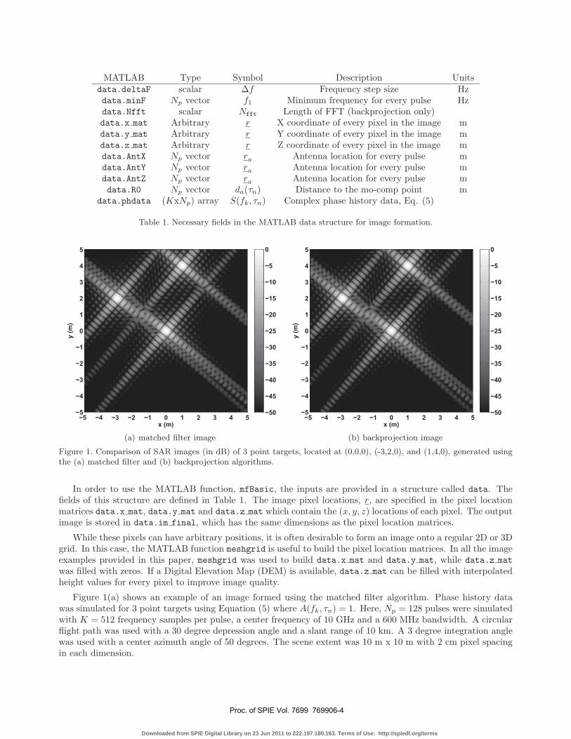
MATLAB Type Symbol Description Unitsdata.deltaF scalar Δf Frequency step size Hzdata.minF Np vector f1 Minimum frequency for every pulse Hzdata.Nfft scalar Nfft Length of FFT (backprojection only)data.x mat Arbitrary r X coordinate of every pixel in the image mdata.y mat Arbitrary r Y coordinate of every pixel in the image mdata.z mat Arbitrary r Z coordinate of every pixel in the image mdata.AntX Np vector ra Antenna location for every pulse mdata.AntY Np vector ra Antenna location for every pulse mdata.AntZ Np vector ra Antenna location for every pulse mdata.R0 Np vector da(τn) Distance to the mo-comp point m

data.phdata (KxNp) array S(fk, τn) Complex phase history data, Eq. (5)

Table 1. Necessary fields in the MATLAB data structure for image formation.

x (m)

y (m

)

−5 −4 −3 −2 −1 0 1 2 3 4 5−5

−4

−3

−2

−1

0

1

2

3

4

5

−50

−45

−40

−35

−30

−25

−20

−15

−10

−5

0

(a) matched filter image

x (m)

y (m

)

−5 −4 −3 −2 −1 0 1 2 3 4 5−5

−4

−3

−2

−1

0

1

2

3

4

5

−50

−45

−40

−35

−30

−25

−20

−15

−10

−5

0

(b) backprojection image

Figure 1. Comparison of SAR images (in dB) of 3 point targets, located at (0,0,0), (-3,2,0), and (1,4,0), generated usingthe (a) matched filter and (b) backprojection algorithms.

In order to use the MATLAB function, mfBasic, the inputs are provided in a structure called data. Thefields of this structure are defined in Table 1. The image pixel locations, r, are specified in the pixel locationmatrices data.x mat, data.y mat and data.z mat which contain the (x, y, z) locations of each pixel. The outputimage is stored in data.im final, which has the same dimensions as the pixel location matrices.

While these pixels can have arbitrary positions, it is often desirable to form an image onto a regular 2D or 3Dgrid. In this case, the MATLAB function meshgrid is useful to build the pixel location matrices. In all the imageexamples provided in this paper, meshgrid was used to build data.x mat and data.y mat, while data.z mat

was filled with zeros. If a Digital Elevation Map (DEM) is available, data.z mat can be filled with interpolatedheight values for every pixel to improve image quality.

Figure 1(a) shows an example of an image formed using the matched filter algorithm. Phase history datawas simulated for 3 point targets using Equation (5) where A(fk, τn) = 1. Here, Np = 128 pulses were simulatedwith K = 512 frequency samples per pulse, a center frequency of 10 GHz and a 600 MHz bandwidth. A circularflight path was used with a 30 degree depression angle and a slant range of 10 km. A 3 degree integration anglewas used with a center azimuth angle of 50 degrees. The scene extent was 10 m x 10 m with 2 cm pixel spacingin each dimension.



4. BACKPROJECTION ALGORITHM

The backprojection algorithm offers an intuitive imaging technique for SAR novices. While the backprojectionalgorithm is computationally expensive, its implementation is not unreasonable for many SAR research ventures.In this section, backprojection imaging equations are manipulated in order to illustrate how the algorithm canbe executed through use of common MATLAB functions.

4.1 Derivation of Efficient Calculation of Range Profiles

The matched filter response shown in Equation (11) can be used to compute the target response at a discreterange bin, m. Given SAR phase history, S(fk, τn), collected by Np pulses over a range of K frequencies, therange profile at range bin m given a received pulse at slow time τn is

s(m, τn) =K∑

k=1

S(fk, τn) exp

(+j4πfkΔR(m, τn)

c

). (12)

By substituting the frequency values fk = (k− 1)Δf + f1 into Equation (12), the range profile may be rewrittenas

s(m, τn) =K∑

k=1

S(fk, τn) exp

(+j4π((k − 1)Δf + f1)ΔR(m, τn)

c

)

=K∑

k=1

S(fk, τn) exp

(+j4πΔfΔR(m, τn)(k − 1)

c+

+j4πf1ΔR(m, τn)

c

)

=K∑

k=1

S(fk, τn) exp[Φ(ΔR(m, τn)) · (k − 1)] exp

(+j4πf1ΔR(m, τn)

c

)(13)

where phase function Φ(ΔR(m, τn)) = (+j4πΔfΔR(m, τn))/c.

In order to implement the backprojection algorithm in MATLAB, Equation (13) must be rewritten in termsof MATLAB’s inverse discrete Fourier transform (ifft) function. In MATLAB, the definitions of the discreteFourier transforms between X(k) and x(m) are given as19

X(k) =M∑

m=1

x(m) · ω(m−1)(k−1)K

x(m) =1

K

K∑k=1

X(k) · ω−(m−1)(k−1)K

(14)

where ωK = exp(−j2π/K). Therefore, the inverse discrete Fourier transform of X(k) is given as

x(m) = ifft(X(k)) =1

K

K∑k=1

X(k) exp

(+j2π(m− 1)

K· (k − 1)

)=

1

K

K∑k=1

X(k) exp (Θ(m) · (k − 1)) (15)

where Θ(m) = (j2π(m − 1))/K. In order to write Equation (13) in terms of MATLAB’s ifft function, thepreviously defined phase function, Φ(ΔR(m, τn)), from Equation(13), must equal Θ(m) from Equation (15). Tosatisfy this requirement, the following equality must hold:

ΔR(m, τn) =(m− 1)

K· c

2Δf=

(m− 1)

K·Wr. (16)

Note that ΔR(m, τn) represents a sampling across range and the maximum unambiguous range occurs when(m− 1) = K (recall Equation (7)).



Inserting the result from Equation (16) into Equation (13) yields

s(m, τn) =

K∑k=1

S(fk, τn) exp

(+j4πΔf(k − 1)

c·ΔR(m, τn)

)· exp

(+j4πf1ΔR(m, τn)

c

)

=

K∑k=1

S(fk, τn) exp

(+j4πΔf(k − 1)

c·(m− 1

K· c

2Δf

))· exp

(+j4πf1ΔR(m, τn)

c

)

=

K∑k=1

S(fk, τn) exp

(+j2π(m− 1)

K· (k − 1)

)· exp

(+j4πf1ΔR(m, τn)

c

).

(17)

Finally, recalling the expression for the inverse discrete Fourier transform from Equation (15), the range profilemay be expressed in terms of MATLAB’s ifft.

s(m, τn) = K · ifft(S(fk, τn)) · exp(+j4πf1ΔR(m, τn)

c

)(18)

The constant K appears in Equation (18) because by definition, the inverse discrete Fourier transform con-tains a scaling factor of 1/K. In addition, it’s important to note that the MATLAB implementation of theinverse discrete Fourier transform assumes that K is even. However, for values of K that are powers of 2, thecomputational complexity of the inverse discrete Fourier transform is optimized. By inserting the expression forΔR(m, τn) from Equation (16), an alternative expression for the implementation of a range profile in MATLABis given by

s(m, τn) = K · ifft(S(fk, τn)) · exp(j2πf1(m− 1)

KΔf

). (19)

One final consideration must be addressed. Each pulse is motion compensated such that a scatterer at thescene origin has zero phase and will appear in the zero frequency bin in the range profile. This bin correspondsto the center of the range profile computed in Equation (19). By default, the function ifft computes the valuesfrom 1 ≤ m ≤ K where m = 1 corresponds to the zero frequency bin. To put m = 1 at the center of the rangeprofile, the command fftshift is applied to the output of the ifft command. This operation ensures that theoutput is correctly ordered following the inverse discrete Fourier transform operation and that the zero frequencycomponent corresponds to the center of the output vector.

As a result, range index, m, acquires values between −K/2 + 1 and K/2. Therefore, ΔR(m, τn) of Equation(16) has values between −Wr/2 and Wr/2−Wr/K and Equation (19) becomes

s(m, τn) = K · fftshift{ifft(S(fk, τn))} · exp(j2πf1(m− 1)

KΔf

). (20)

4.2 Image Formation Process

For implementation of the backprojection imaging algorithm in MATLAB, Equation (6) is used to compute thedifferential range, ΔR(τn), for each pixel, for each pulse, where the pixel (x, y, z) coordinates are inserted intoEquation (4). In order to use Equation (20) to form a SAR image, an interpolation step is required due tothe fact that the discrete values of ΔR(m, τn) do not correspond exactly to the ΔR(τn) values calculated forevery pixel. There are several methods for performing this interpolation,20,11 but here we will simply use theMATLAB interp1 function to implement linear interpolation.

Since s(m, τn) is a band-limited signal, the ideal interpolator is a sinc interpolator. This can be approximatedby zero-padding the ifft computation and then performing linear interpolation on the inverse discrete Fouriertransform output. A good rule of thumb is that the length of the ifft, denoted Nfft, should be 10 times thelength of the data, K. Also, the ifft function is most efficient when Nfft is a power of 2. In the backprojectionalgorithm, Nfft is provided as an input to the imaging function, as shown in Table 1.



The first step in the image formation process is to implement Equation (20) for every pulse, zero-paddingthe data such that the length of the ifft is Nfft. Thus,

s(m, τn) = Nfft · fftshift{ifft(S(fk, τn))} · exp(j2πf1(m− 1)

NfftΔf

). (21)

where S(fk, τn) = 0 for all k > K.

To find the image response for a pixel at location r, given pulse n, ΔR(τn) is calculated and used to findan interpolated value of s(m, τn). This is denoted as sint(r, τn). The final image response, I(r), is simply thesummation of these values for every pulse.

I(r) =

Np∑n=1

sint(r, τn). (22)

Figure 1(b) shows an example of an image formed using the backprojection algorithm. The image wasgenerated using the same data and equivalent pixel locations as those employed in Figure 1(a).

5. IMAGE EXAMPLES

In the last few years, the Air Force Research Laboratory (AFRL) has released several datasets of both syntheticand measured SAR data. In this section, the backprojection algorithm introduced in Section 4 is applied to datafrom the Backhoe Data Dome, the 2D/3D Volumetric Challenge Problem, and the SAR-based Ground MovingTarget Indicator (GMTI) Challenge Problem. In addition, the imaging code was implemented on the CivilianVehicle Radar Data Domes synthetic data set from The Ohio State University.

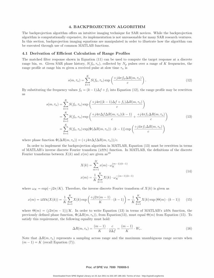
5.1 Backhoe Data Dome

In 2004, AFRL released a synthetically generated data dome of a backhoe target.21 The scattered field data forthe backhoe was computed on a 2π-steradian data dome over the target for a frequency bandwidth of 5.9 GHzat a center frequency of 10 GHz.

x (m)

y (m

)

−5 −4 −3 −2 −1 0 1 2 3 4 5−5

−4

−3

−2

−1

0

1

2

3

4

5

−70

−60

−50

−40

−30

−20

−10

0

Figure 2. Backprojection image (in dB) using the Backhoe Data Dome synthetic dataset.

The backprojection algorithm was performed on this dataset and a resulting image is given in Figure 2. Thedata imaged consisted of all 360◦ aspect angles from a single elevation of 10◦ using VV polarization. The full 5.9GHz bandwidth was used to form the image. The scene extent is 10 m x 10 m with 2 cm pixel spacing, resultingin a 501 x 501 pixel image. No windowing was applied to the data before imaging. The calculated maximumscene size is Wr = 12.97 m; Wx = 9.27 m.



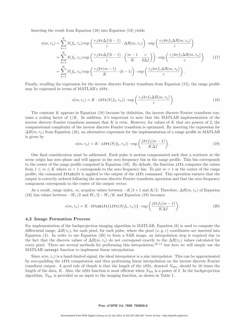
5.2 2D/3D Volumetric Challenge Problem

In 2007, AFRL released a challenge problem for 2D/3D imaging of targets from a volumetric data set in anurban environment.22 The data was collected of a scene consisting of numerous civilian vehicles and calibrationtargets.

The backprojection algorithm was performed on this dataset and a resulting image is given in Figure 3. Thedata imaged consisted of Pass 1 with HH polarization. An integration angle, Δθ, of 4◦ centered at 40◦ azimuthwas used. The scene extent is 100 m x 100 m with 20 cm pixel spacing, resulting in a 501 x 501 pixel image.No windowing was applied to the data before imaging. The calculated maximum scene size is Wr = 101.87 m;Wx = 108.41 m and the calculated resolution is δr = 0.24 m; δx = 0.23 m.

x (m)

y (m

)

−50 −25 0 25 50−50

−25

0

25

50

−70

−60

−50

−40

−30

−20

−10

0

Figure 3. Backprojection image (in dB) using the 2D/3D Volumetric Challenge Problem dataset.

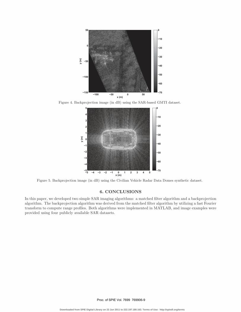
5.3 SAR-based GMTI Challenge Problem

In 2009, AFRL released a challenge problem for SAR-based GMTI in urban environments.23 This data consistsof a 71-second portion of phase history data from a radar operating in circular SAR mode. The data hasbeen range-gated around the known location of a moving vehicle, severely limiting the range swath of the data.However, during the first 25 seconds of the scenario, the vehicle is waiting in line to cross a busy intersection.

The backprojection algorithm was performed on this dataset and a resulting image is provided in Figure4. The scene extent is 200 m x 200 m with 20 cm pixel spacing, resulting in a 1001 x 1001 pixel image. Thefirst 8000 pulses (almost 4 seconds) were used, and no windowing was applied to the data before imaging. Thecalculated maximum scene size is Wr = 89.94 m; Wx = 2, 032.41 m, and the calculated resolution is δr = 0.23m; δx = 0.25 m. The relatively small range extent accounts for the black areas in the image.

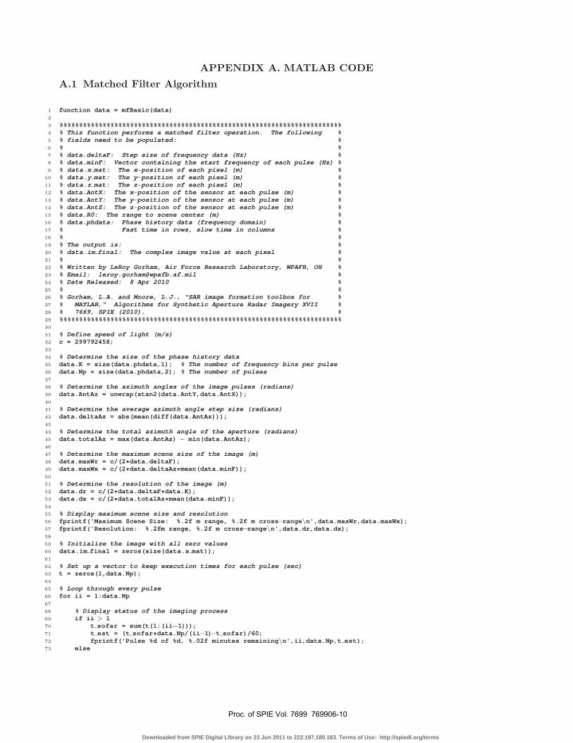
5.4 Civilian Vehicle Radar Data Domes

In 2010, The Ohio State University released a set of synthetically generated data domes of civilian targets.24

The scattered field data for the targets was computed for full azimuth coverage of elevation angles from 30◦ to60◦. The data is full polarimetric with a frequency bandwidth of 5.35 GHz at a center frequency of 9.6 GHz.

The backprojection algorithm was implemented on the 1993 Jeep target, and a resulting image is shown inFigure 5. The data imaged consisted of all 360◦ aspect angles from a single elevation of 30◦ using VV polarization.The full bandwidth was used to form the image. The scene extent is 10 m x 10 m with 2 cm pixel spacing,resulting in a 501 x 501 pixel image. No windowing was applied to the data before imaging. The calculatedmaximum scene size is Wr = 14.30 m; Wx = 11.18 m.



x (m)

y (m

)

−100 −50 0 50−150

−100

−50

0

50

−70

−60

−50

−40

−30

−20

−10

0

Figure 4. Backprojection image (in dB) using the SAR-based GMTI dataset.

x (m)

y (m

)

−5 −4 −3 −2 −1 0 1 2 3 4 5−5

−4

−3

−2

−1

0

1

2

3

4

5

−70

−60

−50

−40

−30

−20

−10

0

Figure 5. Backprojection image (in dB) using the Civilian Vehicle Radar Data Domes synthetic dataset.

6. CONCLUSIONS

In this paper, we developed two simple SAR imaging algorithms: a matched filter algorithm and a backprojectionalgorithm. The backprojection algorithm was derived from the matched filter algorithm by utilizing a fast Fouriertransform to compute range profiles. Both algorithms were implemented in MATLAB, and image examples wereprovided using four publicly available SAR datasets.



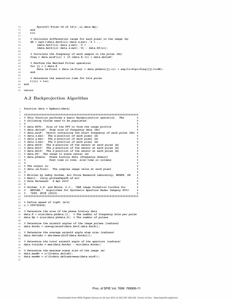
APPENDIX A. MATLAB CODE

A.1 Matched Filter Algorithm

1 function data = mfBasic(data)2

3 %%%%%%%%%%%%%%%%%%%%%%%%%%%%%%%%%%%%%%%%%%%%%%%%%%%%%%%%%%%%%%%%%%%%%%%%4 % This function performs a matched filter operation. The following %5 % fields need to be populated: %6 % %7 % data.deltaF: Step size of frequency data (Hz) %8 % data.minF: Vector containing the start frequency of each pulse (Hz) %9 % data.x mat: The x−position of each pixel (m) %

10 % data.y mat: The y−position of each pixel (m) %11 % data.z mat: The z−position of each pixel (m) %12 % data.AntX: The x−position of the sensor at each pulse (m) %13 % data.AntY: The y−position of the sensor at each pulse (m) %14 % data.AntZ: The z−position of the sensor at each pulse (m) %15 % data.R0: The range to scene center (m) %16 % data.phdata: Phase history data (frequency domain) %17 % Fast time in rows, slow time in columns %18 % %19 % The output is: %20 % data.im final: The complex image value at each pixel %21 % %22 % Written by LeRoy Gorham, Air Force Research Laboratory, WPAFB, OH %23 % Email: [email protected] %24 % Date Released: 8 Apr 2010 %25 % %26 % Gorham, L.A. and Moore, L.J., "SAR image formation toolbox for %27 % MATLAB," Algorithms for Synthetic Aperture Radar Imagery XVII %28 % 7669, SPIE (2010). %29 %%%%%%%%%%%%%%%%%%%%%%%%%%%%%%%%%%%%%%%%%%%%%%%%%%%%%%%%%%%%%%%%%%%%%%%%30

31 % Define speed of light (m/s)32 c = 299792458;33

34 % Determine the size of the phase history data35 data.K = size(data.phdata,1); % The number of frequency bins per pulse36 data.Np = size(data.phdata,2); % The number of pulses37

38 % Determine the azimuth angles of the image pulses (radians)39 data.AntAz = unwrap(atan2(data.AntY,data.AntX));40

41 % Determine the average azimuth angle step size (radians)42 data.deltaAz = abs(mean(diff(data.AntAz)));43

44 % Determine the total azimuth angle of the aperture (radians)45 data.totalAz = max(data.AntAz) − min(data.AntAz);46

47 % Determine the maximum scene size of the image (m)48 data.maxWr = c/(2*data.deltaF);49 data.maxWx = c/(2*data.deltaAz*mean(data.minF));50

51 % Determine the resolution of the image (m)52 data.dr = c/(2*data.deltaF*data.K);53 data.dx = c/(2*data.totalAz*mean(data.minF));54

55 % Display maximum scene size and resolution56 fprintf('Maximum Scene Size: %.2f m range, %.2f m cross−range\n',data.maxWr,data.maxWx);57 fprintf('Resolution: %.2fm range, %.2f m cross−range\n',data.dr,data.dx);58

59 % Initialize the image with all zero values60 data.im final = zeros(size(data.x mat));61

62 % Set up a vector to keep execution times for each pulse (sec)63 t = zeros(1,data.Np);64

65 % Loop through every pulse66 for ii = 1:data.Np67

68 % Display status of the imaging process69 if ii > 170 t sofar = sum(t(1:(ii−1)));71 t est = (t sofar*data.Np/(ii−1)−t sofar)/60;72 fprintf('Pulse %d of %d, %.02f minutes remaining\n',ii,data.Np,t est);73 else

Proc. of SPIE Vol. 7699 769906-10


74 fprintf('Pulse %d of %d\n',ii,data.Np);75 end76 tic77

78 % Calculate differential range for each pixel in the image (m)79 dR = sqrt((data.AntX(ii)−data.x mat).ˆ2 + ...80 (data.AntY(ii)−data.y mat).ˆ2 + ...81 (data.AntZ(ii)−data.z mat).ˆ2) − data.R0(ii);82

83 % Calculate the frequency of each sample in the pulse (Hz)84 freq = data.minF(ii) + (0:(data.K−1)) * data.deltaF;85

86 % Perform the Matched Filter operation87 for jj = 1:data.K88 data.im final = data.im final + data.phdata(jj,ii) * exp(1i*4*pi*freq(jj)/c*dR);89 end90

91 % Determine the execution time for this pulse92 t(ii) = toc;93 end94

95 return

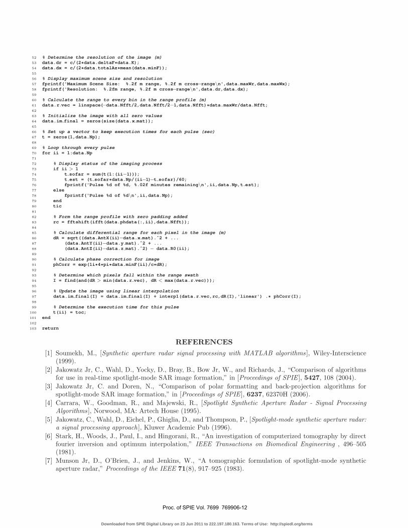
A.2 Backprojection Algorithm

1 function data = bpBasic(data)2

3 %%%%%%%%%%%%%%%%%%%%%%%%%%%%%%%%%%%%%%%%%%%%%%%%%%%%%%%%%%%%%%%%%%%%%%%%4 % This function performs a basic Backprojection operation. The %5 % following fields need to be populated: %6 % %7 % data.Nfft: Size of the FFT to form the range profile %8 % data.deltaF: Step size of frequency data (Hz) %9 % data.minF: Vector containing the start frequency of each pulse (Hz) %

10 % data.x mat: The x−position of each pixel (m) %11 % data.y mat: The y−position of each pixel (m) %12 % data.z mat: The z−position of each pixel (m) %13 % data.AntX: The x−position of the sensor at each pulse (m) %14 % data.AntY: The y−position of the sensor at each pulse (m) %15 % data.AntZ: The z−position of the sensor at each pulse (m) %16 % data.R0: The range to scene center (m) %17 % data.phdata: Phase history data (frequency domain) %18 % Fast time in rows, slow time in columns %19 % %20 % The output is: %21 % data.im final: The complex image value at each pixel %22 % %23 % Written by LeRoy Gorham, Air Force Research Laboratory, WPAFB, OH %24 % Email: [email protected] %25 % Date Released: 8 Apr 2010 %26 % %27 % Gorham, L.A. and Moore, L.J., "SAR image formation toolbox for %28 % MATLAB," Algorithms for Synthetic Aperture Radar Imagery XVII %29 % 7669, SPIE (2010). %30 %%%%%%%%%%%%%%%%%%%%%%%%%%%%%%%%%%%%%%%%%%%%%%%%%%%%%%%%%%%%%%%%%%%%%%%%31

32 % Define speed of light (m/s)33 c = 299792458;34

35 % Determine the size of the phase history data36 data.K = size(data.phdata,1); % The number of frequency bins per pulse37 data.Np = size(data.phdata,2); % The number of pulses38

39 % Determine the azimuth angles of the image pulses (radians)40 data.AntAz = unwrap(atan2(data.AntY,data.AntX));41

42 % Determine the average azimuth angle step size (radians)43 data.deltaAz = abs(mean(diff(data.AntAz)));44

45 % Determine the total azimuth angle of the aperture (radians)46 data.totalAz = max(data.AntAz) − min(data.AntAz);47

48 % Determine the maximum scene size of the image (m)49 data.maxWr = c/(2*data.deltaF);50 data.maxWx = c/(2*data.deltaAz*mean(data.minF));51

Proc. of SPIE Vol. 7699 769906-11


52 % Determine the resolution of the image (m)53 data.dr = c/(2*data.deltaF*data.K);54 data.dx = c/(2*data.totalAz*mean(data.minF));55

56 % Display maximum scene size and resolution57 fprintf('Maximum Scene Size: %.2f m range, %.2f m cross−range\n',data.maxWr,data.maxWx);58 fprintf('Resolution: %.2fm range, %.2f m cross−range\n',data.dr,data.dx);59

60 % Calculate the range to every bin in the range profile (m)61 data.r vec = linspace(−data.Nfft/2,data.Nfft/2−1,data.Nfft)*data.maxWr/data.Nfft;62

63 % Initialize the image with all zero values64 data.im final = zeros(size(data.x mat));65

66 % Set up a vector to keep execution times for each pulse (sec)67 t = zeros(1,data.Np);68

69 % Loop through every pulse70 for ii = 1:data.Np71

72 % Display status of the imaging process73 if ii > 174 t sofar = sum(t(1:(ii−1)));75 t est = (t sofar*data.Np/(ii−1)−t sofar)/60;76 fprintf('Pulse %d of %d, %.02f minutes remaining\n',ii,data.Np,t est);77 else78 fprintf('Pulse %d of %d\n',ii,data.Np);79 end80 tic81

82 % Form the range profile with zero padding added83 rc = fftshift(ifft(data.phdata(:,ii),data.Nfft));84

85 % Calculate differential range for each pixel in the image (m)86 dR = sqrt((data.AntX(ii)−data.x mat).ˆ2 + ...87 (data.AntY(ii)−data.y mat).ˆ2 + ...88 (data.AntZ(ii)−data.z mat).ˆ2) − data.R0(ii);89

90 % Calculate phase correction for image91 phCorr = exp(1i*4*pi*data.minF(ii)/c*dR);92

93 % Determine which pixels fall within the range swath94 I = find(and(dR > min(data.r vec), dR < max(data.r vec)));95

96 % Update the image using linear interpolation97 data.im final(I) = data.im final(I) + interp1(data.r vec,rc,dR(I),'linear') .* phCorr(I);98

99 % Determine the execution time for this pulse100 t(ii) = toc;101 end102

103 return

REFERENCES

[1] Soumekh, M., [Synthetic aperture radar signal processing with MATLAB algorithms ], Wiley-Interscience(1999).

[2] Jakowatz Jr, C., Wahl, D., Yocky, D., Bray, B., Bow Jr, W., and Richards, J., “Comparison of algorithmsfor use in real-time spotlight-mode SAR image formation,” in [Proceedings of SPIE ], 5427, 108 (2004).

[3] Jakowatz Jr, C. and Doren, N., “Comparison of polar formatting and back-projection algorithms forspotlight-mode SAR image formation,” in [Proceedings of SPIE ], 6237, 62370H (2006).

[4] Carrara, W., Goodman, R., and Majewski, R., [Spotlight Synthetic Aperture Radar - Signal ProcessingAlgorithms ], Norwood, MA: Artech House (1995).

[5] Jakowatz, C., Wahl, D., Eichel, P., Ghiglia, D., and Thompson, P., [Spotlight-mode synthetic aperture radar:a signal processing approach ], Kluwer Academic Pub (1996).

[6] Stark, H., Woods, J., Paul, I., and Hingorani, R., “An investigation of computerized tomography by directfourier inversion and optimum interpolation,” IEEE Transactions on Biomedical Engineering , 496–505(1981).

[7] Munson Jr, D., O’Brien, J., and Jenkins, W., “A tomographic formulation of spotlight-mode syntheticaperture radar,” Proceedings of the IEEE 71(8), 917–925 (1983).

Proc. of SPIE Vol. 7699 769906-12


[8] Gorham, L. A., Rigling, B. D., and Zelnio, E. G., “A comparison between imaging radar and medicalimaging polar format algorithm implementations,” in [Proceedings of SPIE ], 6568, 65680K (2007).

[9] Doren, N., Jakowatz Jr, C., Wahl, D., and Thompson, P., “General formulation for wavefront curvaturecorrection in polar-formatted spotlight-mode SAR images using space-variant post-filtering,” in [Proceedingsof the 1997 International Conference on Image Processing (ICIP’97) 3-Volume Set-Volume 1-Volume 1 ],IEEE Computer Society Washington, DC, USA (1997).

[10] Preiss, M., Gray, D., and Stacy, N., “Space Variant Filtering of Polar Format Spotlight SAR Images forWavefront Curvature Correction and Interferometric Processing,” in [IGARSS 2002: IEEE InternationalGeoscience and Remote Sensing Symposium (24th: 2002: Toronto, Ontario) ], IEEE: Institute of Electricaland Electronics Engineers (2002).

[11] Desai, M. and Jenkins, W., “Convolution backprojection image reconstruction for spotlight mode syntheticaperture radar,” IEEE Transactions on Image Processing 1(4), 505–517 (1992).

[12] Hartley, T., Fasih, A., Berdanier, C., Ozguner, F., and Catalyurek, U., “Investigating the use of GPU-accelerated nodes for SAR image formation,” in [Cluster Computing and Workshops, 2009. CLUSTER ’09.IEEE International Conference on ], 1–8 (Aug 31–Sep 4 2009).

[13] Rogan, A. and Carande, R., “Improving the fast backprojection algorithm through massive parallelizations,”Radar Sensor Technology XIV 7669(1), SPIE (2010).

[14] Yegulalp, A., “Fast backprojection algorithm for synthetic aperture radar,” in [Radar Conference, 1999.The Record of the 1999 IEEE ], 60–65 (1999).

[15] McCorkle, J. and Rofheart, M., “An order N2log(N) backprojector algorithm for focusing wide-angle wide-bandwidth arbitrary-motion synthetic aperture radar,” in [Proc. of SPIE Conference on Radar SensorTechnology ], 2747, 25–36 (1996).

[16] Ulander, L., Hellsten, H., and Stenstrom, G., “Synthetic-aperture radar processing using fast factorizedback-projection,” IEEE Transactions on Aerospace and electronic systems 39(3), 760–776 (2003).

[17] Wahl, D. E., Yocky, D. A., and Jakowatz Jr., C. V., “An implementation of a fast backprojection imageformation algorithm for spotlight-mode SAR,” in [Proceedings of SPIE ], 6970, 69700H (2008).

[18] Rigling, B. and Moses, R., “Taylor expansion of the differential range for monostatic SAR,” IEEE Trans-actions on Aerospace and Electronic Systems 41(1), 60–64 (2005).

[19] The Mathworks, Inc, MATLAB Documentation: fft - Discrete Fourier Transform. Version 7.9.0.529(R2009b).

[20] Crochiere, R. and Rabiner, L., “Interpolation and decimation of digital signals - a tutorial review,” Pro-ceedings of the IEEE 69(3), 300–331 (1981).

[21] Naidu, K. and Lin, L., “Data dome: full k-space sampling data for high-frequency radar research,” Algo-rithms for Synthetic Aperture Radar Imagery XI 5427(1), 200–207, SPIE (2004).

[22] Casteel Jr, C. H., Gorham, L. A., Minardi, M. J., Scarborough, S. M., Naidu, K. D., and Majumder, U. K.,“A challenge problem for 2D/3D imaging of targets from a volumetric data set in an urban environment,”Algorithms for Synthetic Aperture Radar Imagery XIV 6568(1), 65680D, SPIE (2007).

[23] Scarborough, S. M., Casteel Jr, C. H., Gorham, L., Minardi, M. J., Majumder, U. K., Judge, M. G.,Zelnio, E., Bryant, M., Nichols, H., and Page, D., “A challenge problem for SAR-based GMTI in urbanenvironments,” Algorithms for Synthetic Aperture Radar Imagery XVI 7337(1), 73370G, SPIE (2009).

[24] Dungan, K. E., Austin, C., Nehrbass, J., and Potter, L. C., “Civilian vehicle radar data domes,” Algorithmsfor Synthetic Aperture Radar Imagery XVII 7699(1), SPIE (2010).

Proc. of SPIE Vol. 7699 769906-13


SAR image formation toolbox for MATLAB -...

Documents

Transcript of SAR image formation toolbox for MATLAB -...