SANDIA REPORT SAND2014-0369 Unlimited Release Printed January 2014

SAR Image Effects on Coherence and Coherence Estimation Douglas L. Bickel Prepared by Sandia National Laboratories Albuquerque, New Mexico 87185 and Livermore, California 94550

Sandia National Laboratories is a multi-program laboratory managed and operated by Sandia Corporation, a wholly owned subsidiary of Lockheed Martin Corporation, for the U.S. Department of Energy's National Nuclear Security Administration under contract DE-AC04-94AL85000.

Approved for public release; further dissemination unlimited.

Issued by Sandia National Laboratories, operated for the United States Department of Energy by Sandia Corporation. NOTICE: This report was prepared as an account of work sponsored by an agency of the United States Government. Neither the United States Government, nor any agency thereof, nor any of their employees, nor any of their contractors, subcontractors, or their employees, make any warranty, express or implied, or assume any legal liability or responsibility for the accuracy, completeness, or usefulness of any information, apparatus, product, or process disclosed, or represent that its use would not infringe privately owned rights. Reference herein to any specific commercial product, process, or service by trade name, trademark, manufacturer, or otherwise, does not necessarily constitute or imply its endorsement, recommendation, or favoring by the United States Government, any agency thereof, or any of their contractors or subcontractors. The views and opinions expressed herein do not necessarily state or reflect those of the United States Government, any agency thereof, or any of their contractors. Printed in the United States of America. This report has been reproduced directly from the best available copy. Available to DOE and DOE contractors from U.S. Department of Energy Office of Scientific and Technical Information P.O. Box 62 Oak Ridge, TN 37831 Telephone: (865) 576-8401 Facsimile: (865) 576-5728 E-Mail: reports@adonis.osti.gov Online ordering: http://www.osti.gov/bridge Available to the public from U.S. Department of Commerce National Technical Information Service 5285 Port Royal Rd. Springfield, VA 22161 Telephone: (800) 553-6847 Facsimile: (703) 605-6900 E-Mail: orders@ntis.fedworld.gov Online order: http://www.ntis.gov/help/ordermethods.asp?loc=7-4-0#online

SAND2014-0369 Unclassified Unlimited Release

Printed January 2014

SAR Image Effects on Coherence and Coherence Estimation

Douglas L. Bickel

ISR Analysis and Application Sandia National Laboratories

PO Box 5800 Albuquerque, NM 87185

ABSTRACT Radar coherence is an important concept for imaging radar systems such as synthetic aperture radar (SAR). This document quantifies some of the effects in SAR which modify the coherence. Although these effects can disrupt the coherence within a single SAR image, this report will focus on the coherence between separate images, such as for coherent change detection (CCD) processing. There have been other presentations on aspects of this material in the past. The intent of this report is to bring various issues that affect the coherence together in a single report to support radar engineers in making decisions about these matters.

- 3 -

ACKNOWLEDGEMENTS

The author would like to acknowledge the code provided by, and valuable discussions with Dr. Rick Naething of Sandia National Laboratories on the subject of interpolation and coherence. The author also appreciates the helpful discussions on this same subject with Dr. Richard Bamler of the DLR.

Sandia National Laboratories is a multi-program laboratory managed and operated by Sandia Corporation, a wholly owned subsidiary of Lockheed Martin Corporation, for the U.S. Department of Energy’s National Nuclear Security Administration under contract DE-AC04-94AL85000.

- 4 -

CONTENTS ABSTRACT ........................................................................................................................ 3

1. Executive Summary .................................................................................................. 7

2. Introduction ............................................................................................................... 9

3. Coherence basics ..................................................................................................... 10

4. Coherence loss ........................................................................................................ 13

5. Estimation of coherence .......................................................................................... 39

6. Conclusions ............................................................................................................. 50

8. References ............................................................................................................... 51

9. Appendix A: Symbols and terminology ................................................................ 52

10. Distribution ............................................................................................................. 54

- 5 -

This page left intentionally blank.

- 6 -

1. Executive Summary This report attempts to pull together equations concerning coherence between synthetic aperture radar images. Various error sources between images and their effects on the coherence between the images are presented. Also examined are equations pertaining to the estimation of coherence, including bias and variance. The purpose of this document is to assist radar engineers in understanding assorted coherence issues with application to coherent change detection.

- 7 -

This page left intentionally blank.

- 8 -

2. Introduction Radar coherence is an important concept for imaging radar systems such as synthetic aperture radar (SAR). This document quantifies some of the effects in SAR which modify the coherence. Although these effects can disrupt the coherence within a single SAR image, this report will focus on the coherence between separate images, such as for coherent change detection (CCD) processing. There have been other presentations on aspects of this material in the past. The intent of this report is to bring various issues that affect the coherence together in a single report.

The reader is assumed to have basic familiarity with the concepts of radar coherence. Although the concepts presented in this document are general, the emphasis of this document will be on the CCD application of radar coherence. In particular, the focus is on detection of man-made temporal changes in the coherence; therefore, all other causes of decorrelation are assumed to be a nuisance.

The outline of this report is now presented. Section 3 gives a very brief overview of coherence. This section will also present some of the assumptions used throughout the report. Section 4 discusses sources of coherence loss and presents equations and analysis of various sources of loss. The final section will discuss estimation of coherence given radar data and attributes of the estimators. This report then ends with a brief overview in the conclusions section.

- 9 -

3. Coherence basics It will be assumed in this report that the reader has a good basic understanding of coherence as it applies to CCD [4] or the similar concept of interferometric SAR (IFSAR) [1,4]. Therefore, this section will only briefly highlight a few concepts which are key to this report.

Some basic assumptions that pertain to this report are now discussed. First, for the CCD application we are concerned with coherence between images, rather than between pulses. The effect of the latter on the former is discussed in a follow-on section. Next, we are concerned with coherence of natural clutter, or distributed targets1. For this case, we will make the standard assumptions of circularly Gaussian statistics for both clutter and noise. We assume that the statistics are stationary over the regions of interest. Essentially, radar clutter is assumed to behave like an incoherent source in optics [6]. Another assumption is that imaging geometries in this report are broadside.

A few interesting observations are discussed here to attempt to illuminate some of the implications of modeling clutter as an incoherent source. First, under some specific simplifying assumptions, (i.e., sinc function impulse response, proper sampling, etc.) this model of clutter leads to the practical statement that in natural clutter, adjacent resolution cells are uncorrelated. Second, and again based upon this model, if we image the same clutter area from non-overlapped spatial frequency bands, the images will be statistically independent of each other. This occurs when clutter is observed from differing geometries. This latter fact is important and will be discussed more later on in this report. As an example, images from non-overlapped aperture angles can be used for speckle reduction techniques in traditional image processing. Finally, it is important to notice that uncorrelated clutter has the same model as thermal noise. Since uncorrelated clutter has the same power as correlated clutter, sources of clutter decorrelation can often be more important that thermal noise effects.

The definition of the coherence for complex data is given by:

( ) ( )1 2

1 1 2 2

0x x

x x x xµ

σ σ

∗− −

= (1)

where: is the expectation operator

1x , 2x - are the pixels from the two images being correlated, image 1 and 2, respectively

ixσ - is the square-root of the variance for the pixel from the ith image

1 As pointed out in [4], point and/or specular targets have different coherence behavior than distributed clutter.

- 10 -

In general, we assume that clutter is zero-mean, so we can rewrite equation (1) as:

1 20 2 2

1 2

x x

x xµ

∗

= (2)

Also, for the CCD application, we tend to be interested in the magnitude of equation (2). We will use 0µ as the magnitude of equation and only use 0µ when it adds clarity to the discussion. The estimator for the expectation in equation (2) is presented later in this document.

The resulting CCD product can be thought of as several decorrelation terms, e.g., 1d and

2d , and a correlated term, c , remaining after all of the decorrelation. The decorrelation terms can be due to various sources of which many will be mentioned later in this section. The coherence in this case can be written as the ratio of the correlated term to the total:

1 2

cc d d

µ =+ +

(3)

If there is only decorrelation due to the 1d source, then the coherence is:

1 21

1 1 1 2

c c dc d c d d

µ +

= = + + + (4)

In other words, 2d has not caused decorrelation yet.

Now if another decorrelation source, 2d , acts upon the residual correlated part of equation (4), 1c , such that the only correlation remaining is c , then we have that the correlation from this source is:

22

cc d

µ =+

(5)

From the previous three equations we see that the final coherence cascades as a product of the individual coherences from the various decorrelation sources:

1 2µ µ µ= (6)

- 11 -

Decorrelation between radar images can come from several sources. The two most obvious are thermal noise and temporal decorrelation2. The former is an undesirable fact of life, and the latter is what we wish to observe in CCD. Other decorrelation sources include: differences in observation geometries (spatial errors); uncompensated motion errors; registration errors; processing errors; interpolation errors; impulse response (IPR) mismatch errors; multiplicative noise; polarization mismatch; and errors in the estimator3. It is very important to point out that the coherence can be more sensitive to these error sources than standard SAR magnitude image. Hopefully this will be obvious from later sections of this document.

2 It should be noted that in this document, temporal decorrelation includes both man-made and natural variations in the clutter cells as a function of time. Generally we are interested in the man-made variation, and the natural variation is undesirable. 3 For example, by this I mean performing the averaging over an area that may not be stationary, e.g., have a large terrain variation.

- 12 -

4. Coherence loss 4.1 Overview

The previous section noted that the coherence is made up of the product of coherences due to individual decorrelation sources. Several potential decorrelation sources were mentioned. This section presents the coherence for many of these individual terms.

4.2 Thermal noise

If we assume that the desired signal-to-noise (SNR) is identical between the two images that are being correlated, then the coherence due to thermal noise follows from equation (5), for example:

1snrs snr

s n snrµ = =

+ + (7)

where s is the correlated signal power (image without noise), n is the thermal noise power, and snr is the signal-to-noise ratio of the image pixel. If the signal-to-noise ratios differ between the images due to gain or thermal noise power differences, then the coherence due to thermal noise becomes:

1 2 1 2

1 1 2 2 1 21 1snrs s snr snr

s n s n snr snrµ = =

+ + + + (8)

where the indices indicate the image number. Figure 1 shows a plot of equation (7) where the signal-to-noise ratios are equal. Figure 2 shows the case where the signal-to-noise ratios are different with one varying and the other is fixed at 10 dB.

It is important to note that decorrelation due to thermal noise is always present and is often assumed to be the dominant factor in the coherence value. Ideally, we want the coherence to approach this value. In other words, we want all other factors discussed in this report4 to have a coherence of one.

Often, it is simpler for radar engineers to think in terms of signal-to-noise ratio rather than coherence. Figure 3 shows the equivalent signal-to-noise ratio given the coherence by inverting equation (7).

4With the obvious exception being the desired man-made temporal decorrelation signature in the CCD.

- 13 -

Figure 1: Coherence due to thermal noise when SNRs are equal in the two images

Figure 2: Coherence due to thermal noise when SNRs are unequal in the two images

-10 0 10 20 30 40 500.2

0.3

0.4

0.5

0.6

0.7

0.8

0.9

1

µ snr

SNR (dB)

-10 0 10 20 30 40 500.4

0.5

0.6

0.7

0.8

0.9

1

µ snr

SNR in image #2 (dB)

SNR in image #1 = 10 dB

- 14 -

Figure 3: Equivalent SNR from coherence

4.3 Geometry and collection issues

Collection geometries, in particular differences in collection geometries between images influence the coherence. To a first order, these geometries affect the spectrum of the observed impulse response. Differences in this spectrum between collects introduce decorrelation. A very good discussion of the relationship between spatial frequencies and coherence can be found in [4].

From previous discussion and in [4], the decorrelation can be related to the amount of overlapping spatial frequency content between the two images to the total spatial frequency content. Also, from previous discussion we can treat the non-overlapping part of the spatial frequency content as noise. The result is that the coherence due to geometry differences can be derived similar to equation (8), and is given by:

1 2

fogeom

fo fn fo fn

SS S S S

µ =+ +

(9)

where:

0 0.1 0.2 0.3 0.4 0.5 0.6 0.7 0.8 0.9 1-30

-20

-10

0

10

20

30

SN

Req

uiva

lent

= 1

0log

10( µ

/(1-µ)

) (d

B)

µ

- 15 -

foS is the overlapping area of the spatial frequencies between the two images5

1fnS - is the non-overlapping spatial frequency due to image #1

2fnS - is the non-overlapping spatial frequency due to image #2

In the next two subsections we discuss the effect of cross-track and along-track geometry differences between passes on coherence between images.

4.3.1 “Cross-track” geometry errors

Cross-track geometry errors are what we tend to think of for coherence because of its emphasis in interferometric SAR, namely the so-called “critical baseline”. This error occurs due to the spatial frequency shift from cross-track errors, which comes from observing the two images from differing grazing angles.

Figure 4a and Figure 4b show the spatial frequency for two apertures imaged from different grazing angles in 3-dimensions, and then projected into the fx-fy plane, respectively. The differences in grazing angle represent differing flight tracks. It is readily obvious that the spatial frequencies between the two images do not overlap in the projected image, which leads to decorrelation between the images.

We can make a straight-forward application of equation (9) for the case shown in the figure under the assumption of uniform weighting of the spectrum (i.e., sinc function impulse response). For a grazing angle offset in flight paths between two passes of ψ∆ , the decorrelation for level ground can be shown to be given by:

,

2 tan 2 tan1 1

0 otherwise

r r

geom xtrk

ρ ψ ψ ρ ψ ψµ λ λ

∆ ∆ − ≤=

(10)

From equation (10), 2 tanr

λψρ ψ

∆ = is known as the critical angle and multiplying ψ∆

by the range leads to the so-called “critical baseline”. For the critical angle or baseline, the flight geometries do not permit coherence.

We can see a few other important points from equation (10). For example, finer resolution permits a larger grazing angle extent that still permits coherence. The reason is obvious from the figure, in that as the bandwidth is larger it takes a larger shift to yield the same fractional spatial frequency offset.

5 The functions foS , 1fnS , and 2fnS in general should include the influence of their transfer functions.

We are assuming that the transfer functions are rectangular in the spatial frequency domain.

- 16 -

In the case where the terrain has a constant slope in the cross-track direction of η , the decorrelation becomes:

( ) ( )

,

2 tan 2 tan1 1

0 otherwise

r r

geom xtrk

ρ ψ η ψ ρ ψ η ψµ λ λ

+ ∆ + ∆− ≤=

(11)

The radar transfer function actually affects the equations to some extent. An example of this is for the case where the impulse response is assume to be a rectangular function (rather than a sinc function), the coherence in this case is given by [1]:

( ),2sinc tangeo xtrk rπµ ρ ψ η ψλ

= + ∆ (12)

4.3.2 “Along track” geometry errors

“Along track” geometry errors refer to the case of flight track differences that are offset in the general direction of flight. Figure 5 shows the spatial frequency for this case. The main error is the shift in azimuth frequency.

The coherence for this case follows similar to the discussion in cross-track geometry section. Assuming sinc function IPRs, the coherence is:

,

2 cos 2 cos1 1

0 otherwise

offset a offset a

geom atrk

θ ρ ψ θ ρ ψµ λ λ

∆ ∆− ≤=

(13)

where the apertures are offset by ground plane angle, offsetθ∆ , and aρ is the azimuth resolution. Again, we note that finer resolution leads to higher geometric coherence for a given angle offset. The reasons for this are the same as those discussed in the previous section.

Another thing that we can note from equation (13) is that the “critical baseline”6 is equal to the synthetic aperture length in this case. This has been known in SAR for a long time, and is used for generating independent looks for multilook speckle reduction.

6 The term “critical baseline” is typically reserved for the cross-track component of the baseline.

- 17 -

(a) Spatial frequencies in 3-dimensions

(b) Spatial frequencies projected into fx-fy plane

Figure 4: Spatial frequencies for SAR images taken from two different grazing angles

-1-0.5

00.5

1

1111.5

1212.5

1311

11.5

12

12.5

fxfy

f z

-0.8 -0.6 -0.4 -0.2 0 0.2 0.4 0.6 0.811.2

11.4

11.6

11.8

12

12.2

12.4

12.6

12.8

fx

f y

- 18 -

(a) Spatial frequency in 3-dimensions

(b) Spatial frequency projected into ground plane

Figure 5: Spatial frequencies between SAR images taken with azimuth offset

-1-0.5

00.5

1

11

11.5

12

12.511

11.5

12

12.5

fx

fy

f z

-0.8 -0.6 -0.4 -0.2 0 0.2 0.4 0.6 0.811.2

11.4

11.6

11.8

12

12.2

12.4

12.6

fx

f y

- 19 -

4.3.3 “Corrections” for geometry errors

In general, correcting for the flight geometry errors requires adjusting the aperture data to align in spatial frequency. This might involve aperture trimming and resampling, or shifting and scaling the samples. The latter can be done in SNL radar systems by our real-time motion compensation as long as the flight geometries in azimuth are matched and nominal geometry information is matched in cross-track. The latter means that we use the same nominal grazing angle for both passes that we wish to cohere. Similar concepts are presented in [4].

Although the aperture shifting corrections correspond to linear phase adjustment between the images in the image domain, it is essential to note that applying a linear phase adjustment correction by itself is not adequate. The spatial frequencies must all line up, and this will involve some sort of aperture trimming otherwise there will still be coherence loss.

4.3.4 More on geometry errors

If the corrections for geometry differences discussed in the previous section are not applied, the linear phase difference caused by the spatial frequency shift also needs to be accounted for in processing. This linear phase is important in location measurement, such as IFSAR, but it reduces the coherence within the region averaged to form the coherence estimate. The important issue for coherence is the amount of phase change that occurs within the number of looks in the coherence estimation7,8.

The additional decorrelation in coherence estimation can be found for a relative phase ramp between images given by the Dirichlet function:

( )( ),

sinsin

r oramp est

r o

f L kL f k

π ρµ

π ρ= (14)

where L and ok are defined in the section 5 on estimation, ρ is the resolution in the direction being averaged, and rf is frequency ramp in the image of Hz per meter.

The phase ramp caused by the azimuth offset is given by:

4 cos offset

xsπ ψ θ

λ∆∆Φ

=∆

(15)

7 Coherence estimation is discussed in much more detail in Section 5 below. Also note that this does imply that for a given spatial frequency offset, this decorrelation increases with larger number of looks. 8 Like other sources of decorrelation, this source can be important in the use of coherence for generation of registration tie-points.

- 20 -

where ∆Φ is the phase change in radians and xs∆ is the change in azimuth location within the correlation image. A rearrangement of equation (15) leads to:

2 2cosoffsetxsπ

λθψ∆Φ=

∆ =∆

(16)

where

2offset πθ

∆Φ=∆ is the azimuth angle offset that leads to a 2π phase change across

xs∆ . One way to think of equation (16) is that a 2π phase change occurs between two targets on the ground separated by a distance equal to one synthetic aperture length for each one azimuth resolution offset in azimuth between the two images being correlated.

The frequency of the phase ramp caused by the azimuth offset is given by:

2cos offset

rfψ θλ∆

= (17)

The phase ramp caused by cross-track offset is given by:

( )4 tan

rπ ψ η ψ

λ+ ∆∆Φ

≈∆

(18)

where ∆Φ is the phase change in radians and r∆ is the change in slant range location within the correlation image. If 0η = , then equation (18) is essentially the flat-earth phase (see [1], for example).

The phase ramps presented in this section are representative of the linear part of pure azimuth and elevation angle offsets between imaging geometries. The true phase changes between images depend upon the 3-D locations of the synthetic apertures and the 3-D geometry of the terrain.

4.4 Motion errors

Uncompensated motion errors affect the coherence between images. These may be “uncompensated” either by virtue of lack of knowledge of the motion9, or by approximations made in the processing algorithms. There are two types of uncompensated motion errors that affect the coherence between images. The first type are those that are common to both images that are being correlated. The second type are those that are dissimilar between the images being correlated. The former disturbs the

9 Or errors in the autofocus vectors applied to each image.

- 21 -

independence assumption between samples being averaged in the estimator. It also affects the peak signal response, which in turn can affect the signal to noise. The independence assumption is discussed in the next major section. The signal-to-noise effects on coherence were discussed in a previous section. Therefore, this section will focus on the dissimilar errors, which I will refer to as residual focusing errors.

The types of residual focusing errors that will be evaluated in this section include: registration errors10, range-walk, quadratic phase errors; cubic phase errors; quartic phase errors, sinusoidal phase errors, and random phase errors. Figure 6 shows the impulse response for a Taylor window with -35 dB sidelobes and 4n = with various types of 90° peak-to-peak phase errors applied.

The analysis in the following subsections will assume only one image is perturbed.

(a) linear phase error

10 Although registration errors are not focusing errors per se, I will lump them into this section because the analysis is highly related.

-10 -5 0 5 10-60

-50

-40

-30

-20

-10

0

IPR

(dB

)

Pixel

no phaser errorlinear phase error

- 22 -

(b) quadratic, cubic, quartic phase errors

(c) sinusoid, random phase errors

Figure 6: Various 90° peak-to-peak phase errors applied to a Taylor window IPR

-10 -5 0 5 10-60

-50

-40

-30

-20

-10

0

Pixel

IPR

(dB

)

no phaser errorquadratic phase errorcubic phase errorquartic phase error

-25 -20 -15 -10 -5 0 5 10 15 20 25-60

-50

-40

-30

-20

-10

0

no phaser errorsinusoid phase errorrandom phaser error

- 23 -

4.4.1 Analysis

The presentation in this section follows that of [3] with a simple extension where it simplifies the analysis. The basic simplification is that we can take advantage of Parseval’s theorem to allow us to conveniently change the domain that we work in. In general, we can apply the measure from [2] to the analysis in this section. The measure is rewritten in the following equation:

( ) ( )

( ) ( )( ) ( ) ( )( )1 2

1 1 2 2

IPR

x t x t dt

x t x t dt x t x t dtµ

∗

∗ ∗= ∫

∫ ∫ (19)

This will be shown in the sections that follow.

The analysis in [3] uses our standard assumption that both the signal and noise are uncorrelated circularly Gaussian random variables. Also, as in [3], we will assume that the errors are only in either the range or azimuth direction. Results for errors in each direction can be combined as shown in following section.

4.4.2 Registration errors

Registration errors are discussed in this section. Although they do not cause a focus issue, they are similar and follow the same analysis as the errors that follow. In the case of registration errors, we can apply equation (19) in which 2x is a shifted version of 1x . Equation (19) for this case becomes:

( ) ( )( ) ( )( )

1 1

1 1

reg

x t x t dt

x t x t dt

τµ

∗

∗

−= ∫∫

(20)

For simple impulse response functions, equation (19) can be evaluated analytically. A couple such examples of include impulse response functions such as a rectangular IPR, or a sinc function IPR. These examples may not represent real IPRs, but they do provide some insight into the effects of registration errors and can be handy for “back of the envelope” calculations. Assuming a rectangular IPR of width ρ, and a misregistration of δ, equation (20) becomes a triangle function11:

1 for 1

0 otherwisereg

δ δµ ρ ρ

− ≤=

(21)

11 Note that I am using a spatial coordinate, δ, for the shift now rather than the equivalent time coordinate, τ. The intent is to put equation (20) into radar terms.

- 24 -

The coherence for misregistration for a sinc function IPR also has a simple analytical form:

sinc0.8859reg

δµρ

=

(22)

where in this case ρ is the 3 dB width of the sinc IPR.

Figure 7 shows a plot of coherence due to registration for the Taylor window (-35 dB, 4n = ) and rectangular window cases. It is important to note that the misregistration in

the plot is in one direction, i.e., either range or azimuth. If the misregistration is in both range and azimuth and is assumed to be equal, then we need to square the values in the figure, per the discussion above.

A polynomial fit of the Taylor window results is given by:

2 3 4 5

1 2 3 4 5

41

22

3

4

5

1.0

-7.57078 10-0.818514

-4.521915 100.422985

0.134487

0 1

reg c c c c c

ccccc

δ δ δ δ δµρ ρ ρ ρ ρ

δρ

−

−

≈ + + + + +

= ×=

= ×== −

≤ ≤

(23)

where ( )δ ρ is the misregistration in fraction of a resolution cell.

It should be noted that often the registration between images is estimated using some metric related to the correlation between the images. In this case, the misregistration is a random variable. The result is that regions of poorer correlation may introduce increased variance in registration estimate.

- 25 -

Figure 7: Coherence due to registration versus misregistration as a fraction of the 3 dB

IPR width for Taylor -35 dB, 4n = , and rectangular window cases

4.4.3 Quadratic phase errors

Residual quadratic and other phase errors distort the impulse responses between the two images. Mismatch in the impulse responses causes a loss of coherence by comparing uncorrelated information in the coherence estimation. This explains why it is highly desirable to “match” the channels in multichannel systems [2].

The amount of decorrelation is heavily influenced by the relative difference in the spread of the mainlobe of the impulse responses of the images being correlated. This depends upon the peak quadratic phase error as well as the window function. Figure 8 shows the effect of a differential quadratic phase error (error in one of the images) on the mean coherence for the Taylor window (-35 dB, 4n = ) and rectangular window cases. The figure is calculated from equation (19) and can be validated by simulation. The results match those in [2], although they were calculated in a different manner.

A modest polynomial fit to the Taylor window case can be given by:

0 0.2 0.4 0.6 0.8 10

0.1

0.2

0.3

0.4

0.5

0.6

0.7

0.8

0.9

1

µ reg

misregistration as a fraction of the IPR width

Taylor windowRectangular window

- 26 -

2 3 4 5 6 71 2 3 4 5 6 7

31

32

33

34

45

66

77

1.0

-2.81962 10

-7.98334 10

-2.957453 10

1.17015 10

-1.517009 10

8.788816 10

-1.928015 100 4

quad c c c c c c c

ccccccc

µ

π

−

−

−

−

−

−

−

≈ + ∆Φ + ∆Φ + ∆Φ + ∆Φ + ∆Φ + ∆Φ + ∆Φ

= ×

= ×

= ×

= ×

= ×

= ×

= ×≤ ∆Φ ≤

(24)

where ∆Φ is the peak-to-peak quadratic phase error in radians.

Figure 8: Differential quadratic phase error effect on mean coherence for Taylor -35 dB,

4n = , and rectangular window cases

0 100 200 300 400 500 600 700 8000.2

0.3

0.4

0.5

0.6

0.7

0.8

0.9

1

µ qua

d

Peak quadratic phase error (deg)

Taylor windowrectangular window

- 27 -

4.4.4 Cubic phase errors

Cubic phase errors tend to raise sidelobes and, to a lesser extent than quadratic phase errors, broaden the mainlobe12. The result is that cubic phase errors tend to have a lesser effect on the coherence.

Figure 9 shows the results of the coherence due to a cubic phase error. As in [2], care needs to be taken in understanding the definition of the “peak-to-peak” used in the plot below. The definition here follows that in [2], namely that the peak-to-peak is based upon a standard cubic as would be found using the Matlab “polyval” function. However, the generation of Figure 5 assumes that the linear term is removed from this cubic prior to the calculation so that this definition of cubic phase will not introduce a registration error. Figure 10 illustrates these concepts for a 10° peak-to-peak cubic phase error.

Figure 9: Differential cubic phase error effect on mean coherence for Taylor -35 dB,

4n = , and rectangular window

12 See [8] for more discussion on the effects of phase errors.

0 100 200 300 400 500 600 700 800

0.65

0.7

0.75

0.8

0.85

0.9

0.95

1

µ cub

ic

Peak-to-peak cubic phase error (deg)

Taylor windowrectangular window

- 28 -

Figure 10: Example showing a) definition of 10° peak-to-peak cubic error used in report

b) same phase error with linear removed

A modest fit of the results in Figure 9 for the Taylor window case with a cubic phase error is given by:

2 31 2 3

41

32

53

1.0

5.103294 10

-2.108026 10

2.434061 100 4

cubic c c c

ccc

µ

π

−

−

−

≈ + ∆Φ + ∆Φ + ∆Φ

= ×

= ×

= ×≤ ∆Φ ≤

(25)

where ∆Φ is the peak-to-peak cubic phase error in radians.

4.4.5 Quartic phase errors

From Figure 6 we see that quartic phase errors tend to bring up the close in sidelobes and cause mainlobe spreading, although to a lesser extent than quadratic phase errors. Figure 11 shows the coherence due to quartic phase errors.

-0.5 0 0.5-5

0

5

Pha

se e

rror

(de

g)

a) definition of peak-to-peak cubic error

-0.5 0 0.5-2

-1

0

1

2

Pha

se e

rror

(de

g)

b) cubic phase error above with linear removed

- 29 -

Figure 11: Differential quartic phase error effect on mean coherence for Taylor -35 dB,

4n = , and rectangular window

A modest fit of the Taylor window results for Figure 7 are given by:

2 3 4 5 6 71 2 3 4 5 6 7

41

32

43

44

55

66

77

1.0

5.208201 10

-5.359192 10

-3.832825 10

4.103063 10

-6.658572 10

4.397753 10

-1.058778 100 4

quart c c c c c c c

ccccccc

µ

π

−

−

−

−

−

−

−

≈ + ∆Φ + ∆Φ + ∆Φ + ∆Φ + ∆Φ + ∆Φ + ∆Φ

= ×

= ×

= ×

= ×

= ×

= ×

= ×≤ ∆Φ ≤

(26)

where ∆Φ is the peak-to-peak quartic phase error in radians.

0 100 200 300 400 500 600 700 8000.4

0.5

0.6

0.7

0.8

0.9

1

µ qua

rt

Peak-to-peak quartic error (deg)

Taylor windowrectangular window

- 30 -

4.4.6 Sinusoidal phase errors

Note that sinusoidal errors have different effects depending upon the frequency of the error. If the sidelobes they create are close in (within the averaging box for the estimator) the effect is limited. Otherwise, if these sidelobes are further away, a bright target will present dots (typically in azimuth) that carry the correlation information from the mainlobe of the target from whence they come to another area of the scene. In the residual error case (i.e., a sinusoidal error present in only one of the images) this information from these modulation sidelobes will be uncorrelated with respect to the image data that the modulation sidelobes “layover” onto. In the practical case, if these modulation sidelobes are bright enough and far enough away from their mainlobe and if the resolution is fine enough, the decorrelation area caused by these modulation sidelobes will become “fuzzballs” in the coherence image.

As with the rest of this report, we will assume that the target area is uniform random clutter. In this case, the correlation drops rapidly from one to nearly a steady-state coherence value independent of frequency within a few cycles. Interestingly, this correlation is not very sensitive to rectangular versus Taylor window. Figure 12 shows the steady-state coherence versus peak-to-peak amplitudes of sinusoidal phase errors in one image.

Figure 12: Coherence versus peak-to-peak amplitude of sinusoidal phase errors

0 5 10 15 20 25 30 35 40 450.96

0.965

0.97

0.975

0.98

0.985

0.99

0.995

1

1.005

µ sin

usoi

d

Peak-to-peak amplitude of sinusoidal phase error (degrees)

- 31 -

The curve fit for Figure 12 is given as:

2 31 2 3

41

22

33

1.0

1.292430 10

-6.327118 10

1.524185 100 4

sine c c c

ccc

µ

π

−

−

−

≈ + ∆Φ + ∆Φ + ∆Φ

= ×

= ×

= ×≤ ∆Φ ≤

(27)

4.4.7 Random phase errors

Residual random phase errors will cause “flattening” of the sidelobes of the impulse response. This can be thought of somewhat as a random extension of the sinusoidal case. Residual random phase errors will spread uncorrelated information throughout the scene. This may be most obvious for bright discrete targets and result in long azimuth streaks of decorrelation emanating from the point-like targets. In general, they will lower the correlation throughout the image as an additional (multiplicative) “noise” source.

If the standard deviation of the “white” phase error, φσ , is small and present in one of the images, then the approximate coherence due to this error is:

2

11

randφ

µσ

≈+

(28)

If both images have the same uncorrelated random phase error, then the approximate coherence is:

( )2

11rand

φ

µσ

≈+

(29)

Figure 13 shows the results of simulation versus the approximate equations above. We see from the figure that the approximations in equations (28) and (29) are reasonable to about a phase noise standard deviation of 30°.

- 32 -

Figure 13: Coherence from random phase noise

4.4.8 Overview of motion errors

The previous sections show the influence of various types of residual phase errors on the mean coherence between two images. One of the main things to note is that the lower order residual errors can have significant effect up on the coherence. This is because they tend to spread (or shift, in the case of a registration error) the main lobe of the impulse response which allows the most “leakage” of incoherent energy from nearby adjacent resolution cells.

4.5 Processing errors

At the beginning of the previous section we noted that the phase errors presented in that section could be due to process assumptions as well as unsensed motion. Any of the phase errors mentioned above can be introduced by processing as well as knowledge of the true motion. One area where the combination of the two can introduce phase errors is in errors in the autofocus vectors applied to the two images. This section discusses a couple of related errors introduced during processing. These are errors introduced during range-walk corrections, and interpolation. We will lump multiplicative noise into this section. As with unsensed motion errors, recall that the largest influence on coherence is when processing introduces differences between the images. As an example, in the case of interpolation for registration only one of the images is interpolated, and therefore interpolation errors will create differences between the images.

0 10 20 30 40 50 60 70 80 900.2

0.3

0.4

0.5

0.6

0.7

0.8

0.9

1

Phase noise standard deviation (degrees)

µ ran

d

simulation noise in 1 imageapprox eqnsimulation noise in 2 imagesapprx eqn

- 33 -

4.5.1 Range-walk errors

This section will very briefly present decorrelation from range-walk. This work borrows from [2] which followed from [3]. Figure 14 shows the coherence from range-walk processing differences between the SAR images.

Figure 14: Coherence from differences in range-walk between images

4.5.2 Interpolation errors

The choice of interpolator used in image warping for registration also affects the coherence. Practical interpolators make a trade-off between processing requirements and artifacts. These artifacts can be analyzed from a signal processing viewpoint [4,8,9]. In turn these artifacts affect the coherence [9].

From a signal processing viewpoint, the interpolation of sampled data can be thought of as reconstruction of the signal via a filtering operation, followed by sampling to the desired grid. Generally, the choice of filter sets the performance of the interpolator, both in terms of the processing requirements, and the residual artifacts. The artifacts are the passband ripple and the aliased energy.

Reference [9] lays out a nice signal processing viewpoint of interpolation and coherence. Equations (1) and (2) from [9] are repeated here:

0 0.5 1 1.5 2 2.5 3

0.4

0.5

0.6

0.7

0.8

0.9

1

µ rw

Residual range-walk as a fraction of range resolution

Taylor windowRectangular window

- 34 -

( ) ( )

( ) ( ) ( )

( ) ( )( )

( )

( ) ( )( )

( )

2

2 2 2

2 2 2

22 2 2

20

1

1

s

s

interp

B

Bnf B

snf Bn

H f I f df

N H f df H f I f dfS

H f I f dfSN H f nf I f df

µ

+

−

+

−≠

=+

=−

∫∫ ∫

∫∑∫

(30)

where: ( )H f - is the transfer function of the SAR image

( )I f - is the transfer function of the interpolator used (see [9] for examples)

sf - is the sampling frequency B - is the bandwidth of the SAR image

The first part of the equation accounts for the “noise” introduced by the aliasing from the interpolation. The second part of this equation accounts for the ripple in the passband of the interpolation filter.

In this section we will look at the effect on coherence of three different interpolators: the linear interpolator; the cubic interpolator; and the 6-tap sinc interpolator13.

Figure 15 shows the coherence due to interpolation for rectangular and Taylor window weightings using the linear, cubic, and sinc interpolators. The coherence is plotted for different initial values of ok before interpolation of between 1.2 and 2.0. From the figure, it is apparent that as the initial impulse response oversampling increases, the coherence from interpolation increases. We also note that for larger values of the initial impulse response oversampling, the type of interpolation kernel becomes less important. The figure is derived from numerical evaluations of equation (30).

It is important to note that the analysis in this section assumes that the registration shift is a random variable (see [9]). This is reasonable on a global scale. In practice coherence is estimated on a local scale, e.g., within the coherence estimation window. Within the coherence window region, registration shift is likely to be less random than the assumption used. In this case, for localized regions the decorrelation due to interpolation can exhibit a cyclic variation if we are not careful in processing. Since the eye is very sensitive to slight patterns, it is possible that interpolation errors can be visible in areas of relatively high coherence due to slow variation in registration shifts.

13 I believe this is really referred to as a 12-tap sinc, 6 zeros on each side.

- 35 -

Figure 15: Coherence due to interpolation

4.5.3 Multiplicative noise

Multiplicative noise will depend upon whether it is common or residual. If it is residual, then it will behave much like random phase errors. If it is common, then it will it will behave somewhat like random phase errors; however, with an important difference that this type of noise will really be a correlated noise. In particular, common multiplicative noise can affect the phase of the coherence. Multiplicative noise can come from various sources, such as aliased energy, I/Q imbalance, quantization, processing, cross-talk, etc14. The resulting errors in coherence have been observed to add in artificial correlation or decorrelation to regions within the image. Both are undesirable because they can “wash out” desired change areas if they happen to coincide.

In the analysis in this document, we will assume that the multiplicative noise behaves like white noise whose magnitude is scaled by the clutter power. If we can assume that the clutter is uniform, and that the clutter-to-noise ratio is relatively high, then we can generate a coherence due to multiplicative noise of [2]:

( )1

1mult mnrµ ≈

+ (31)

14 Technically, the unsensed motion errors that we have already discussed are multiplicative noise.

1.2 1.3 1.4 1.5 1.6 1.7 1.8 1.9 20.984

0.986

0.988

0.99

0.992

0.994

0.996

0.998

1

ko

µ int

erp

Taylor/linearTaylor/cubicTaylor/sincRect/linearRect/cubicRect/sinc

- 36 -

where mnr is the multiplicative noise ratio.

4.6 Cross-polarization noise

Polarization issues can influence coherence. This document is not concerned with phenomenology issues, so we will not consider variations in the apparent phase center for different polarization responses from man-made targets or volume scatters, such as trees. We will continue with our clutter model and assume that on the average, the phase center is the same for the various polarizations. Even in this case, it is known that the co-pol and cross-pol returns are uncorrelated [10] for random clutter. In other words:

0vv vh vv hvE x x E x x∗ ∗= = (32)

The result is that the variation in polarization between passes causes an additional source of decorrelation.

In accordance with the assumptions above, we will not discuss issues with the polarization purity of the antenna response. We will instead very briefly discuss the case where the polarization of the antenna is pure, but the antenna is allowed to rotate a small, but random amount. If an antenna with pure polarization is allowed to change orientation randomly from pass to pass, then this creates a variation in the polarization of the observed signal. Such is the case for a 2-axis gimbal system, for example. The antenna will not be able to filter the polarization if the orientation is canted; therefore, we will observe all polarizations. For example, if we assume a pure vertically polarized antenna that is allowed to rotate randomly about the boresight direction from pass to pass, we will see VV, VH, HV, and HH components in the resulting image. If the rotation angle is slight, the VH and HV components will be slight, and the HH component will be negligible.

The cross-pol response in this case introduces decorrelation “noise” between the images. This error can be analyzed, but the bottom line is that if this rotation angle error is kept small, then we can assume that 1polµ ≈ . This is particularly true because the backscatter coefficient for the clutter cross-pol is typically 6 dB lower than the co-pol return [11].

4.7 Temporal decorrelation

As footnoted above, this document considers the temporal decorrelation to be due to the disturbance of re-radiating elements within a clutter cell as a function of time. These disturbances could be either man-made or caused by natural events, such as wind or rain. Usually we want to detect the man-made temporal decorrelation rather than the natural temporal decorrelation.

Many factors influence natural temporal decorrelation rate and it is very complex subject. Factors such as vegetation, weather, surface cover, etc., affect the rate of natural decorrelation. Attempts to quantify the natural temporal decorrelation rate have been very limited [12,13]. One concept that is important from these references is that the

- 37 -

decorrelation rate decreases with increasing wavelength. In [12], natural temporal decorrelation is related to random motion of the scatterers within a resolution cell without discussion of a rate of change. In [13] there is a presentation of decorrelation with time from L-band Seasat data for a few different surface types.

Some of the concepts in [12] can also be applied to man-made temporal decorrelation events.

4.8 Combination of coherence error sources

The purpose of this brief section is to re-emphasize the results discussion in section 3 above. In that section we noted that the coherence tends to cascade as a product of the coherences due to various error sources. For example, assuming we have accounted for all sources of decorrelation, the total coherence is:

snr temporal ipr geom interp mnr polµ µ µ µ µ µ µ µ= ⋅ ⋅ ⋅ ⋅ ⋅ ⋅ (33)

The significance is that we can set up a coherence budget for subsystems based upon a goal for the whole system.

We note in this product formula that errors quickly “add up” and are dominated by worst case decorrelation components. In this regard, this is not unlike link margin calculations.

- 38 -

5. Estimation of coherence The previous sections of this report discuss issues which distort the underlying coherence between SAR images. This section discusses the estimation of the coherence.

5.1 The MLE coherence estimator

The standard estimator for coherence is the maximum likelihood estimator (MLE) under assumptions mentioned in the basics section and is given as:

1

1, 2,1

1 12 21, 2,

1 1

ˆ

L

n nn

L L

n nn n

x x

x xµ

−∗

=

− −

= =

≈∑

∑ ∑ (34)

where: µ̂ - is the maximum likelihood estimator of the magnitude of the

coherence between the two images. ,i nx - is the nth pixel within the ith image L - is number of “looks” used in the estimator (assumed to be

independent)

We will sometimes simplify notation by dropping the magnitude symbol, µ̂ to µ̂ , where we can without ambiguity.

Note that as L →∞ then:

1 20 2 2

1 2

ˆx x

x xµ µ

∗

→ = (35)

where is the expectation operator. Values of µ̂ and 0µ are in the range 0 1µ≤ ≤ .

Equation (35) suggests that we desire as large of number of looks as possible. However, practically we are constrained because of loss of resolution in the coherence product, as well as violation of the assumption of stationarity of the statistics over larger areas.

In literature, the value µ̂ is sometimes referred to as the sample coherence, and the value

0µ is sometimes referred to as the population coherence.

- 39 -

Under the assumption that both clutter and noise are uniform circularly Gaussian random variables, averaging L independent samples, the probability density function (pdf) for the estimator in equation (34) is known to be [14]:

( ) ( ) ( ) ( )( ) ( )22 2 2 22 1ˆ ˆ ˆ ˆ, 2 1 1 1 , ;1;

L L

d o o op L L F L Lµ µ µ µ µ µ µ−

= − − − (36)

Figure 16 shows very good agreement between a normalized histograms of simulated data and equation (36).

Figure 16: Comparison of histograms of simulated data with exact pdf equation

The estimator in equation (34) is known to be biased for low oµ and or low L values. The bias in the estimator can be derived from equation (36) and is given as:

( ) ( )( )

2 23 2

312

1 22

3, 1 , , ; ;1;2

L

o o o o o

LE L F L L L

Lµ µ µ µ µ µ

Γ Γ − = − + − Γ +

(37)

0 0.2 0.4 0.6 0.8 10

5

10

15

20

25

µ

pdf

Simulated µo=0.8 L=15

Exact pdf µo=0.8 L=15

Simulated µo=0.9 L=49

Exact pdf µo=0.9 L=49

- 40 -

We can see that for a given oµ the bias is only a function of the number of looks15. Figure 17 shows plots of this bias from equation (37). The figure shows that bias error is quite pronounced for low values of 0µ , particularly for low number of looks. Figure 18 shows a plot of the pdf from equation (36) for no expected coherence (i.e., 0oµ = ) and 5 looks. The effect of the bias presented in equation (37) is rather glaring in this example. Estimator bias is important when we want to detect disturbances that cause total decorrelation, or at least very low coherence.

Figure 17: Plot of bias error in coherence (i.e., 0µ̂ µ− ) versus L for various values of

oµ

15 This is rather obvious in so many ways; however, I will persist and still point it out.

0 10 20 30 40 50 60 70 80 900

0.1

0.2

0.3

0.4

0.5

0.6

0.7

bias

in m

ean

of e

stim

ator

of

µ

Number of looks L

µ0=0

µ0=0.1

µ0=0.2

µ0=0.3

µ0=0.4

µ0=0.5

µ0=0.6

µ0=0.7

µ0=0.8

µ0=0.9

µ0=0.95

µ=0.99

- 41 -

Figure 18: Probability density function for 0 0µ = and 5L =

The square-root of the variance of the coherence estimator above is plotted in Figure 19. An equation can be developed for this variance, but it is quite messy and so we will not present it here. The variance certainly is a measure of the spread of the distribution of the estimator; however, we caution that the distribution is obviously not Gaussian and therefore our standard intuition may be suspect. Also, note from the plot that the variance is non-monotonic with 0µ . This can be an undesirable attribute in some applications.

0 0.2 0.4 0.6 0.8 10

0.2

0.4

0.6

0.8

1

1.2

1.4

1.6

1.8

2

pdf

µ

- 42 -

Figure 19: Square-root of variance of the coherence estimator for various numbers of

looks

5.2 Bias estimation for the MLE coherence estimator

As mentioned in the previous section, the sample coherence is a biased estimate. It is desirable in some cases to have an unbiased estimator of the coherence. This is known to be mathematically intractable, so other empirical methods are proposed, some of which have a good foundation. The bias in equation (37) is very difficult to invert given a sample coherence, µ̂ . We see that the equation itself does not even have µ̂ . One of

the methods of removing bias suggested is to use µ̂ as an estimate of 0µ and then inverting. This method tends not to work well where the bias is high, in other words, it does not work well in the instances where we really want to remove the bias!

5.3 Other estimators

Other estimators exist that are hoped to have nicer properties, e.g., look more Gaussian, or have lower bias. These are typically at the expense of higher variance. In this document, we will look at one slightly more common one. I may consider others in a follow-on document.

0 0.2 0.4 0.6 0.8 10

0.02

0.04

0.06

0.08

0.1

0.12

0.14

0.16

0.18

0.2

stan

dard

dev

iatio

n σµ

µ0

L=5L=10L=20L=30L=40L=50L=60L=70L=80

- 43 -

One common estimator16 is the Fisher-z transform [5]. The Fisher-z transform is given by:

( )1ˆ1 1 ˆlog tanhˆ2 1

z µ µµ

− −= = +

(38)

The reason for the development of the Fisher-z transform was to attempt to stabilize the variance of the sample coherence (e.g., Figure 19). In addition, the Fisher-z transform converges to a Gaussian distribution faster than does the sample coherence as the number of looks increases. It should be noted that z is not truly Gaussian, although it does approach Gaussian as looks increase. It does not remove the estimation bias, but the variance does behave better. Figure 20 shows the histogram results for simulation data using the Fisher-z transformation for 0 0.8µ = and 25L = . For this example shown in the figure, note that the mean is 0.8017 (versus 0 0.8µ = ) for the sample coherence; whereas for the Fisher-z transform case, the hyperbolic tangent of the distribution mean is 0.8076.

Figure 20: Example of the Fisher-z transformation of µ̂ for 0 0.8µ = and 25L =

16 Really this is a transformation of variable, rather than an estimator.

-1 -0.5 0 0.5 1 1.5 20

1

2

3

4

5

6

7

8

9

pdf

µ or tanh-1 (µ)

µ from simulationµ from exact pdfFisher-z of µ from simulationnormal pdf fit to Fisher-z data

- 44 -

Figure 21 shows similar plots for 0 0.2µ = and 25L = . In this case, the curves look very similar due to the fact that 1tanh α α− ≈ for 0.5α < . The fit to a normal curve does not appear to be quite as good in this lower coherence case.

Figure 21: Example of Fisher-z transformation of µ̂ for 0 0.2µ = and 25L =

Figure 22 shows a plot of the square-root of the variance after the Fisher-z transformation for 25 independent looks. The nice property of a relatively flat variance for 0 0.5µ > is evident. Although it has this nice property, the variance is generally higher for the Fisher-z transformed results.

Figure 23 shows a plot of the skewness and kurtosis of the 25 look case. Skewness is a measure of asymmetry of the distribution. Kurtosis provides a measure of “flatness” and/or how “heavy-tailed” is the distribution. These two are plotted because they are used in some tests for normality of the distribution. The skewness of a normal distribution is zero, and the kurtosis is 3.

-1 -0.5 0 0.5 1 1.50

0.5

1

1.5

2

2.5

3

3.5

µ from simulationFisher-z of µ from simulationµ from exact pdfnormal pdf fit to Fisher-z data

- 45 -

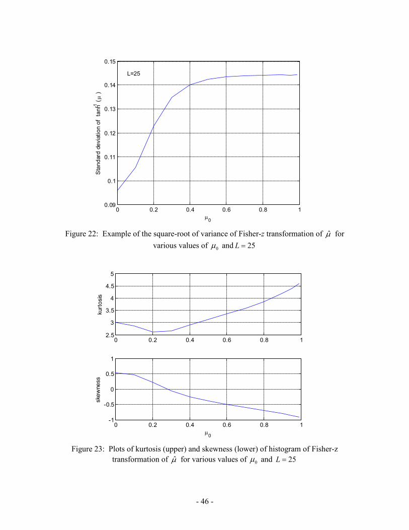
Figure 22: Example of the square-root of variance of Fisher-z transformation of µ̂ for

various values of 0µ and 25L =

Figure 23: Plots of kurtosis (upper) and skewness (lower) of histogram of Fisher-z

transformation of µ̂ for various values of 0µ and 25L =

0 0.2 0.4 0.6 0.8 10.09

0.1

0.11

0.12

0.13

0.14

0.15

Sta

ndar

d de

viat

ion

of t

anh-1

( µ

)

µ0

L=25

0 0.2 0.4 0.6 0.8 1-1

-0.5

0

0.5

1

skew

ness

µ0

0 0.2 0.4 0.6 0.8 12.5

3

3.5

4

4.5

5

kurt

osis

- 46 -

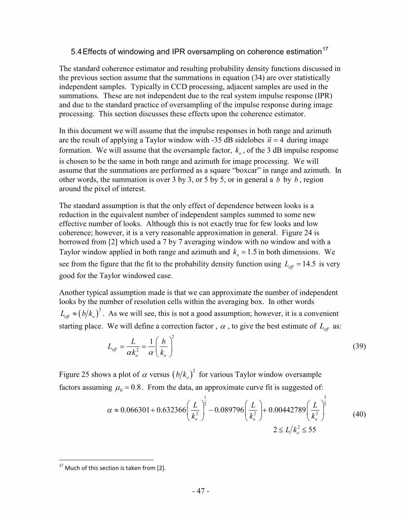
5.4 Effects of windowing and IPR oversampling on coherence estimation17

The standard coherence estimator and resulting probability density functions discussed in the previous section assume that the summations in equation (34) are over statistically independent samples. Typically in CCD processing, adjacent samples are used in the summations. These are not independent due to the real system impulse response (IPR) and due to the standard practice of oversampling of the impulse response during image processing. This section discusses these effects upon the coherence estimator.

In this document we will assume that the impulse responses in both range and azimuth are the result of applying a Taylor window with -35 dB sidelobes 4n = during image formation. We will assume that the oversample factor, ok , of the 3 dB impulse response is chosen to be the same in both range and azimuth for image processing. We will assume that the summations are performed as a square “boxcar” in range and azimuth. In other words, the summation is over 3 by 3, or 5 by 5, or in general a b by b , region around the pixel of interest.

The standard assumption is that the only effect of dependence between looks is a reduction in the equivalent number of independent samples summed to some new effective number of looks. Although this is not exactly true for few looks and low coherence; however, it is a very reasonable approximation in general. Figure 24 is borrowed from [2] which used a 7 by 7 averaging window with no window and with a Taylor window applied in both range and azimuth and 1.5ok = in both dimensions. We see from the figure that the fit to the probability density function using 14.5effL = is very good for the Taylor windowed case.

Another typical assumption made is that we can approximate the number of independent looks by the number of resolution cells within the averaging box. In other words

( )2eff oL b k≈ . As we will see, this is not a good assumption; however, it is a convenient

starting place. We will define a correction factor , α , to give the best estimate of effL as: 2

21

effo o

L bLk kα α

= =

(39)

Figure 25 shows a plot of α versus ( )2ob k for various Taylor window oversample

factors assuming 0 0.8µ = . From the data, an approximate curve fit is suggested of: 1 32 2

2 2 2

2

0.066301 0.632366 0.089796 0.00442789

2 55o o o

o

L L Lk k k

L k

α

≈ + − +

≤ ≤

(40)

17 Much of this section is taken from [2].

- 47 -

Figure 24: Example of effective number of looks on pdf of µ̂ using 7 by 7 averaging

for the coherence estimator

Figure 25: Plot of α versus 2

oL k for differing values of ok

0 0.2 0.4 0.6 0.8 10

2

4

6

8

10

12

pdf

µ

Simulated independentSimulated Taylor ko=1.5

Exact pdf L=49Exact pdf Leff = 14.5

0 10 20 30 40 50 600.7

0.8

0.9

1

1.1

1.2

1.3

1.4

1.5

1.6

1.7

L / ko2

α

ko=1.2

ko=1.5

ko=2.0

fit

- 48 -

Note that this curve fit will have issues for lower values of ( )2ob k and ok .

The implication of the discussion above is that the use of a window function and oversampling reduces the effective number of independent samples used in the estimator of the coherence. From a previous section, we know that the bias and variance of the coherence estimator increases with decreasing number of independent samples averaged.

- 49 -

6. Conclusions This report has attempted to bring together information about coherence and coherence estimation from various sources into a single document. The application of this document is intended to support the understanding of coherent change detection (CCD) for radar system designers.

- 50 -

7. References [1] D. L. Bickel, W. H. Hensley, “Design, Theory, and Applications of lnterferometric Synthetic Aperture Radar for Topographic Mapping”, SAND96-1092, May, 1996.

[2] D. L. Bickel, various internal memorandums dated 1999-2012.

[3] D. Just, R. Bamler, “Phase statistics of interferograms with applications to synthetic aperture radar” Applied Optics, Vol. 33, Iss. 20, July 10, 1994.

[4] C. V. Jakowatz, Jr., D. E. Wahl, P. H. Eichel, D. C. Ghiglia, P. A. Thompson, Spotlight-Mode Synthetic Aperture Radar: A Signal Processing Approach, Kluwer Academic Publishers, 1996.

[5] R. A. Fisher, “On the ‘Probable Error’ of a Coefficient of Correlation Deduced from a Small Sample,” Metron, vol. 1, no. 5, pp. 3-32, 1921.

[6] J. W. Goodman, Statistical Optics, John Wiley & Sons, Inc., 1985.

[7] A. W. Doerry, “Anatomy of a SAR Impulse Response”, SAND2007-5042, August 2007.

[8] A. W. Doerry, private notes on interpolation, June 19, 2011.

[9] R. Hanssen and R. Bamler, “Evaluation of interpolation kernels for SAR interferometry,” IEEE Transactions on Geoscience and Remote Sensing, vol. 37, no. 1, pp. 318-321, Jan. 1999.

[10] H. Skrivner, J. Dall, S. Madsen, “External polarimetric calibration of the Danish polarimetric C-band SAR”, Proceedings of IGARSS '94, Vol. 2, pp. 1105-1107, Aug, 1994.

[11] D. Barton, Modern Radar System Analysis, Artech House, 1988.

[12] H. A. Zebker, J. Villasenor, “Decorrelation in interferometric radar echoes”, IEEE Trans. On Geoscience and Remote Sensing, Vol. 30, Iss. 5, 1992.

[13] J. Villasenor, H. Zebker, “Temporal Decorrelation in Repeat-Pass Radar Interferometry”, Proceedings of IGARSS’92, Vol. 2, pp. 941-943, 1992.

[14] R. Touzi, A. Lopes, J. Bruniquel, P. W. Vachon, “Coherence estimation for SAR imagery”, IEEE Transactions on Geoscience and Remote Sensing, Vol. 27, Iss. 1, January, 1999.

- 51 -

8. Appendix A: Symbols and terminology Variable definitions

B - the bandwidth of the SAR image b - number of pixels on a side of a “boxcar” averaging δ - registration error

ok - IPR oversample, i.e., reciprocal of the number of resolution cells within a pixel (note that this is NOT the Nyquist oversample factor)

rf - frequency of relative ramp between the SAR images sf - the sampling frequency ( )H f - the transfer function of the SAR image

( )I f - the transfer function of the interpolation IPR - impulse response mnr - multiplicative noise ratio

0µ - the expected value of the coherence (often used to mean the magnitude of this quantity)

µ̂ - the estimate of the coherence (often used to mean the magnitude of this quantity)

µ - used as a general variable for coherence (or in figure labels used for µ̂ )

cubicµ - coherence component due to a residual cubic phase error

geomµ - coherence component due to collection geometry differences

,geom atrkµ - coherence component due to collection geometry differences in along track

,geom xtrkµ - coherence component due to collection geometry differences in cross-track

interpµ - coherence component due to interpolation

iprµ - coherence component due to impulse response mismatch

polµ - coherence component due to changes in polarization between passes

randµ - coherence component due to random phase errors

regµ - coherence component due to registration errors

rwµ - coherence component due to range-walk correction differences between images

sinusoidµ - coherence component due to sinusoidal phase error in one of the images

snrµ - coherence component due to thermal noise

quadµ - coherence component due to a residual quadratic phase error

- 52 -

L - number of “looks” averaged to estimate the coherence effL - apparent number of independent “looks” in an averaging process for

coherence estimation λ - radar wavelength

offsetθ∆ - difference in azimuth angles between SAR images ρ - resolution of the SAR images

aρ - azimuth resolution of the SAR images

rρ - slant range resolution of the SAR images η - is the terrain slope angle, positive when sloping towards the radar snr - signal-to-noise ratio, assumed equal between images (unitless)

isnr - signal-to-noise ratio of ith image (unitless)

φσ - standard deviation of random phase noise

,i nx - the nth pixel within the ith image ψ - grazing angle of SAR image ψ∆ - difference in grazing angles between the SAR images

z - Fisher z-transform of coherence estimate variable z - Fisher z-transform of coherence estimate variable

- 53 -

9. Distribution Unlimited Release

1 MS 0509 K. D. Meeks 5300 1 MS 0532 J. J. Hudgens 5340 1 MS 0532 B. L. Burns 5340 1 MS 0533 S. Gardner 5342 (electronic copy) 1 MS 0533 T. P. Bielek 5342 (electronic copy) 1 MS 0533 D. Harmony 5342 (electronic copy) 1 MS 0533 J. A. Hollowell 5342 (electronic copy) 1 MS 0533 R. Riley 5342 (electronic copy) 1 MS 0533 B. G. Rush 5342 (electronic copy) 1 MS 0533 D. G. Thompson 5342 (electronic copy) 1 MS 0501 N. Padilla 5343 (electronic copy) 1 MS 0532 W. H. Hensley 5344 1 MS 0532 E. D. Gentry 5344 (electronic copy) 1 MS 0532 C. Musgrove 5344 (electronic copy) 1 MS 0519 R. M. Naething 5344 (electronic copy) 1 MS 0519 A. M. Raynal 5344 (electronic copy) 1 MS 0533 K. W. Sorensen 5345 (electronic copy) 1 MS 0533 B. C. Brock 5345 (electronic copy) 1 MS 0533 D. F. Dubbert 5345 (electronic copy) 1 MS 0519 S. P. Castillo 5346 (electronic copy) 1 MS 0519 R. D. West 5346 (electronic copy) 1 MS 0532 T. J. Trodden 5348 (electronic copy) 1 MS 0533 D. M. Small 5348 (electronic copy) 1 MS 0519 J. A. Ruffner 5349 1 MS 0519 L. M. Klein 5349 1 MS 0519 J. G. Chow 5349 (electronic copy) 1 MS 0519 A. W. Doerry 5349 6 MS 0519 D. L. Bickel 5354 1 MS 0519 R. C. Ormesher 5354 (electronic copy) 1 MS 0899 Technical Library 9536 (electronic copy)

- 54 -