
SAP HANA Business Function Library (BFL) · PUBLIC SAP HANA Platform 2.0 SPS 00 Document Version:...
158
PUBLIC SAP HANA Platform 2.0 SPS 00 Document Version: 1.0 – 2016-11-30 SAP HANA Business Function Library (BFL)
Transcript of SAP HANA Business Function Library (BFL) · PUBLIC SAP HANA Platform 2.0 SPS 00 Document Version:...

PUBLIC
SAP HANA Platform 2.0 SPS 00Document Version: 1.0 – 2016-11-30
SAP HANA Business Function Library (BFL)

Content
1 What is BFL?. . . . . . . . . . . . . . . . . . . . . . . . . . . . . . . . . . . . . . . . . . . . . . . . . . . . . . . . . . . . . . . 4
2 Getting Started with BFL. . . . . . . . . . . . . . . . . . . . . . . . . . . . . . . . . . . . . . . . . . . . . . . . . . . . . . 52.1 Prerequisites. . . . . . . . . . . . . . . . . . . . . . . . . . . . . . . . . . . . . . . . . . . . . . . . . . . . . . . . . . . . . . . . 52.2 Application Function Library (AFL). . . . . . . . . . . . . . . . . . . . . . . . . . . . . . . . . . . . . . . . . . . . . . . . .52.3 Security. . . . . . . . . . . . . . . . . . . . . . . . . . . . . . . . . . . . . . . . . . . . . . . . . . . . . . . . . . . . . . . . . . . .62.4 Checking BFL Installation. . . . . . . . . . . . . . . . . . . . . . . . . . . . . . . . . . . . . . . . . . . . . . . . . . . . . . . 72.5 Calling BFL Functions. . . . . . . . . . . . . . . . . . . . . . . . . . . . . . . . . . . . . . . . . . . . . . . . . . . . . . . . . . 7
Generating BFL Procedures. . . . . . . . . . . . . . . . . . . . . . . . . . . . . . . . . . . . . . . . . . . . . . . . . . . 72.6 Using BFL in SAP HANA AFM. . . . . . . . . . . . . . . . . . . . . . . . . . . . . . . . . . . . . . . . . . . . . . . . . . . . .9
3 BFL Functions. . . . . . . . . . . . . . . . . . . . . . . . . . . . . . . . . . . . . . . . . . . . . . . . . . . . . . . . . . . . . . 123.1 Annual Depreciation. . . . . . . . . . . . . . . . . . . . . . . . . . . . . . . . . . . . . . . . . . . . . . . . . . . . . . . . . . 15
Diminishing Balance Depreciation. . . . . . . . . . . . . . . . . . . . . . . . . . . . . . . . . . . . . . . . . . . . . . 15Straight-line Depreciation. . . . . . . . . . . . . . . . . . . . . . . . . . . . . . . . . . . . . . . . . . . . . . . . . . . . 17Sum-of-year Depreciation. . . . . . . . . . . . . . . . . . . . . . . . . . . . . . . . . . . . . . . . . . . . . . . . . . . .19
3.2 Cycles. . . . . . . . . . . . . . . . . . . . . . . . . . . . . . . . . . . . . . . . . . . . . . . . . . . . . . . . . . . . . . . . . . . . 203.3 Cumulate. . . . . . . . . . . . . . . . . . . . . . . . . . . . . . . . . . . . . . . . . . . . . . . . . . . . . . . . . . . . . . . . . .223.4 Days. . . . . . . . . . . . . . . . . . . . . . . . . . . . . . . . . . . . . . . . . . . . . . . . . . . . . . . . . . . . . . . . . . . . . 233.5 Days Outstanding. . . . . . . . . . . . . . . . . . . . . . . . . . . . . . . . . . . . . . . . . . . . . . . . . . . . . . . . . . . . 253.6 De-cumulate. . . . . . . . . . . . . . . . . . . . . . . . . . . . . . . . . . . . . . . . . . . . . . . . . . . . . . . . . . . . . . . 273.7 Delay. . . . . . . . . . . . . . . . . . . . . . . . . . . . . . . . . . . . . . . . . . . . . . . . . . . . . . . . . . . . . . . . . . . . .293.8 Delay Debt. . . . . . . . . . . . . . . . . . . . . . . . . . . . . . . . . . . . . . . . . . . . . . . . . . . . . . . . . . . . . . . . . 313.9 Delay Stock. . . . . . . . . . . . . . . . . . . . . . . . . . . . . . . . . . . . . . . . . . . . . . . . . . . . . . . . . . . . . . . . 343.10 Discounted Cash Flow. . . . . . . . . . . . . . . . . . . . . . . . . . . . . . . . . . . . . . . . . . . . . . . . . . . . . . . . .363.11 Driver. . . . . . . . . . . . . . . . . . . . . . . . . . . . . . . . . . . . . . . . . . . . . . . . . . . . . . . . . . . . . . . . . . . . 383.12 Feed. . . . . . . . . . . . . . . . . . . . . . . . . . . . . . . . . . . . . . . . . . . . . . . . . . . . . . . . . . . . . . . . . . . . . 413.13 Feed Overflow. . . . . . . . . . . . . . . . . . . . . . . . . . . . . . . . . . . . . . . . . . . . . . . . . . . . . . . . . . . . . . 423.14 Forecast. . . . . . . . . . . . . . . . . . . . . . . . . . . . . . . . . . . . . . . . . . . . . . . . . . . . . . . . . . . . . . . . . . 453.15 Forecast Agents. . . . . . . . . . . . . . . . . . . . . . . . . . . . . . . . . . . . . . . . . . . . . . . . . . . . . . . . . . . . . 483.16 Forecast Driver. . . . . . . . . . . . . . . . . . . . . . . . . . . . . . . . . . . . . . . . . . . . . . . . . . . . . . . . . . . . . 503.17 Forecast Dual Driver. . . . . . . . . . . . . . . . . . . . . . . . . . . . . . . . . . . . . . . . . . . . . . . . . . . . . . . . . . 533.18 Forecast Mix. . . . . . . . . . . . . . . . . . . . . . . . . . . . . . . . . . . . . . . . . . . . . . . . . . . . . . . . . . . . . . . 563.19 Forecast Sensitivity. . . . . . . . . . . . . . . . . . . . . . . . . . . . . . . . . . . . . . . . . . . . . . . . . . . . . . . . . . 583.20 Funds. . . . . . . . . . . . . . . . . . . . . . . . . . . . . . . . . . . . . . . . . . . . . . . . . . . . . . . . . . . . . . . . . . . . 623.21 Future. . . . . . . . . . . . . . . . . . . . . . . . . . . . . . . . . . . . . . . . . . . . . . . . . . . . . . . . . . . . . . . . . . . . 633.22 Grow. . . . . . . . . . . . . . . . . . . . . . . . . . . . . . . . . . . . . . . . . . . . . . . . . . . . . . . . . . . . . . . . . . . . . 66
2 P U B L I CSAP HANA Business Function Library (BFL)
Content

3.23 Inflated Cash Flow. . . . . . . . . . . . . . . . . . . . . . . . . . . . . . . . . . . . . . . . . . . . . . . . . . . . . . . . . . . 68
3.24 Internal Rate of Return (IRR). . . . . . . . . . . . . . . . . . . . . . . . . . . . . . . . . . . . . . . . . . . . . . . . . . . . 70
3.25 Lag. . . . . . . . . . . . . . . . . . . . . . . . . . . . . . . . . . . . . . . . . . . . . . . . . . . . . . . . . . . . . . . . . . . . . . 72
3.26 Last. . . . . . . . . . . . . . . . . . . . . . . . . . . . . . . . . . . . . . . . . . . . . . . . . . . . . . . . . . . . . . . . . . . . . .74
3.27 Lease. . . . . . . . . . . . . . . . . . . . . . . . . . . . . . . . . . . . . . . . . . . . . . . . . . . . . . . . . . . . . . . . . . . . 75
3.28 Lease Variable. . . . . . . . . . . . . . . . . . . . . . . . . . . . . . . . . . . . . . . . . . . . . . . . . . . . . . . . . . . . . . 79
3.29 Linear Average. . . . . . . . . . . . . . . . . . . . . . . . . . . . . . . . . . . . . . . . . . . . . . . . . . . . . . . . . . . . . . 83
3.30 Max Value. . . . . . . . . . . . . . . . . . . . . . . . . . . . . . . . . . . . . . . . . . . . . . . . . . . . . . . . . . . . . . . . . 85
3.31 Minimum Value. . . . . . . . . . . . . . . . . . . . . . . . . . . . . . . . . . . . . . . . . . . . . . . . . . . . . . . . . . . . . 86
3.32 Moving Average&Moving Sum. . . . . . . . . . . . . . . . . . . . . . . . . . . . . . . . . . . . . . . . . . . . . . . . . . . 87
3.33 Moving Median. . . . . . . . . . . . . . . . . . . . . . . . . . . . . . . . . . . . . . . . . . . . . . . . . . . . . . . . . . . . . .92
3.34 Number of Periods. . . . . . . . . . . . . . . . . . . . . . . . . . . . . . . . . . . . . . . . . . . . . . . . . . . . . . . . . . . 94
3.35 Net Present Value. . . . . . . . . . . . . . . . . . . . . . . . . . . . . . . . . . . . . . . . . . . . . . . . . . . . . . . . . . . .97
3.36 Outlook. . . . . . . . . . . . . . . . . . . . . . . . . . . . . . . . . . . . . . . . . . . . . . . . . . . . . . . . . . . . . . . . . . . 99
3.37 Payment. . . . . . . . . . . . . . . . . . . . . . . . . . . . . . . . . . . . . . . . . . . . . . . . . . . . . . . . . . . . . . . . . .101
3.38 Present Value. . . . . . . . . . . . . . . . . . . . . . . . . . . . . . . . . . . . . . . . . . . . . . . . . . . . . . . . . . . . . . 104
3.39 Proportion. . . . . . . . . . . . . . . . . . . . . . . . . . . . . . . . . . . . . . . . . . . . . . . . . . . . . . . . . . . . . . . . 106
3.40 Rate. . . . . . . . . . . . . . . . . . . . . . . . . . . . . . . . . . . . . . . . . . . . . . . . . . . . . . . . . . . . . . . . . . . . .108
3.41 Repeat. . . . . . . . . . . . . . . . . . . . . . . . . . . . . . . . . . . . . . . . . . . . . . . . . . . . . . . . . . . . . . . . . . . 110
3.42 Rounding. . . . . . . . . . . . . . . . . . . . . . . . . . . . . . . . . . . . . . . . . . . . . . . . . . . . . . . . . . . . . . . . . 112
3.43 Seasonal Simple&Seasonal Complex. . . . . . . . . . . . . . . . . . . . . . . . . . . . . . . . . . . . . . . . . . . . . .114
Seasonal Complex. . . . . . . . . . . . . . . . . . . . . . . . . . . . . . . . . . . . . . . . . . . . . . . . . . . . . . . . 116
Seasonal Simple. . . . . . . . . . . . . . . . . . . . . . . . . . . . . . . . . . . . . . . . . . . . . . . . . . . . . . . . . . 118
3.44 Seasonal Simulation. . . . . . . . . . . . . . . . . . . . . . . . . . . . . . . . . . . . . . . . . . . . . . . . . . . . . . . . . 121
3.45 Stock Flow. . . . . . . . . . . . . . . . . . . . . . . . . . . . . . . . . . . . . . . . . . . . . . . . . . . . . . . . . . . . . . . . 123
3.46 Stock Flow Reverse. . . . . . . . . . . . . . . . . . . . . . . . . . . . . . . . . . . . . . . . . . . . . . . . . . . . . . . . . . 130
3.47 Stock Flow Batch. . . . . . . . . . . . . . . . . . . . . . . . . . . . . . . . . . . . . . . . . . . . . . . . . . . . . . . . . . . 137
3.48 Time. . . . . . . . . . . . . . . . . . . . . . . . . . . . . . . . . . . . . . . . . . . . . . . . . . . . . . . . . . . . . . . . . . . . 144
3.49 Time Sum. . . . . . . . . . . . . . . . . . . . . . . . . . . . . . . . . . . . . . . . . . . . . . . . . . . . . . . . . . . . . . . . .146
3.50 Transform. . . . . . . . . . . . . . . . . . . . . . . . . . . . . . . . . . . . . . . . . . . . . . . . . . . . . . . . . . . . . . . . 149
3.51 Volume Driver. . . . . . . . . . . . . . . . . . . . . . . . . . . . . . . . . . . . . . . . . . . . . . . . . . . . . . . . . . . . . . 151
3.52 Year-Over-Year Difference. . . . . . . . . . . . . . . . . . . . . . . . . . . . . . . . . . . . . . . . . . . . . . . . . . . . . 152
3.53 Year to Date. . . . . . . . . . . . . . . . . . . . . . . . . . . . . . . . . . . . . . . . . . . . . . . . . . . . . . . . . . . . . . . 154
3.54 Year-to-Date Statistical. . . . . . . . . . . . . . . . . . . . . . . . . . . . . . . . . . . . . . . . . . . . . . . . . . . . . . . 155
SAP HANA Business Function Library (BFL)Content P U B L I C 3

1 What is BFL?
SAP HANA In-Memory Computing Engine offers various algorithms for in-memory computing. It provides several application libraries for developers, partners, and customers who develop applications that run on SAP HANA. The libraries are linked dynamically to the SAP HANA database kernel.
The Business Function Library (BFL) is one of these application libraries. It contains pre-built parameter-driven functions in the financial area. The functions are implemented by C++. This library helps you develop compound business algorithms that are fully compliant with the SAP HANA calculation engine. It offers you the flexibility and efficiency to develop HANA-based applications with incredible performance.
The BFL extends the computation ability of SAP HANA with complex and performance-critical algorithms which are requested by applications. By using the library, you can achieve:
● Significant performance improvement for SAP applications○ Utilizing new hardware (e.g. multi core, built-in vector engine)○ Massive parallel main memory processing○ Changing the boundaries between application server and data management layer
● Simplification of application programming model○ Usage of extended SQL (SQL script)○ Rich functionalities in calculation engine○ Quick application delivery
4 P U B L I CSAP HANA Business Function Library (BFL)
What is BFL?

2 Getting Started with BFL
This section covers the information you need to know to start working with the SAP HANA Business Function Library.
2.1 Prerequisites
To use the BFL functions, you must:
● Install SAP HANA Platform 2.0 SPS 00.● Install the Application Function Library (AFL), which includes the BFL.
For information on how to install or update AFL, see "Installing or Updating SAP HANA Components" in SAP HANA Server Installation and Update Guide:
NoteThe revision number of the AFL must match the revision number of SAP HANA. See SAP Note 1898497 for details.
● Enable the Script Server in HANA instance. See SAP Note 1650957 for further information.
Related Information
SAP HANA Server Installation and Update GuideSAP Note 1898497SAP Note 1650957
2.2 Application Function Library (AFL)
You can dramatically increase performance by executing complex computations in the database instead of at the application sever level. SAP HANA provides several techniques to move application logic into the database, and one of the most important is the use of application functions. Application functions are like database procedures written in C++ and called from outside to perform data intensive and complex operations.
Functions for a particular topic are grouped into an application function library (AFL), such as the Predictive Analysis Library (PAL) and the Business Function Library (BFL). Currently, PAL and BFL are delivered in one
SAP HANA Business Function Library (BFL)Getting Started with BFL P U B L I C 5

archive (that is, one SAR file with the name AFL<version_string>.SAR). The AFL archive is not part of the HANA appliance, and must be installed separately by the administrator.
2.3 Security
This section provides detailed security information which can help administrator and architects answer some common questions.
Role Assignment
For each AFL area, there are two roles. You must be assigned one of the roles to execute the functions in the library. The roles for the BFL library are automatically created when the Application Function Library (AFL) is installed. The role names are:
AFL__SYS_AFL_AFLBFL_EXECUTE
AFL__SYS_AFL_AFLBFL_EXECUTE_WITH_GRANT_OPTION
NoteThere are 2 underscores between AFL and SYS.
To generate or drop procedures for the following BFL functions, you also need the AFLPM_CREATOR_ERASER_EXECUTE role, which is created when SAP HANA is installed:
● Delay● Driver● Forecast Driver● Forecast Dual Driver● Moving Average & Moving Sum● Time Sum
NoteOnce the above roles are automatically created, they cannot be dropped. In other words, even when an area with all its objects is dropped and re-created during system startup, the user still keeps these roles originally granted.
6 P U B L I CSAP HANA Business Function Library (BFL)
Getting Started with BFL

2.4 Checking BFL Installation
To confirm that the BFL functions were installed successfully, you can check the following three public views:
● sys.afl_areas● sys.afl_packages● sys.afl_functions
These views are granted to the PUBLIC role and can be accessed by anyone.
To check the views, run the following SQL statements:
SELECT * FROM "SYS"."AFL_AREAS" WHERE AREA_NAME = 'AFLBFL'; SELECT * FROM "SYS"."AFL_PACKAGES" WHERE AREA_NAME = 'AFLBFL';SELECT * FROM "SYS"."AFL_FUNCTIONS" WHERE AREA_NAME = 'AFLBFL';
The result will tell you whether the BFL functions were successfully installed on your system.
2.5 Calling BFL Functions
Most of the functions can be called directly once the BFL library has been installed and the script server has started. The calling syntax is as follows:
CALL <schema_name>.AFLBFL_<function_name>_PROC(
{inputTab1,…}, <output_tab>) with overview;
● <schema_name>: The schema under which BFL functions are created.● AFLBFL: The name of the BFL library.● AFLBFL_<function_name>_PROC: The procedure name automatically generated by AFL.● {inputTab1,…}: User-defined name(s) of the current procedure’s input table(s). Detailed input table
definition for each procedure can be found in Chapter 3.● <output_tab>: User-defined name(s) of the current procedure’s output table(s). Detailed output table
definition for each procedure can be found in Chapter 3.
2.5.1 Generating BFL Procedures
The following functions require you to generate a procedure that wraps the function:
● Delay● Driver● Forecast Driver● Forecast Dual Driver
SAP HANA Business Function Library (BFL)Getting Started with BFL P U B L I C 7

● Moving Average & Moving Sum● Time Sum
Step 1 – Generate a BFL Procedure
Any user granted with the AFLPM_CREATOR_ERASER_EXECUTE role can generate an AFLLANG procedure for a specific BFL function. The syntax is shown below:
CALL SYS.AFLLANG_WRAPPER_PROCEDURE_CREATE (‘<area_name>’, ‘<function_name>’, ‘<schema_name>’, '<procedure_name>', <signature_table>);
● <area_name>: Always set to AFLBFL.● <function_name>: A BFL built-in function name.● <schema_name>: A name of the schema that you want to create.● <procedure_name>: A name for the BFL procedure. This can be anything you want.● <signature_table>: A user-defined table variable. The table contains records to describe the position,
schema name, table type name, and parameter type, as defined below:
( POSITION int,SCHEMA_NAME nvarchar(256),TYPE_NAME nvarchar(256),PARAMETER_TYPE varchar(7))
A typical table variable references a table with the following definition:
Table 1:
Position Schema Name Table Type Name Parameter Type
1 <schema_name> BFL_INPUT1_T IN
2 <schema_name> … IN
3 <schema_name> BFL_INPUTN_T IN
4 <schema_name> BFL_OUTPUT_T OUT
Note1. The records in the signature table must follow this order: first input table types, then the output table
types.2. The signature table must be created before generating the BFL procedure. The table type names are
user-defined. You can find detailed table type definitions for each BFL function in Chapter 3.3. If you want to drop an existing procedure and then generate it again, you need to call the
SYS.AFLLANG_WRAPPER_PROCEDURE_DROP procedure to clear the existing procedure. The syntax is as follows:
CALL SYS.AFLLANG_WRAPPER_PROCEDURE_DROP('<schema_name>','<procedure_name>');
4. The AFLLANG procedure generator described in this Step was introduced since SAP HANA Platform 1.0 SPS 09. For backward compatibility information, see SAP Note 2046767.
8 P U B L I CSAP HANA Business Function Library (BFL)
Getting Started with BFL

Step 2 – Call a BFL Procedure
After generating a BFL procedure, any user that has the AFL__SYS_AFL_AFLBFL_EXECUTE or AFL__SYS_AFL_AFLBFL_EXECUTE_WITH_GRANT_OPTION role can call the procedure by using the syntax below:
CALL <schema_name>.<procedure_name>( {input_table1,…}, <output_table>) with overview;
● <schema_name>: The name of the schema where the procedure is located.● <procedure_name>: The procedure name specified when generating the procedure in Step 1.● <input_table1,…>: User-defined name(s) of the procedure’s input table(s). Detailed input table
definitions for each procedure can be found in Chapter 3.● <output_table>: User-defined name of the procedure’s output table. Detailed output table definition for
each procedure can be found in Chapter 3.
Note1. The above tables must be created before calling the procedure.2. Some BFL algorithms have more than one input table.3. To call the BFL procedure generated in Step 1, you need the AFL__SYS_AFL_AFLBFL_EXECUTE or
AFL__SYS_AFL_AFLBFL_EXECUTE_WITH_GRANT_OPTION role.
Related Information
SAP Note 2046767
2.6 Using BFL in SAP HANA AFM
The SAP HANA Application Function Modeler (AFM) in SAP HANA Studio supports functions from BFL in flowgraph models. With the AFM, you can easily add BFL function nodes to your flowgraph, specify its parameters and input/output table types, and generate the procedure, all without writing any SQLScript code. You can also execute the procedure to get the output result of the function, and save the auto-generated SQLScript code for future use.
The main procedure is as follows:
1. Create a new flowgraph or open an existing flowgraph in the Project Explorer view.
NoteFor details on how to create a flowgraph, see "Creating a Flowgraph" in SAP HANA Developer Guide for SAP HANA Studio
SAP HANA Business Function Library (BFL)Getting Started with BFL P U B L I C 9

2. Specify the target schema by selecting the flowgraph container and editing Target Schema in the Properties view.
3. Add the input(s) for the flowgraph by doing the following:1. Right-click the input anchor region on the left side of the flowgraph container and choose Add Input.2. Edit the table types of the input by editing the signature the Properties view.
NoteYou can also drag a table from the catalog in the Systems view to the input anchor region of the flowgraph container.
4. Add a BFL function to the flowgraph by doing the following:1. Drag the function node from the Business Function Library compartment of the Palette to the
flowgraph editing area.2. Specify the input table types of the function by selecting the input anchor and editing its signature in
the Properties view.3. Specify the parameters of the function by selecting the parameter input anchor and editing its
signature and fixed content in the Properties view.
NoteA parameter table usually has fixed table content. If you want to supply the parameter values later when you execute the procedure, clear the Fixed Content option.
4. Specify the output table types of the function by selecting the output anchor and editing the signature in the Properties view.
5. (Optional) You can add more BFL nodes to the flowgraph if needed and connect them by holding the
Connect button from the source anchor and dragging a connection to the destination anchor.6. Connect the input(s) in the input anchor region of the flowgraph container to the required input anchor(s)
of the BFL function node.7. For the output tables that you want to see the output result after procedure execution, add them to the
output anchor region on the right side of the flowgraph container. To do that, move your mouse cursor
over the output anchor of the function node, hold the Connect button , and drag a connection to the output anchor region.
8. Save the flowgraph by choosing File Save in the HANA Studio main menu.
9. Activate the flowgraph by right-clicking the flowgraph in the Project Explorer view and choosing TeamActivate .A new procedure is generated in the target schema which is specified in Step 2.
NoteTo activate the flowgraph, the database user _SYS_REPO needs SELECT object privileges for objects that are used as data sources.
10. Select the black downward triangle next to the Execute button in the top right corner of the AFM.A context menu appears. It shows the options Execute in SQL Editor and Open in SQL Editor as well as the option Execute and Explore for every output of the flowgraph. In addition, the context menu shows the option Edit Input Bindings.
10 P U B L I CSAP HANA Business Function Library (BFL)
Getting Started with BFL

11. (Optional) If the flowgraph has input tables without fixed content, choose the option Edit Input Bindings.A wizard appears that allows you to bind all inputs of the flowgraph to data sources in the catalog.
NoteIf you do not bind the inputs, AFM will automatically open this wizard when executing the procedure.
12. Choose one of the options Execute in SQL Editor, Open in SQL Editor, or Execute and Explore for one of the outputs of the flowgraph.The behavior of the AFM depends on the execution mode.○ Open in SQL Editor: Opens a SQL console containing the SQL code to execute the runtime object.○ Execute in SQL Editor: Opens a SQL console containing the SQL code to execute the runtime object
and runs this SQL code.○ Execute and Explore: Executes the runtime object and opens the Data Explorer view for the chosen
output of the flowgraph.
13. Close the flowgraph by choosing File Close in the HANA Studio main menu.
For more information on how to use AFM, see the "Transforming Data Using SAP HANA Application Function Modeler"section in SAP HANA Developer Guide for SAP HANA Studio.
Related Information
SAP HANA Developer Guide for SAP HANA Studio
SAP HANA Business Function Library (BFL)Getting Started with BFL P U B L I C 11

3 BFL Functions
The following lists all available functions in the Business Function Library.
Table 2:
Function Description
Annual Depreciation [page 15] Calculates annual depreciation according to three common methods: Diminishing Balance Depreciation [page 15], Straight-line Depreciation [page 17], and Sum-of-year Depreciation [page 19]. It allows variable length of timescales for all assets/items.
Cycles [page 20] Calculates seasonal factors from Fourier coefficients. It combines sine and cosine waves to help you determine seasonality or other cyclical business factors.
Cumulate [page 22] Calculates the cumulative totals in one row based on the original numbers in another row.
Days [page 23] Returns the number of days in each period defined by each pair of From and To dates.
Days Outstanding [page 25] Calculates receipts or payments based on the level of days outstanding.
De-cumulate [page 27] Calculates the original series starting from the cumulated totals.
Delay [page 29] Calculates receivables or payables based on a delay between the time of invoice and the time of payment.
Delay Debt [page 31] Calculates cash receipts using actual sales. The closing debtor balance for each period is calculated by referring to historic sales levels for a specified number of days.
Delay Stock [page 34] Calculates purchases required to meet future demand.
Discounted Cash Flow [page 36] Converts a future stream of cash flow to constant prices. It calculates the inflated value of today's money.
Driver [page 38] Calculates the forecast for future periods using historical data and as many drivers as needed. A driver drives cost, such as headcount, floor space, units sold, and unit price.
Feed [page 41] Calculates the closing balance and "feeds" it to the opening balance of the next time period.
Feed Overflow [page 42] Calculates the closing balance and feeds it to the opening balance of the next time period.
Forecast [page 45] Combines actual and forecast data to produce a rolling forecast. Eliminates scripting of feeds.
12 P U B L I CSAP HANA Business Function Library (BFL)
BFL Functions

Function Description
Forecast Agents [page 48] A specialized version of the Driver function focused on the entities required to meet service levels. Used primarily for labor in areas like call centers and mortgage processing based on interest rate.
Forecast Driver [page 50] A specialized version of the Driver function that calculates the forecast for future periods using historical data and one single driver.
Forecast Dual Driver [page 53] Calculates the forecast for future periods using historical data and two drivers. It also calculates the incremental effect of each driver on the historical base figure.
Forecast Mix [page 56] Mixes actual data prior to the switchover date with forecast data on and after the switchover date.
Forecast Sensitivity [page 58] Returns a calculation for the proportion of requests that will be queued because there were no agents available when the request was answered.
Funds [page 62] Calculates the use of funds or the source of funds.
Future [page 63] Calculates the closing balance of an account given the start balance and the conditions under which the account runs.
Grow [page 66] Grows a base figure by a specified percentage each period. It can be compound or linear.
Inflated Cash Flow [page 68] Calculates the amount of cash you must receive in a future period to compensate for inflation.
Internal Rate of Return (IRR) [page 70] Calculates the internal rate of return for a series of cash flow on specified dates.
Lag [page 72] Calculates a result in one row by lagging an input from another row by a specified number of periods.
Last [page 74] Looks back over the series of data of the input row and returns the most recent non-zero value.
Lease [page 75] Calculates a payment schedule for a lease, loan, mortgage, annuity or savings account.
Lease Variable [page 79] Allows an account to be scheduled along a time scale representing the life of the loan.
Linear Average [page 83] Calculates a linear average that applies a larger weight to more recent periods. The weights applied decrease linearly as time goes backward.
Max Value [page 85] Returns the maximum value of a range.
Minimum Value [page 86] Returns the minimum value of a specific range.
Moving Average&Moving Sum [page 87] Calculates a moving average or moving sum over specified periods. Key statistical component
Moving Median [page 92] Takes the median value after sorting all input values into an ascending sequence.
Number of Periods [page 94] Calculates the number of periods over which the account must run.
SAP HANA Business Function Library (BFL)BFL Functions P U B L I C 13

Function Description
Net Present Value [page 97] Calculates the sum of a series of future cash flow values after discounting each to a present value based on the annual rate input for the period in which it is being calculated.
Outlook [page 99] The outlook is calculated by using actuals of past months and plan figures of future months.
Payment [page 101] Calculates the regular payment to an account for each period.
Present Value [page 104] Calculates opening value through the given target closing balance and various parameters.
Proportion [page 106] Allows you to input a start and end date, and then calculates the proportion of the period length. Important for project planning with performance to plan calculations
Rate [page 108] Calculates the percentage interest rate per period for an account, given its start balance, end balance, payment amount per period and the number of periods.
Repeat [page 110] It is used to repeat data from a single period or group of periods through the time scale of the Dimension List.
Rounding [page 112] Calculates the rounded values for a specified input item according to a chosen rounding method.
Seasonal Simple&Seasonal Complex [page 114] Performs seasonal adjustments of time to determine seasonal patterns in data.
Seasonal Simple [page 118] Performs seasonal adjustments of time to determine seasonal patterns in data.
Seasonal Simulation [page 121] Provides the building blocks to seasonal simulation seasonal data using a variety of characteristics.
Stock Flow [page 123] Works out the level of supply needed to meet target forecasts for stock cover.
Stock Flow Reverse [page 130] Allows you to input stock cover and work out what purchases were needed to meet the target stock levels.
Stock Flow Batch [page 137] Let’s you use batch quantities in stock flow calculations. Key for constraint based models or non-discrete manufacturing units of measure.
Time [page 144] Returns the information requested by the option you have input. Eliminates scripting of alternative time dimensions
Time Sum [page 146] Allows you to accumulate an expense over a specified number of periods in advance or arrears.
Transform [page 149] Helps users to build equations using angles and trigonometry functions when Cycles does not provide the functionality that they need.
Volume Driver [page 151] Calculates the year-over-year percentage difference for each volume driver.
Year-Over-Year Difference [page 152] Calculates the year over year difference between the current and previous time periods.
14 P U B L I CSAP HANA Business Function Library (BFL)
BFL Functions

Function Description
Year to Date [page 154] Calculates year to date totals based on original data.
Year-to-Date Statistical [page 155] Calculates the original numbers in one row based on the year-to-date figures in another row.
3.1 Annual Depreciation
This function calculates annual depreciation according to three common methods: Diminishing balance depreciation, Straight line depreciation and Sum-of-year depreciation. It allows variable length of timescales for all assets/items. This is critical for seasonality and creating adjusting periods.
3.1.1 Diminishing Balance Depreciation
This function calculates depreciation based on diminishing balances. It provides a higher depreciation charge in the first year of an asset’s life and gradually decreases charges in subsequent years. Depreciation is calculated by taking out the accumulated depreciation from the opening asset capitalization. Depreciation starts high, progressively decreases. The asset will never be fully depreciated.
Formula
Depreciation = (Capitalization - Accumulated depreciation to date) * (rate / 100)
Signature
Input Tables
Table 3:
Name Direction Number of Columns
Column Type Column Name Description
Capitalization Input Table 1 Double VALUE Asset capitalization (the cost of purchase)
Rate Input Table 1 Double VALUE The life of the capitalized asset in years
SAP HANA Business Function Library (BFL)BFL Functions P U B L I C 15
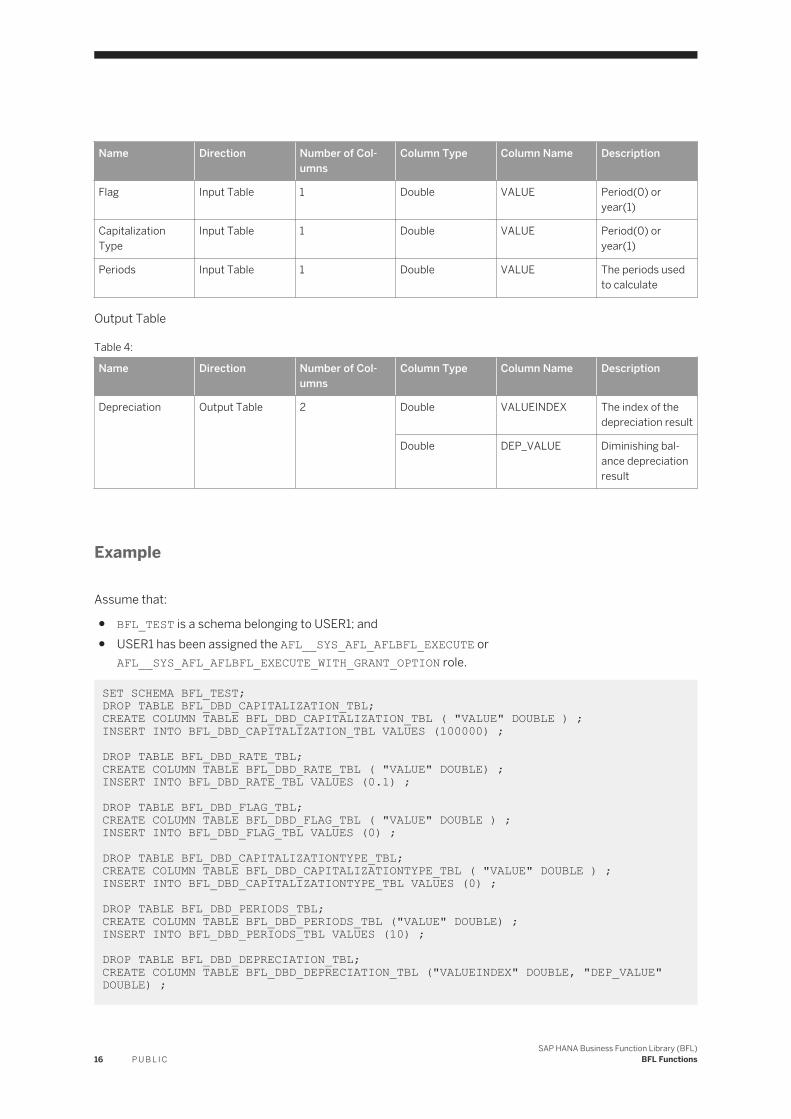
Name Direction Number of Columns
Column Type Column Name Description
Flag Input Table 1 Double VALUE Period(0) or year(1)
Capitalization Type
Input Table 1 Double VALUE Period(0) or year(1)
Periods Input Table 1 Double VALUE The periods used to calculate
Output Table
Table 4:
Name Direction Number of Columns
Column Type Column Name Description
Depreciation Output Table 2 Double VALUEINDEX The index of the depreciation result
Double DEP_VALUE Diminishing balance depreciation result
Example
Assume that:
● BFL_TEST is a schema belonging to USER1; and● USER1 has been assigned the AFL__SYS_AFL_AFLBFL_EXECUTE or
AFL__SYS_AFL_AFLBFL_EXECUTE_WITH_GRANT_OPTION role.
SET SCHEMA BFL_TEST;DROP TABLE BFL_DBD_CAPITALIZATION_TBL;CREATE COLUMN TABLE BFL_DBD_CAPITALIZATION_TBL ( "VALUE" DOUBLE ) ;INSERT INTO BFL_DBD_CAPITALIZATION_TBL VALUES (100000) ; DROP TABLE BFL_DBD_RATE_TBL;CREATE COLUMN TABLE BFL_DBD_RATE_TBL ( "VALUE" DOUBLE) ;INSERT INTO BFL_DBD_RATE_TBL VALUES (0.1) ; DROP TABLE BFL_DBD_FLAG_TBL;CREATE COLUMN TABLE BFL_DBD_FLAG_TBL ( "VALUE" DOUBLE ) ;INSERT INTO BFL_DBD_FLAG_TBL VALUES (0) ; DROP TABLE BFL_DBD_CAPITALIZATIONTYPE_TBL;CREATE COLUMN TABLE BFL_DBD_CAPITALIZATIONTYPE_TBL ( "VALUE" DOUBLE ) ;INSERT INTO BFL_DBD_CAPITALIZATIONTYPE_TBL VALUES (0) ; DROP TABLE BFL_DBD_PERIODS_TBL;CREATE COLUMN TABLE BFL_DBD_PERIODS_TBL ("VALUE" DOUBLE) ;INSERT INTO BFL_DBD_PERIODS_TBL VALUES (10) ; DROP TABLE BFL_DBD_DEPRECIATION_TBL;CREATE COLUMN TABLE BFL_DBD_DEPRECIATION_TBL ("VALUEINDEX" DOUBLE, "DEP_VALUE" DOUBLE) ;
16 P U B L I CSAP HANA Business Function Library (BFL)
BFL Functions

CALL _SYS_AFL.AFLBFL_DBDEPRECIATION_PROC (BFL_DBD_CAPITALIZATION_TBL, BFL_DBD_RATE_TBL, BFL_DBD_FLAG_TBL, BFL_DBD_CAPITALIZATIONTYPE_TBL, BFL_DBD_PERIODS_TBL, BFL_DBD_DEPRECIATION_TBL) WITH OVERVIEW; SELECT * FROM BFL_DBD_DEPRECIATION_TBL;
3.1.2 Straight-line Depreciation
This function can help companies to estimate the residual value of each asset which is used during the production process.
It calculates depreciation by dividing the asset capitalization by the life of it based on two inputs.
1. Asset capitalization2. The life in periods or years.
Formula
Depreciation = Capitalization / Life of the asset
Signature
Input Tables
Table 5:
Name Direction Number of Columns
Column Type Column Name Description
Capitalization Input Table 1 Double VALUE Asset capitalization (the cost of purchase)
Life Input Table 1 Double VALUE Life of the asset. Possible to import from NWBI or other ledger
Flag Input Table 1 Double VALUE Period(0) or year(1)
Output Table
SAP HANA Business Function Library (BFL)BFL Functions P U B L I C 17

Table 6:
Name Direction Number of Columns
Column Type Column Name Description
Depreciation Output Table 2 Double VALUEINDEX The index of the depreciation result
Double DEP_VALUE Straight line depreciation result
Example
Assume that:
● BFL_TEST is a schema belonging to USER1; and● USER1 has been assigned the AFL__SYS_AFL_AFLBFL_EXECUTE or
AFL__SYS_AFL_AFLBFL_EXECUTE_WITH_GRANT_OPTION role.
SET SCHEMA BFL_TEST; DROP TABLE BFL_SLD_CAPITALIZATION_TBL;CREATE COLUMN TABLE BFL_SLD_CAPITALIZATION_TBL ( "VALUE" DOUBLE ) ;INSERT INTO BFL_SLD_CAPITALIZATION_TBL VALUES (2400);INSERT INTO BFL_SLD_CAPITALIZATION_TBL VALUES (0);INSERT INTO BFL_SLD_CAPITALIZATION_TBL VALUES (0);INSERT INTO BFL_SLD_CAPITALIZATION_TBL VALUES (0);INSERT INTO BFL_SLD_CAPITALIZATION_TBL VALUES (0);INSERT INTO BFL_SLD_CAPITALIZATION_TBL VALUES (0);INSERT INTO BFL_SLD_CAPITALIZATION_TBL VALUES (0);INSERT INTO BFL_SLD_CAPITALIZATION_TBL VALUES (0);INSERT INTO BFL_SLD_CAPITALIZATION_TBL VALUES (0);INSERT INTO BFL_SLD_CAPITALIZATION_TBL VALUES (0);INSERT INTO BFL_SLD_CAPITALIZATION_TBL VALUES (0);INSERT INTO BFL_SLD_CAPITALIZATION_TBL VALUES (0); DROP TABLE BFL_SLD_LIFE_TBL ;CREATE COLUMN TABLE BFL_SLD_LIFE_TBL( "VALUE" DOUBLE );INSERT INTO BFL_SLD_LIFE_TBL VALUES (10); DROP TABLE BFL_SLD_FLAG_TBL ;CREATE COLUMN TABLE BFL_SLD_FLAG_TBL ( "VALUE" DOUBLE );INSERT INTO BFL_SLD_FLAG_TBL VALUES (1) ; DROP TABLE BFL_SLD_DEPRECIATION_TBL ;CREATE COLUMN TABLE BFL_SLD_DEPRECIATION_TBL ( "VALUEINDEX" DOUBLE, "DEP_VALUE" DOUBLE) ;result tables CALL _SYS_AFL.AFLBFL_SLDEPRECIATION_PROC (BFL_SLD_CAPITALIZATION_TBL, BFL_SLD_LIFE_TBL, BFL_SLD_FLAG_TBL, BFL_SLD_DEPRECIATION_TBL) with overview; SELECT * FROM BFL_SLD_DEPRECIATION_TBL ;
18 P U B L I CSAP HANA Business Function Library (BFL)
BFL Functions
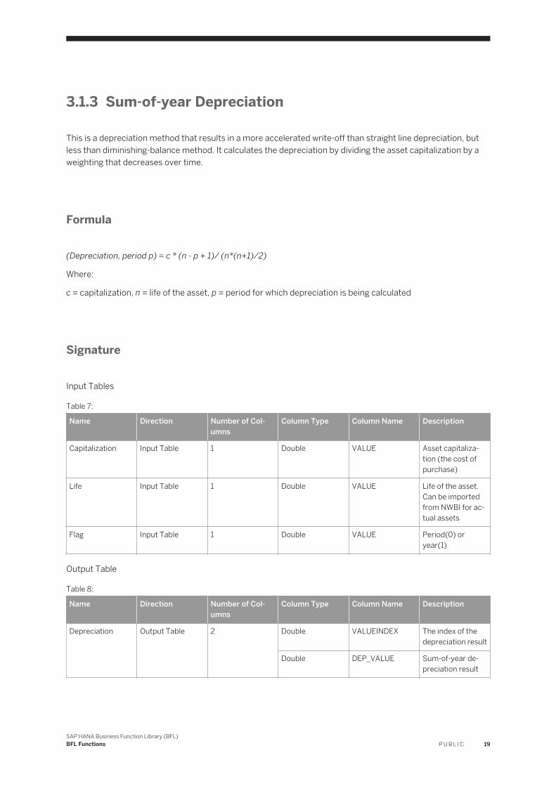
3.1.3 Sum-of-year Depreciation
This is a depreciation method that results in a more accelerated write-off than straight line depreciation, but less than diminishing-balance method. It calculates the depreciation by dividing the asset capitalization by a weighting that decreases over time.
Formula
(Depreciation, period p) = c * (n - p + 1)/ (n*(n+1)/2)
Where:
c = capitalization, n = life of the asset, p = period for which depreciation is being calculated
Signature
Input Tables
Table 7:
Name Direction Number of Columns
Column Type Column Name Description
Capitalization Input Table 1 Double VALUE Asset capitalization (the cost of purchase)
Life Input Table 1 Double VALUE Life of the asset. Can be imported from NWBI for actual assets
Flag Input Table 1 Double VALUE Period(0) or year(1)
Output Table
Table 8:
Name Direction Number of Columns
Column Type Column Name Description
Depreciation Output Table 2 Double VALUEINDEX The index of the depreciation result
Double DEP_VALUE Sum-of-year depreciation result
SAP HANA Business Function Library (BFL)BFL Functions P U B L I C 19

Example
Assume that:
● BFL_TEST is a schema belonging to USER1; and● USER1 has been assigned the AFL__SYS_AFL_AFLBFL_EXECUTE or
AFL__SYS_AFL_AFLBFL_EXECUTE_WITH_GRANT_OPTION role.
SET SCHEMA BFL_TEST; DROP TABLE BFL_SYD_CAPITALIZATION_TBL ;CREATE COLUMN TABLE BFL_SYD_CAPITALIZATION_TBL ( "VALUE" DOUBLE ) ;INSERT INTO BFL_SYD_CAPITALIZATION_TBL VALUES (15000); DROP TABLE BFL_SYD_LIFE_TBL ;CREATE COLUMN TABLE BFL_SYD_LIFE_TBL( "VALUE" DOUBLE );INSERT INTO BFL_SYD_LIFE_TBL VALUES (5);DROP TABLE BFL_SYD_FLAG_TBL ;CREATE COLUMN TABLE BFL_SYD_FLAG_TBL ( "VALUE" DOUBLE );INSERT INTO BFL_SYD_FLAG_TBL VALUES (0) ;DROP TABLE BFL_SYD_DEPRECIATION_TBL ;CREATE COLUMN TABLE BFL_SYD_DEPRECIATION_TBL ( "VALUEINDEX" DOUBLE, "DEP_VALUE" DOUBLE) ; CALL _SYS_AFL.AFLBFL_SOYDEPRECIATION_PROC (BFL_SYD_CAPITALIZATION_TBL, BFL_SYD_LIFE_TBL, BFL_SYD_FLAG_TBL, BFL_SYD_DEPRECIATION_TBL) with overview; SELECT * FROM BFL_SYD_DEPRECIATION_TBL ;
3.2 Cycles
Cycles calculates seasonal factors by using Fourier coefficients. It combines sine and cosine waves to help you determine seasonality or other cyclical business factors.
Formula
● When {sine/cosine} = sine, the equation is:
{Cycle} = {amplitude} * Sin(360 * ({time} - {start date}) / {length})
● When {sine/cosine}= cosine, the equation is:
{Cycle}= {amplitude} * Cos(360 * ( {time} - {start date}) / {length})
Where: {time} is the center of the period.
Signature
Input Tables
20 P U B L I CSAP HANA Business Function Library (BFL)
BFL Functions

Table 9:
Name Direction Number of Columns
Column Type Column Name Description
Amplitude Input Table 1 Double AMPLITUDE Amplitude of sine/cosine.
Length Input Table 1 Double LENGTH Length (in years) over which the cycle repeats itself.
Startdate Input Table 1 Double START Time in years at which the cycle starts.
Function Input Table 1 Int FUNCTION 0 for a sine wave, and 1 for a cosine wave.
Time Input Table 1 Double TIME Time periods.
Output Table
Table 10:
Name Direction Number of Columns
Column Type Column Name Description
Result Output Table 1 Double CYCLE Result table that contains the expected result.
Example
Assume that:
● BFL_TEST is a schema belonging to USER1; and● USER1 has been assigned the AFL__SYS_AFL_AFLBFL_EXECUTE or
AFL__SYS_AFL_AFLBFL_EXECUTE_WITH_GRANT_OPTION role.
SET SCHEMA BFL_TEST; DROP TABLE BFL_CYCLES_AMPLITUDE_TBL;CREATE COLUMN TABLE BFL_CYCLES_AMPLITUDE_TBL( "AMPLITUDE" DOUBLE ) ;INSERT INTO BFL_CYCLES_AMPLITUDE_TBL VALUES (200) ;INSERT INTO BFL_CYCLES_AMPLITUDE_TBL VALUES (300) ;INSERT INTO BFL_CYCLES_AMPLITUDE_TBL VALUES (2000) ;DROP TABLE BFL_CYCLES_LENGTH_TBL;CREATE COLUMN TABLE BFL_CYCLES_LENGTH_TBL( "LENGTH" DOUBLE ) ;INSERT INTO BFL_CYCLES_LENGTH_TBL VALUES (20) ;INSERT INTO BFL_CYCLES_LENGTH_TBL VALUES (6.5) ;INSERT INTO BFL_CYCLES_LENGTH_TBL VALUES (0) ;DROP TABLE BFL_CYCLES_START_TBL;CREATE COLUMN TABLE BFL_CYCLES_START_TBL( "START" DOUBLE ) ;INSERT INTO BFL_CYCLES_START_TBL VALUES (2000) ;INSERT INTO BFL_CYCLES_START_TBL VALUES (2003) ;INSERT INTO BFL_CYCLES_START_TBL VALUES (0) ;DROP TABLE BFL_CYCLES_FUNCTION_TBL;CREATE COLUMN TABLE BFL_CYCLES_FUNCTION_TBL( "FUNCTION" INTEGER ) ;INSERT INTO BFL_CYCLES_FUNCTION_TBL VALUES (0) ;INSERT INTO BFL_CYCLES_FUNCTION_TBL VALUES (0) ;
SAP HANA Business Function Library (BFL)BFL Functions P U B L I C 21

INSERT INTO BFL_CYCLES_FUNCTION_TBL VALUES (0) ;DROP TABLE BFL_CYCLES_TIME_TBL;CREATE COLUMN TABLE BFL_CYCLES_TIME_TBL( "TIME" DOUBLE ) ;INSERT INTO BFL_CYCLES_TIME_TBL VALUES (2003) ;INSERT INTO BFL_CYCLES_TIME_TBL VALUES (2004) ;INSERT INTO BFL_CYCLES_TIME_TBL VALUES (2005) ;INSERT INTO BFL_CYCLES_TIME_TBL VALUES (2006) ;INSERT INTO BFL_CYCLES_TIME_TBL VALUES (2007) ;INSERT INTO BFL_CYCLES_TIME_TBL VALUES (2008) ;INSERT INTO BFL_CYCLES_TIME_TBL VALUES (2009) ;INSERT INTO BFL_CYCLES_TIME_TBL VALUES (2010) ;DROP TABLE BFL_CYCLES_RESULTS_TBL ;CREATE COLUMN TABLE BFL_CYCLES_RESULTS_TBL ( "CYCLE" DOUBLE); CALL _SYS_AFL.AFLBFL_CYCLES_PROC (BFL_CYCLES_AMPLITUDE_TBL, BFL_CYCLES_LENGTH_TBL, BFL_CYCLES_START_TBL, BFL_CYCLES_FUNCTION_TBL, BFL_CYCLES_TIME_TBL, BFL_CYCLES_RESULTS_TBL) WITH OVERVIEW; SELECT * FROM BFL_CYCLES_RESULTS_TBL;
3.3 Cumulate
This function cumulates the original numbers in a row and the total results will be in another row.
Formula
Where: n is the current period number.
Signature
Input Tables
Table 11:
Name Direction Number of Columns
Column Type Column Name Description
Original Input Table 1 Double VALUE Item you want to accumulate
Output Table
22 P U B L I CSAP HANA Business Function Library (BFL)
BFL Functions

Table 12:
Name Direction Number of Columns
Column Type Column Name Description
Cumulated Output Table 1 Double CUMULATED_DECUMULATE
Cumulative Total
Input Flag
Table 13:
Name Direction Value Type Description
Flag Input Value 1 Int Specifies this as Cumulate function, corresponding to De-cumulate Function
Example
Assume that:
● BFL_TEST is a schema belonging to USER1; and● USER1 has been assigned the AFL__SYS_AFL_AFLBFL_EXECUTE or
AFL__SYS_AFL_AFLBFL_EXECUTE_WITH_GRANT_OPTION role.
SET SCHEMA BFL_TEST; DROP TABLE BFL_CMLT_ORIGINAL_TBL;CREATE COLUMN TABLE BFL_CMLT_ORIGINAL_TBL( "VALUE" DOUBLE );INSERT INTO BFL_CMLT_ORIGINAL_TBL VALUES (50);INSERT INTO BFL_CMLT_ORIGINAL_TBL VALUES (90);INSERT INTO BFL_CMLT_ORIGINAL_TBL VALUES (90);DROP TABLE BFL_CMLT_CUMULATED_TBL;CREATE COLUMN TABLE BFL_CMLT_CUMULATED_TBL( "CUMULATED_DECUMULATE" DOUBLE); CALL _SYS_AFL.AFLBFL_CUMULATE_DECUMULATE_PROC (BFL_CMLT_ORIGINAL_TBL, BFL_CMLT_CUMULATED_TBL,1) WITH OVERVIEW; SELECT *FROM BFL_CMLT_CUMULATED_TBL;
3.4 Days
This function returns the number of days in each period defined by each pair of “From” and “To” dates.
Formula
Days = Number of days in period
SAP HANA Business Function Library (BFL)BFL Functions P U B L I C 23

Signature
Input Tables
Table 14:
Name Direction Number of Columns
Column Type Column Name Description
FromDate Input Table 1 String FROMDATE Beginning of date to be calculated
ToDate Input Table 1 String TODATE End of date to be calculated
Config Input Table 1 Double CONFIG Normal(0) Generic Month: return 365/12
Output Table
Table 15:
Name Direction Number of Columns
Column Type Column Name Description
TotalDays Output Table 1 Double TOTALDAYS Displays the days in the current period
Example
Assume that:
● BFL_TEST is a schema belonging to USER1; and● USER1 has been assigned the AFL__SYS_AFL_AFLBFL_EXECUTE or
AFL__SYS_AFL_AFLBFL_EXECUTE_WITH_GRANT_OPTION role.
SET SCHEMA BFL_TEST; DROP TABLE BFL_DAYS_FROMDATE_TBL;CREATE COLUMN TABLE BFL_DAYS_FROMDATE_TBL( "FROMDATE" VARCHAR(255));INSERT INTO BFL_DAYS_FROMDATE_TBL VALUES('20000106');INSERT INTO BFL_DAYS_FROMDATE_TBL VALUES('20000206');INSERT INTO BFL_DAYS_FROMDATE_TBL VALUES('19990223');DROP TABLE BFL_DAYS_TODATE_TBL;CREATE COLUMN TABLE BFL_DAYS_TODATE_TBL ( "TODATE" VARCHAR(255));INSERT INTO BFL_DAYS_TODATE_TBL VALUES('20090909');INSERT INTO BFL_DAYS_TODATE_TBL VALUES('20100106');INSERT INTO BFL_DAYS_TODATE_TBL VALUES('20000806');DROP TABLE BFL_DAYS_CONFIG_TBL ;CREATE COLUMN TABLE BFL_DAYS_CONFIG_TBL ( "CONFIG" DOUBLE ) ;INSERT INTO BFL_DAYS_CONFIG_TBL VALUES (0) ;INSERT INTO BFL_DAYS_CONFIG_TBL VALUES (0) ;INSERT INTO BFL_DAYS_CONFIG_TBL VALUES (0) ;DROP TABLE BFL_DAYS_TOTALDAYS_TBL ;CREATE COLUMN TABLE BFL_DAYS_TOTALDAYS_TBL ( "TOTALDAYS" DOUBLE) ;result table CALL _SYS_AFL.AFLBFL_DAYS_PROC (BFL_DAYS_FROMDATE_TBL, BFL_DAYS_TODATE_TBL, BFL_DAYS_CONFIG_TBL, BFL_DAYS_TOTALDAYS_TBL) WITH OVERVIEW; SELECT * FROM BFL_DAYS_TOTALDAYS_TBL;
24 P U B L I CSAP HANA Business Function Library (BFL)
BFL Functions

3.5 Days Outstanding
This function calculates receipts or payments based on the level of days outstanding. It is similar to the Delay Debt business function, and other business functions which can create an atypical period specific to each business event (i.e. the average days outstanding of an invoice). However, it can also significantly simplify the procedure of user business rule setup by allowing the period length to be abstracted. Normally, it would be driven by a separate table/cube which has the actual DSO derived from the ERP system or NWBI – so the Days Outstanding is accurate for each customer and provides a highly accurate forecast of pending receipts for treasury (and for collections). In addition, it would guide the organization to easily understand the impact of collection activities relative to cash flow.
Formula
The closing balance is calculated as a function of the level of days outstanding.
Closing = (Days Outstanding / Days in Period) * Invoices this period
Or
(Closing, period n) = ([Level, period n] / [Days in period n]) * (Invoices, period n)
However, if the level of days outstanding is greater than the days in the current period
i.e. If
(Level, period n) > Days in period n
Then
(Closing, period n) = (Invoices, period n) + ([Invoices, period n - 1] *[Level - Days in period n] / Days period n - 1)
Payments are calculated as follows:
Cash payments = Opening - Closing + Invoices
Opening balances = The closing balance from the previous period
Signature
Input Tables
SAP HANA Business Function Library (BFL)BFL Functions P U B L I C 25

Table 16:
Name Direction Number of Columns
Column Type Column Name Description
Indicator Input Table 1 Double VALUE Used to indicate what level value specifies: 0: Period; 1: Days; 2: Start/End
Prime Input Table 1 Double VALUE Debtor or creditor balance at start of first period
Invoice Input Table 1 Double VALUE Invoice in amount
Duration Input Table 1 Double VALUE Period length
Level Input Table 1 Double VALUE Number of days outstanding or periods outstanding
Days Input Table 1 Double VALUE Number of days for each period
Input flag
Table 17:
Name Type Value Description
Indicator Int 1 Specify this is function of days outstanding corresponding to delay debt
Output Table
Table 18:
Name Direction Number of Columns
Column Type Column Name Description
Result Output Table 3 Double OPENING Debtor or creditor balance at start of subsequent periods, fed from the closing balance of the previous period
Double CLOSING Closing balance, calculated from days outstanding
Double RECEIPTS Payments
Example
Assume that:
26 P U B L I CSAP HANA Business Function Library (BFL)
BFL Functions
● BFL_TEST is a schema belonging to USER1; and● USER1 has been assigned the AFL__SYS_AFL_AFLBFL_EXECUTE or
AFL__SYS_AFL_AFLBFL_EXECUTE_WITH_GRANT_OPTION role.
SET SCHEMA BFL_TEST; DROP TABLE BFL_DYSOUTSTD_INDICATOR_TBL ;CREATE COLUMN TABLE BFL_DYSOUTSTD_INDICATOR_TBL ( "VALUE" DOUBLE ) ;INSERT INTO BFL_DYSOUTSTD_INDICATOR_TBL VALUES (1) ;DROP TABLE BFL_DYSOUTSTD_PRIME_TBL ;CREATE COLUMN TABLE BFL_DYSOUTSTD_PRIME_TBL ( "VALUE" DOUBLE ) ;INSERT INTO BFL_DYSOUTSTD_PRIME_TBL VALUES (3000) ;DROP TABLE BFL_DYSOUTSTD_INVOICE_TBL ; CREATE COLUMN TABLE BFL_DYSOUTSTD_INVOICE_TBL ( "VALUE" DOUBLE ) ;INSERT INTO BFL_DYSOUTSTD_INVOICE_TBL VALUES (3000) ;INSERT INTO BFL_DYSOUTSTD_INVOICE_TBL VALUES (3000) ;INSERT INTO BFL_DYSOUTSTD_INVOICE_TBL VALUES (3000) ;INSERT INTO BFL_DYSOUTSTD_INVOICE_TBL VALUES (3000) ;INSERT INTO BFL_DYSOUTSTD_INVOICE_TBL VALUES (3000) ;INSERT INTO BFL_DYSOUTSTD_INVOICE_TBL VALUES (3000) ;DROP TABLE BFL_DYSOUTSTD_DURATION_TBL ;CREATE COLUMN TABLE BFL_DYSOUTSTD_DURATION_TBL ( "VALUE" DOUBLE ) ;INSERT INTO BFL_DYSOUTSTD_DURATION_TBL VALUES (2.5) ;DROP TABLE BFL_DYSOUTSTD_LEVEL_TBL ;CREATE COLUMN TABLE BFL_DYSOUTSTD_LEVEL_TBL ( "VALUE" DOUBLE ) ;INSERT INTO BFL_DYSOUTSTD_LEVEL_TBL VALUES (41) ;INSERT INTO BFL_DYSOUTSTD_LEVEL_TBL VALUES (41) ;INSERT INTO BFL_DYSOUTSTD_LEVEL_TBL VALUES (41) ;INSERT INTO BFL_DYSOUTSTD_LEVEL_TBL VALUES (41) ;INSERT INTO BFL_DYSOUTSTD_LEVEL_TBL VALUES (41) ;INSERT INTO BFL_DYSOUTSTD_LEVEL_TBL VALUES (41) ;DROP TABLE BFL_DYSOUTSTD_DAYS_TBL ;CREATE COLUMN TABLE BFL_DYSOUTSTD_DAYS_TBL ( "VALUE" DOUBLE ) ;INSERT INTO BFL_DYSOUTSTD_DAYS_TBL VALUES (30) ;INSERT INTO BFL_DYSOUTSTD_DAYS_TBL VALUES (31) ;INSERT INTO BFL_DYSOUTSTD_DAYS_TBL VALUES (30) ;INSERT INTO BFL_DYSOUTSTD_DAYS_TBL VALUES (31) ;INSERT INTO BFL_DYSOUTSTD_DAYS_TBL VALUES (31) ;INSERT INTO BFL_DYSOUTSTD_DAYS_TBL VALUES (30) ;DROP TABLE BFL_DYSOUTSTD_RESULTS_TBL ;CREATE COLUMN TABLE BFL_DYSOUTSTD_RESULTS_TBL ( "OPENING" DOUBLE, "CLOSING" DOUBLE,"RECEIPTS" DOUBLE) ; CALL _SYS_AFL.AFLBFL_DAYSOUTSTANDING_PROC(BFL_DYSOUTSTD_INDICATOR_TBL, BFL_DYSOUTSTD_PRIME_TBL, BFL_DYSOUTSTD_INVOICE_TBL, BFL_DYSOUTSTD_DURATION_TBL, BFL_DYSOUTSTD_LEVEL_TBL, BFL_DYSOUTSTD_DAYS_TBL, 1, BFL_DYSOUTSTD_RESULTS_TBL) WITH OVERVIEW ; SELECT * FROM BFL_DYSOUTSTD_RESULTS_TBL ;
3.6 De-cumulate
This function calculates the original series from the cumulated totals.
SAP HANA Business Function Library (BFL)BFL Functions P U B L I C 27

Formula
(Original, Period n) = (Cumulative, Period n) - (Cumulative, Period n-1)
Signature
Input Tables
Table 19:
Name Direction Number of Columns
Column Type Column Name Description
Cumulative Input Table 1 Double VALUE Item you want to break down
Output Table
Table 20:
Name Direction Number of Columns
Column Type Column Name Description
Original Output Table 1 Double CUMULATED_DECUMULATE
Original item
Input Flag
Table 21:
Name Direction Value Type Description
Flag Input Value 0 Int Specifies this as De-cumulate function, corresponding to Cumulate Function
Example
Assume that:
● BFL_TEST is a schema belonging to USER1; and● USER1 has been assigned the AFL__SYS_AFL_AFLBFL_EXECUTE or
AFL__SYS_AFL_AFLBFL_EXECUTE_WITH_GRANT_OPTION role.
SET SCHEMA BFL_TEST;DROP TABLE BFL_DECMLT_CUMULATIVE_TBL;CREATE COLUMN TABLE BFL_DECMLT_CUMULATIVE_TBL( "VALUE" DOUBLE );INSERT INTO BFL_DECMLT_CUMULATIVE_TBL VALUES (50);INSERT INTO BFL_DECMLT_CUMULATIVE_TBL VALUES (90);INSERT INTO BFL_DECMLT_CUMULATIVE_TBL VALUES (90);DROP TABLE BFL_DECMLT_ORIGINAL_TBL;CREATE COLUMN TABLE BFL_DECMLT_ORIGINAL_TBL( "CUMULATED_DECUMULATE" DOUBLE);
28 P U B L I CSAP HANA Business Function Library (BFL)
BFL Functions

CALL _SYS_AFL.AFLBFL_CUMULATE_DECUMULATE_PROC (BFL_DECMLT_CUMULATIVE_TBL, BFL_DECMLT_ORIGINAL_TBL,0) WITH OVERVIEW; SELECT *FROM BFL_DECMLT_ORIGINAL_TBL;
3.7 Delay
This function needs to use the generator mentioned in Calling BFL Functions [page 7].
This function calculates payables and receivables based on two factors:
1. Suspension time between the time of invoice and payment2. Sales and purchase history
Formula
Cash Paid, this month = (Input current month) * (%period1 current month)/100
+ (Input last month) * (%period2 from last month)/100
+ (Input 2 months ago) * (%period3 from 2 months ago)/100
+ (Input 3 months ago) * (%period4 from 3 months ago)/100
+ ........
(Opening n months ago) * (%period n+1 from n months ago/100)
The opening balance from the prior year is assigned to the future month using the percentages entered in the first time period.
Closing = Opening + Inputs - Cash Paid
Opening, period 1 = Prime, period1
Opening, this month = Closing, last month
Note: The parameters do not necessarily have to be Dimension List items; they can also be constants.
Signature
Input Tables
SAP HANA Business Function Library (BFL)BFL Functions P U B L I C 29

Table 22:
Name Direction Number of Columns
Column Type Column Name Description
Prime Input Table 1 Double VALUE Opening balance, beginning period
Invoice Input Table 1 Double INVOICE Invoices
Paid Input Table 1 or n Double/Int PAID1~PAIDn Percentage of current period’s invoices paid in current period.
Output Table
Table 23:
Name Direction Number of Columns
Column Type Column Name Description
Result Output Table 3 Double/Int OPENING Opening balance as closing of previous period
Double/Int PAID Cash receipts or payments
Double/Int CLOSING Closing balance
Example
Assume that:
● BFL_TEST is a schema belonging to USER1; and● USER1 has been assigned the AFLPM_CREATOR_ERASER_EXECUTE role; and● USER1 has been assigned the AFL__SYS_AFL_AFLBFL_EXECUTE or
AFL__SYS_AFL_AFLBFL_EXECUTE_WITH_GRANT_OPTION role.
SET SCHEMA BFL_TEST; DROP TYPE BFL_DELAY_PRIME_T;CREATE TYPE BFL_DELAY_PRIME_T AS TABLE("VALUE" DOUBLE);DROP TYPE BFL_DELAY_INVOICE_T;CREATE TYPE BFL_DELAY_INVOICE_T AS TABLE("INVOICE" DOUBLE);DROP TYPE BFL_DELAY_PAID_T;CREATE TYPE BFL_DELAY_PAID_T AS TABLE("PAID1" DOUBLE, "PAID2" DOUBLE, "PAID3" DOUBLE, "PAID4" DOUBLE);DROP TYPE BFL_DELAY_DELAY_T;CREATE TYPE BFL_DELAY_DELAY_T AS TABLE("OPENING" DOUBLE,"PAID" DOUBLE, "CLOSING" DOUBLE);DROP table BFL_DELAY_PDATA_TBL;CREATE column table BFL_DELAY_PDATA_TBL("POSITION" INT,"SCHEMA_NAME" NVARCHAR(256),"TYPE_NAME" NVARCHAR(256), ”PARAMETER_TYPE” VARCHAR(7));insert into BFL_DELAY_PDATA_TBL values (1,'BFL_TEST’,’BFL_DELAY_PRIME_T', 'IN');insert into BFL_DELAY_PDATA_TBL values (2,'BFL_TEST’,’BFL_DELAY_INVOICE_T', 'IN'); insert into BFL_DELAY_PDATA_TBL values (3,'BFL_TEST’,’BFL_DELAY_PAID_T', 'IN');insert into BFL_DELAY_PDATA_TBL values (4,'BFL_TEST’,’BFL_DELAY_DELAY_T', 'OUT'); call SYS.AFLLANG_WRAPPER_PROCEDURE_DROP('BFL_TEST’, 'AFLBFL_DELAY_PROC');
30 P U B L I CSAP HANA Business Function Library (BFL)
BFL Functions

call SYS.AFLLANG_WRAPPER_PROCEDURE_CREATE('AFLBFL','DELAY','TEST_BFL', 'AFLBFL_DELAY_PROC',BFL_DELAY_PDATA_TBL); DROP TABLE BFL_DELAY_PRIME_TBL ;CREATE COLUMN TABLE BFL_DELAY_PRIME_TBL ( "VALUE" DOUBLE );INSERT INTO BFL_DELAY_PRIME_TBL VALUES (1000) ;DROP TABLE BFL_DELAY_INVOICE_TBL ; CREATE COLUMN TABLE BFL_DELAY_INVOICE_TBL ( "INVOICE" DOUBLE) ;INSERT INTO BFL_DELAY_INVOICE_TBL VALUES (500) ;INSERT INTO BFL_DELAY_INVOICE_TBL VALUES (500) ;INSERT INTO BFL_DELAY_INVOICE_TBL VALUES (500) ;INSERT INTO BFL_DELAY_INVOICE_TBL VALUES (500) ;INSERT INTO BFL_DELAY_INVOICE_TBL VALUES (500) ;INSERT INTO BFL_DELAY_INVOICE_TBL VALUES (500) ;DROP TABLE BFL_DELAY_PAID_TBL ;CREATE COLUMN TABLE BFL_DELAY_PAID_TBL ( "PAID1" DOUBLE, "PAID2" DOUBLE, "PAID3" DOUBLE, "PAID4" DOUBLE) ;INSERT INTO BFL_DELAY_PAID_TBL VALUES (40, 25, 20, 15) ;INSERT INTO BFL_DELAY_PAID_TBL VALUES (40, 25, 20, 15) ;INSERT INTO BFL_DELAY_PAID_TBL VALUES (40, 25, 20, 15) ;INSERT INTO BFL_DELAY_PAID_TBL VALUES (40, 25, 20, 15) ;INSERT INTO BFL_DELAY_PAID_TBL VALUES (40, 25, 20, 15) ;INSERT INTO BFL_DELAY_PAID_TBL VALUES (40, 25, 20, 15) ;DROP TABLE BFL_DELAY_RESULTS_TBL ;CREATE COLUMN TABLE BFL_DELAY_RESULTS_TBL ( "OPENING" DOUBLE, "PAID" DOUBLE, "CLOSING" DOUBLE) ; CALL BFL_TEST.AFLBFL_DELAY_PROC(BFL_DELAY_PRIME_TBL, BFL_DELAY_INVOICE_TBL, BFL_DELAY_PAID_TBL, BFL_DELAY_RESULTS_TBL) WITH OVERVIEW; SELECT * FROM BFL_DELAY_RESULTS_TBL ;
3.8 Delay Debt
This function calculates cash receipts using actual sales data. The closing debtor balance for each period is calculated by referring to historical sales levels for a specified number of days. The days are taken first from the current period, then the previous periods.
When using the Days function to calculate days, the start and the end dates must be defined for each period in the timescale field or extracted from NetWeaver.
Formula
The closing balance is calculated as a function of the level of debtor days.
Closing = (Debtor Days/ Days in Period) * Sales of this period
Or
(Closing, period n) = ((Level, period n)/ (Days in period n)) * (Sales, period n)
However, if the level of days outstanding is greater than the days in the current period,
i.e. If
(Level, period n) > Days in period n
Then:
SAP HANA Business Function Library (BFL)BFL Functions P U B L I C 31

(Closing, period n) = (Invoices, period n) + ([Invoices, period n - 1]*[Level - Days in period n] / Days period n - 1)
Payments are calculated as follows:
Cash payments = Opening - Closing + Invoices
Opening balances = The closing balance from the previous period
Signature
Input Tables
Table 24:
Name Direction Number of Columns
Column Type Column Name Description
Indicator Input Table 1 Double VALUE Used to indicate what level value specifies: 0: Period; 1: Days
Prime Input Table 1 Double VALUE Opening debtor balance
Invoice Input Table 1 Double VALUE Actual sales
Duration Input Table 1 Double VALUE Period length
Level Input Table 1 Double VALUE Number of debtor days/periods
Days Input Table 1 Double VALUE Calculated in days instead of periods
Input flag
Table 25:
Name Type Value Description
Indicator Int 0 Specifies this is a function of delay debt corresponding to days outstanding
Output Table
Table 26:
Name Direction Number of Columns
Column Type Column Name Description
Result Output Table 3 Double OPENING Debtor balance from closing balance of the previous period
32 P U B L I CSAP HANA Business Function Library (BFL)
BFL Functions

Name Direction Number of Columns
Column Type Column Name Description
Double CLOSING Closing debtor balance
Double RECEIPTS Cash receipts required to meet debtor targets
Example
Assume that:
● BFL_TEST is a schema belonging to USER1; and● USER1 has been assigned the AFL__SYS_AFL_AFLBFL_EXECUTE or
AFL__SYS_AFL_AFLBFL_EXECUTE_WITH_GRANT_OPTION role.
SET SCHEMA BFL_TEST; DROP TABLE BFL_DLDBT_INDICATOR_TBL ;CREATE COLUMN TABLE BFL_DLDBT_INDICATOR_TBL ( "VALUE" DOUBLE ) ;INSERT INTO BFL_DLDBT_INDICATOR_TBL VALUES (1) ;DROP TABLE BFL_DLDBT_PRIME_TBL ;CREATE COLUMN TABLE BFL_DLDBT_PRIME_TBL ( "VALUE" DOUBLE ) ;INSERT INTO BFL_DLDBT_PRIME_TBL VALUES (3000) ;DROP TABLE BFL_DLDBT_INVOICE_TBL ; CREATE COLUMN TABLE BFL_DLDBT_INVOICE_TBL ( "VALUE" DOUBLE ) ;INSERT INTO BFL_DLDBT_INVOICE_TBL VALUES (3000) ;INSERT INTO BFL_DLDBT_INVOICE_TBL VALUES (3000) ;INSERT INTO BFL_DLDBT_INVOICE_TBL VALUES (3000) ;INSERT INTO BFL_DLDBT_INVOICE_TBL VALUES (3000) ;INSERT INTO BFL_DLDBT_INVOICE_TBL VALUES (3000) ;INSERT INTO BFL_DLDBT_INVOICE_TBL VALUES (3000) ;DROP TABLE BFL_DLDBT_DURATION_TBL ;CREATE COLUMN TABLE BFL_DLDBT_DURATION_TBL ( "VALUE" DOUBLE ) ;INSERT INTO BFL_DLDBT_DURATION_TBL VALUES (2.5) ;DROP TABLE BFL_DLDBT_LEVEL_TBL ;CREATE COLUMN TABLE BFL_DLDBT_LEVEL_TBL ( "VALUE" DOUBLE ) ;INSERT INTO BFL_DLDBT_LEVEL_TBL VALUES (41) ;INSERT INTO BFL_DLDBT_LEVEL_TBL VALUES (41) ;INSERT INTO BFL_DLDBT_LEVEL_TBL VALUES (41) ;INSERT INTO BFL_DLDBT_LEVEL_TBL VALUES (41) ;INSERT INTO BFL_DLDBT_LEVEL_TBL VALUES (41) ;INSERT INTO BFL_DLDBT_LEVEL_TBL VALUES (41) ;DROP TABLE BFL_DLDBT_DAYS_TBL ;CREATE COLUMN TABLE BFL_DLDBT_DAYS_TBL ( "VALUE" DOUBLE ) ;INSERT INTO BFL_DLDBT_DAYS_TBL VALUES (30) ;INSERT INTO BFL_DLDBT_DAYS_TBL VALUES (31) ;INSERT INTO BFL_DLDBT_DAYS_TBL VALUES (30) ;INSERT INTO BFL_DLDBT_DAYS_TBL VALUES (31) ;INSERT INTO BFL_DLDBT_DAYS_TBL VALUES (31) ;INSERT INTO BFL_DLDBT_DAYS_TBL VALUES (30) ;DROP TABLE BFL_DLDBT_RESULTS_TBL ;CREATE COLUMN TABLE BFL_DLDBT_RESULTS_TBL ( "OPENING" DOUBLE, "CLOSING" DOUBLE,"RECEIPTS" DOUBLE) ; CALL _SYS_AFL.AFLBFL_DELAYDEBT_PROC(BFL_DLDBT_INDICATOR_TBL, BFL_DLDBT_PRIME_TBL, BFL_DLDBT_INVOICE_TBL, BFL_DLDBT_DURATION_TBL, BFL_DLDBT_LEVEL_TBL, BFL_DLDBT_DAYS_TBL, 0, BFL_DLDBT_RESULTS_TBL) WITH OVERVIEW ;
SAP HANA Business Function Library (BFL)BFL Functions P U B L I C 33

SELECT * FROM BFL_DLDBT_RESULTS_TBL ;
3.9 Delay Stock
This function calculates purchases in order to meet the future needs or the required closing stock levels. Through predicting sales demand in a certain period, the closing stock can be calculated.
Formula
Closing Inventory = (Inventoryturn Days/ Days Next Period) * Sales Next Period
or
(Closing, Period n) = ((Level, Period n)/ (Days in Period n+1) ) * (Sales, Period n+1)
If
(Level, Period n) > Days in Period n+1
Then
(Closing, Period n) = (Sales, Period n+1) + ((Level, Period n) - Days in Period n+1) / (Days in Period n+2) * (Sales, Period n+2)
Purchases are calculated to meet the closing inventory levels required:
Purchases = Closing - Opening + Sales
Opening inventory balances are calculated as the closing inventory balance from the previous period except for the first period, only when the opening balance equals prime.
Opening, Period n = Closing, Period n-1
Opening, Period 1= Prime, Period 1
Signature
Input Tables
Table 27:
Name Direction Number of Columns
Column Type Column Name Description
Prime Input Table 1 Double PRIME Stock balance at the start of the first period.
34 P U B L I CSAP HANA Business Function Library (BFL)
BFL Functions

Name Direction Number of Columns
Column Type Column Name Description
Demand Input Table 1 Double DEMAND Expected sales demand.
Level Input Table 1 Double LEVEL Number of stock days or periods.
Days Input Table 1 Double DAYS Time series. Number of days in each stage (e.g. month).
Indicator Input Table 1 Double INDICATOR Periods or days.
Output Table
Table 28:
Name Direction Number of Columns
Column Type Column Name Description
Result Output Table 3 Double OPENING Stock balance at the start of subsequent periods
Double CLOSING Closing stock balance
Double PURCHASES Purchases required to meet stock targets
Example
Assume that:
● BFL_TEST is a schema belonging to USER1; and● USER1 has been assigned the AFL__SYS_AFL_AFLBFL_EXECUTE or
AFL__SYS_AFL_AFLBFL_EXECUTE_WITH_GRANT_OPTION role.
SET SCHEMA BFL_TEST; DROP TABLE BFL_DLSTK_PRIME_TBL;CREATE COLUMN TABLE BFL_DLSTK_PRIME_TBL ( "PRIME" DOUBLE ) ;INSERT INTO BFL_DLSTK_PRIME_TBL VALUES (5000) ; DROP TABLE BFL_DLSTK_DEMAND_TBL; CREATE COLUMN TABLE BFL_DLSTK_DEMAND_TBL ( "DEMAND" DOUBLE ) ;INSERT INTO BFL_DLSTK_DEMAND_TBL VALUES (2000) ;INSERT INTO BFL_DLSTK_DEMAND_TBL VALUES (3000) ;INSERT INTO BFL_DLSTK_DEMAND_TBL VALUES (3000) ;INSERT INTO BFL_DLSTK_DEMAND_TBL VALUES (3000) ;INSERT INTO BFL_DLSTK_DEMAND_TBL VALUES (3000) ;INSERT INTO BFL_DLSTK_DEMAND_TBL VALUES (3000) ;DROP TABLE BFL_DLSTK_LEVELS_TBL;CREATE COLUMN TABLE BFL_DLSTK_LEVELS_TBL ( "LEVEL" DOUBLE ) ;INSERT INTO BFL_DLSTK_LEVELS_TBL VALUES (61) ;INSERT INTO BFL_DLSTK_LEVELS_TBL VALUES (61) ;
SAP HANA Business Function Library (BFL)BFL Functions P U B L I C 35

INSERT INTO BFL_DLSTK_LEVELS_TBL VALUES (62) ;INSERT INTO BFL_DLSTK_LEVELS_TBL VALUES (61) ;INSERT INTO BFL_DLSTK_LEVELS_TBL VALUES (61) ;INSERT INTO BFL_DLSTK_LEVELS_TBL VALUES (61) ;DROP TABLE BFL_DLSTK_DAYS_TBL;CREATE COLUMN TABLE BFL_DLSTK_DAYS_TBL ( "DAYS" DOUBLE ) ;INSERT INTO BFL_DLSTK_DAYS_TBL VALUES (30) ;INSERT INTO BFL_DLSTK_DAYS_TBL VALUES (31) ;INSERT INTO BFL_DLSTK_DAYS_TBL VALUES (30) ;INSERT INTO BFL_DLSTK_DAYS_TBL VALUES (31) ;INSERT INTO BFL_DLSTK_DAYS_TBL VALUES (31) ;INSERT INTO BFL_DLSTK_DAYS_TBL VALUES (30) ;DROP TABLE BFL_DLSTK_INDICATOR_TBL;CREATE COLUMN TABLE BFL_DLSTK_INDICATOR_TBL ( "INDICATOR" DOUBLE ) ;INSERT INTO BFL_DLSTK_INDICATOR_TBL VALUES (1) ;DROP TABLE BFL_DLSTK_RESULT_TBL;CREATE COLUMN TABLE BFL_DLSTK_RESULT_TBL ( "OPENING" DOUBLE, "CLOSING" DOUBLE,"PURCHASES" DOUBLE) ; CALL _SYS_AFL.AFLBFL_DELAYSTOCK_PROC(BFL_DLSTK_PRIME_TBL, BFL_DLSTK_DEMAND_TBL, BFL_DLSTK_LEVELS_TBL, BFL_DLSTK_DAYS_TBL, BFL_DLSTK_INDICATOR_TBL, BFL_DLSTK_RESULT_TBL) WITH OVERVIEW; SELECT * FROM BFL_DLSTK_RESULT_TBL;
3.10 Discounted Cash Flow
This function converts a future stream of cash flow to constant prices. It calculates the inflated value of today's money.
Formula
Where:
r = discount rate expressed as a decimal fraction
n= number of periods into the future
Signature
Input Tables
36 P U B L I CSAP HANA Business Function Library (BFL)
BFL Functions

Table 29:
Name Direction Number of Columns
Column Type Column Name Description
Prime Input Table 1 Double PRIME Prime/base value
Time Input Table 1 String TIME The periods to be calculated
Rate Input Table 1 Double RATE Discount rate
APR Input Table 1 Double APR =annual % by default = annual rate (rate=%/100) = Periodic % = Periodic rate
Switchover Input Table 1 Double SWITCHOVER The switchover date defines the last historic period: = Historic: Treat all periods as historic =Input Date: Formatted date =TimeScale: Use rate defined in timescale =Month: Use month
SwitchoverDate Input Table 1 String SWITCHOVERDATE
Specify the switchover date
Output Table
Table 30:
Name Direction Number of Columns
Column Type Column Name Description
Result Output Table 1 Double RESULT Constant value
Example
Assume that:
● BFL_TEST is a schema belonging to USER1; and● USER1 has been assigned the AFL__SYS_AFL_AFLBFL_EXECUTE or
AFL__SYS_AFL_AFLBFL_EXECUTE_WITH_GRANT_OPTION role.
SET SCHEMA BFL_TEST; DROP TABLE BFL_DCF_PRIME_TBL;CREATE COLUMN TABLE BFL_DCF_PRIME_TBL( "PRIME" DOUBLE ) ;INSERT INTO BFL_DCF_PRIME_TBL VALUES (1000) ;DROP TABLE BFL_DCF_TIME_TBL;CREATE COLUMN TABLE BFL_DCF_TIME_TBL( "TIME" VARCHAR(255)) ;INSERT INTO BFL_DCF_TIME_TBL VALUES ('20100101') ;INSERT INTO BFL_DCF_TIME_TBL VALUES ('20110101') ;INSERT INTO BFL_DCF_TIME_TBL VALUES ('20120101') ;
SAP HANA Business Function Library (BFL)BFL Functions P U B L I C 37

INSERT INTO BFL_DCF_TIME_TBL VALUES ('20130101') ;INSERT INTO BFL_DCF_TIME_TBL VALUES ('20140101') ;INSERT INTO BFL_DCF_TIME_TBL VALUES ('20150101') ;DROP TABLE BFL_DCF_RATE_TBL;CREATE COLUMN TABLE BFL_DCF_RATE_TBL( "RATE" DOUBLE ) ;INSERT INTO BFL_DCF_RATE_TBL VALUES (0.1) ;DROP TABLE BFL_DCF_APR_TBL;CREATE COLUMN TABLE BFL_DCF_APR_TBL( "APR" DOUBLE) ;INSERT INTO BFL_DCF_APR_TBL VALUES (1) ;DROP TABLE BFL_DCF_SWITCHOVER_TBL;CREATE COLUMN TABLE BFL_DCF_SWITCHOVER_TBL( "SWITCHOVER" DOUBLE ) ;INSERT INTO BFL_DCF_SWITCHOVER_TBL VALUES (1) ;DROP TABLE BFL_DCF_SWITCHOVERDATE_TBL ;CREATE COLUMN TABLE BFL_DCF_SWITCHOVERDATE_TBL( "SWITCHOVERDATE" VARCHAR(255));INSERT INTO BFL_DCF_SWITCHOVERDATE_TBL VALUES ('20091231') ;DROP TABLE BFL_DCF_RESULTS_TBL ;CREATE COLUMN TABLE BFL_DCF_RESULTS_TBL ( "RESULT" DOUBLE); CALL _SYS_AFL.AFLBFL_DISCOUNTEDCASHFLOW_PROC(BFL_DCF_PRIME_TBL, BFL_DCF_TIME_TBL, BFL_DCF_RATE_TBL, BFL_DCF_APR_TBL, BFL_DCF_SWITCHOVER_TBL, BFL_DCF_SWITCHOVERDATE_TBL, BFL_DCF_RESULTS_TBL) WITH OVERVIEW; SELECT * FROM BFL_DCF_RESULTS_TBL;
3.11 Driver
This function needs to use the generator mentioned in Calling BFL Functions [page 7].
This function is the key embedded calculation for system planning. It deploys a table-driven approach to calculate the forecast for future periods using historical data and as many drivers as needed. A driver drives cost, such as headcount, floor space, units sold, and unit price.
Although drivers can also be manually scripted for each item, the driver function is much more maintainable. It facilitates real-time modeling and seasonal simulation.
Formula
The forecast is worked out as follows:
Forecast, Period n = (History, Period p) * Ratio 1 * Ratio 2 * … * Ratio n
Where:
Ratio 1 = (Driver 1, Period n) / (Driver 1, Period p)
Ratio 2 = (Driver 2, Period n) / (Driver 2, Period p)
Ratio 3 = (Driver 3, Period n) / (Driver 3, Period p)
“Period n” denotes the current period. “Period p” denotes the base period immediately prior to the switchover date. “Period p” is the last period that contains historical data. From that period on, the data is forecast.
38 P U B L I CSAP HANA Business Function Library (BFL)
BFL Functions

Signature
Input Tables
Table 31:
Name Direction Number of Columns
Column Type Column Name Description
History Input Table 1 Double HISTORY Base cost
Time Input Table 1 String TIME Time series to do forecast based on drivers
Switchover Input Table 1 Double SWITCHOVER Switchover type: ■ 0 = Default Date ■ 1 = Specific Date ■ 2 = Dimension List ■ 3 = Today ■ 4 = Month Note: The 1 and 2 options are the same in SAP HANA 1.0 SP3
Switchover Date Input Table 1 String SWITCHOVE RDATE
Defines the first future period. This parameter is dependent on the SWITCHOVER type you specify.
Drivers Input Table 1~n Double/Int DRIVER1~DRIVERN
A driver drives cost (e.g. headcount, floor space, unit price, etc.). There is no limit to the number of drivers.
Output Table
Table 32:
Name Direction Number of Columns
Column Type Column Name Description
Result Output Table 1 Double FORECAST Forecasted cost
Example
Assume that:
● BFL_TEST is a schema belonging to USER1; and
SAP HANA Business Function Library (BFL)BFL Functions P U B L I C 39

● USER1 has been assigned the AFLPM_CREATOR_ERASER_EXECUTE role; and● USER1 has been assigned the AFL__SYS_AFL_AFLBFL_EXECUTE or
AFL__SYS_AFL_AFLBFL_EXECUTE_WITH_GRANT_OPTION role.
SET SCHEMA BFL_TEST; DROP TYPE BFL_DRIVER_HISTORY_T;CREATE TYPE BFL_DRIVER_HISTORY_T AS TABLE("HISTORY" DOUBLE);DROP TYPE BFL_DRIVER_TIME_T;CREATE TYPE BFL_DRIVER_TIME_T AS TABLE("TIME" VARCHAR(100));DROP TYPE BFL_DRIVER_SWITCHOVER_T;CREATE TYPE BFL_DRIVER_SWITCHOVER_T AS TABLE("SWITCHOVER" DOUBLE);DROP TYPE BFL_DRIVER_SWITCHOVERDATE_T;CREATE TYPE BFL_DRIVER_SWITCHOVERDATE_T AS TABLE("SWITCHOVERDATE" VARCHAR(255));DROP TYPE BFL_DRIVER_DRIVER_T;CREATE TYPE BFL_DRIVER_DRIVER_T AS TABLE("DRIVER1" DOUBLE, "DRIVER2" DOUBLE, "DRIVER3" DOUBLE);DROP TYPE BFL_DRIVER_RESULT_T;CREATE TYPE BFL_DRIVER_RESULT_T AS TABLE("FORECAST" DOUBLE);DROP table BFL_DRIVER_PDATA_TBL;CREATE column table BFL_DRIVER_PDATA_TBL("POSITION" INT,"SCHEMA_NAME" NVARCHAR(256),"TYPE_NAME" NVARCHAR(256), ”PARAMETER_TYPE” VARCHAR(7));insert into BFL_DRIVER_PDATA_TBL values (1,'BFL_TEST’,’BFL_DRIVER_HISTORY_T', 'IN');insert into BFL_DRIVER_PDATA_TBL values (2,'BFL_TEST’,’BFL_DRIVER_TIME_T', 'IN'); insert into BFL_DRIVER_PDATA_TBL values (3,'BFL_TEST’,’BFL_DRIVER_SWITCHOVER_T', 'IN');insert into BFL_DRIVER_PDATA_TBL values (4,'BFL_TEST’,’BFL_DRIVER_SWITCHOVERDATE_T', 'IN'); insert into BFL_DRIVER_PDATA_TBL values (5,'BFL_TEST’,’BFL_DRIVER_DRIVER_T', 'IN');insert into BFL_DRIVER_PDATA_TBL values (6,'BFL_TEST’,’BFL_DRIVER_RESULT_T', 'OUT'); call SYS.AFLLANG_WRAPPER_PROCEDURE_DROP('BFL_TEST’, 'AFLBFL_DRIVER_PROC'); call SYS.AFLLANG_WRAPPER_PROCEDURE_CREATE('AFLBFL','DRIVER','TEST_BFL', 'AFLBFL_DRIVER_PROC',BFL_DRIVER_PDATA_TBL); DROP TABLE BFL_DRIVER_HISTORY_TBL ;CREATE COLUMN TABLE BFL_DRIVER_HISTORY_TBL ( "HISTORY" DOUBLE ) ;INSERT INTO BFL_DRIVER_HISTORY_TBL VALUES (1000) ;DROP TABLE BFL_DRIVER_MONTHTAB_TBL ;CREATE COLUMN TABLE BFL_DRIVER_MONTHTAB_TBL ( "TIME" VARCHAR(255)) ;INSERT INTO BFL_DRIVER_MONTHTAB_TBL VALUES ('20100401') ;INSERT INTO BFL_DRIVER_MONTHTAB_TBL VALUES ('20100501') ;INSERT INTO BFL_DRIVER_MONTHTAB_TBL VALUES ('20100601') ;INSERT INTO BFL_DRIVER_MONTHTAB_TBL VALUES ('20100701') ;INSERT INTO BFL_DRIVER_MONTHTAB_TBL VALUES ('20100801') ;INSERT INTO BFL_DRIVER_MONTHTAB_TBL VALUES ('20100901') ;DROP TABLE BFL_DRIVER_SWITCHOVER_TBL ;CREATE COLUMN TABLE BFL_DRIVER_SWITCHOVER_TBL ( "SWITCHOVER" DOUBLE ) ;INSERT INTO BFL_DRIVER_SWITCHOVER_TBL VALUES (1) ;DROP TABLE BFL_DRIVER_SWITCHOVERDATE_TBL ;CREATE COLUMN TABLE BFL_DRIVER_SWITCHOVERDATE_TBL ( "SWITCHOVERDATE" VARCHAR(255) ) ;INSERT INTO BFL_DRIVER_SWITCHOVERDATE_TBL VALUES ('20100401') ;DROP TABLE BFL_DRIVER_DRIVERS_TBL ;CREATE TABLE BFL_DRIVER_DRIVERS_TBL ( "DRIVER1" DOUBLE, "DRIVER2" DOUBLE, "DRIVER3" DOUBLE) ;INSERT INTO BFL_DRIVER_DRIVERS_TBL VALUES (10, 5, 10) ;INSERT INTO BFL_DRIVER_DRIVERS_TBL VALUES (10, 6, 10) ;INSERT INTO BFL_DRIVER_DRIVERS_TBL VALUES (10, 6, 10) ;INSERT INTO BFL_DRIVER_DRIVERS_TBL VALUES (10, 6, 10) ;INSERT INTO BFL_DRIVER_DRIVERS_TBL VALUES (12, 7, 10) ;INSERT INTO BFL_DRIVER_DRIVERS_TBL VALUES (13, 8, 11) ;DROP TABLE BFL_DRIVER_FORECAST_TBL ;CREATE COLUMN TABLE BFL_DRIVER_FORECAST_TBL ( "FORECAST" DOUBLE) ; CALL BFL_TEST.AFLBFL_DRIVER_PROC(BFL_DRIVER_HISTORY_TBL, BFL_DRIVER_MONTHTAB_TBL, BFL_DRIVER_SWITCHOVER_TBL,
40 P U B L I CSAP HANA Business Function Library (BFL)
BFL Functions

BFL_DRIVER_SWITCHOVERDATE_TBL, BFL_DRIVER_DRIVERS_TBL, BFL_DRIVER_FORECAST_TBL) WITH OVERVIEW; SELECT * FROM BFL_DRIVER_FORECAST_TBL;
3.12 Feed
This function calculates the closing balance of a period which will be regard as the opening balance of the following. The opening balance of the first period is defined as Prime which can be a constant or a dimension list item.
Formula
Closing Balance = Opening + In - Out
Opening Balance, Period n = Closing Balance, Period n-1
Opening Balance, Period 1 = Prime, Period 1
Signature
Input Tables
Table 33:
Name Direction Number of Columns
Column Type Column Name Description
Prime Input Table 1 Double VALUE The opening balance of the first period
In Input Table 1 Double VALUE Incremental amount
Out Input Table 1 Double VALUE Decremented amount
Output Table
SAP HANA Business Function Library (BFL)BFL Functions P U B L I C 41

Table 34:
Name Direction Number of Columns
Column Type Column Name Description
Result Output Table 2 Double OPENING The opening balance based on previous closing balance
Double CLOSING Closing balance
Example
Assume that:
● BFL_TEST is a schema belonging to USER1; and● USER1 has been assigned the AFL__SYS_AFL_AFLBFL_EXECUTE or
AFL__SYS_AFL_AFLBFL_EXECUTE_WITH_GRANT_OPTION role.
SET SCHEMA BFL_TEST; DROP TABLE BFL_FEED_PRIME_TBL ;CREATE COLUMN TABLE BFL_FEED_PRIME_TBL ( "VALUE" DOUBLE );INSERT INTO BFL_FEED_PRIME_TBL VALUES (5000) ;DROP TABLE BFL_FEED_IN_TBL ;CREATE COLUMN TABLE BFL_FEED_IN_TBL ( "VALUE" DOUBLE );INSERT INTO BFL_FEED_IN_TBL VALUES (2000) ;INSERT INTO BFL_FEED_IN_TBL VALUES (5000) ;INSERT INTO BFL_FEED_IN_TBL VALUES (6000) ;INSERT INTO BFL_FEED_IN_TBL VALUES (2000) ;INSERT INTO BFL_FEED_IN_TBL VALUES (3000) ;INSERT INTO BFL_FEED_IN_TBL VALUES (2000) ;DROP TABLE BFL_FEED_OUT_TBL ;CREATE COLUMN TABLE BFL_FEED_OUT_TBL ( "VALUE" DOUBLE ) ;INSERT INTO BFL_FEED_OUT_TBL VALUES (1000) ;INSERT INTO BFL_FEED_OUT_TBL VALUES (1000) ;INSERT INTO BFL_FEED_OUT_TBL VALUES (1000) ;INSERT INTO BFL_FEED_OUT_TBL VALUES (1000) ;INSERT INTO BFL_FEED_OUT_TBL VALUES (1000) ;INSERT INTO BFL_FEED_OUT_TBL VALUES (1000) ;DROP TABLE BFL_FEED_RESULTS_TBL ;CREATE COLUMN TABLE BFL_FEED_RESULTS_TBL ("OPENING" DOUBLE, "CLOSING" DOUBLE); CALL _SYS_AFL.AFLBFL_FEED_PROC(BFL_FEED_PRIME_TBL, BFL_FEED_IN_TBL, BFL_FEED_OUT_TBL, BFL_FEED_RESULTS_TBL) WITH OVERVIEW; SELECT * FROM BFL_FEED_RESULTS_TBL ;
3.13 Feed Overflow
This function calculates the closing balance of a period which will be regard as the opening balance of the following. The opening balance of the first period is defined as Prime which can be a constant or a dimension list item.
42 P U B L I CSAP HANA Business Function Library (BFL)
BFL Functions

The difference between Feed and Feed Overflow is the following:
● The Out parameter in Feed is a fixed input● The Out parameter in Feed Overflow is an output which is proportional to Opening.
Feed overflow is commonly used to predict closing balances. This is critical in current planning and seasonal simulation scenarios when the balance sheet has replaced the P&L as the dominant financial report. It is used when the outflow is a function of the opening balance such as tax payments, periodic payments, and accruals or wastage calculations.
Formula
Out = Opening * Factor / 100 for Indicator set to %
Out = Opening * Factor for Indicator set to *
Out = Opening / Factor for Indicator set to /
Closing = Opening + In - Out
Opening, Period 1 = Prime, Period 1
Opening, Period n = Closing, Period n-1
Signature
Input Tables
Table 35:
Name Direction Number of Columns
Column Type Column Name Description
Prime Input Table 1 Double VALUE The opening balance of the first period (default=0)
In Input Table 1 Double VALUE Inflow or incremental amount
Factor Input Table 1 Double VALUE The factor to apply to the opening balance when calculating the parameter Out.
Indicator Input Table 1 Double VALUE Indicate factor is used as a percentage(0), fraction(1), or denominator(2).
Output Table
SAP HANA Business Function Library (BFL)BFL Functions P U B L I C 43

Table 36:
Name Direction Number of Columns
Column Type Column Name Description
Result Output Table 3 Double OPENING The opening balance of each period; fed from closing balance of previous period.
Double OUTS Outflow or reduction calculated using the opening balance, parameter and factor
Double CLOSING Closing balance (Closing cash balance)
Example
Assume that:
● BFL_TEST is a schema belonging to USER1; and● USER1 has been assigned the AFL__SYS_AFL_AFLBFL_EXECUTE or
AFL__SYS_AFL_AFLBFL_EXECUTE_WITH_GRANT_OPTION role.
SET SCHEMA BFL_TEST; DROP TABLE BFL_FDOF_PRIME_TBL ;CREATE COLUMN TABLE BFL_FDOF_PRIME_TBL ( "VALUE" DOUBLE );INSERT INTO BFL_FDOF_PRIME_TBL VALUES (5000) ;DROP TABLE BFL_FDOF_IN_TBL ;CREATE COLUMN TABLE BFL_FDOF_IN_TBL ( "VALUE" DOUBLE );INSERT INTO BFL_FDOF_IN_TBL VALUES (1000) ;INSERT INTO BFL_FDOF_IN_TBL VALUES (1000) ;INSERT INTO BFL_FDOF_IN_TBL VALUES (1000) ;INSERT INTO BFL_FDOF_IN_TBL VALUES (1000) ;INSERT INTO BFL_FDOF_IN_TBL VALUES (1000) ;INSERT INTO BFL_FDOF_IN_TBL VALUES (1000) ;DROP TABLE BFL_FDOF_FACTOR_TBL ;CREATE COLUMN TABLE BFL_FDOF_FACTOR_TBL ( "VALUE" DOUBLE ) ;INSERT INTO BFL_FDOF_FACTOR_TBL VALUES (0) ;INSERT INTO BFL_FDOF_FACTOR_TBL VALUES (0) ;INSERT INTO BFL_FDOF_FACTOR_TBL VALUES (50) ;INSERT INTO BFL_FDOF_FACTOR_TBL VALUES (0) ;INSERT INTO BFL_FDOF_FACTOR_TBL VALUES (0) ;INSERT INTO BFL_FDOF_FACTOR_TBL VALUES (0) ;DROP TABLE BFL_FDOF_INDICATOR_TBL ;CREATE COLUMN TABLE BFL_FDOF_INDICATOR_TBL ( "VALUE" DOUBLE ) ;INSERT INTO BFL_FDOF_INDICATOR_TBL VALUES (0) ;DROP TABLE BFL_FDOF_RESULTS_TBL ;CREATE COLUMN TABLE BFL_FDOF_RESULTS_TBL ( "OPENING" DOUBLE, "OUTS" DOUBLE,"CLOSING" DOUBLE) ; CALL _SYS_AFL.AFLBFL_FEEDOVERFLOW_PROC(BFL_FDOF_PRIME_TBL, BFL_FDOF_IN_TBL, BFL_FDOF_FACTOR_TBL, BFL_FDOF_INDICATOR_TBL, BFL_FDOF_RESULTS_TBL) WITH OVERVIEW; SELECT * FROM BFL_FDOF_RESULTS_TBL ;
44 P U B L I CSAP HANA Business Function Library (BFL)
BFL Functions

3.14 Forecast
This function combines actual and forecast data to produce a rolling forecast. In general, it can consume hundreds or thousands of lines of custom business rules in any business scenario or plan, potentially more if it is a "rolling forecast" where actual results refactor forward feeds (see Feed business function). So implementing forecast as a common function not only reduces the effort on the part of the customer, but also ensures integrity and delivers predictable performance.
Formula
The following methods are available:
● Act/Bud = Use actuals of historical periods and budget for future periods.● Override = Enter your own forecast manually, overriding the original budget.● Trend% = Follow the trend to date by working out the actuals to date as a percentage of the budget, and
applying this percentage to the future budget.● Goal = Scale future periods to meet the budget goal over the duration of the timescale.● Average = Forecast based on an average of actuals to date.● Linear = Forecast using linear extrapolation.● Periodic = Scale future periods to meet the cumulative budget goal between points in time defined by a
flag.● Subtotal = Scale future periods to meet the cumulative budget goal between points in time defined by
subtotals in the timescale Dimension List.● Full-term = Scale future periods to meet the budget goal over the duration of the timescale. When the
budgets for future periods are all zero, spread any shortfall according to days in period so that the full-term forecast always matches the budget.
Note: The forecast method used is whichever one is specified in the first time period.
Signature
Input Tables
Table 37:
Name Direction Number of Columns
Column Type Column Name Description
Period Input Table 1 String PERIOD Specify the period value
Budget Input Table 1 Double BUDGET The budget amount
SAP HANA Business Function Library (BFL)BFL Functions P U B L I C 45

Name Direction Number of Columns
Column Type Column Name Description
Actual Input Table 1 Double ACTUAL The actual amount
AFflag Input Table 1 Int AFFLAG A list of specific table driven labels (actual, budget, forecast, etc)
PeriodsNum Input Table 1 Int PERIODSNUM Number of periods to be calculated
Override Input Table 1 Double OVERRIDE Allows new forecast used to override the budget- key for resetting the budget
Days Input Table 1 Int DAYS Number of days (When method is average or linear)
PeriodsFlag Input Table 1 Int PERIODSFLAG Average, Linear
Input Flags
Table 38:
Name Direction Type Description
Method Input Value Int Act/Bud(0), Override(1), Trend(2), Goal(3), Average(4), Linear(5), Periodic(6), Subtotal(7), Full-term(8).
Indicator Input Value Int Number periods(0) Days in period(1)
Output Table
Table 39:
Name Direction Number of Columns
Column Type Column Name Description
Result Output Table 2 String RE_PERIOD The period value from period table
Double FORECAST The revised forecast based on a combination of actual and forecast amounts
46 P U B L I CSAP HANA Business Function Library (BFL)
BFL Functions

Example
Assume that:
● BFL_TEST is a schema belonging to USER1; and● USER1 has been assigned the AFL__SYS_AFL_AFLBFL_EXECUTE or
AFL__SYS_AFL_AFLBFL_EXECUTE_WITH_GRANT_OPTION role.
SET SCHEMA BFL_TEST; DROP TABLE BFL_FCST_PERIOD_TBL ;CREATE COLUMN TABLE BFL_FCST_PERIOD_TBL ( "PERIOD" VARCHAR(255)) ;INSERT INTO BFL_FCST_PERIOD_TBL VALUES ('Jan') ;INSERT INTO BFL_FCST_PERIOD_TBL VALUES ('Feb') ;INSERT INTO BFL_FCST_PERIOD_TBL VALUES ('Mar') ;INSERT INTO BFL_FCST_PERIOD_TBL VALUES ('Apr') ;INSERT INTO BFL_FCST_PERIOD_TBL VALUES ('May') ;INSERT INTO BFL_FCST_PERIOD_TBL VALUES ('Jun') ;INSERT INTO BFL_FCST_PERIOD_TBL VALUES ('Jul') ;INSERT INTO BFL_FCST_PERIOD_TBL VALUES ('YEAR') ;DROP TABLE BFL_FCST_BUDGET_TBL ;CREATE COLUMN TABLE BFL_FCST_BUDGET_TBL ( "BUDGET" DOUBLE ) ;INSERT INTO BFL_FCST_BUDGET_TBL VALUES (1000) ;INSERT INTO BFL_FCST_BUDGET_TBL VALUES (1000) ;INSERT INTO BFL_FCST_BUDGET_TBL VALUES (2000) ;INSERT INTO BFL_FCST_BUDGET_TBL VALUES (1000) ;INSERT INTO BFL_FCST_BUDGET_TBL VALUES (1000) ;INSERT INTO BFL_FCST_BUDGET_TBL VALUES (2000) ;INSERT INTO BFL_FCST_BUDGET_TBL VALUES (2000) ;DROP TABLE BFL_FCST_ACTUAL_TBL ;CREATE COLUMN TABLE BFL_FCST_ACTUAL_TBL ( "ACTUAL" DOUBLE ) ;INSERT INTO BFL_FCST_ACTUAL_TBL VALUES (800) ;INSERT INTO BFL_FCST_ACTUAL_TBL VALUES (800) ;INSERT INTO BFL_FCST_ACTUAL_TBL VALUES (1200) ;DROP TABLE BFL_FCST_AFFLAG_TBL ;CREATE COLUMN TABLE BFL_FCST_AFFLAG_TBL ( "AFFLAG" INT) ;INSERT INTO BFL_FCST_AFFLAG_TBL VALUES (0) ;INSERT INTO BFL_FCST_AFFLAG_TBL VALUES (0) ;INSERT INTO BFL_FCST_AFFLAG_TBL VALUES (0) ;INSERT INTO BFL_FCST_AFFLAG_TBL VALUES (1) ;INSERT INTO BFL_FCST_AFFLAG_TBL VALUES (1) ;INSERT INTO BFL_FCST_AFFLAG_TBL VALUES (1) ;INSERT INTO BFL_FCST_AFFLAG_TBL VALUES (1) ;DROP TABLE BFL_FCST_PERIODSNUM_TBL ;CREATE COLUMN TABLE BFL_FCST_PERIODSNUM_TBL ( "PERIODSNUM" INT ) ;INSERT INTO BFL_FCST_PERIODSNUM_TBL VALUES (0) ;INSERT INTO BFL_FCST_PERIODSNUM_TBL VALUES (0) ;INSERT INTO BFL_FCST_PERIODSNUM_TBL VALUES (0) ;INSERT INTO BFL_FCST_PERIODSNUM_TBL VALUES (0) ;INSERT INTO BFL_FCST_PERIODSNUM_TBL VALUES (0) ;INSERT INTO BFL_FCST_PERIODSNUM_TBL VALUES (0) ;INSERT INTO BFL_FCST_PERIODSNUM_TBL VALUES (0) ;DROP TABLE BFL_FCST_OVERRIDE_TBL ;CREATE COLUMN TABLE BFL_FCST_OVERRIDE_TBL ( "OVERRIDE" DOUBLE ) ;INSERT INTO BFL_FCST_OVERRIDE_TBL VALUES (0) ;INSERT INTO BFL_FCST_OVERRIDE_TBL VALUES (0) ;INSERT INTO BFL_FCST_OVERRIDE_TBL VALUES (0) ;INSERT INTO BFL_FCST_OVERRIDE_TBL VALUES (1500) ;INSERT INTO BFL_FCST_OVERRIDE_TBL VALUES (1500) ;INSERT INTO BFL_FCST_OVERRIDE_TBL VALUES (1500) ;INSERT INTO BFL_FCST_OVERRIDE_TBL VALUES (1500) ;DROP TABLE BFL_FCST_DAYS_TBL ;CREATE COLUMN TABLE BFL_FCST_DAYS_TBL ( "DAYS" INT ) ;INSERT INTO BFL_FCST_DAYS_TBL VALUES (0) ;INSERT INTO BFL_FCST_DAYS_TBL VALUES (0) ;INSERT INTO BFL_FCST_DAYS_TBL VALUES (0) ;
SAP HANA Business Function Library (BFL)BFL Functions P U B L I C 47

INSERT INTO BFL_FCST_DAYS_TBL VALUES (0) ;INSERT INTO BFL_FCST_DAYS_TBL VALUES (0) ;INSERT INTO BFL_FCST_DAYS_TBL VALUES (0) ;INSERT INTO BFL_FCST_DAYS_TBL VALUES (0) ;DROP TABLE BFL_FCST_PERIODSFLAG_TBL ;CREATE COLUMN TABLE BFL_FCST_PERIODSFLAG_TBL ( "PERIODSFLAG" INT ) ;INSERT INTO BFL_FCST_PERIODSFLAG_TBL VALUES (0) ;INSERT INTO BFL_FCST_PERIODSFLAG_TBL VALUES (0) ;INSERT INTO BFL_FCST_PERIODSFLAG_TBL VALUES (0) ;INSERT INTO BFL_FCST_PERIODSFLAG_TBL VALUES (0) ;INSERT INTO BFL_FCST_PERIODSFLAG_TBL VALUES (0) ;INSERT INTO BFL_FCST_PERIODSFLAG_TBL VALUES (0) ;INSERT INTO BFL_FCST_PERIODSFLAG_TBL VALUES (0) ;DROP TABLE BFL_FCST_RESULTS_TBL ;CREATE COLUMN TABLE BFL_FCST_RESULTS_TBL ( "RE_PERIOD" VARCHAR(255), "FORECAST" DOUBLE) ; CALL _SYS_AFL.AFLBFL_FORECAST_PROC(BFL_FCST_PERIOD_TBL, BFL_FCST_BUDGET_TBL, BFL_FCST_ACTUAL_TBL, BFL_FCST_AFFLAG_TBL, BFL_FCST_PERIODSNUM_TBL, BFL_FCST_OVERRIDE_TBL, BFL_FCST_DAYS_TBL, BFL_FCST_PERIODSFLAG_TBL,0,0, BFL_FCST_RESULTS_TBL) WITH OVERVIEW ; SELECT * FROM BFL_FCST_RESULTS_TBL;
3.15 Forecast Agents
This function is focused on the entities required to meet service levels.
Forecast Agents is used primarily for labor in areas like call centers and mortgage processing based on interest rate. It can also be used for any constraint-based discrete drivers such as CPU requirements for cloud computing (based on load/users).
Formula
The calculation of Forecast Agents is complex. It can be summarized as follows:
(Agents; LevelFound; LowerLevel; C; LowerC) = Forecast Agents (Method; SLA; ServiceTime; CallsPerHour; AHT)
Signature
Input Tables
48 P U B L I CSAP HANA Business Function Library (BFL)
BFL Functions

Table 40:
Name Direction Number of Columns
Column Type Column Name Description
Method Input Table 1 Double VALUE 1 for fractional agents, and otherwise for whole agents (default)
SLA Input Table 1 Double VALUE Service level: the proportion of service requests that reach an agent in time
ServiceTime Input Table 1 Double VALUE Critical average waiting time (in seconds) before a service request reaches an agent
SRPH Input Table 1 Double VALUE Average number of service requests received in an hour (or a defined period)
Average Handle Time
Input Table 1 Double VALUE Average handling time: service request duration (in seconds)
Output Table
Table 41:
Name Direction Number of Columns
Column Type Column Name Description
Result Output Table 1 Double AGENTS Number of agents required
Example
Assume that:
● BFL_TEST is a schema belonging to USER1; and● USER1 has been assigned the AFL__SYS_AFL_AFLBFL_EXECUTE or
AFL__SYS_AFL_AFLBFL_EXECUTE_WITH_GRANT_OPTION role.
SET SCHEMA BFL_TEST; DROP TABLE BFL_FA_METHOD_TBL ;CREATE COLUMN TABLE BFL_FA_METHOD_TBL ( "VALUE" DOUBLE ) ;INSERT INTO BFL_FA_METHOD_TBL VALUES (0) ; DROP TABLE BFL_FA_SLA_TBL ;CREATE COLUMN TABLE BFL_FA_SLA_TBL ( "VALUE" DOUBLE ) ;INSERT INTO BFL_FA_SLA_TBL VALUES (0.7975606) ;
SAP HANA Business Function Library (BFL)BFL Functions P U B L I C 49

DROP TABLE BFL_FA_SERVICETIME_TBL ;CREATE COLUMN TABLE BFL_FA_SERVICETIME_TBL ( "VALUE" DOUBLE ) ;INSERT INTO BFL_FA_SERVICETIME_TBL VALUES (15) ;DROP TABLE BFL_FA_SRPH_TBL ;CREATE COLUMN TABLE BFL_FA_SRPH_TBL ( "VALUE" DOUBLE ) ;INSERT INTO BFL_FA_SRPH_TBL VALUES (720) ;DROP TABLE BFL_FA_HANDLETIME_TBL ;CREATE COLUMN TABLE BFL_FA_HANDLETIME_TBL ( "VALUE" DOUBLE ) ;INSERT INTO BFL_FA_HANDLETIME_TBL VALUES (240) ;DROP TABLE BFL_FA_RESULTS_TBL ; CREATE COLUMN TABLE BFL_FA_RESULTS_TBL ( "AGENTS" DOUBLE) ; TRUNCATE TABLE BFL_FA_RESULTS_TBL; CALL _SYS_AFL.AFLBFL_FORECASTAGENTS_PROC(BFL_FA_METHOD_TBL, BFL_FA_SLA_TBL, BFL_FA_SERVICETIME_TBL, BFL_FA_SRPH_TBL, BFL_FA_HANDLETIME_TBL, BFL_FA_RESULTS_TBL) WITH OVERVIEW; SELECT * FROM BFL_FA_RESULTS_TBL;
3.16 Forecast Driver
This function needs to use the generator mentioned in Calling BFL Functions [page 7].
This function is a specialized version of the Driver Function. It calculates the forecast for future periods using historical data and one single driver.
Forecast Driver shows the incremental effect of the driver on the historical base figure. The forecast calculation is based on the ratio of the future driver value to the driver value in a base period (the last period containing historical data).
Formula
The forecast and effect are calculated as follows:
Forecast = h * (c / o)
Effect = h * ((c / o) – 1))
Where:
c = Current Driver
o = Original Driver
h = Historical base cost in the period before the switchover date
Signature
Input Tables
50 P U B L I CSAP HANA Business Function Library (BFL)
BFL Functions

Table 42:
Name Direction Number of Columns
Column Type Column Name Description
History Input Table 1 Double HISTORY Base cost.
Time Input Table 1 String TIME Time series to do forecast based on drivers.
Switchover Input Table 1 Double SWITCHOVER Switchover type: ■ 0 = Default Date ■ 1 = Specific Date ■ 2 = Dimension List ■ 3 = Today ■ 4 = Month Note: The 1 and 2 options are the same in SAP HANA 1.0 SP3.
Switchover Date Input Table 1 String SWITCHOVE RDATE
Defines the first future period. This parameter is dependent on the SWITCHOVER type you specify.
Driver Input Table 1 Double/ Int DRIVER A driver drives cost (e.g. headcount, floor space, unit price, etc.). Only one driver is allowed.
Output Table
Table 43:
Name Direction Number of Columns
Column Type Column Name Description
Result Output Table 1 Double FORECAST Forecasted cost
Double EFFECT Incremental effect of an increase in driver
String TIME The time value from time table
Example
Assume that:
SAP HANA Business Function Library (BFL)BFL Functions P U B L I C 51

● BFL_TEST is a schema belonging to USER1; and● USER1 has been assigned the AFLPM_CREATOR_ERASER_EXECUTE role; and● USER1 has been assigned the AFL__SYS_AFL_AFLBFL_EXECUTE or
AFL__SYS_AFL_AFLBFL_EXECUTE_WITH_GRANT_OPTION role.
SET SCHEMA BFL_TEST; DROP TYPE BFL_FD_HISTORY_T;CREATE TYPE BFL_FD_HISTORY_T AS TABLE("HISTORY" DOUBLE);DROP TYPE BFL_FD_TIME_T;CREATE TYPE BFL_FD_TIME_T AS TABLE("TIME" VARCHAR(100));DROP TYPE BFL_FD_SWITCHOVER_T;CREATE TYPE BFL_FD_SWITCHOVER_T AS TABLE("SWITCHOVER" DOUBLE);DROP TYPE BFL_FD_SWITCHOVERDATE_T;CREATE TYPE BFL_FD_SWITCHOVERDATE_T AS TABLE("SWITCHOVERDATE" VARCHAR(255));DROP TYPE BFL_FD_DRIVER_T;CREATE TYPE BFL_FD_DRIVER_T AS TABLE("DRIVER" DOUBLE);DROP TYPE BFL_FD_RESULT_T;CREATE TYPE BFL_FD_RESULT_T AS TABLE("FORECAST" DOUBLE, "EFFECT" DOUBLE, "TIME" VARCHAR(100));DROP table BFL_FD_PDATA_TBL;CREATE column table BFL_FD_PDATA_TBL("POSITION" INT,"SCHEMA_NAME" NVARCHAR(256),"TYPE_NAME" NVARCHAR(256), ”PARAMETER_TYPE” VARCHAR(7));insert into BFL_FD_PDATA_TBL values (1,'BFL_TEST’,’BFL_FD_HISTORY_T','IN');insert into BFL_FD_PDATA_TBL values (2,'BFL_TEST’,’BFL_FD_TIME_T','IN'); insert into BFL_FD_PDATA_TBL values (3,'BFL_TEST’,’BFL_FD_SWITCHOVER_T', 'IN'); insert into BFL_FD_PDATA_TBL values (4,'BFL_TEST’,’BFL_FD_SWITCHOVERDATE_T', 'IN');insert into BFL_FD_PDATA_TBL values (5,'BFL_TEST’,’BFL_FD_DRIVER_T','IN');insert into BFL_FD_PDATA_TBL values (6,'BFL_TEST’,’BFL_FD_RESULT_T','OUT'); call SYS.AFLLANG_WRAPPER_PROCEDURE_DROP('BFL_TEST’,'AFLBFL_FORECASTDRIVER_PROC'); call SYS.AFLLANG_WRAPPER_PROCEDURE_CREATE('AFLBFL','DRIVER','TEST_BFL', 'AFLBFL_FORECASTDRIVER_PROC',BFL_FD_PDATA_TBL); DROP TABLE BFL_FD_HISTORY_TBL ;CREATE COLUMN TABLE BFL_FD_HISTORY_TBL ( "HISTORY" DOUBLE ) ;INSERT INTO BFL_FD_HISTORY_TBL VALUES (1000) ;INSERT INTO BFL_FD_HISTORY_TBL VALUES (2000) ;DROP TABLE BFL_FD_MONTHTAB_TBL ;CREATE COLUMN TABLE BFL_FD_MONTHTAB_TBL ( "TIME" VARCHAR(255)) ;INSERT INTO BFL_FD_MONTHTAB_TBL VALUES ('20100401') ;INSERT INTO BFL_FD_MONTHTAB_TBL VALUES ('20100501') ;INSERT INTO BFL_FD_MONTHTAB_TBL VALUES ('20100601') ;INSERT INTO BFL_FD_MONTHTAB_TBL VALUES ('20100701') ;INSERT INTO BFL_FD_MONTHTAB_TBL VALUES ('20100801') ;INSERT INTO BFL_FD_MONTHTAB_TBL VALUES ('20100901') ;DROP TABLE BFL_FD_SWITCHOVER_TBL ;CREATE COLUMN TABLE BFL_FD_SWITCHOVER_TBL ( "SWITCHOVER" DOUBLE ) ;INSERT INTO BFL_FD_SWITCHOVER_TBL VALUES (2) ;DROP TABLE BFL_FD_SWITCHOVERDATE_TBL ;CREATE COLUMN TABLE BFL_FD_SWITCHOVERDATE_TBL ( "SWITCHOVERDATE" VARCHAR(255) ) ;INSERT INTO BFL_FD_SWITCHOVERDATE_TBL VALUES ('20100501') ;DROP TABLE BFL_FD_DRIVER_TBL ;CREATE COLUMN TABLE BFL_FD_DRIVER_TBL ( "DRIVER" DOUBLE) ;INSERT INTO BFL_FD_DRIVER_TBL VALUES (10) ;INSERT INTO BFL_FD_DRIVER_TBL VALUES (11) ;INSERT INTO BFL_FD_DRIVER_TBL VALUES (11) ;INSERT INTO BFL_FD_DRIVER_TBL VALUES (11) ;INSERT INTO BFL_FD_DRIVER_TBL VALUES (12) ;INSERT INTO BFL_FD_DRIVER_TBL VALUES (12) ;DROP TABLE BFL_FD_RESULT_TBL;CREATE COLUMN TABLE BFL_FD_RESULT_TBL ( "FORECAST" DOUBLE, "EFFECT" DOUBLE, "TIME" VARCHAR(255)) ; CALL BFL_TEST.AFLBFL_FORECASTDRIVER_PROC(BFL_FD_HISTORY_TBL, BFL_FD_MONTHTAB_TBL, BFL_FD_SWITCHOVER_TBL, BFL_FD_SWITCHOVERDATE_TBL, BFL_FD_DRIVER_TBL, BFL_FD_RESULT_TBL) WITH OVERVIEW; SELECT * FROM BFL_FD_RESULT_TBL;
52 P U B L I CSAP HANA Business Function Library (BFL)
BFL Functions

3.17 Forecast Dual Driver
This function needs to use the generator mentioned in Calling BFL Functions [page 7].
This function calculates:
1. The forecast, by using historical data and two drivers.2. The incremental effect of each driver based on the historical figure.
This is a very powerful modeling and scenario planning calculation that is extremely difficult for a customer to script and maintain.
Formula
The base historical period is the period immediately prior to the switchover date. The forecast period is denoted by period n.
Table 44:
Effect1, period n = ((Driver1, period n)/(Driver1, base period)) * (History, base period)
Effect2, period n = ((Driver2, period n)/(Driver2, base period)) * (History, base period)
Interaction, period n = +((Driver1, period n) * (Driver2, period n)) - ((Driver1, base period) * (Driver2, base period)) - ((Effect1, period n) - (Effect2, period n))
Forecast, period n = +(History, base period) +(Effect1, period n) +(Effect2, period n) +(Interaction, period n)
Signature
Input Tables
Table 45:
Name Direction Number of Columns
Column Type Column Name Description
History Input Table 1 Double HISTORY Base cost.
Time Input Table 1 String TIME Time series to do forecast based on drivers.
SAP HANA Business Function Library (BFL)BFL Functions P U B L I C 53

Name Direction Number of Columns
Column Type Column Name Description
Switchover Input Table 1 Double SWITCHOVER Switchover type: ■ 0 = Default Date ■ 1 = Specific Date ■ 2 = Dimension List ■ 3 = Today ■ 4 = Month Note: The 1 and 2 options are the same in SAP HANA 1.0 SP3.
Switchover Date Input Table 1 String SWITCHOVE RDATE
Defines the first future period. This parameter is dependent on the SWITCHOVER type you specify.
Driver Input Table 2 Double/Int DRIVER1 DRIVER2 A driver is something that drivers the cost (headcount, floor space, unit price, and so on.) Two drivers are allowed.
Output Table
Table 46:
Name Direction Number of Columns
Column Type Column Name Description
Result Output Table 1 Double FORECAST Forecasted cost
Double EFFECT1 Incremental effect of an increase in driver
Double EFFECT2 Incremental effect of an increase in second driver
Double INTERACTION The small incremental effect between the drivers
Example
Assume that:
● BFL_TEST is a schema belonging to USER1; and
54 P U B L I CSAP HANA Business Function Library (BFL)
BFL Functions

● USER1 has been assigned the AFLPM_CREATOR_ERASER_EXECUTE role; and● USER1 has been assigned the AFL__SYS_AFL_AFLBFL_EXECUTE or
AFL__SYS_AFL_AFLBFL_EXECUTE_WITH_GRANT_OPTION role.
SET SCHEMA BFL_TEST; DROP TYPE BFL_FDD_HISTORY_T;CREATE TYPE BFL_FDD_HISTORY_T AS TABLE("HISTORY" DOUBLE);DROP TYPE BFL_FDD_TIME_T;CREATE TYPE BFL_FDD_TIME_T AS TABLE("TIME" VARCHAR(100));DROP TYPE BFL_FDD_SWITCHOVER_T;CREATE TYPE BFL_FDD_SWITCHOVER_T AS TABLE("SWITCHOVER" DOUBLE);DROP TYPE BFL_FDD_SWITCHOVERDATE_T;CREATE TYPE BFL_FDD_SWITCHOVERDATE_T AS TABLE("SWITCHOVERDATE" VARCHAR(255));DROP TYPE BFL_FDD_DRIVER_T;CREATE TYPE BFL_FDD_DRIVER_T AS TABLE("DRIVER1" DOUBLE, "DRIVER2" DOUBLE);DROP TYPE BFL_FDD_RESULT_T;CREATE TYPE BFL_FDD_RESULT_T AS TABLE("FORECAST" DOUBLE, "EFFECT1" DOUBLE, "EFFECT2" DOUBLE, "INTERACTION" DOUBLE) ;DROP table BFL_FDD_PDATA_TBL;CREATE column table BFL_FDD_PDATA_TBL("POSITION" INT,"SCHEMA_NAME" NVARCHAR(256),"TYPE_NAME" NVARCHAR(256), ”PARAMETER_TYPE” VARCHAR(7));insert into BFL_FDD_PDATA_TBL values (1,'BFL_TEST’,’BFL_FDD_HISTORY_T', 'IN'); insert into BFL_FDD_PDATA_TBL values (2,'BFL_TEST’,’BFL_FDD_TIME_T','IN'); insert into BFL_FDD_PDATA_TBL values (3,'BFL_TEST’,’BFL_FDD_SWITCHOVER_T', 'IN'); insert into BFL_FDD_PDATA_TBL values (4,'BFL_TEST’,’BFL_FDD_SWITCHOVERDATE_T', 'IN’); insert into BFL_FDD_PDATA_TBL values (5,'BFL_TEST’,’BFL_FDD_DRIVER_T','IN'); insert into BFL_FDD_PDATA_TBL values (6,'BFL_TEST’,’BFL_FDD_RESULT_T', 'OUT'); call SYS.AFLLANG_WRAPPER_PROCEDURE_DROP('BFL_TEST’,'AFLBFL_FORECASTDUALDRIVER_PROC'); call SYS.AFLLANG_WRAPPER_PROCEDURE_CREATE('AFLBFL','DRIVER','TEST_BFL', 'AFLBFL_FORECASTDUALDRIVER_PROC',BFL_FDD_PDATA_TBL); DROP TABLE BFL_FDD_HISTORY_TBL;CREATE COLUMN TABLE BFL_FDD_HISTORY_TBL ( "HISTORY" DOUBLE ) ;INSERT INTO BFL_FDD_HISTORY_TBL VALUES (1000) ;INSERT INTO BFL_FDD_HISTORY_TBL VALUES (1000) ;INSERT INTO BFL_FDD_HISTORY_TBL VALUES (1000) ; INSERT INTO BFL_FDD_HISTORY_TBL VALUES (1000) ; DROP TABLE BFL_FDD_DATECOL_TBL;CREATE COLUMN TABLE BFL_FDD_DATECOL_TBL ( "TIME" VARCHAR(255)) ;INSERT INTO BFL_FDD_DATECOL_TBL VALUES ('20100101') ;INSERT INTO BFL_FDD_DATECOL_TBL VALUES ('20100201') ;INSERT INTO BFL_FDD_DATECOL_TBL VALUES ('20100301') ;INSERT INTO BFL_FDD_DATECOL_TBL VALUES ('20100401') ;INSERT INTO BFL_FDD_DATECOL_TBL VALUES ('20100501') ;INSERT INTO BFL_FDD_DATECOL_TBL VALUES ('20100601') ;INSERT INTO BFL_FDD_DATECOL_TBL VALUES ('20100701') ;INSERT INTO BFL_FDD_DATECOL_TBL VALUES ('20100801') ;DROP TABLE BFL_FDD_SWITCHOVER_TBL;CREATE COLUMN TABLE BFL_FDD_SWITCHOVER_TBL ( "SWITCHOVER" INT ) ;INSERT INTO BFL_FDD_SWITCHOVER_TBL VALUES (1) ;DROP TABLE BFL_FDD_SWITCHOVERDATE_TBL; CREATE COLUMN TABLE BFL_FDD_SWITCHOVERDATE_TBL ( "SWITCHOVERDATE" VARCHAR(255) ) ;INSERT INTO BFL_FDD_SWITCHOVERDATE_TBL VALUES ('20100401') ;DROP TABLE BFL_FDD_DRIVERS_TBL;CREATE COLUMN TABLE BFL_FDD_DRIVERS_TBL ( "DRIVER1" DOUBLE,"DRIVER2" DOUBLE) ;INSERT INTO BFL_FDD_DRIVERS_TBL VALUES (10,100) ;INSERT INTO BFL_FDD_DRIVERS_TBL VALUES (10,100) ;INSERT INTO BFL_FDD_DRIVERS_TBL VALUES (10,100) ;INSERT INTO BFL_FDD_DRIVERS_TBL VALUES (10,100) ;INSERT INTO BFL_FDD_DRIVERS_TBL VALUES (11,120) ;INSERT INTO BFL_FDD_DRIVERS_TBL VALUES (11,100) ;INSERT INTO BFL_FDD_DRIVERS_TBL VALUES (10,120) ;INSERT INTO BFL_FDD_DRIVERS_TBL VALUES (11,124) ;DROP TABLE BFL_FDD_RESULTS_TBL;
SAP HANA Business Function Library (BFL)BFL Functions P U B L I C 55

CREATE COLUMN TABLE BFL_FDD_RESULTS_TBL ("FORECAST" DOUBLE, "EFFECT1" DOUBLE, "EFFECT2" DOUBLE, "INTERACTION" DOUBLE) ; CALL BFL_TEST.AFLBFL_FORECASTDUALDRIVER_PROC (BFL_FDD_HISTORY_TBL, BFL_FDD_DATECOL_TBL, BFL_FDD_SWITCHOVER_TBL, BFL_FDD_SWITCHOVERDATE_TBL, BFL_FDD_DRIVERS_TBL, BFL_FDD_RESULTS_TBL) WITH OVERVIEW; SELECT * FROM BFL_FDD_RESULTS_TBL ;
3.18 Forecast Mix
This function mixes the actual data prior to the switchover date with prediction data on and after. For example, if the switchover date is set in May, then the function Mixed=Mix (May; Actual; Forecast) will mix the actual data before and including April, and prediction data from May onwards.
Formula
If the current period is before the period containing the switchover date:
Mixed = Actual
If the current period comes on or after the switchover date:
Mixed = Forecast
Signature
Input Tables
Table 47:
Name Direction Number of Columns
Column Type Column Name Description
Actual Input Table 1 Double ACTUAL Actual historic data.
Periods Input Table 1 Double FORECASTMIXPERIODS
Periods need to forecast.
56 P U B L I CSAP HANA Business Function Library (BFL)
BFL Functions

Name Direction Number of Columns
Column Type Column Name Description
Switchover Input Table 1 Double SWITCHOVER Switchover type: ■ 0 = Historic ■ 1 = Specific Date ■ 2 = Dimension List ■ 3 = Today ■ 4 = Month Note: The 1 and 2 options are the same in SAP HANA 1.0 SP3.
Switchover Date Input Table 1 String SWITCHOVE RDATE
Defines the first future period. This parameter is dependent on the SWITCHOVER type you specify.
Forecast Input Table 1 Double FORECAST Forecast or plan.
Output Table
Table 48:
Name Direction Number of Columns
Column Type Column Name Description
Result Output Table 1 Double FORECASTMIX Mixes historic actual data with future forecast figures
Example
Assume that:
● BFL_TEST is a schema belonging to USER1; and● USER1 has been assigned the AFL__SYS_AFL_AFLBFL_EXECUTE or
AFL__SYS_AFL_AFLBFL_EXECUTE_WITH_GRANT_OPTION role.
SET SCHEMA BFL_TEST; DROP TABLE BFL_FM_ACTUAL_TBL;CREATE COLUMN TABLE BFL_FM_ACTUAL_TBL ( "ACTUAL" DOUBLE ) ;INSERT INTO BFL_FM_ACTUAL_TBL VALUES (120) ;INSERT INTO BFL_FM_ACTUAL_TBL VALUES (140) ;INSERT INTO BFL_FM_ACTUAL_TBL VALUES (130) ;DROP TABLE BFL_FM_FORECASTMIXPERIODS_TBL; CREATE COLUMN TABLE BFL_FM_FORECASTMIXPERIODS_TBL ( "FORECASTMIXPERIODS" DOUBLE) ;INSERT INTO BFL_FM_FORECASTMIXPERIODS_TBL VALUES (12) ;DROP TABLE BFL_FM_SWITCHOVER_TBL; CREATE COLUMN TABLE BFL_FM_SWITCHOVER_TBL ( "SWITCHOVER" DOUBLE ) ;
SAP HANA Business Function Library (BFL)BFL Functions P U B L I C 57

INSERT INTO BFL_FM_SWITCHOVER_TBL VALUES (1) ;DROP TABLE BFL_FM_SWITCHOVERDATE_TBL; CREATE COLUMN TABLE BFL_FM_SWITCHOVERDATE_TBL ( "SWITCHOVERDATE" VARCHAR(255)) ;INSERT INTO BFL_FM_SWITCHOVERDATE_TBL VALUES ('20100301') ;DROP TABLE BFL_FM_FORECAST_TBL; CREATE COLUMN TABLE BFL_FM_FORECAST_TBL ( "FORECAST" DOUBLE) ;INSERT INTO BFL_FM_FORECAST_TBL VALUES (100) ;INSERT INTO BFL_FM_FORECAST_TBL VALUES (100) ;INSERT INTO BFL_FM_FORECAST_TBL VALUES (100) ;INSERT INTO BFL_FM_FORECAST_TBL VALUES (100) ;INSERT INTO BFL_FM_FORECAST_TBL VALUES (100) ;INSERT INTO BFL_FM_FORECAST_TBL VALUES (100) ;INSERT INTO BFL_FM_FORECAST_TBL VALUES (100) ;INSERT INTO BFL_FM_FORECAST_TBL VALUES (100) ;INSERT INTO BFL_FM_FORECAST_TBL VALUES (100) ;INSERT INTO BFL_FM_FORECAST_TBL VALUES (100) ;INSERT INTO BFL_FM_FORECAST_TBL VALUES (100) ;INSERT INTO BFL_FM_FORECAST_TBL VALUES (100) ;DROP TABLE BFL_FM_RESULTS_TBL; CREATE COLUMN TABLE BFL_FM_RESULTS_TBL ("FORECASTMIX" DOUBLE) ; CALL _SYS_AFL.AFLBFL_FORECASTMIX_PROC(BFL_FM_ACTUAL_TBL, BFL_FM_FORECASTMIXPERIODS_TBL, BFL_FM_SWITCHOVER_TBL, BFL_FM_SWITCHOVERDATE_TBL, BFL_FM_FORECAST_TBL, BFL_FM_RESULTS_TBL) WITH OVERVIEW; SELECT * FROM BFL_FM_RESULTS_TBL ;
3.19 Forecast Sensitivity
This erLang function calculates the proportion of requests which will be queued, when there is no agent available.
Formula
This section lists the equations for each method.
Useful Identities
Some of the equations can be expressed in two Year over Year Difference ways:
(1 - {rho}) * s = s - a
or
{mu} * ST / 3600 = ST / AHT
The preferred usage is the second expression, which may disguise the equations you are expecting.
Loss
Loss uses the recursive equations:
B[0, a] = 1; and B[s, a] = (a * B[s-1, a]) / (s + a * B[s-1,a]
Where B[s, a] is loss for {s} servers and intensity {a}.
58 P U B L I CSAP HANA Business Function Library (BFL)
BFL Functions

Delay
Delay is calculated from the corresponding Loss:
C[s, a] = B[s, a] / ( 1 - {rho}) * ( 1 - B[s, a])
Service Level
Service Level Provided (SLP) is the service level provided by a given number of agents "s" and a given average service time {ST}:
SLP = 1 - C[s, a] * {e}^((a - s) * ST / AHT)
Where {e} is Euler's number.
Agents
The number of agents needed to provide a given SLA is the lowest whole number such that:
SLP >= SLA
Queue Time
The average waiting time in queue once a call is put in:
1 / ((s - a) * {mu})
Queue Length
The average number of calls in the queue is:
(C[s,a] * {rho} / ( 1 - {rho})
Time to Agent
The average time to agent is:
C[s, a] * AQT=Cs{AQT}
Critical Queue Time
The CQTP is the proportion of calls in the queue for longer than the critical queue time:
{e} ^ ((a-s) * CQT / AHT)
Where {e} is Euler's number.
Critical Queue Length
When critical queue length is positive, CQLP is the probability that the number of calls in the queue is greater or equal to the critical queue length:
C[s, a] * {rho} ^ CQL
When CQL is negative, the value returned represents the probability that (-{CQL}) or fewer of the agents are free to answer a call when it arrives, or the probability that at least (Agents + Critical Queue Length) agents are busy. The calculations are recursive. Working back from CQL = 0, one agent at a time, they are:
Stop when you know CQLP[j] for j = s + {CQL};
delta[s-1] = C[s,a] * ((s/a)-1); CQLP[s-1] = delta[s-1] + C[s,a] = C[s,a]*s/a.
SAP HANA Business Function Library (BFL)BFL Functions P U B L I C 59

Then, for each j:
delta[j-1] = delta[j]*j/a; CQLP[j-1] = delta[j-1] + CQLP[j]
Signature
Input Tables
Table 49:
Name Direction Number of Columns
Column Type Column Name Description
Agents Input Table 1 Double VALUE The number of agents available
Service Requests Per Hour
Input Table 1 Double VALUE The average service request received in an hour (or period)
Average Handle Time
Input Table 1 Double VALUE The average handling time = request duration in seconds
Service Time Input Table 1 Double VALUE The critical average waiting time in seconds before a request reaches an agent
Critical Queue Time
Input Table 1 Double VALUE CQT = critical time in seconds that a request remains in the queue once it is put there
Critical Queue Length
Input Table 1 Double VALUE Critical queue length (may be negative)
Output Table
Table 50:
Name Direction Number of Columns
Column Type Column Name Description
Result Output Table 11 Double COMPLETION_RATE
3600/AHT = average number of requests handled per hour by one agent
Double TRAFFIC_RATE Traffic Intensity = Birth Rate/Completion
60 P U B L I CSAP HANA Business Function Library (BFL)
BFL Functions

Name Direction Number of Columns
Column Type Column Name Description
Double UTILIZATION =Traffic Rate / Agents Proportion of an average agent's time is spent handling a request
Double LOSS Loss Function
Double DELAY Delay Function
Double QUEUE_TIME Average queue time, once a request is put in the queue
Double QUEUE_LENGTH Average number of requests in the queue
Double TIME_TO_AGENT Average time in which a request reaches an agent
Double CQT_PROPORTION
Proportion of calls in queue for longer than critical queue time
Double CQL_PROBABILITY
Probability that number of calls in queue is greater or equal to critical queue length
Double SERVICE_LEVEL_PRO-VIDED
Service level provided
Example
Assume that:
● BFL_TEST is a schema belonging to USER1; and● USER1 has been assigned the AFL__SYS_AFL_AFLBFL_EXECUTE or
AFL__SYS_AFL_AFLBFL_EXECUTE_WITH_GRANT_OPTION role.
SET SCHEMA BFL_TEST; DROP TABLE BFL_FS_VALUES1_TBL ;CREATE COLUMN TABLE BFL_FS_VALUES1_TBL ( "VALUE" DOUBLE );INSERT INTO BFL_FS_VALUES1_TBL VALUES (55) ;DROP TABLE BFL_FS_VALUES2_TBL ;CREATE COLUMN TABLE BFL_FS_VALUES2_TBL ( "VALUE" DOUBLE ) ;INSERT INTO BFL_FS_VALUES2_TBL VALUES (720) ;DROP TABLE BFL_FS_VALUES3_TBL ;
SAP HANA Business Function Library (BFL)BFL Functions P U B L I C 61

CREATE COLUMN TABLE BFL_FS_VALUES3_TBL ( "VALUE" DOUBLE ) ;INSERT INTO BFL_FS_VALUES3_TBL VALUES (240) ;DROP TABLE BFL_FS_VALUES4_TBL ;CREATE COLUMN TABLE BFL_FS_VALUES4_TBL ( "VALUE" DOUBLE ) ;INSERT INTO BFL_FS_VALUES4_TBL VALUES (15) ;DROP TABLE BFL_FS_VALUES5_TBL ;CREATE COLUMN TABLE BFL_FS_VALUES5_TBL ( "VALUE" DOUBLE ) ;INSERT INTO BFL_FS_VALUES5_TBL VALUES (5) ;DROP TABLE BFL_FS_VALUES6_TBL ;CREATE COLUMN TABLE BFL_FS_VALUES6_TBL ( "VALUE" DOUBLE ) ;INSERT INTO BFL_FS_VALUES6_TBL VALUES (10) ;DROP TABLE BFL_FS_RESULTS_TBL ; CREATE COLUMN TABLE BFL_FS_RESULTS_TBL ( "COMPLETION_RATE" DOUBLE, "TRAFFIC_RATE" DOUBLE,"UTILIZATION" DOUBLE, "LOSS" DOUBLE, "DELAY" DOUBLE, "QUEUE_TIME" DOUBLE, "QUEUE_LENGTH" DOUBLE, "TIME_TO_AGENT" DOUBLE, "CQT_PROPORTION" DOUBLE, "CQL_PROBABILITY" DOUBLE, "SERVICE_LEVEL_PROVIDED" DOUBLE) ; CALL _SYS_AFL.AFLBFL_FORECASTSENSITIVITY_PROC(BFL_FS_VALUES1_TBL, BFL_FS_VALUES2_TBL, BFL_FS_VALUES3_TBL, BFL_FS_VALUES4_TBL, BFL_FS_VALUES5_TBL, BFL_FS_VALUES6_TBL, BFL_FS_RESULTS_TBL) WITH OVERVIEW; SELECT * FROM BFL_FS_RESULTS_TBL ;
3.20 Funds
This function calculates the amount of increased assets or decreased liabilities resulting from the use of funds. This is a critical functionality when planning within government environments or within project planning.
Formula
Funds=Funds (Assets; Sign)
With the parameter sign positive, Funds calculates the use of funds.
Funds=Funds (Assets; +)
Funds, Period n = (Assets, Period n) - (Assets, Period n-1)
With the parameter sign negative, Funds calculates the source of funds.
Funds = Funds (Assets; -)
Funds, Period n = (Assets, Period n-1) - (Assets, Period n)
Signature
Input Tables
62 P U B L I CSAP HANA Business Function Library (BFL)
BFL Functions

Table 51:
Name Direction Number of Columns
Column Type Column Name Description
Assets Input Table 1 Double VALUE The asset values
Sign Input Table 1 Int VALUE + or – When the source of funds are displayed as negative numbers, increase in assets displays as positive numbers, and vice versa.
Output Table
Table 52:
Name Direction Number of Columns
Column Type Column Name Description
Result Output Table 1 Double FUNDS The use of funds
Example
Assume that:
● BFL_TEST is a schema belonging to USER1; and● USER1 has been assigned the AFL__SYS_AFL_AFLBFL_EXECUTE or
AFL__SYS_AFL_AFLBFL_EXECUTE_WITH_GRANT_OPTION role.
SET SCHEMA BFL_TEST;DROP TABLE BFL_FUNDS_ASSETS_TBL;CREATE COLUMN TABLE BFL_FUNDS_ASSETS_TBL( "VALUE" DOUBLE ) ;INSERT INTO BFL_FUNDS_ASSETS_TBL VALUES (1000) ;INSERT INTO BFL_FUNDS_ASSETS_TBL VALUES (2000) ;INSERT INTO BFL_FUNDS_ASSETS_TBL VALUES (4000) ;INSERT INTO BFL_FUNDS_ASSETS_TBL VALUES (8000) ;INSERT INTO BFL_FUNDS_ASSETS_TBL VALUES (8000) ;DROP TABLE BFL_FUNDS_SIGN_TBL;CREATE COLUMN TABLE BFL_FUNDS_SIGN_TBL( "VALUE" INTEGER);INSERT INTO BFL_FUNDS_SIGN_TBL VALUES (-1) ;DROP TABLE BFL_FUNDS_FUNDS_TBL;CREATE COLUMN TABLE BFL_FUNDS_FUNDS_TBL( "FUNDS" DOUBLE) ; CALL _SYS_AFL.AFLBFL_FUNDS_PROC(BFL_FUNDS_ASSETS_TBL, BFL_FUNDS_SIGN_TBL, BFL_FUNDS_FUNDS_TBL) WITH OVERVIEW ; SELECT * FROM BFL_FUNDS_FUNDS_TBL ;
3.21 Future
SAP HANA Business Function Library (BFL)BFL Functions P U B L I C 63

This function calculates the closing balance of an account given the start balance and the conditions under which the account runs. As a key treasury planning function, it is extremely useful for scheduling purchases and payments around favorable account balances, which is particularly important to address when the current economic focus is on balance sheet versus P&L (profit and loss).
Formula
FUTURE VALUE = PRESENT VALUE(Number Periods; Rate; PAYMENT; PRESENT VALUE; Type; Payments; Opening Value; Closing Value; Interest Paid; Periods Left)
Start[1+Number Periods]=End[Number Periods]=-FUTURE VALUE
If Rate equals 0, then
FUTURE VALUE =-( (PAYMENT * Number Periods) + PRESENT VALUE)
If the rate is non-zero, then
FUTURE VALUE
= -(( PRESENT VALUE * (1 + Rate) Number Periods) + Payment(1 + (Rate* type))
Signature
Input Tables
Table 53:
Name Direction Number of Columns
Column Type Column Name Description
Periods Input Table 1 Double PERIOD Number of periods the account is to run
Rate Input Table 1 Double RATE Rate per period
Original Input Table 1 Double PRESENT Present values
Payment Input Table 1 Double PAYMENT Constant payment applied to the account in each period
64 P U B L I CSAP HANA Business Function Library (BFL)
BFL Functions

Name Direction Number of Columns
Column Type Column Name Description
Type Input Table 1 Double METHOD Specifies whether the payment is applied at the beginning or end of the period: ■ 0 = at the end of the period ■ 1 = at the beginning of the period
Output Table
Table 54:
Name Direction Number of Columns
Column Type Column Name Description
Result Output Table 6 Double FUTURE Future values
Double PAYMENT Constant payment applied to the account in each period
Double OPENING The original value
Double CLOSING The final value
Double INTEREST The total paid interest
Double PERIODS Present values
Example
Assume that:
● BFL_TEST is a schema belonging to USER1; and● USER1 has been assigned the AFL__SYS_AFL_AFLBFL_EXECUTE or
AFL__SYS_AFL_AFLBFL_EXECUTE_WITH_GRANT_OPTION role.
SET SCHEMA BFL_TEST; DROP TABLE BFL_FUTURE_PERIODS_TBL;CREATE COLUMN TABLE BFL_FUTURE_PERIODS_TBL ( "PERIOD" DOUBLE ) ;INSERT INTO BFL_FUTURE_PERIODS_TBL VALUES (4) ;INSERT INTO BFL_FUTURE_PERIODS_TBL VALUES (3) ;DROP TABLE BFL_FUTURE_RATE_TBL; CREATE COLUMN TABLE BFL_FUTURE_RATE_TBL ( "RATE" DOUBLE ) ;INSERT INTO BFL_FUTURE_RATE_TBL VALUES (0.5) ;INSERT INTO BFL_FUTURE_RATE_TBL VALUES (0.5) ;DROP TABLE BFL_FUTURE_ORIGINAL_TBL;CREATE COLUMN TABLE BFL_FUTURE_ORIGINAL_TBL ( "PRESENT" DOUBLE ) ;INSERT INTO BFL_FUTURE_ORIGINAL_TBL VALUES (10000) ;INSERT INTO BFL_FUTURE_ORIGINAL_TBL VALUES (-10000) ;DROP TABLE BFL_FUTURE_PAYMENT_TBL;CREATE COLUMN TABLE BFL_FUTURE_PAYMENT_TBL ( "PAYMENT" DOUBLE ) ;
SAP HANA Business Function Library (BFL)BFL Functions P U B L I C 65

INSERT INTO BFL_FUTURE_PAYMENT_TBL VALUES (500) ;INSERT INTO BFL_FUTURE_PAYMENT_TBL VALUES (2500) ;DROP TABLE BFL_FUTURE_METHOD_TBL;CREATE COLUMN TABLE BFL_FUTURE_METHOD_TBL ( "METHOD" DOUBLE ) ;INSERT INTO BFL_FUTURE_METHOD_TBL VALUES (1) ;INSERT INTO BFL_FUTURE_METHOD_TBL VALUES (1) ;DROP TABLE BFL_FUTURE_FUTURE_TBL; CREATE COLUMN TABLE BFL_FUTURE_FUTURE_TBL ( "FUTURE" DOUBLE, "PAYMENT" DOUBLE, "OPENING" DOUBLE, "CLOSING" DOUBLE, "INTEREST" DOUBLE, "PERIODS" DOUBLE) ; CALL _SYS_AFL.AFLBFL_FUTURE_PROC(BFL_FUTURE_PERIODS_TBL, BFL_FUTURE_RATE_TBL, BFL_FUTURE_ORIGINAL_TBL, BFL_FUTURE_PAYMENT_TBL, BFL_FUTURE_METHOD_TBL, BFL_FUTURE_FUTURE_TBL) WITH OVERVIEW; SELECT * FROM BFL_FUTURE_FUTURE_TBL;
3.22 Grow
This function makes a base figure grow at a specified percentage for each period. This can either be compound or linear growth. This function is extremely important for financial calculation that is difficult to script (similar to compound interest functions).
Formula
If the date of which growth is needed to be calculated is prior to the period containing the switchover date:
Grow_result=Base
If the date is in the period containing the switchover date:
For compound growth, the increase of each period is calculated based on the previous result:
Where n= periods after switchover date, rate=% growth rate, and Base is the base figure in the period containing the switchover date.
Signature
Input Tables
66 P U B L I CSAP HANA Business Function Library (BFL)
BFL Functions

Table 55:
Name Direction Number of Columns
Column Type Column Name Description
Values Input Table 1 Double VALUE Base data.
Periods Input Table 1 Double VALUE Periods to grow.
Rate Input Table 1 Double VALUE Percentage to grow by in each period.
Type Input Table 1 Double VALUE Linear or compound.
Switchover Input Table 1 Double VALUE Linear or compound. ■ Linear – linear growth rate ■ Compound – compound growth rate (default if not specified)
Switchoverdate Input Table 1 String VALUE Defines the first future period. This parameter is dependent on the switchover type you specify.
Output Table
Table 56:
Name Direction Number of Columns
Column Type Column Name Description
Result Output Table 1 Double GROW Grow result
Example
Assume that:
● BFL_TEST is a schema belonging to USER1; and● USER1 has been assigned the AFL__SYS_AFL_AFLBFL_EXECUTE or
AFL__SYS_AFL_AFLBFL_EXECUTE_WITH_GRANT_OPTION role.
SET SCHEMA BFL_TEST; DROP TABLE BFL_GROW_VALUES_TBL ;CREATE COLUMN TABLE BFL_GROW_VALUES_TBL ( "VALUE" DOUBLE ) ;base valuesINSERT INTO BFL_GROW_VALUES_TBL VALUES (800);INSERT INTO BFL_GROW_VALUES_TBL VALUES (800);INSERT INTO BFL_GROW_VALUES_TBL VALUES (900);INSERT INTO BFL_GROW_VALUES_TBL VALUES (1000);DROP TABLE BFL_GROW_GROWPERIODS_TBL ;CREATE COLUMN TABLE BFL_GROW_GROWPERIODS_TBL( "VALUE" DOUBLE );INSERT INTO BFL_GROW_GROWPERIODS_TBL VALUES (3);DROP TABLE BFL_GROW_GROWRATE_TBL ;
SAP HANA Business Function Library (BFL)BFL Functions P U B L I C 67

CREATE COLUMN TABLE BFL_GROW_GROWRATE_TBL ( "VALUE" DOUBLE );INSERT INTO BFL_GROW_GROWRATE_TBL VALUES (0.1) ;DROP TABLE BFL_GROW_GROWTYPE_TBL ;CREATE COLUMN TABLE BFL_GROW_GROWTYPE_TBL ( "VALUE" DOUBLE ) ; INSERT INTO BFL_GROW_GROWTYPE_TBL VALUES (0) ;DROP TABLE BFL_GROW_SWITCHOVER_TBL ;CREATE COLUMN TABLE BFL_GROW_SWITCHOVER_TBL ( "VALUE" DOUBLE ) ;INSERT INTO BFL_GROW_SWITCHOVER_TBL VALUES (1) ;DROP TABLE BFL_GROW_SWITCHOVERDATE_TBL ;CREATE COLUMN TABLE BFL_GROW_SWITCHOVERDATE_TBL ( "VALUE" VARCHAR(255) ) ;INSERT INTO BFL_GROW_SWITCHOVERDATE_TBL VALUES ('20100301') ;DROP TABLE BFL_GROW_RESULTS_TBL ;CREATE COLUMN TABLE BFL_GROW_RESULTS_TBL ( "GROW" DOUBLE) ; CALL _SYS_AFL.AFLBFL_GROW_PROC(BFL_GROW_VALUES_TBL, BFL_GROW_GROWPERIODS_TBL, BFL_GROW_GROWRATE_TBL, BFL_GROW_GROWTYPE_TBL, BFL_GROW_SWITCHOVER_TBL, BFL_GROW_SWITCHOVERDATE_TBL, BFL_GROW_RESULTS_TBL) WITH OVERVIEW; SELECT * FROM BFL_GROW_RESULTS_TBL;
3.23 Inflated Cash Flow
In order to compensate inflation, this function calculates the cash amount in a specific future period that you need to receive.
Formula
Where,
r = discount rate expressed as a decimal fraction
n = number of periods into the future
Signature
Input Tables
Table 57:
Name Direction Number of Columns
Column Type Column Name Description
Prime Input Table 1 Double PRIME Prime/base value
Time Input Table 1 String TIME The periods to be calculated
68 P U B L I CSAP HANA Business Function Library (BFL)
BFL Functions

Name Direction Number of Columns
Column Type Column Name Description
Rate Input Table 1 Double RATE Discount rate
APR Input Table 1 Double APR =annual % by default = annual rate (rate=%/100) = Periodic % = Periodic rate
Switchover Input Table 1 Double SWITCHOVER The switchover date defines the last historic period: = Historic: Treat all periods as historic =Input Date: Formatted date =TimeScale: Use rate defined in timescale =Month: Use month
SwitchoverDate Input Table 1 String SWITCHOVERDATE
Specify the switchover date
Output Table
Table 58:
Name Direction Number of Columns
Column Type Column Name Description
Result Output Table 1 Double RESULT Constant value
Example
Assume that:
● BFL_TEST is a schema belonging to USER1; and● USER1 has been assigned the AFL__SYS_AFL_AFLBFL_EXECUTE or
AFL__SYS_AFL_AFLBFL_EXECUTE_WITH_GRANT_OPTION role.
SET SCHEMA BFL_TEST; DROP TABLE BFL_ICF_PRIME_TBL;CREATE COLUMN TABLE BFL_ICF_PRIME_TBL( "PRIME" DOUBLE ) ;INSERT INTO BFL_ICF_PRIME_TBL VALUES (1000) ;DROP TABLE BFL_ICF_TIME_TBL;CREATE COLUMN TABLE BFL_ICF_TIME_TBL( "TIME" VARCHAR(255)) ;INSERT INTO BFL_ICF_TIME_TBL VALUES ('20100101') ;INSERT INTO BFL_ICF_TIME_TBL VALUES ('20110101') ;INSERT INTO BFL_ICF_TIME_TBL VALUES ('20120101') ;INSERT INTO BFL_ICF_TIME_TBL VALUES ('20130101') ;INSERT INTO BFL_ICF_TIME_TBL VALUES ('20140101') ;INSERT INTO BFL_ICF_TIME_TBL VALUES ('20150101') ;DROP TABLE BFL_ICF_RATE_TBL;CREATE COLUMN TABLE BFL_ICF_RATE_TBL( "RATE" DOUBLE ) ;INSERT INTO BFL_ICF_RATE_TBL VALUES (0.1) ;
SAP HANA Business Function Library (BFL)BFL Functions P U B L I C 69

DROP TABLE BFL_ICF_APR_TBL;CREATE COLUMN TABLE BFL_ICF_APR_TBL( "APR" DOUBLE) ;INSERT INTO BFL_ICF_APR_TBL VALUES (3) ;DROP TABLE BFL_ICF_SWITCHOVER_TBL;CREATE COLUMN TABLE BFL_ICF_SWITCHOVER_TBL( "SWITCHOVER" DOUBLE ) ;INSERT INTO BFL_ICF_SWITCHOVER_TBL VALUES (1) ;DROP TABLE BFL_ICF_SWITCHOVERDATE_TBL ;CREATE COLUMN TABLE BFL_ICF_SWITCHOVERDATE_TBL( "SWITCHOVERDATE" VARCHAR(255));INSERT INTO BFL_ICF_SWITCHOVERDATE_TBL VALUES ('20091231') ;DROP TABLE BFL_ICF_RESULTS_TBL ;CREATE COLUMN TABLE BFL_ICF_RESULTS_TBL ( "RESULT" DOUBLE); CALL _SYS_AFL.AFLBFL_INFLATEDCASHFLOW_PROC(BFL_ICF_PRIME_TBL, BFL_ICF_TIME_TBL, BFL_ICF_RATE_TBL, BFL_ICF_APR_TBL, BFL_ICF_SWITCHOVER_TBL, BFL_ICF_SWITCHOVERDATE_TBL, BFL_ICF_RESULTS_TBL) WITH OVERVIEW; SELECT * FROM BFL_ICF_RESULTS_TBL;
3.24 Internal Rate of Return (IRR)
This function is closely related to the Net Present Value (NPV) Function. It calculates the IRR, the rate of which makes NPV equal to zero for any series of cash flows.
Formula
Internal Rate of Return is the solution to the equation below:
Where:
Pi is the Payment Value in the ith period.
di is the ith or last payment date.
d1 is the date at which The IRR is being calculated so that di - d1 means the number of days forward from the day where IRR is being calculated.
It is found by making repeated iterations starting from the value of Estimate.
Signature
Input Tables
70 P U B L I CSAP HANA Business Function Library (BFL)
BFL Functions
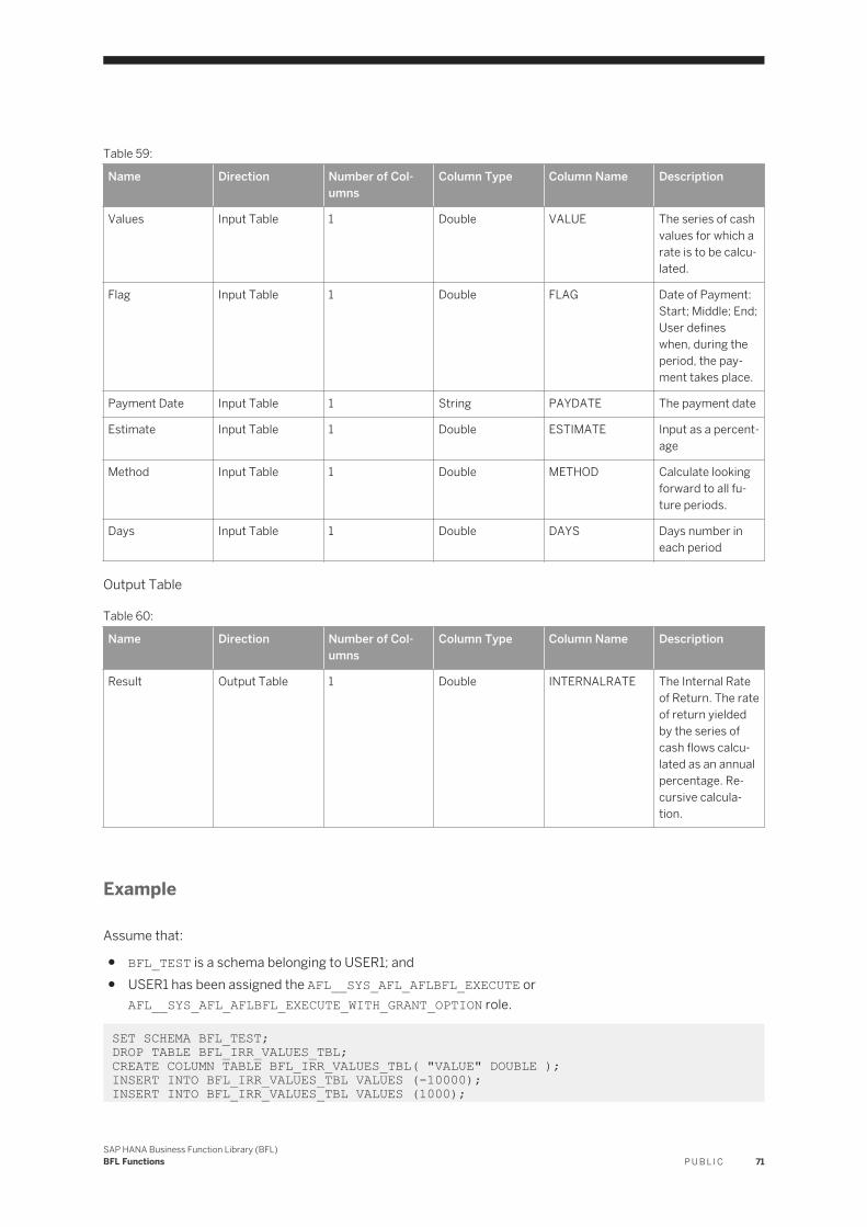
Table 59:
Name Direction Number of Columns
Column Type Column Name Description
Values Input Table 1 Double VALUE The series of cash values for which a rate is to be calculated.
Flag Input Table 1 Double FLAG Date of Payment: Start; Middle; End; User defines when, during the period, the payment takes place.
Payment Date Input Table 1 String PAYDATE The payment date
Estimate Input Table 1 Double ESTIMATE Input as a percentage
Method Input Table 1 Double METHOD Calculate looking forward to all future periods.
Days Input Table 1 Double DAYS Days number in each period
Output Table
Table 60:
Name Direction Number of Columns
Column Type Column Name Description
Result Output Table 1 Double INTERNALRATE The Internal Rate of Return. The rate of return yielded by the series of cash flows calculated as an annual percentage. Recursive calculation.
Example
Assume that:
● BFL_TEST is a schema belonging to USER1; and● USER1 has been assigned the AFL__SYS_AFL_AFLBFL_EXECUTE or
AFL__SYS_AFL_AFLBFL_EXECUTE_WITH_GRANT_OPTION role.
SET SCHEMA BFL_TEST; DROP TABLE BFL_IRR_VALUES_TBL;CREATE COLUMN TABLE BFL_IRR_VALUES_TBL( "VALUE" DOUBLE );INSERT INTO BFL_IRR_VALUES_TBL VALUES (-10000);INSERT INTO BFL_IRR_VALUES_TBL VALUES (1000);
SAP HANA Business Function Library (BFL)BFL Functions P U B L I C 71

INSERT INTO BFL_IRR_VALUES_TBL VALUES (2500);INSERT INTO BFL_IRR_VALUES_TBL VALUES (4000);INSERT INTO BFL_IRR_VALUES_TBL VALUES (4000);INSERT INTO BFL_IRR_VALUES_TBL VALUES (4000);INSERT INTO BFL_IRR_VALUES_TBL VALUES (4000);DROP TABLE BFL_IRR_FLAG_TBL;CREATE COLUMN TABLE BFL_IRR_FLAG_TBL( "FLAG" DOUBLE );INSERT INTO BFL_IRR_FLAG_TBL VALUES (4);INSERT INTO BFL_IRR_FLAG_TBL VALUES (3);INSERT INTO BFL_IRR_FLAG_TBL VALUES (3);INSERT INTO BFL_IRR_FLAG_TBL VALUES (3);INSERT INTO BFL_IRR_FLAG_TBL VALUES (3);INSERT INTO BFL_IRR_FLAG_TBL VALUES (3);INSERT INTO BFL_IRR_FLAG_TBL VALUES (3);DROP TABLE BFL_IRR_USERDATE_TBL;CREATE COLUMN TABLE BFL_IRR_USERDATE_TBL( "PAYDATE" VARCHAR(255) );INSERT INTO BFL_IRR_USERDATE_TBL VALUES ('12/10/00');DROP TABLE BFL_IRR_ESTIMATE_TBL;CREATE COLUMN TABLE BFL_IRR_ESTIMATE_TBL( "ESTIMATE" DOUBLE );INSERT INTO BFL_IRR_ESTIMATE_TBL VALUES (0.3);DROP TABLE BFL_IRR_METHOD_TBL;CREATE COLUMN TABLE BFL_IRR_METHOD_TBL( "METHOD" DOUBLE );INSERT INTO BFL_IRR_METHOD_TBL VALUES (0);INSERT INTO BFL_IRR_METHOD_TBL VALUES (1);INSERT INTO BFL_IRR_METHOD_TBL VALUES (1);INSERT INTO BFL_IRR_METHOD_TBL VALUES (1);INSERT INTO BFL_IRR_METHOD_TBL VALUES (1);INSERT INTO BFL_IRR_METHOD_TBL VALUES (1);INSERT INTO BFL_IRR_METHOD_TBL VALUES (1);DROP TABLE BFL_IRR_DAYS_TBL;CREATE COLUMN TABLE BFL_IRR_DAYS_TBL( "DAYS" DOUBLE );INSERT INTO BFL_IRR_DAYS_TBL VALUES (365);INSERT INTO BFL_IRR_DAYS_TBL VALUES (365);INSERT INTO BFL_IRR_DAYS_TBL VALUES (365);INSERT INTO BFL_IRR_DAYS_TBL VALUES (365);INSERT INTO BFL_IRR_DAYS_TBL VALUES (365);INSERT INTO BFL_IRR_DAYS_TBL VALUES (365);INSERT INTO BFL_IRR_DAYS_TBL VALUES (365);DROP TABLE BFL_IRR_RESULT_TBL;CREATE COLUMN TABLE BFL_IRR_RESULT_TBL( "INTERNALRATE" DOUBLE); CALL _SYS_AFL.AFLBFL_INTERNALRATE_PROC(BFL_IRR_VALUES_TBL, BFL_IRR_FLAG_TBL, BFL_IRR_USERDATE_TBL, BFL_IRR_ESTIMATE_TBL, BFL_IRR_METHOD_TBL, BFL_IRR_DAYS_TBL, BFL_IRR_RESULT_TBL) WITH OVERVIEW; SELECT * FROM BFL_IRR_RESULT_TBL;
3.25 Lag
This function lags an input from one row by a certain number of periods and returns the result in another row. This is a streamlined method for estimating lag periods (such as invoice to receipt) directly into the model.
Formula
The result in period n lags the input by p periods;
(Lag result, period n) = (Input, period n-p)
72 P U B L I CSAP HANA Business Function Library (BFL)
BFL Functions

If the lagged result requires inputs outside the timescale, use the values from parameter Pad.
(Lag result, period n) = (Pad, period n)
Signature
Input Tables
Table 61:
Name Direction Number of Columns
Column Type Column Name Description
Basevalues Input Table 1 Double VALUE Sets a lag of a variable number of periods according to what is contained in the Dimension List item.
Pad Input Table 1 Double PAD Constant to pad values contrast to the corresponding base values.
Periods Input Table 1 Double PERIOD The series to be lagged (e.g. invoiced amounts).
Output Table
Table 62:
Name Direction Number of Columns
Column Type Column Name Description
Result Output Table 1 Double VALUE Lag result (e.g. cash payments made after a lag of n periods).
Example
Assume that:
● BFL_TEST is a schema belonging to USER1; and● USER1 has been assigned the AFL__SYS_AFL_AFLBFL_EXECUTE or
AFL__SYS_AFL_AFLBFL_EXECUTE_WITH_GRANT_OPTION role.
SET SCHEMA BFL_TEST; DROP TABLE BFL_LAG_VALUES_TBL ;CREATE COLUMN TABLE BFL_LAG_VALUES_TBL ( "VALUE" DOUBLE ) ;base valuesINSERT INTO BFL_LAG_VALUES_TBL VALUES (1000);INSERT INTO BFL_LAG_VALUES_TBL VALUES (2000);
SAP HANA Business Function Library (BFL)BFL Functions P U B L I C 73

INSERT INTO BFL_LAG_VALUES_TBL VALUES (2500);INSERT INTO BFL_LAG_VALUES_TBL VALUES (2300);INSERT INTO BFL_LAG_VALUES_TBL VALUES (3000);INSERT INTO BFL_LAG_VALUES_TBL VALUES (1200);DROP TABLE BFL_LAG_PAD_TBL ;CREATE COLUMN TABLE BFL_LAG_PAD_TBL ( "PAD" DOUBLE ) ;INSERT INTO BFL_LAG_PAD_TBL VALUES (999);INSERT INTO BFL_LAG_PAD_TBL VALUES (888);INSERT INTO BFL_LAG_PAD_TBL VALUES (0);INSERT INTO BFL_LAG_PAD_TBL VALUES (0);INSERT INTO BFL_LAG_PAD_TBL VALUES (0);INSERT INTO BFL_LAG_PAD_TBL VALUES (0);DROP TABLE BFL_LAG_PERIOD_TBL ;CREATE COLUMN TABLE BFL_LAG_PERIOD_TBL ( "PERIOD" DOUBLE ) ;INSERT INTO BFL_LAG_PERIOD_TBL VALUES (2);INSERT INTO BFL_LAG_PERIOD_TBL VALUES (2);INSERT INTO BFL_LAG_PERIOD_TBL VALUES (2);INSERT INTO BFL_LAG_PERIOD_TBL VALUES (2);INSERT INTO BFL_LAG_PERIOD_TBL VALUES (2);INSERT INTO BFL_LAG_PERIOD_TBL VALUES (2);DROP TABLE BFL_LAG_RESULTS_TBL ;CREATE COLUMN TABLE BFL_LAG_RESULTS_TBL ( "VALUE" DOUBLE) ; CALL _SYS_AFL.AFLBFL_LAG_PROC(BFL_LAG_VALUES_TBL, BFL_LAG_PAD_TBL, BFL_LAG_PERIOD_TBL, BFL_LAG_RESULTS_TBL) WITH OVERVIEW; SELECT * FROM BFL_LAG_RESULTS_TBL;
3.26 Last
This function returns the most recent non-zero value of the input over a number of periods. When the input changes rarely, it helps to avoid re-entering data.
Formula
The result is the most recent non-zero value of the input in Period n .
Signature
Input Tables
Table 63:
Name Direction Number of Columns
Column Type Column Name Description
Prime Input Table 1 Double VALUE The series of data on which Last operates.
Output Table
74 P U B L I CSAP HANA Business Function Library (BFL)
BFL Functions

Table 64:
Name Direction Number of Columns
Column Type Column Name Description
Result Output Table 1 Double LAST The most recent non-zero value in the series of data to a precision of 1x10^(-12).
Example
Assume that:
● BFL_TEST is a schema belonging to USER1; and● USER1 has been assigned the AFL__SYS_AFL_AFLBFL_EXECUTE or
AFL__SYS_AFL_AFLBFL_EXECUTE_WITH_GRANT_OPTION role.
SET SCHEMA BFL_TEST; DROP TABLE BFL_LAST_PRIME_TBL;CREATE COLUMN TABLE BFL_LAST_PRIME_TBL( "VALUE" DOUBLE );INSERT INTO BFL_LAST_PRIME_TBL VALUES (200);INSERT INTO BFL_LAST_PRIME_TBL VALUES (0);INSERT INTO BFL_LAST_PRIME_TBL VALUES (0);INSERT INTO BFL_LAST_PRIME_TBL VALUES (300);INSERT INTO BFL_LAST_PRIME_TBL VALUES (0);INSERT INTO BFL_LAST_PRIME_TBL VALUES (400);INSERT INTO BFL_LAST_PRIME_TBL VALUES (0);INSERT INTO BFL_LAST_PRIME_TBL VALUES (500);INSERT INTO BFL_LAST_PRIME_TBL VALUES (0);DROP TABLE BFL_LAST_LAST_TBL;CREATE COLUMN TABLE BFL_LAST_LAST_TBL( "LAST" DOUBLE); CALL _SYS_AFL.AFLBFL_LAST_PROC(BFL_LAST_PRIME_TBL, BFL_LAST_LAST_TBL) WITH OVERVIEW; SELECT * FROM BFL_LAST_LAST_TBL;
3.27 Lease
This function calculates a payment schedule (e.g. How much you need to pay in each period) for a lease, loan, mortgage, annuity or savings account. Multiple lease contracts are allowed to be entered on one single page, and the terms of each contract in one single column. This is similar to the Payment Function, but it allows Year over Year Difference leases to be entered in Year over Year Difference columns, as opposed to Year over Year Difference pages.
For each lease, the inputs include annual interest rate, term, present and future values, and the result is a constant payment. Interest, a constant or vary by each period, is entered per period and compounded at the end of each period. Early redemption is allowed, which is a percentage of the opening balance. Lease requires equal, consecutive periods.
Embedded Lease Function is a critical element for accurate CAPEX planning and treasury applications.
SAP HANA Business Function Library (BFL)BFL Functions P U B L I C 75

Signature
Input Tables
Table 65:
Name Direction Number of Columns
Column Type Column Name Description
Advance Amount Input Table 1 Double ADVANCE The payment from or to the account at the start of the calculation. If no further advances occur, leave it as zero.
Residual Amount Input Table 1 Double RESIDUAL The payment from or to account at the end of the calculation. If the account is repaid completely, the loan would be zero.
Number Periods Input Table 1 Double PERIODS The number of periods the account is to run.
When to Pay Input Table 1 Double WHENTOPAY 0 = Payment is made at the end of the period. (Default) 1= Payment is made at the start of the period.
Interest Rate Input Table 1 Double RATE Percentage rate per period.
Redemption Rate Input Table 1 Double REDEMPTIONREATE
Interpreted as a percentage, but it must be the rate per period.
Output Table
Table 66:
Name Direction Number of Columns
Column Type Column Name Description
Result Output Table 10 Double OPENING The opening balance of the account. Will be equal to PRESENT VALUE in the first calculation period.
76 P U B L I CSAP HANA Business Function Library (BFL)
BFL Functions

Name Direction Number of Columns
Column Type Column Name Description
Double ADJUSTED The opening balance of the account adjusted for redemptions and further advances.
Double INTEREST 0 = Adjusted Opening * Rate per Period/100 1 = (Adjusted Opening + Payment) * Rate per Period/100
Double PAYMENT The single payment to the account this period which contains interest element and capital element.
Double REDEMPTION The amount of the account paid off early Calculated by: First period: Advance Amount* Redemption Rate /100 Subsequent periods: (Opening Value)* Redemption Rate /100
Double CAPITAL The amount of capital paid off in the period
Double RESIDUALPAIDOFF
Will be non-zero only in the last period of the account when it represents the residual value of the loan being repaid. It is equal to FUTURE VALUE from the first period adjusted by any redemptions during the life of the loan.
Double CLOSING The closing balance of the account. Should be set as a time average, last period.
SAP HANA Business Function Library (BFL)BFL Functions P U B L I C 77

Name Direction Number of Columns
Column Type Column Name Description
Double PERIODSREMAINING
Will be the Number of periods in the first calculation period and will reduce by 1 in each subsequent period.
Double CALCRESIDUAL FUTURE VALUE from the first period adjusted by redemptions during the life of the loan to date.
Example
Assume that:
● BFL_TEST is a schema belonging to USER1; and● USER1 has been assigned the AFL__SYS_AFL_AFLBFL_EXECUTE or
AFL__SYS_AFL_AFLBFL_EXECUTE_WITH_GRANT_OPTION role.
SET SCHEMA BFL_TEST; DROP TABLE BFL_LEASE_ADVANCE_TBL ;CREATE COLUMN TABLE BFL_LEASE_ADVANCE_TBL ( "ADVANCE" DOUBLE );INSERT INTO BFL_LEASE_ADVANCE_TBL VALUES (150000) ;INSERT INTO BFL_LEASE_ADVANCE_TBL VALUES (0) ;INSERT INTO BFL_LEASE_ADVANCE_TBL VALUES (0) ;INSERT INTO BFL_LEASE_ADVANCE_TBL VALUES (0) ;DROP TABLE BFL_LEASE_RESIDUAL_TBL ;CREATE COLUMN TABLE BFL_LEASE_RESIDUAL_TBL ( "RESIDUAL" DOUBLE ) ;INSERT INTO BFL_LEASE_RESIDUAL_TBL VALUES (10000) ;INSERT INTO BFL_LEASE_RESIDUAL_TBL VALUES (0) ;INSERT INTO BFL_LEASE_RESIDUAL_TBL VALUES (0) ;INSERT INTO BFL_LEASE_RESIDUAL_TBL VALUES (0) ;DROP TABLE BFL_LEASE_PERIODS_TBL ;CREATE COLUMN TABLE BFL_LEASE_PERIODS_TBL ( "PERIODS" DOUBLE ) ;INSERT INTO BFL_LEASE_PERIODS_TBL VALUES (4) ;INSERT INTO BFL_LEASE_PERIODS_TBL VALUES (0) ;INSERT INTO BFL_LEASE_PERIODS_TBL VALUES (0) ;INSERT INTO BFL_LEASE_PERIODS_TBL VALUES (0) ;DROP TABLE BFL_LEASE_WHENTOPAY_TBL ;CREATE COLUMN TABLE BFL_LEASE_WHENTOPAY_TBL ( "WHENTOPAY" DOUBLE ) ;INSERT INTO BFL_LEASE_WHENTOPAY_TBL VALUES (1) ;INSERT INTO BFL_LEASE_WHENTOPAY_TBL VALUES (1) ;INSERT INTO BFL_LEASE_WHENTOPAY_TBL VALUES (1) ;INSERT INTO BFL_LEASE_WHENTOPAY_TBL VALUES (1) ;DROP TABLE BFL_LEASE_RATE_TBL ;CREATE COLUMN TABLE BFL_LEASE_RATE_TBL ( "RATE" DOUBLE ) ;INSERT INTO BFL_LEASE_RATE_TBL VALUES (0.02) ;INSERT INTO BFL_LEASE_RATE_TBL VALUES (0.015) ;INSERT INTO BFL_LEASE_RATE_TBL VALUES (0.015) ;INSERT INTO BFL_LEASE_RATE_TBL VALUES (0.015) ;DROP TABLE BFL_LEASE_REDEMPTIONREATE_TBL ;CREATE COLUMN TABLE BFL_LEASE_REDEMPTIONREATE_TBL ( "REDEMPTIONREATE" DOUBLE ) ;
78 P U B L I CSAP HANA Business Function Library (BFL)
BFL Functions

INSERT INTO BFL_LEASE_REDEMPTIONREATE_TBL VALUES (0) ;INSERT INTO BFL_LEASE_REDEMPTIONREATE_TBL VALUES (0) ;INSERT INTO BFL_LEASE_REDEMPTIONREATE_TBL VALUES (0) ;INSERT INTO BFL_LEASE_REDEMPTIONREATE_TBL VALUES (0) ;DROP TABLE BFL_LEASE_RESULTS_TBL ; CREATE COLUMN TABLE BFL_LEASE_RESULTS_TBL( "OPENING" DOUBLE, "ADJUSTED" DOUBLE, "INTEREST" DOUBLE, "PAYMENT" DOUBLE, "REDEMPTION" DOUBLE, "CAPITAL" DOUBLE, "RESIDUALPAIDOFF" DOUBLE, "CLOSING" DOUBLE, "PERIODSREMAINING" DOUBLE, "CALCRESIDUAL" DOUBLE) ; CALL _SYS_AFL.AFLBFL_LEASE_PROC(BFL_LEASE_ADVANCE_TBL, BFL_LEASE_RESIDUAL_TBL, BFL_LEASE_PERIODS_TBL, BFL_LEASE_WHENTOPAY_TBL, BFL_LEASE_RATE_TBL, BFL_LEASE_REDEMPTIONREATE_TBL, BFL_LEASE_RESULTS_TBL) WITH OVERVIEW; SELECT * FROM BFL_LEASE_RESULTS_TBL ;
3.28 Lease Variable
This function calculates a payment schedule along a time scale (life of the loan). The time scale requires equal and consecutive periods. In each period, a single payment must be made according to the When to Pay parameter. It is not necessary to compound the interest in each period.
Compared with the Lease function, Lease Variable has two more input columns which represent two more parameters: Compound and Recalculate.
● Compound: indicates whether or not to calculate compound interest in this period.● Recalculate: determines whether or not to recalculate the payment schedule to take account of interest
rate changes or other changes during this period.
Signature
Input Tables
Table 67:
Name Direction Number of Columns
Column Type Column Name Description
Advance Amount Input Table 1 Double ADVANCE The payment from or to the account at the start of the calculation. If no further advances occur, leave it as zero.
SAP HANA Business Function Library (BFL)BFL Functions P U B L I C 79

Name Direction Number of Columns
Column Type Column Name Description
Residual Amount Input Table 1 Double RESIDUAL The payment from or to account at the end of the calculation. If the account is repaid completely, the loan would be zero.
Number Periods Input Table 1 Double PERIODS The number of periods the account is to run.
When to Pay Input Table 1 Double WHENTOPAY 0 = Payment is made at the end of the period. (Default) 1= Payment is made at the start of the period.
Interest Rate Input Table 1 Double RATE Percentage rate per period.
Redemption Rate Input Table 1 Double REDEMPTIONREATE
Interpreted as a percentage but must be the rate per period.
Compound Input Table 1 Double COMPOUND Indicate whether or not to compound interest this period.
Recalculate Input Table 1 Double RECALCULATE Indicate whether or not to recalculate payments to take account of interest rate changes during this period.
Output Table
Table 68:
Name Direction Number of Columns
Column Type Column Name Description
Result Output Table 11 Double OPENING The opening balance of the account. Will be equal to PRESENT VALUE in the first calculation period.
80 P U B L I CSAP HANA Business Function Library (BFL)
BFL Functions

Name Direction Number of Columns
Column Type Column Name Description
Double ADJUSTED The opening balance of the account adjusted for redemptions and further advances.
Double INTEREST 0 = Adjusted Opening * Rate per Period/100. 1 = (Adjusted Opening + Payment) * Rate per Period/100.
Double ACCRUED Any interest calculated in previous periods not yet applied to the account.
Double PAYMENT The single payment to the account this period which contains interest element and capital element.
Double REDEMPTION The amount of the account paid off early Calculated by: First Period: Advance Amount* Redemption Rate /100 Subsequent periods: (Opening Value)* Redemption Rate /100
Double CAPITAL The amount of capital paid off in the period
Double RESIDUALPAIDOFF
Will be non-zero only in the last period of the account when it represents the residual value of the loan being repaid. It is equal to FUTURE VALUE from the first period adjusted by any redemptions during the life of the loan.
SAP HANA Business Function Library (BFL)BFL Functions P U B L I C 81

Name Direction Number of Columns
Column Type Column Name Description
Double CLOSING The closing balance of the account. Should be set as a time average, last period.
Double PERIODSREMAINING
Will be Number of periods in the first calculation period and will reduce by 1 in each subsequent period.
Double CALCRESIDUAL FUTURE VALUE from the first period adjusted by redemptions during the life of the loan to date.
Example
Assume that:
● BFL_TEST is a schema belonging to USER1; and● USER1 has been assigned the AFL__SYS_AFL_AFLBFL_EXECUTE or
AFL__SYS_AFL_AFLBFL_EXECUTE_WITH_GRANT_OPTION role.
SET SCHEMA BFL_TEST; DROP TABLE BFL_LSVB_ADVANCE_TBL ;CREATE COLUMN TABLE BFL_LSVB_ADVANCE_TBL ( "ADVANCE" DOUBLE );INSERT INTO BFL_LSVB_ADVANCE_TBL VALUES (100000) ;INSERT INTO BFL_LSVB_ADVANCE_TBL VALUES (0) ;INSERT INTO BFL_LSVB_ADVANCE_TBL VALUES (0) ;INSERT INTO BFL_LSVB_ADVANCE_TBL VALUES (0) ;INSERT INTO BFL_LSVB_ADVANCE_TBL VALUES (0) ;INSERT INTO BFL_LSVB_ADVANCE_TBL VALUES (0) ;DROP TABLE BFL_LSVB_RESIDUAL_TBL ;CREATE COLUMN TABLE BFL_LSVB_RESIDUAL_TBL ( "RESIDUAL" DOUBLE ) ;INSERT INTO BFL_LSVB_RESIDUAL_TBL VALUES (15000) ;INSERT INTO BFL_LSVB_RESIDUAL_TBL VALUES (0) ;INSERT INTO BFL_LSVB_RESIDUAL_TBL VALUES (0) ;INSERT INTO BFL_LSVB_RESIDUAL_TBL VALUES (0) ;INSERT INTO BFL_LSVB_RESIDUAL_TBL VALUES (0) ;INSERT INTO BFL_LSVB_RESIDUAL_TBL VALUES (0) ;DROP TABLE BFL_LSVB_PERIODS_TBL ;CREATE COLUMN TABLE BFL_LSVB_PERIODS_TBL ( "PERIODS" DOUBLE ) ;INSERT INTO BFL_LSVB_PERIODS_TBL VALUES (6) ;INSERT INTO BFL_LSVB_PERIODS_TBL VALUES (0) ;INSERT INTO BFL_LSVB_PERIODS_TBL VALUES (0) ;INSERT INTO BFL_LSVB_PERIODS_TBL VALUES (0) ;INSERT INTO BFL_LSVB_PERIODS_TBL VALUES (0) ;INSERT INTO BFL_LSVB_PERIODS_TBL VALUES (0) ;DROP TABLE BFL_LSVB_WHENTOPAY_TBL ;CREATE COLUMN TABLE BFL_LSVB_WHENTOPAY_TBL ( "WHENTOPAY" DOUBLE ) ;INSERT INTO BFL_LSVB_WHENTOPAY_TBL VALUES (1) ;
82 P U B L I CSAP HANA Business Function Library (BFL)
BFL Functions

INSERT INTO BFL_LSVB_WHENTOPAY_TBL VALUES (1) ;INSERT INTO BFL_LSVB_WHENTOPAY_TBL VALUES (1) ;INSERT INTO BFL_LSVB_WHENTOPAY_TBL VALUES (1) ;INSERT INTO BFL_LSVB_WHENTOPAY_TBL VALUES (1) ;INSERT INTO BFL_LSVB_WHENTOPAY_TBL VALUES (1) ;DROP TABLE BFL_LSVB_RATE_TBL ;CREATE COLUMN TABLE BFL_LSVB_RATE_TBL ( "RATE" DOUBLE ) ;INSERT INTO BFL_LSVB_RATE_TBL VALUES (0.01) ;INSERT INTO BFL_LSVB_RATE_TBL VALUES (0.01) ;INSERT INTO BFL_LSVB_RATE_TBL VALUES (0.01) ;INSERT INTO BFL_LSVB_RATE_TBL VALUES (0.01) ;INSERT INTO BFL_LSVB_RATE_TBL VALUES (0.01) ;INSERT INTO BFL_LSVB_RATE_TBL VALUES (0.01) ;DROP TABLE BFL_LSVB_REDEMPTIONREATE_TBL ;CREATE COLUMN TABLE BFL_LSVB_REDEMPTIONREATE_TBL ( "REDEMPTIONREATE" DOUBLE ) ;INSERT INTO BFL_LSVB_REDEMPTIONREATE_TBL VALUES (0) ;INSERT INTO BFL_LSVB_REDEMPTIONREATE_TBL VALUES (0) ;INSERT INTO BFL_LSVB_REDEMPTIONREATE_TBL VALUES (0) ;INSERT INTO BFL_LSVB_REDEMPTIONREATE_TBL VALUES (0) ;INSERT INTO BFL_LSVB_REDEMPTIONREATE_TBL VALUES (0) ;INSERT INTO BFL_LSVB_REDEMPTIONREATE_TBL VALUES (0) ;DROP TABLE BFL_LSVB_COMPOUND_TBL ;CREATE COLUMN TABLE BFL_LSVB_COMPOUND_TBL ( "COMPOUND" DOUBLE ) ;INSERT INTO BFL_LSVB_COMPOUND_TBL VALUES (2) ;INSERT INTO BFL_LSVB_COMPOUND_TBL VALUES (2) ;INSERT INTO BFL_LSVB_COMPOUND_TBL VALUES (2) ;INSERT INTO BFL_LSVB_COMPOUND_TBL VALUES (2) ;INSERT INTO BFL_LSVB_COMPOUND_TBL VALUES (2) ;INSERT INTO BFL_LSVB_COMPOUND_TBL VALUES (2) ;DROP TABLE BFL_LSVB_RECALCULATE_TBL ;CREATE COLUMN TABLE BFL_LSVB_RECALCULATE_TBL ( "RECALCULATE" DOUBLE ) ;INSERT INTO BFL_LSVB_RECALCULATE_TBL VALUES (2) ;INSERT INTO BFL_LSVB_RECALCULATE_TBL VALUES (2) ;INSERT INTO BFL_LSVB_RECALCULATE_TBL VALUES (2) ;INSERT INTO BFL_LSVB_RECALCULATE_TBL VALUES (2) ;INSERT INTO BFL_LSVB_RECALCULATE_TBL VALUES (2) ;INSERT INTO BFL_LSVB_RECALCULATE_TBL VALUES (2) ;DROP TABLE BFL_LSVB_RESULTS_TBL ; CREATE COLUMN TABLE BFL_LSVB_RESULTS_TBL( "OPENING" DOUBLE, "ADJUSTED" DOUBLE, "INTEREST" DOUBLE,"ACCRUED" DOUBLE, "PAYMENT" DOUBLE, "REDEMPTION" DOUBLE, "CAPITAL" DOUBLE, "RESIDUALPAIDOFF" DOUBLE, "CLOSING" DOUBLE, "PERIODSREMAINING" DOUBLE, "CALCRESIDUAL" DOUBLE) ; CALL _SYS_AFL.AFLBFL_LEASEVARIABLE_PROC(BFL_LSVB_ADVANCE_TBL, BFL_LSVB_RESIDUAL_TBL, BFL_LSVB_PERIODS_TBL, BFL_LSVB_WHENTOPAY_TBL, BFL_LSVB_RATE_TBL, BFL_LSVB_REDEMPTIONREATE_TBL, BFL_LSVB_COMPOUND_TBL, BFL_LSVB_RECALCULATE_TBL, BFL_LSVB_RESULTS_TBL) WITH OVERVIEW; SELECT * FROM BFL_LSVB_RESULTS_TBL ;
3.29 Linear Average
This function calculates a linear average, in which larger weights are applied to more recent periods. The weights decrease linearly as you look back over time.
SAP HANA Business Function Library (BFL)BFL Functions P U B L I C 83

Formula
Where: Avg(n)= the average for the nth period
Orig(i)= original data for ith period
Signature
Input Tables
Table 69:
Name Direction Number of Columns
Column Type Column Name Description
Sales Input Table 1 Double VALUE The original series to be averaged (sales)
Output Table
Table 70:
Name Direction Number of Columns
Column Type Column Name Description
Result Output Table 1 Double AVERAGED_RESULT
The linear average (average sales)
Example
Assume that:
● BFL_TEST is a schema belonging to USER1; and● USER1 has been assigned the AFL__SYS_AFL_AFLBFL_EXECUTE or
AFL__SYS_AFL_AFLBFL_EXECUTE_WITH_GRANT_OPTION role.
SET SCHEMA BFL_TEST; DROP TABLE BFL_LA_SALES_TBL;CREATE COLUMN TABLE BFL_LA_SALES_TBL( "VALUE" DOUBLE );INSERT INTO BFL_LA_SALES_TBL VALUES (1000) ;INSERT INTO BFL_LA_SALES_TBL VALUES (2000) ;INSERT INTO BFL_LA_SALES_TBL VALUES (1500) ;INSERT INTO BFL_LA_SALES_TBL VALUES (2200) ;INSERT INTO BFL_LA_SALES_TBL VALUES (1750) ;INSERT INTO BFL_LA_SALES_TBL VALUES (2000) ;DROP TABLE BFL_LA_AVERGAESALES_TBL;
84 P U B L I CSAP HANA Business Function Library (BFL)
BFL Functions

CREATE COLUMN TABLE BFL_LA_AVERGAESALES_TBL( "AVERAGED_RESULT" DOUBLE) ; CALL _SYS_AFL.AFLBFL_LINEARAVERAGE_PROC(BFL_LA_SALES_TBL, BFL_LA_AVERGAESALES_TBL) WITH OVERVIEW ; SELECT * FROM BFL_LA_AVERGAESALES_TBL ;
3.30 Max Value
This function returns the maximum value of a specific field of items.
Signature
Input Tables
Table 71:
Name Direction Number of Columns
Column Type Column Name Description
Value Input Table 1 Double VALUE Identifies the items that the maximum is taken over
Output Table
Table 72:
Name Direction Number of Columns
Column Type Column Name Description
Result Output Table 1 Double MAX_MIXVALUE The maximum value for the selected items
Input Flag
Table 73:
Name Direction Value Type Description
Flag Input Value 1 Int Specifies this as Max function, corresponding to Min Function
Example
Assume that:
SAP HANA Business Function Library (BFL)BFL Functions P U B L I C 85
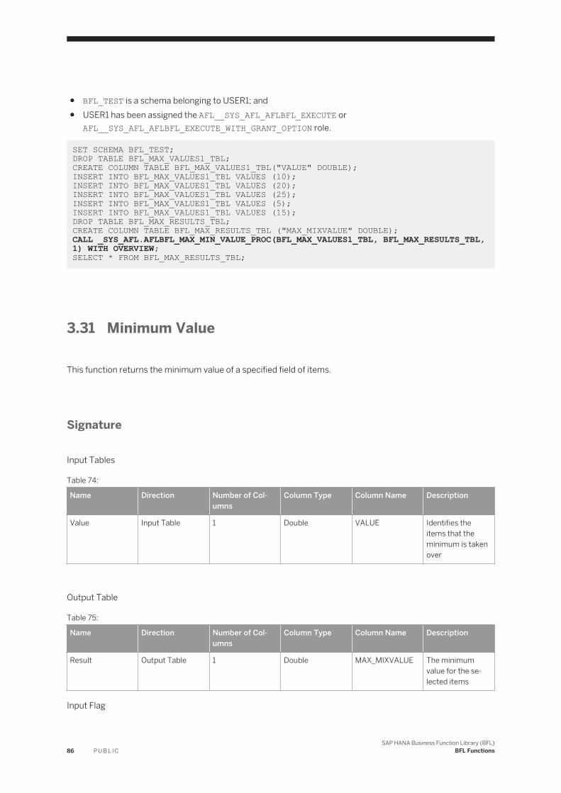
● BFL_TEST is a schema belonging to USER1; and● USER1 has been assigned the AFL__SYS_AFL_AFLBFL_EXECUTE or
AFL__SYS_AFL_AFLBFL_EXECUTE_WITH_GRANT_OPTION role.
SET SCHEMA BFL_TEST; DROP TABLE BFL_MAX_VALUES1_TBL;CREATE COLUMN TABLE BFL_MAX_VALUES1_TBL("VALUE" DOUBLE);INSERT INTO BFL_MAX_VALUES1_TBL VALUES (10);INSERT INTO BFL_MAX_VALUES1_TBL VALUES (20);INSERT INTO BFL_MAX_VALUES1_TBL VALUES (25);INSERT INTO BFL_MAX_VALUES1_TBL VALUES (5);INSERT INTO BFL_MAX_VALUES1_TBL VALUES (15);DROP TABLE BFL_MAX_RESULTS_TBL;CREATE COLUMN TABLE BFL_MAX_RESULTS_TBL ("MAX_MIXVALUE" DOUBLE); CALL _SYS_AFL.AFLBFL_MAX_MIN_VALUE_PROC(BFL_MAX_VALUES1_TBL, BFL_MAX_RESULTS_TBL,1) WITH OVERVIEW; SELECT * FROM BFL_MAX_RESULTS_TBL;
3.31 Minimum Value
This function returns the minimum value of a specified field of items.
Signature
Input Tables
Table 74:
Name Direction Number of Columns
Column Type Column Name Description
Value Input Table 1 Double VALUE Identifies the items that the minimum is taken over
Output Table
Table 75:
Name Direction Number of Columns
Column Type Column Name Description
Result Output Table 1 Double MAX_MIXVALUE The minimum value for the selected items
Input Flag
86 P U B L I CSAP HANA Business Function Library (BFL)
BFL Functions

Table 76:
Name Direction Value Type Description
Flag Input Value 0 Int Specifies this as Min function, corresponding to Max Function
Example
Assume that:
● BFL_TEST is a schema belonging to USER1; and● USER1 has been assigned the AFL__SYS_AFL_AFLBFL_EXECUTE or
AFL__SYS_AFL_AFLBFL_EXECUTE_WITH_GRANT_OPTION role.
SET SCHEMA BFL_TEST; DROP TABLE BFL_MIN_VALUES1_TBL;CREATE COLUMN TABLE BFL_MIN_VALUES1_TBL("VALUE" DOUBLE);INSERT INTO BFL_MIN_VALUES1_TBL VALUES (10);INSERT INTO BFL_MIN_VALUES1_TBL VALUES (20);INSERT INTO BFL_MIN_VALUES1_TBL VALUES (25);INSERT INTO BFL_MIN_VALUES1_TBL VALUES (5);INSERT INTO BFL_MIN_VALUES1_TBL VALUES (15);DROP TABLE BFL_MIN_RESULTS_TBL;CREATE COLUMN TABLE BFL_MIN_RESULTS_TBL ("MAX_MIXVALUE" DOUBLE); CALL _SYS_AFL.AFLBFL_MAX_MIN_VALUE_PROC(BFL_MIN_VALUES1_TBL, BFL_MIN_RESULTS_TBL,0) WITH OVERVIEW; SELECT * FROM BFL_MIN_RESULTS_TBL;
3.32 Moving Average&Moving Sum
This function needs to use the generator mentioned in Calling BFL Functions [page 7].
These two built-in functions calculate a moving average or moving sum over a specified number of periods.
Formula
The formula for Moving Average is:
Moving Average = Sum of Originals over n periods/ Number of periods to be averaged
The formula for Moving Sum is:
Moving Sum = Sum of Originals over n periods
The relationship between the Moving Sum S and the Moving Average A is:
SAP HANA Business Function Library (BFL)BFL Functions P U B L I C 87

S=A*length
where length is the length of the moving average.
The choice of which originals to include in the formula depends on the style of average and the method of dealing with end conditions for missing data.
Methods R for replicate and L for linear extrapolation estimate the values for the missing periods. Methods P for prime, T for take, U for unequal, and W for weightings estimate the result directly.
Replicate: The first and last original periods are replicated as many times as needed. This is the simplest rule and is used as the default if you do not specify another method.
Linear extrapolation: The missing n periods at the front of the original series are provided by extending the line joining the centers of the first and second set of n periods of the original series. The missing periods at the back are provided in the same way by extending the line joining the last two sets of n input periods to the right.
Prime: Get the unavailable averages from another variable. This is typically a constant (e.g. zero), as strictly speaking the data is not available, but if you know the missing data you can enter it here in the Prime variable.
Take: Takes an average over as many periods as there is data available but does not extrapolate or estimate any further. For example, using a 3 period last average style (L3) with method T for the end conditions would give an average of (Jan/1) in Jan, (Jan+Feb)/2 in Feb and (Jan+Feb+Mar)/3 in Mar. Method T is not permitted with style W.
Unequal: Calculates separate right and left averages using the largest average available and then averages the two averages. This is a better variant of the "T for Take" method for the centered styles C. For styles F and L method U is the same as method T. The central period is shared between the two averages. Method U is not permitted with style W.
Weights: This option gives you the flexibility to provide appropriate weights for the data being averaged/summed. A set of weights is provided for each missing average or sum for styles L and F. For the centered styles C and W, a set of weights is provided for half of the series, the same weights being used to fill the front and the back of the smoothed series.
Signature
Input Tables
88 P U B L I CSAP HANA Business Function Library (BFL)
BFL Functions

Table 77:
Name Direction Number of Columns
Column Type Column Name Description
Original Input Table 1 Double ORIGINAL The original series to be averaged or summed.
Average Style Input Table 1 Double AVERAGESTYLE Last Periods(0): Apply to number of previous periods. Center(1): The average is returned in the center of the n periods averaged. Weightings(2): Weightings specify the weighting applied to each period. (i.e. 1,2,1 for 3 periods)
SAP HANA Business Function Library (BFL)BFL Functions P U B L I C 89

Name Direction Number of Columns
Column Type Column Name Description
Average Method Input Table 1 Double AVERAGEMETHOD
Method describes how to fill the periods at the start and end for which data is missing. Replicate(0): Replicate the first and/or last input periods as many times as needed. Prime input(1): Prime input variable is used to provide the missing averages that cannot be calculated because the original data is not available. This also applies to Estimating. Truncated or Take(2): Truncated sums required are scaled up to carry their full weight. For example, if you are calculating a 5 period sum but only 3 periods are available, it will be scaled up by a factor of 5/3. Unequal length(3): Unequal length averages. Unequal=(Left+Right)/2 using the full length on the side where it is available, and the longest available on the other side. Weighted Replacement(4): Weights provided in formula to calculate missing inputs.
Prime Input Table 1 Double PRIME The original series to be averaged or summed.
90 P U B L I CSAP HANA Business Function Library (BFL)
BFL Functions

Name Direction Number of Columns
Column Type Column Name Description
Average Periods Input Table 1 Double AVERAGEPERIODS
Periods to be calculated.
Weightings Input Table 1~N Double WEIGHTING1~ WEIGHTINGN
Weightings specify the weighting applied to each period. (i.e. 1,2,1 for 3 periods).
Output Table
Table 78:
Name Direction Number of Columns
Column Type Column Name Description
Result Output Table 1 Double RESULTS The moving average or sum over n periods.
Example
Assume that:
● BFL_TEST is a schema belonging to USER1; and● USER1 has been assigned the AFLPM_CREATOR_ERASER_EXECUTE role; and● USER1 has been assigned the AFL__SYS_AFL_AFLBFL_EXECUTE or
AFL__SYS_AFL_AFLBFL_EXECUTE_WITH_GRANT_OPTION role.
SET SCHEMA BFL_TEST; DROP TYPE BFL_MAMS_ORIGINAL_T ;CREATE TYPE BFL_MAMS_ORIGINAL_T AS TABLE( "ORIGINAL" DOUBLE ) ;DROP TYPE BFL_MAMS_AVERAGESTYLE_T ;CREATE TYPE BFL_MAMS_AVERAGESTYLE_T AS TABLE( "AVERAGESTYLE" DOUBLE ) ;DROP TYPE BFL_MAMS_AVERAGEMETHOD_T ;CREATE TYPE BFL_MAMS_AVERAGEMETHOD_T AS TABLE( "AVERAGEMETHOD" DOUBLE ) ;DROP TYPE BFL_MAMS_PRIME_T ;CREATE TYPE BFL_MAMS_PRIME_T AS TABLE( "PRIME" DOUBLE ) ;DROP TYPE BFL_MAMS_AVERAGEPERIODS_T ;CREATE TYPE BFL_MAMS_AVERAGEPERIODS_T AS TABLE( "AVERAGEPERIODS" DOUBLE ) ;DROP TYPE BFL_MAMS_WEIGHTINGS_T ;CREATE TYPE BFL_MAMS_WEIGHTINGS_T AS TABLE( "WEIGHTING1" DOUBLE,"WEIGHTING2" DOUBLE, "WEIGHTING3" DOUBLE) ;DROP TYPE BFL_MAMS_RESULT_T;CREATE TYPE BFL_MAMS_RESULT_T AS TABLE("RESULTS" DOUBLE) ;DROP table BFL_MAMS_PDATA_TBL;CREATE column table BFL_MAMS_PDATA_TBL("POSITION" INT,"SCHEMA_NAME" NVARCHAR(256),"TYPE_NAME" NVARCHAR(256), ”PARAMETER_TYPE” VARCHAR(7));insert into BFL_MAMS_PDATA_TBL values (1,'BFL_TEST’,’BFL_MAMS_ORIGINAL_T', 'IN'); insert into BFL_MAMS_PDATA_TBL values (2,'BFL_TEST’,’BFL_MAMS_AVERAGESTYLE_T', 'IN');insert into BFL_MAMS_PDATA_TBL values (3,'BFL_TEST’,’BFL_MAMS_AVERAGEMETHOD_T', 'IN');insert into BFL_MAMS_PDATA_TBL values (4,'BFL_TEST’,’BFL_MAMS_PRIME_T', 'IN');insert into BFL_MAMS_PDATA_TBL values (5,'BFL_TEST’,’BFL_MAMS_AVERAGEPERIODS_T', 'IN');
SAP HANA Business Function Library (BFL)BFL Functions P U B L I C 91

insert into BFL_MAMS_PDATA_TBL values (6,'BFL_TEST’,’BFL_MAMS_WEIGHTINGS_T', 'IN');insert into BFL_MAMS_PDATA_TBL values (7,'BFL_TEST’,’BFL_MAMS_RESULT_T', 'OUT'); call SYS.AFLLANG_WRAPPER_PROCEDURE_DROP('BFL_TEST’,'AFLBFL_MOVINGAVERAGEANDSUM_PROC'); call SYS.AFLLANG_WRAPPER_PROCEDURE_CREATE('AFLBFL','MOVINGAVERAGEANDSUM','TEST_BFL', 'AFLBFL_MOVINGAVERAGEANDSUM_PROC',BFL_MAMS_PDATA_TBL); DROP TABLE BFL_MAMS_ORIGINAL_TBL ;CREATE COLUMN TABLE BFL_MAMS_ORIGINAL_TBL ( "ORIGINAL" DOUBLE );INSERT INTO BFL_MAMS_ORIGINAL_TBL VALUES (1000) ;INSERT INTO BFL_MAMS_ORIGINAL_TBL VALUES (2000) ;INSERT INTO BFL_MAMS_ORIGINAL_TBL VALUES (3000) ;INSERT INTO BFL_MAMS_ORIGINAL_TBL VALUES (2000) ;INSERT INTO BFL_MAMS_ORIGINAL_TBL VALUES (2000) ;INSERT INTO BFL_MAMS_ORIGINAL_TBL VALUES (8000) ;INSERT INTO BFL_MAMS_ORIGINAL_TBL VALUES (6000) ;INSERT INTO BFL_MAMS_ORIGINAL_TBL VALUES (8000) ;INSERT INTO BFL_MAMS_ORIGINAL_TBL VALUES (7000) ;INSERT INTO BFL_MAMS_ORIGINAL_TBL VALUES (10000) ;INSERT INTO BFL_MAMS_ORIGINAL_TBL VALUES (1000) ;INSERT INTO BFL_MAMS_ORIGINAL_TBL VALUES (9000) ;DROP TABLE BFL_MAMS_AVERAGESTYLE_TBL ;CREATE COLUMN TABLE BFL_MAMS_AVERAGESTYLE_TBL ( "AVERAGESTYLE" DOUBLE ) ;INSERT INTO BFL_MAMS_AVERAGESTYLE_TBL VALUES (2) ;DROP TABLE BFL_MAMS_AVERAGEMETHOD_TBL ;CREATE COLUMN TABLE BFL_MAMS_AVERAGEMETHOD_TBL ( "AVERAGEMETHOD" DOUBLE ) ;INSERT INTO BFL_MAMS_AVERAGEMETHOD_TBL VALUES (0) ;DROP TABLE BFL_MAMS_PRIME_TBL ;CREATE COLUMN TABLE BFL_MAMS_PRIME_TBL ( "PRIME" DOUBLE ) ;INSERT INTO BFL_MAMS_PRIME_TBL VALUES (1000) ;DROP TABLE BFL_MAMS_AVERAGEPERIODS_TBL ;CREATE COLUMN TABLE BFL_MAMS_AVERAGEPERIODS_TBL ( "AVERAGEPERIODS" DOUBLE ) ;INSERT INTO BFL_MAMS_AVERAGEPERIODS_TBL VALUES (3) ;DROP TABLE BFL_MAMS_WEIGHTINGS_TBL ;CREATE COLUMN TABLE BFL_MAMS_WEIGHTINGS_TBL ( "WEIGHTING1" DOUBLE,"WEIGHTING2" DOUBLE, "WEIGHTING3" DOUBLE) ;INSERT INTO BFL_MAMS_WEIGHTINGS_TBL VALUES (1, 2, 1) ;DROP TABLE RESULTS_TBL ;CREATE COLUMN TABLE BFL_MAMS_RESULTS_TBL("RESULTS" DOUBLE) ; CALL BFL_TEST.AFLBFL_MOVINGAVERAGEANDSUM_PROC(BFL_MAMS_ORIGINAL_TBL, BFL_MAMS_AVERAGESTYLE_TBL, BFL_MAMS_AVERAGEMETHOD_TBL, BFL_MAMS_PRIME_TBL, BFL_MAMS_AVERAGEPERIODS_TBL, BFL_MAMS_WEIGHTINGS_TBL, BFL_MAMS_RESULTS_TBL) WITH OVERVIEW; SELECT * FROM BFL_MAMS_RESULTS_TBL ;
3.33 Moving Median
This function sorts the entire input values into ascending sequence and takes the median value. If the number of input values is even, it takes the average of the middle two numbers.
Signature
Input Tables
92 P U B L I CSAP HANA Business Function Library (BFL)
BFL Functions

Table 79:
Name Direction Number of Columns
Column Type Column Name Description
Value Input Table 1 Double VALUE The variable whose median is required
Length Input Table 1 Double LENGTH Number of periods over which to take the median
Offset Input Table 1 Double OFFSET The number of periods offset from the center
Exclude Input Table 1 Double EXCLUDE 0=Include; 1=Exclude
Output Table
Table 80:
Name Direction Number of Columns
Column Type Column Name Description
Result Output Table 1 Double RESULTS The median
Example
Assume that:
● BFL_TEST is a schema belonging to USER1; and● USER1 has been assigned the AFL__SYS_AFL_AFLBFL_EXECUTE or
AFL__SYS_AFL_AFLBFL_EXECUTE_WITH_GRANT_OPTION role.
SET SCHEMA BFL_TEST;DROP TABLE BFL_MVMD_VALUE_TBL ;CREATE COLUMN TABLE BFL_MVMD_VALUE_TBL ( "VALUE" DOUBLE );INSERT INTO BFL_MVMD_VALUE_TBL VALUES (1) ;INSERT INTO BFL_MVMD_VALUE_TBL VALUES (2) ;INSERT INTO BFL_MVMD_VALUE_TBL VALUES (3) ;INSERT INTO BFL_MVMD_VALUE_TBL VALUES (4) ;INSERT INTO BFL_MVMD_VALUE_TBL VALUES (5) ;INSERT INTO BFL_MVMD_VALUE_TBL VALUES (6) ;INSERT INTO BFL_MVMD_VALUE_TBL VALUES (7) ;INSERT INTO BFL_MVMD_VALUE_TBL VALUES (8) ;INSERT INTO BFL_MVMD_VALUE_TBL VALUES (9) ;INSERT INTO BFL_MVMD_VALUE_TBL VALUES (10) ;INSERT INTO BFL_MVMD_VALUE_TBL VALUES (11) ;INSERT INTO BFL_MVMD_VALUE_TBL VALUES (12) ;INSERT INTO BFL_MVMD_VALUE_TBL VALUES (13) ;DROP TABLE BFL_MVMD_LENGTH_TBL ;CREATE COLUMN TABLE BFL_MVMD_LENGTH_TBL ( "LENGTH" DOUBLE ) ;INSERT INTO BFL_MVMD_LENGTH_TBL VALUES (6) ;INSERT INTO BFL_MVMD_LENGTH_TBL VALUES (6) ;INSERT INTO BFL_MVMD_LENGTH_TBL VALUES (6) ;INSERT INTO BFL_MVMD_LENGTH_TBL VALUES (6) ;INSERT INTO BFL_MVMD_LENGTH_TBL VALUES (6) ;INSERT INTO BFL_MVMD_LENGTH_TBL VALUES (6) ;
SAP HANA Business Function Library (BFL)BFL Functions P U B L I C 93
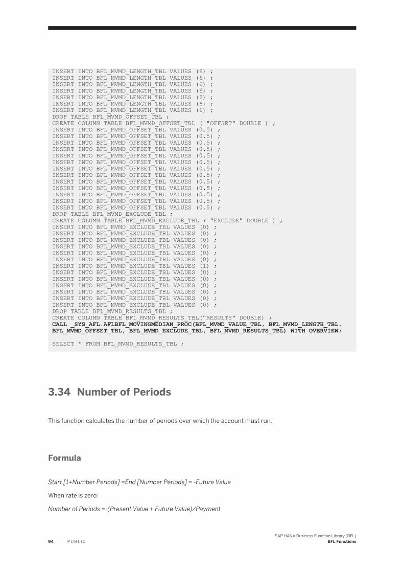
INSERT INTO BFL_MVMD_LENGTH_TBL VALUES (6) ;INSERT INTO BFL_MVMD_LENGTH_TBL VALUES (6) ;INSERT INTO BFL_MVMD_LENGTH_TBL VALUES (6) ;INSERT INTO BFL_MVMD_LENGTH_TBL VALUES (6) ;INSERT INTO BFL_MVMD_LENGTH_TBL VALUES (6) ;INSERT INTO BFL_MVMD_LENGTH_TBL VALUES (6) ;INSERT INTO BFL_MVMD_LENGTH_TBL VALUES (6) ;DROP TABLE BFL_MVMD_OFFSET_TBL ;CREATE COLUMN TABLE BFL_MVMD_OFFSET_TBL ( "OFFSET" DOUBLE ) ;INSERT INTO BFL_MVMD_OFFSET_TBL VALUES (0.5) ;INSERT INTO BFL_MVMD_OFFSET_TBL VALUES (0.5) ;INSERT INTO BFL_MVMD_OFFSET_TBL VALUES (0.5) ;INSERT INTO BFL_MVMD_OFFSET_TBL VALUES (0.5) ;INSERT INTO BFL_MVMD_OFFSET_TBL VALUES (0.5) ;INSERT INTO BFL_MVMD_OFFSET_TBL VALUES (0.5) ;INSERT INTO BFL_MVMD_OFFSET_TBL VALUES (0.5) ;INSERT INTO BFL_MVMD_OFFSET_TBL VALUES (0.5) ;INSERT INTO BFL_MVMD_OFFSET_TBL VALUES (0.5) ;INSERT INTO BFL_MVMD_OFFSET_TBL VALUES (0.5) ;INSERT INTO BFL_MVMD_OFFSET_TBL VALUES (0.5) ;INSERT INTO BFL_MVMD_OFFSET_TBL VALUES (0.5) ;INSERT INTO BFL_MVMD_OFFSET_TBL VALUES (0.5) ;DROP TABLE BFL_MVMD_EXCLUDE_TBL ;CREATE COLUMN TABLE BFL_MVMD_EXCLUDE_TBL ( "EXCLUDE" DOUBLE ) ;INSERT INTO BFL_MVMD_EXCLUDE_TBL VALUES (0) ;INSERT INTO BFL_MVMD_EXCLUDE_TBL VALUES (0) ;INSERT INTO BFL_MVMD_EXCLUDE_TBL VALUES (0) ;INSERT INTO BFL_MVMD_EXCLUDE_TBL VALUES (0) ;INSERT INTO BFL_MVMD_EXCLUDE_TBL VALUES (0) ;INSERT INTO BFL_MVMD_EXCLUDE_TBL VALUES (0) ;INSERT INTO BFL_MVMD_EXCLUDE_TBL VALUES (1) ;INSERT INTO BFL_MVMD_EXCLUDE_TBL VALUES (0) ;INSERT INTO BFL_MVMD_EXCLUDE_TBL VALUES (0) ;INSERT INTO BFL_MVMD_EXCLUDE_TBL VALUES (0) ;INSERT INTO BFL_MVMD_EXCLUDE_TBL VALUES (0) ;INSERT INTO BFL_MVMD_EXCLUDE_TBL VALUES (0) ;INSERT INTO BFL_MVMD_EXCLUDE_TBL VALUES (0) ;DROP TABLE BFL_MVMD_RESULTS_TBL ;CREATE COLUMN TABLE BFL_MVMD_RESULTS_TBL("RESULTS" DOUBLE) ; CALL _SYS_AFL.AFLBFL_MOVINGMEDIAN_PROC(BFL_MVMD_VALUE_TBL, BFL_MVMD_LENGTH_TBL, BFL_MVMD_OFFSET_TBL, BFL_MVMD_EXCLUDE_TBL, BFL_MVMD_RESULTS_TBL) WITH OVERVIEW; SELECT * FROM BFL_MVMD_RESULTS_TBL ;
3.34 Number of Periods
This function calculates the number of periods over which the account must run.
Formula
Start [1+Number Periods] =End [Number Periods] = -Future Value
When rate is zero:
Number of Periods =-(Present Value + Future Value)/Payment
94 P U B L I CSAP HANA Business Function Library (BFL)
BFL Functions

When rate is not zero:
Where:
Rate = {%rate}/100
and
Inter = (1+type*rate)*Payment/rate
Signature
Input Tables
Table 81:
Name Direction Number of Columns
Column Type Column Name Description
Rate Input Table 1 Double VALUE Rate percentage.
Present Input Table 1 Double VALUE The constant payment applied to the account each period.
Payment Input Table 1 Double VALUE The constant payment applied to the account each period.
Future Input Table 1 Double VALUE The value of the account at the end of the calculation.
Method Input Table 1 Double VALUE Specifies whether the payment is applied at the beginning or end of the period: ■ 0 = at the end of the period ■ 1 = at the beginning of the period
Output Table
SAP HANA Business Function Library (BFL)BFL Functions P U B L I C 95
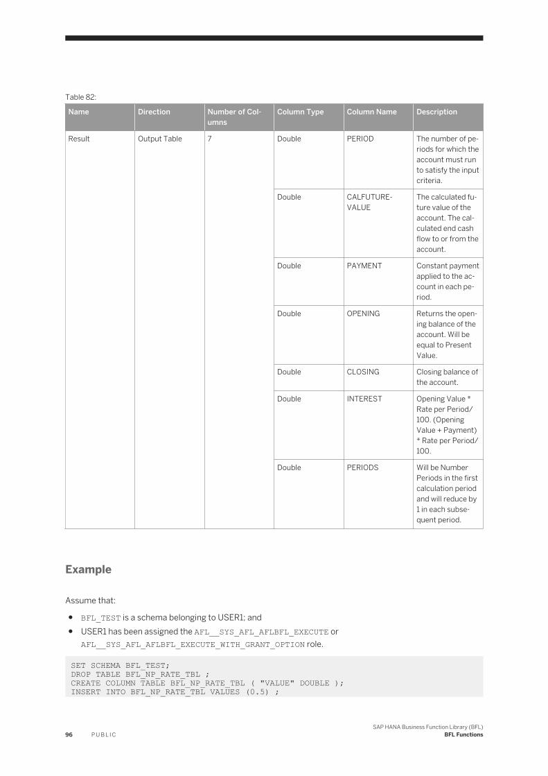
Table 82:
Name Direction Number of Columns
Column Type Column Name Description
Result Output Table 7 Double PERIOD The number of periods for which the account must run to satisfy the input criteria.
Double CALFUTUREVALUE
The calculated future value of the account. The calculated end cash flow to or from the account.
Double PAYMENT Constant payment applied to the account in each period.
Double OPENING Returns the opening balance of the account. Will be equal to Present Value.
Double CLOSING Closing balance of the account.
Double INTEREST Opening Value * Rate per Period/100. (Opening Value + Payment) * Rate per Period/100.
Double PERIODS Will be Number Periods in the first calculation period and will reduce by 1 in each subsequent period.
Example
Assume that:
● BFL_TEST is a schema belonging to USER1; and● USER1 has been assigned the AFL__SYS_AFL_AFLBFL_EXECUTE or
AFL__SYS_AFL_AFLBFL_EXECUTE_WITH_GRANT_OPTION role.
SET SCHEMA BFL_TEST; DROP TABLE BFL_NP_RATE_TBL ;CREATE COLUMN TABLE BFL_NP_RATE_TBL ( "VALUE" DOUBLE );INSERT INTO BFL_NP_RATE_TBL VALUES (0.5) ;
96 P U B L I CSAP HANA Business Function Library (BFL)
BFL Functions

INSERT INTO BFL_NP_RATE_TBL VALUES (0.5) ;DROP TABLE BFL_NP_PRESENT_TBL ;CREATE COLUMN TABLE BFL_NP_PRESENT_TBL ( "VALUE" DOUBLE ) ;INSERT INTO BFL_NP_PRESENT_TBL VALUES (10000) ;INSERT INTO BFL_NP_PRESENT_TBL VALUES (-10000) ;DROP TABLE BFL_NP_PAYMENT_TBL ;CREATE COLUMN TABLE BFL_NP_PAYMENT_TBL ( "VALUE" DOUBLE ) ;INSERT INTO BFL_NP_PAYMENT_TBL VALUES (500) ;INSERT INTO BFL_NP_PAYMENT_TBL VALUES (2500) ;DROP TABLE BFL_NP_FUTURE_TBL ;CREATE COLUMN TABLE BFL_NP_FUTURE_TBL ( "VALUE" DOUBLE ) ;INSERT INTO BFL_NP_FUTURE_TBL VALUES (12000) ;INSERT INTO BFL_NP_FUTURE_TBL VALUES (-2600) ;DROP TABLE BFL_NP_METHOD_TBL ;CREATE COLUMN TABLE BFL_NP_METHOD_TBL ( "VALUE" DOUBLE ) ;INSERT INTO BFL_NP_METHOD_TBL VALUES (1) ;INSERT INTO BFL_NP_METHOD_TBL VALUES (1) ;DROP TABLE BFL_NP_PERIODS_TBL ; CREATE COLUMN TABLE BFL_NP_PERIODS_TBL ( "PERIOD" DOUBLE,"CALFUTUREVALUE" DOUBLE,"PAYMENT" DOUBLE,"OPENING" DOUBLE, "CLOSING" DOUBLE,"INTEREST" DOUBLE, "PERIODS" DOUBLE); CALL _SYS_AFL.AFLBFL_NUMBERPERIODS_PROC(BFL_NP_RATE_TBL, BFL_NP_PRESENT_TBL, BFL_NP_PAYMENT_TBL, BFL_NP_FUTURE_TBL, BFL_NP_METHOD_TBL, BFL_NP_PERIODS_TBL) WITH OVERVIEW; SELECT * FROM BFL_NP_PERIODS_TBL ;
3.35 Net Present Value
This function calculates the net present value of a series of future cash flow. The result is the summation of the present values which are discounted based on the annual rate.
NPV always calculates for future periods and ignore the past data.
No restrictions are applied to:
1. The number of future payment2. The period between each payment does not need to be equal.
Formula
Where:
Pi is the Payment Value in the ith period.
di is the ith or last payment date.
SAP HANA Business Function Library (BFL)BFL Functions P U B L I C 97

dj is the date at which the Net Present Value is being calculated so that di - dj means the number of days forward from the day where Net Present Value is being calculated.
Rate is the discount rate per annum to apply to values in future periods.
Signature
Input Tables
Table 83:
Name Direction Number of Columns
Column Type Column Name Description
Rate Input Table 1 Double VALUE The annual rate at which future values are to be discounted.
Values Input Table 1 Double VALUE The series of cash values to be calculated.
Date Flag Input Table 1 Double VALUE Start(1); Mid(2); End(3); User(4)
Payment Date Input Table 1 String VALUE Date of Payment.
Days Input Table 1 Double VALUE Number of days in each period.
Output Table
Table 84:
Name Direction Number of Columns
Column Type Column Name Description
Result Output Table 1 Double NETPRESENTVALUE
The net present value of the series of cash flow.
Example
Assume that:
● BFL_TEST is a schema belonging to USER1; and● USER1 has been assigned the AFL__SYS_AFL_AFLBFL_EXECUTE or
AFL__SYS_AFL_AFLBFL_EXECUTE_WITH_GRANT_OPTION role.
SET SCHEMA BFL_TEST; DROP TABLE BFL_NPV_RATE_TBL;CREATE COLUMN TABLE BFL_NPV_RATE_TBL( "VALUE" DOUBLE );INSERT INTO BFL_NPV_RATE_TBL VALUES (0.05);INSERT INTO BFL_NPV_RATE_TBL VALUES (0.05);
98 P U B L I CSAP HANA Business Function Library (BFL)
BFL Functions

INSERT INTO BFL_NPV_RATE_TBL VALUES (0.05);INSERT INTO BFL_NPV_RATE_TBL VALUES (0.05);INSERT INTO BFL_NPV_RATE_TBL VALUES (0.05);INSERT INTO BFL_NPV_RATE_TBL VALUES (0.05);DROP TABLE BFL_NPV_VALUES_TBL;CREATE COLUMN TABLE BFL_NPV_VALUES_TBL( "VALUE" DOUBLE );INSERT INTO BFL_NPV_VALUES_TBL VALUES (-100000);INSERT INTO BFL_NPV_VALUES_TBL VALUES (60000);INSERT INTO BFL_NPV_VALUES_TBL VALUES (0);INSERT INTO BFL_NPV_VALUES_TBL VALUES (40000);INSERT INTO BFL_NPV_VALUES_TBL VALUES (50000);INSERT INTO BFL_NPV_VALUES_TBL VALUES (10000);DROP TABLE BFL_NPV_FLAG_TBL;CREATE COLUMN TABLE BFL_NPV_FLAG_TBL( "VALUE" INT );INSERT INTO BFL_NPV_FLAG_TBL VALUES (3);INSERT INTO BFL_NPV_FLAG_TBL VALUES (3);INSERT INTO BFL_NPV_FLAG_TBL VALUES (3);INSERT INTO BFL_NPV_FLAG_TBL VALUES (3);INSERT INTO BFL_NPV_FLAG_TBL VALUES (3);INSERT INTO BFL_NPV_FLAG_TBL VALUES (3);DROP TABLE BFL_NPV_USERDATE_TBL;CREATE COLUMN TABLE BFL_NPV_USERDATE_TBL( "VALUE" VARCHAR(255) );INSERT INTO BFL_NPV_USERDATE_TBL VALUES ('12/10/00');DROP TABLE BFL_NPV_DAYS_TBL;CREATE COLUMN TABLE BFL_NPV_DAYS_TBL( "VALUE" INT );INSERT INTO BFL_NPV_DAYS_TBL VALUES (90);INSERT INTO BFL_NPV_DAYS_TBL VALUES (91);INSERT INTO BFL_NPV_DAYS_TBL VALUES (92);INSERT INTO BFL_NPV_DAYS_TBL VALUES (92);INSERT INTO BFL_NPV_DAYS_TBL VALUES (365);INSERT INTO BFL_NPV_DAYS_TBL VALUES (365);DROP TABLE BFL_NPV_RESULT_TBL;CREATE COLUMN TABLE BFL_NPV_RESULT_TBL( "NETPRESENTVALUE" DOUBLE); CALL _SYS_AFL.AFLBFL_NETPRESENTVALUE_PROC(BFL_NPV_RATE_TBL, BFL_NPV_VALUES_TBL, BFL_NPV_FLAG_TBL, BFL_NPV_USERDATE_TBL, BFL_NPV_DAYS_TBL, BFL_NPV_RESULT_TBL) WITH OVERVIEW; SELECT * FROM BFL_NPV_RESULT_TBL;
3.36 Outlook
The Outlook is calculated by using actuals of past months and plan figures of future months. This is a critical function both for current shortfalls and overachievement. For shortfall, it drives management attention to key drivers, while for overachievement it reflects the necessary changes to the supply chain to meet increased demand.
The switchover date is taken as the first future period. The outlook for future periods is derived by revising the plan. The method is based on keeping the target for each subtotal the same as the plan, taking into account the actuals to date. In periods on/prior to switchover date, the outlook is calculated as equal to the actuals.
Formula
If the current period is before the period containing the switchover date, then:
Outlook = Actual
SAP HANA Business Function Library (BFL)BFL Functions P U B L I C 99
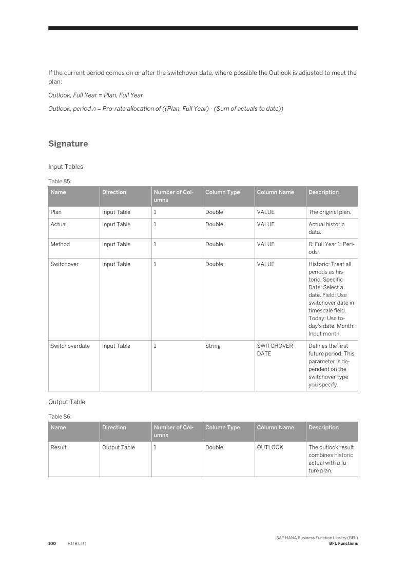
If the current period comes on or after the switchover date, where possible the Outlook is adjusted to meet the plan:
Outlook, Full Year = Plan, Full Year
Outlook, period n = Pro-rata allocation of ((Plan, Full Year) - (Sum of actuals to date))
Signature
Input Tables
Table 85:
Name Direction Number of Columns
Column Type Column Name Description
Plan Input Table 1 Double VALUE The original plan.
Actual Input Table 1 Double VALUE Actual historic data.
Method Input Table 1 Double VALUE 0: Full Year 1: Periods
Switchover Input Table 1 Double VALUE Historic: Treat all periods as historic. Specific Date: Select a date. Field: Use switchover date in timescale field. Today: Use today's date. Month: Input month.
Switchoverdate Input Table 1 String SWITCHOVERDATE
Defines the first future period. This parameter is dependent on the switchover type you specify.
Output Table
Table 86:
Name Direction Number of Columns
Column Type Column Name Description
Result Output Table 1 Double OUTLOOK The outlook result combines historic actual with a future plan.
100 P U B L I CSAP HANA Business Function Library (BFL)
BFL Functions

Example
Assume that:
● BFL_TEST is a schema belonging to USER1; and● USER1 has been assigned the AFL__SYS_AFL_AFLBFL_EXECUTE or
AFL__SYS_AFL_AFLBFL_EXECUTE_WITH_GRANT_OPTION role.
SET SCHEMA BFL_TEST; DROP TABLE BFL_OUTLOOK_PLAN_TBL ;CREATE COLUMN TABLE BFL_OUTLOOK_PLAN_TBL ( "VALUE" DOUBLE );INSERT INTO BFL_OUTLOOK_PLAN_TBL VALUES (1000) ;INSERT INTO BFL_OUTLOOK_PLAN_TBL VALUES (1000) ;INSERT INTO BFL_OUTLOOK_PLAN_TBL VALUES (1000) ;INSERT INTO BFL_OUTLOOK_PLAN_TBL VALUES (1000) ;INSERT INTO BFL_OUTLOOK_PLAN_TBL VALUES (1000) ;INSERT INTO BFL_OUTLOOK_PLAN_TBL VALUES (1000) ;INSERT INTO BFL_OUTLOOK_PLAN_TBL VALUES (1000) ;INSERT INTO BFL_OUTLOOK_PLAN_TBL VALUES (1000) ;INSERT INTO BFL_OUTLOOK_PLAN_TBL VALUES (1000) ;INSERT INTO BFL_OUTLOOK_PLAN_TBL VALUES (1000) ;INSERT INTO BFL_OUTLOOK_PLAN_TBL VALUES (1000) ;INSERT INTO BFL_OUTLOOK_PLAN_TBL VALUES (1000) ;DROP TABLE BFL_OUTLOOK_ACTUAL_TBL ;CREATE COLUMN TABLE BFL_OUTLOOK_ACTUAL_TBL ("VALUE" DOUBLE) ;INSERT INTO BFL_OUTLOOK_ACTUAL_TBL VALUES (500) ;INSERT INTO BFL_OUTLOOK_ACTUAL_TBL VALUES (500) ;INSERT INTO BFL_OUTLOOK_ACTUAL_TBL VALUES (500) ;INSERT INTO BFL_OUTLOOK_ACTUAL_TBL VALUES (500) ;INSERT INTO BFL_OUTLOOK_ACTUAL_TBL VALUES (500) ;INSERT INTO BFL_OUTLOOK_ACTUAL_TBL VALUES (500) ;INSERT INTO BFL_OUTLOOK_ACTUAL_TBL VALUES (500) ;DROP TABLE BFL_OUTLOOK_METHOD_TBL ;CREATE COLUMN TABLE BFL_OUTLOOK_METHOD_TBL ("VALUE" DOUBLE) ;INSERT INTO BFL_OUTLOOK_METHOD_TBL VALUES (0) ;DROP TABLE BFL_OUTLOOK_SWITCHOVER ;CREATE COLUMN TABLE BFL_OUTLOOK_SWITCHOVER ("VALUE" DOUBLE) ;INSERT INTO BFL_OUTLOOK_SWITCHOVER VALUES (1) ;DROP TABLE BFL_OUTLOOK_SWITCHOVERDATE ;CREATE COLUMN TABLE BFL_OUTLOOK_SWITCHOVERDATE ("SWITCHOVERDATE" VARCHAR(255)) ;INSERT INTO BFL_OUTLOOK_SWITCHOVERDATE VALUES ('20050701') ;DROP TABLE BFL_OUTLOOK_RESULTS_TBL ;CREATE COLUMN TABLE BFL_OUTLOOK_RESULTS_TBL ("OUTLOOK" DOUBLE) ; CALL _SYS_AFL.AFLBFL_OUTLOOK_PROC(BFL_OUTLOOK_PLAN_TBL, BFL_OUTLOOK_ACTUAL_TBL, BFL_OUTLOOK_METHOD_TBL, BFL_OUTLOOK_SWITCHOVER, BFL_OUTLOOK_SWITCHOVERDATE, BFL_OUTLOOK_RESULTS_TBL) WITH OVERVIEW; SELECT * FROM BFL_OUTLOOK_RESULTS_TBL ;
3.37 Payment
This function calculates the regular payment to an account for each period.
SAP HANA Business Function Library (BFL)BFL Functions P U B L I C 101

Formula
Start [1+Number Periods] =End [Number Periods] = -Future Value
When rate is zero, then:
Payment=-(Present Value +Future Value)/Number Periods
When rate is not zero:
and
Q=(1+type*rate)*(NR-1)/rate
Signature
Input Tables
Table 87:
Name Direction Number of Columns
Column Type Column Name Description
Rate Input Table 1 Double VALUE Rate per period as a percentage.
Periods Input Table 1 Double VALUE The number of periods to be run.
Present Input Table 1 Double VALUE Payment to/from the account initiating the calculation (can be zero).
Future Input Table 1 Double VALUE The payment to or from the account at the end of the calculation, which would be zero if a loan repays completely.
102 P U B L I CSAP HANA Business Function Library (BFL)
BFL Functions

Name Direction Number of Columns
Column Type Column Name Description
Method Input Table 1 Double VALUE ■ End of Period (0) ■ Beginning of Period (1)
Output Table
Table 88:
Name Direction Number of Columns
Column Type Column Name Description
Result Output Table 5 Double PAYMENT Constant payment applied to the account in each period.
Double OPENING Returns the opening balance of the account. Will be equal to Present Value.
Double CLOSING Closing balance of the account.
Double INTEREST Opening Value * Rate per Period/100. (Opening Value + Payment) * Rate per Period/100.
Double PERIODS Number Periods in the first calculation period and will reduce by 1 in each subsequent period.
Example
Assume that:
● BFL_TEST is a schema belonging to USER1; and● USER1 has been assigned the AFL__SYS_AFL_AFLBFL_EXECUTE or
AFL__SYS_AFL_AFLBFL_EXECUTE_WITH_GRANT_OPTION role.
SET SCHEMA BFL_TEST; DROP TABLE BFL_PAYMENT_RATE_TBL ;CREATE COLUMN TABLE BFL_PAYMENT_RATE_TBL ( "VALUE" DOUBLE ) ;INSERT INTO BFL_PAYMENT_RATE_TBL VALUES (0.5) ;INSERT INTO BFL_PAYMENT_RATE_TBL VALUES (0.5) ;DROP TABLE BFL_PAYMENT_PERIODS_TBL ;
SAP HANA Business Function Library (BFL)BFL Functions P U B L I C 103

CREATE COLUMN TABLE BFL_PAYMENT_PERIODS_TBL ( "VALUE" DOUBLE ) ;INSERT INTO BFL_PAYMENT_PERIODS_TBL VALUES (4) ;INSERT INTO BFL_PAYMENT_PERIODS_TBL VALUES (3) ;DROP TABLE BFL_PAYMENT_PRESENT_TBL ;CREATE COLUMN TABLE BFL_PAYMENT_PRESENT_TBL ( "VALUE" DOUBLE ) ;INSERT INTO BFL_PAYMENT_PRESENT_TBL VALUES (10000) ;INSERT INTO BFL_PAYMENT_PRESENT_TBL VALUES (-10000) ;DROP TABLE BFL_PAYMENT_FUTURE_TBL ;CREATE COLUMN TABLE BFL_PAYMENT_FUTURE_TBL ( "VALUE" DOUBLE ) ;INSERT INTO BFL_PAYMENT_FUTURE_TBL VALUES (-12000) ;INSERT INTO BFL_PAYMENT_FUTURE_TBL VALUES (-2600) ;DROP TABLE BFL_PAYMENT_METHOD_TBL ;CREATE COLUMN TABLE BFL_PAYMENT_METHOD_TBL ( "VALUE" DOUBLE ) ;INSERT INTO BFL_PAYMENT_METHOD_TBL VALUES (1) ;INSERT INTO BFL_PAYMENT_METHOD_TBL VALUES (1) ;DROP TABLE BFL_PAYMENT_RESULTS_TBL ; CREATE COLUMN TABLE BFL_PAYMENT_RESULTS_TBL ( "PAYMENT" DOUBLE, "OPENING" DOUBLE, "CLOSING" DOUBLE,"INTEREST" DOUBLE, "PERIODS" DOUBLE) ; CALL _SYS_AFL.AFLBFL_PAYMENT_PROC(BFL_PAYMENT_RATE_TBL, BFL_PAYMENT_PERIODS_TBL, BFL_PAYMENT_PRESENT_TBL, BFL_PAYMENT_FUTURE_TBL, BFL_PAYMENT_METHOD_TBL, BFL_PAYMENT_RESULTS_TBL) WITH OVERVIEW; SELECT * FROM BFL_PAYMENT_RESULTS_TBL ;
3.38 Present Value
This function calculates opening value given target closing balance and various parameters by assuming:
● Equal consecutive periods● Constant interest rate compounded to the account at the end of each period● A constant payment amount each period
Payments can be calculated at either the start or the end of the period.
Formula
Start [1+Number Periods] =End [Number Periods] =-Future Value
If Rate = 0, then:
Present Value = (Payment * Number Periods) + Future Value
If the rate is non-zero, then:
104 P U B L I CSAP HANA Business Function Library (BFL)
BFL Functions

Signature
Input Tables
Table 89:
Name Direction Number of Columns
Column Type Column Name Description
Rate Input Table 1 Double VALUE Rate per period.
Periods Input Table 1 Double VALUE The number of periods.
Payment Input Table 1 Double VALUE Constant payment applied each period.
Future Input Table 1 Double VALUE The payment to/from at the end of the calculation.
Method Input Table 1 Double VALUE ■ 0 = at the end of the period ■ 1 = at the beginning of the period
Output Table
Table 90:
Name Direction Number of Columns
Column Type Column Name Description
Result Output Table 6 Double ORIGINAL The start value or opening payment to or from the account in the first period.
Double PAYMENT Value of PAYMENT for every period
Double OPENING Opening balance of the account. Will be equal to Present Value.
Double CLOSING Closing balance of the account.
Double INTEREST Opening Value * Rate per Period/100. (Opening Value + Payment) * Rate per Period/100.
SAP HANA Business Function Library (BFL)BFL Functions P U B L I C 105

Name Direction Number of Columns
Column Type Column Name Description
Double PERIODS Will be Number Periods in the first calculation period and will reduce by 1 in each subsequent period.
Example
Assume that:
● BFL_TEST is a schema belonging to USER1; and● USER1 has been assigned the AFL__SYS_AFL_AFLBFL_EXECUTE or
AFL__SYS_AFL_AFLBFL_EXECUTE_WITH_GRANT_OPTION role.
SET SCHEMA BFL_TEST; DROP TABLE BFL_PV_RATE_TBL ; CREATE COLUMN TABLE BFL_PV_RATE_TBL ( "VALUE" DOUBLE ) ;INSERT INTO BFL_PV_RATE_TBL VALUES (0.5) ;INSERT INTO BFL_PV_RATE_TBL VALUES (0.5) ;DROP TABLE BFL_PV_PERIODS_TBL ;CREATE COLUMN TABLE BFL_PV_PERIODS_TBL ( "VALUE" DOUBLE ) ;INSERT INTO BFL_PV_PERIODS_TBL VALUES (4) ;INSERT INTO BFL_PV_PERIODS_TBL VALUES (3) ;DROP TABLE BFL_PV_PAYMENT_TBL ;CREATE COLUMN TABLE BFL_PV_PAYMENT_TBL ( "VALUE" DOUBLE ) ;INSERT INTO BFL_PV_PAYMENT_TBL VALUES (500) ;INSERT INTO BFL_PV_PAYMENT_TBL VALUES (2500) ;DROP TABLE BFL_PV_FUTURE_TBL ;CREATE COLUMN TABLE BFL_PV_FUTURE_TBL ( "VALUE" DOUBLE ) ;INSERT INTO BFL_PV_FUTURE_TBL VALUES (12000) ;INSERT INTO BFL_PV_FUTURE_TBL VALUES (-2600) ;DROP TABLE BFL_PV_METHOD_TBL ;CREATE COLUMN TABLE BFL_PV_METHOD_TBL ( "VALUE" DOUBLE ) ;INSERT INTO BFL_PV_METHOD_TBL VALUES (1) ;INSERT INTO BFL_PV_METHOD_TBL VALUES (1) ;DROP TABLE BFL_PV_PRESENT_TBL ; CREATE COLUMN TABLE BFL_PV_PRESENT_TBL ( "ORIGINAL" DOUBLE,"PAYMENT" DOUBLE,"OPENING" DOUBLE, "CLOSING" DOUBLE,"INTEREST" DOUBLE, "PERIODS" DOUBLE) ; CALL _SYS_AFL.AFLBFL_PRESENTVALUE_PROC(BFL_PV_RATE_TBL, BFL_PV_PERIODS_TBL, BFL_PV_PAYMENT_TBL, BFL_PV_FUTURE_TBL, BFL_PV_METHOD_TBL, BFL_PV_PRESENT_TBL) WITH OVERVIEW; SELECT * FROM BFL_PV_PRESENT_TBL ;
3.39 Proportion
This function allows you to input a start and end date, and then calculates the proportion of the period length.
106 P U B L I CSAP HANA Business Function Library (BFL)
BFL Functions

Formula
Proportion all days = (Stop date - Start date) / (Period finish date - Period start date)
Proportion working days is the same, but excludes weekends.
Signature
Input Tables
Table 91:
Name Direction Number of Columns
Column Type Column Name Description
Year Input Table 1 String VALUE The year to be calculated
Start Input Table 1 String VALUE Start Date
Stop Input Table 1 String VALUE End Date to be calculated
Output Table
Table 92:
Name Direction Number of Columns
Column Type Column Name Description
Result Output Table 1 Double PROPORTION The proportion of the period length
Example
Assume that:
● BFL_TEST is a schema belonging to USER1; and● USER1 has been assigned the AFL__SYS_AFL_AFLBFL_EXECUTE or
AFL__SYS_AFL_AFLBFL_EXECUTE_WITH_GRANT_OPTION role.
SET SCHEMA BFL_TEST; DROP TABLE BFL_PRPTN_YEAR_TBL ;CREATE COLUMN TABLE BFL_PRPTN_YEAR_TBL ( "VALUE" varchar(8) ) ;INSERT INTO BFL_PRPTN_YEAR_TBL VALUES ('2000');DROP TABLE BFL_PRPTN_START_TBL ;CREATE COLUMN TABLE BFL_PRPTN_START_TBL( "VALUE" varchar(8) );INSERT INTO BFL_PRPTN_START_TBL VALUES ('20000401');DROP TABLE BFL_PRPTN_STOP_TBL ;CREATE COLUMN TABLE BFL_PRPTN_STOP_TBL( "VALUE" varchar(8) );INSERT INTO BFL_PRPTN_STOP_TBL VALUES ('20000625');DROP TABLE BFL_PRPTN_RESULTS_TBL;CREATE COLUMN TABLE BFL_PRPTN_RESULTS_TBL ( "PROPORTION" DOUBLE) ; CALL _SYS_AFL.AFLBFL_PROPORTION_PROC(BFL_PRPTN_YEAR_TBL, BFL_PRPTN_START_TBL, BFL_PRPTN_STOP_TBL, BFL_PRPTN_RESULTS_TBL) WITH OVERVIEW;
SAP HANA Business Function Library (BFL)BFL Functions P U B L I C 107

SELECT * FROM BFL_PRPTN_RESULTS_TBL ;
3.40 Rate
This function helps to calculate the percentage interest rate of each period for an account. The four required inputs are start balance, end balance, payment per period and the number of periods. Because it is an iterative solution, more than one solution or no solution can be found for given inputs.
If Present Value, Future Value, and Payment are all input with the same sign then there will be no solution. If there is more than one solution, setting a non-zero value for parameter Estimate may cause an alternative rate value to be returned.
Assumptions:
● Equal consecutive periods● Constant, compounded interest rate applied at the end of each period● Payment is constant
Payment can be at the start or the end of the period.
Formula
Start [1+Number Periods] =End [Number Periods] = -Future Value
Rate is the solution to the family equation for the Payment, Present Value, Future Value, Number Periods, and Rate:
Rate is an iterative method requiring a start value. Therefore parameter Estimate is used as the starting value and is set to a default of 0.
Signature
Input Tables
108 P U B L I CSAP HANA Business Function Library (BFL)
BFL Functions

Table 93:
Name Direction Number of Columns
Column Type Column Name Description
Present Input Table 1 Double VALUE Value of the payment to/from the account at the beginning.
Periods Input Table 1 Double VALUE The number of periods the account runs.
Payment Input Table 1 Double VALUE Constant payment applied each period.
Future Input Table 1 Double VALUE The payment to/from at the end of the calculation.
Method Input Table 1 Double VALUE ■ 0 = at the end of the period ■ 1 = at the beginning of the period
Output Table
Table 94:
Name Direction Number of Columns
Column Type Column Name Description
Result Output Table 6 Double RATE The percentage rate per period for the account.
Double PAYMENT Value of PAYMENT for every period,
Double OPENING Opening balance of the account. Will be equal to Present Value,
Double CLOSING Closing balance of the account.
Double INTEREST Opening Value * Rate per Period/100. (Opening Value + Payment) * Rate per Period/100.
SAP HANA Business Function Library (BFL)BFL Functions P U B L I C 109

Name Direction Number of Columns
Column Type Column Name Description
Double PERIODS Will be Number Periods in the first calculation period and will reduce by 1 in each subsequent period.
Example
Assume that:
● BFL_TEST is a schema belonging to USER1; and● USER1 has been assigned the AFL__SYS_AFL_AFLBFL_EXECUTE or
AFL__SYS_AFL_AFLBFL_EXECUTE_WITH_GRANT_OPTION role.
SET SCHEMA BFL_TEST; DROP TABLE BFL_RATE_PRESENT_TBL ;CREATE COLUMN TABLE BFL_RATE_PRESENT_TBL ( "VALUE" DOUBLE ) ;INSERT INTO BFL_RATE_PRESENT_TBL VALUES (10000) ;INSERT INTO BFL_RATE_PRESENT_TBL VALUES (-10000) ;DROP TABLE BFL_RATE_PERIODS_TBL ;CREATE COLUMN TABLE BFL_RATE_PERIODS_TBL ( "VALUE" DOUBLE ) ;INSERT INTO BFL_RATE_PERIODS_TBL VALUES (4) ;INSERT INTO BFL_RATE_PERIODS_TBL VALUES (3) ;DROP TABLE BFL_RATE_PAYMENT_TBL ;CREATE COLUMN TABLE BFL_RATE_PAYMENT_TBL ( "VALUE" DOUBLE ) ;INSERT INTO BFL_RATE_PAYMENT_TBL VALUES (450) ;INSERT INTO BFL_RATE_PAYMENT_TBL VALUES (2500) ;DROP TABLE BFL_RATE_FUTURE_TBL ;CREATE COLUMN TABLE BFL_RATE_FUTURE_TBL ( "VALUE" DOUBLE ) ;INSERT INTO BFL_RATE_FUTURE_TBL VALUES (12000) ;INSERT INTO BFL_RATE_FUTURE_TBL VALUES (-2600) ;DROP TABLE BFL_RATE_METHOD_TBL ;CREATE COLUMN TABLE BFL_RATE_METHOD_TBL ( "VALUE" DOUBLE ) ;INSERT INTO BFL_RATE_METHOD_TBL VALUES (1) ;INSERT INTO BFL_RATE_METHOD_TBL VALUES (1) ;DROP TABLE BFL_RATE_RATE_TBL ; CREATE COLUMN TABLE BFL_RATE_RATE_TBL ( "RATE" DOUBLE, "PAYMENT" DOUBLE,"OPENING" DOUBLE, "CLOSING" DOUBLE,"INTEREST" DOUBLE, "PERIODS" DOUBLE); CALL _SYS_AFL.AFLBFL_RATE_PROC(BFL_RATE_PRESENT_TBL, BFL_RATE_PERIODS_TBL, BFL_RATE_PAYMENT_TBL, BFL_RATE_FUTURE_TBL, BFL_RATE_METHOD_TBL, BFL_RATE_RATE_TBL) WITH OVERVIEW; SELECT * FROM BFL_RATE_RATE_TBL ;
3.41 Repeat
This function repeats data of a single period or group of periods according to the time scale of the Dimension List.
110 P U B L I CSAP HANA Business Function Library (BFL)
BFL Functions
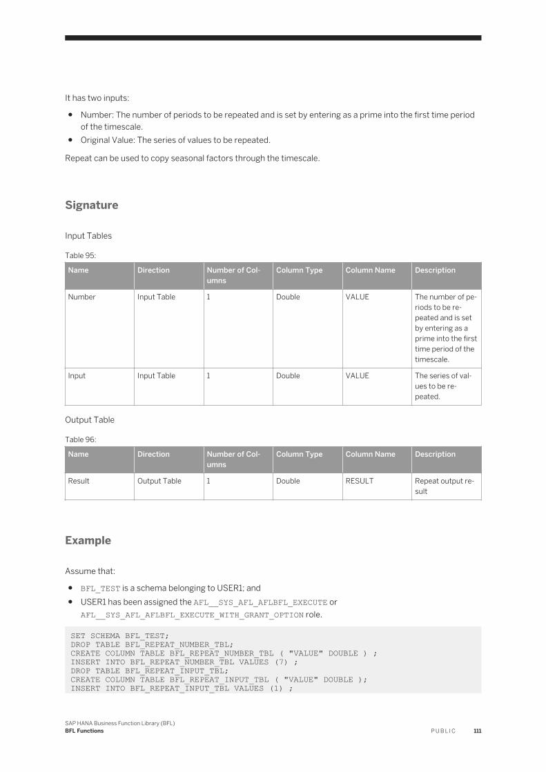
It has two inputs:
● Number: The number of periods to be repeated and is set by entering as a prime into the first time period of the timescale.
● Original Value: The series of values to be repeated.
Repeat can be used to copy seasonal factors through the timescale.
Signature
Input Tables
Table 95:
Name Direction Number of Columns
Column Type Column Name Description
Number Input Table 1 Double VALUE The number of periods to be repeated and is set by entering as a prime into the first time period of the timescale.
Input Input Table 1 Double VALUE The series of values to be repeated.
Output Table
Table 96:
Name Direction Number of Columns
Column Type Column Name Description
Result Output Table 1 Double RESULT Repeat output result
Example
Assume that:
● BFL_TEST is a schema belonging to USER1; and● USER1 has been assigned the AFL__SYS_AFL_AFLBFL_EXECUTE or
AFL__SYS_AFL_AFLBFL_EXECUTE_WITH_GRANT_OPTION role.
SET SCHEMA BFL_TEST; DROP TABLE BFL_REPEAT_NUMBER_TBL;CREATE COLUMN TABLE BFL_REPEAT_NUMBER_TBL ( "VALUE" DOUBLE ) ;INSERT INTO BFL_REPEAT_NUMBER_TBL VALUES (7) ;DROP TABLE BFL_REPEAT_INPUT_TBL; CREATE COLUMN TABLE BFL_REPEAT_INPUT_TBL ( "VALUE" DOUBLE );INSERT INTO BFL_REPEAT_INPUT_TBL VALUES (1) ;
SAP HANA Business Function Library (BFL)BFL Functions P U B L I C 111

INSERT INTO BFL_REPEAT_INPUT_TBL VALUES (1) ;INSERT INTO BFL_REPEAT_INPUT_TBL VALUES (1) ;INSERT INTO BFL_REPEAT_INPUT_TBL VALUES (1) ;INSERT INTO BFL_REPEAT_INPUT_TBL VALUES (1) ;INSERT INTO BFL_REPEAT_INPUT_TBL VALUES (0) ;INSERT INTO BFL_REPEAT_INPUT_TBL VALUES (0) ;DROP TABLE BFL_REPEAT_RESULTS_TBL; CREATE COLUMN TABLE BFL_REPEAT_RESULTS_TBL ( "RESULT" DOUBLE) ; CALL _SYS_AFL.AFLBFL_REPEAT_PROC(BFL_REPEAT_NUMBER_TBL, BFL_REPEAT_INPUT_TBL, BFL_REPEAT_RESULTS_TBL) WITH OVERVIEW; SELECT * FROM BFL_REPEAT_RESULTS_TBL ;
3.42 Rounding
This function calculates the rounded values for a specified input item according to a chosen rounding method. These rounding methods allow you to round figures up, down, away from zero (up for positive numbers, down for negative numbers), or toward zero (down for positive numbers, up for negative numbers).
You can combine the rounding methods with either of the below cumulative option:
1. Sum a series of rounded values2. Sum a series of non-rounded values and then rounding the total
Always, ensure the above two results are the same.
Signature
Input Tables
Table 97:
Name Direction Number of Columns
Column Type Column Name Description
Date Input Table 1 Double DATE The item with the values you want to round.
Precision Input Table 1 Double PRECISION The decimal interval. 1 = To nearest integer 0.1 = To 1 decimal place 0.01 = To 2 decimal places 1000 = To nearest 1000 0.25 = To nearest quarter 12 = To nearest dozen
112 P U B L I CSAP HANA Business Function Library (BFL)
BFL Functions

Name Direction Number of Columns
Column Type Column Name Description
Method Input Table 1 Double METHOD Nearest(0): Nearest rounds to the nearest whole integer. This is the default method. Up(1): Up rounds up to the nearest whole integer. Down(2): Down rounds down to the nearest whole integer. Away(3): Away from zero rounds a positive value up to the nearest whole integer and a negative value down to the nearest whole integer. Toward(4): Toward zero rounds a positive value down to the nearest whole integer and a negative value up to the nearest whole integer.
Output Table
Table 98:
Name Direction Number of Columns
Column Type Column Name Description
Result Output Table 1 Double ROUNDING The outlook result combines historic actual with a future plan.
Example
Assume that:
● BFL_TEST is a schema belonging to USER1; and● USER1 has been assigned the AFL__SYS_AFL_AFLBFL_EXECUTE or
AFL__SYS_AFL_AFLBFL_EXECUTE_WITH_GRANT_OPTION role.
SET SCHEMA BFL_TEST; DROP TABLE BFL_ROUND_DATE_TBL ;CREATE COLUMN TABLE BFL_ROUND_DATE_TBL ( "DATE" DOUBLE ) ;
SAP HANA Business Function Library (BFL)BFL Functions P U B L I C 113

INSERT INTO BFL_ROUND_DATE_TBL VALUES (200.1345);DROP TABLE BFL_ROUND_PRECISION_TBL ;CREATE COLUMN TABLE BFL_ROUND_PRECISION_TBL( "PRECISION" DOUBLE );INSERT INTO BFL_ROUND_PRECISION_TBL VALUES (0.1);DROP TABLE BFL_ROUND_METHOD_TBL ;CREATE COLUMN TABLE BFL_ROUND_METHOD_TBL( "METHOD" DOUBLE );INSERT INTO BFL_ROUND_METHOD_TBL VALUES (5);DROP TABLE BFL_ROUND_RESULTS_TBL;CREATE COLUMN TABLE BFL_ROUND_RESULTS_TBL ( "ROUNDING" DOUBLE) ; CALL _SYS_AFL.AFLBFL_ROUNDING_PROC(BFL_ROUND_DATE_TBL, BFL_ROUND_PRECISION_TBL, BFL_ROUND_METHOD_TBL, BFL_ROUND_RESULTS_TBL) WITH OVERVIEW; SELECT * FROM BFL_ROUND_RESULTS_TBL ;
3.43 Seasonal Simple&Seasonal Complex
These two built-in functions both perform seasonal adjustments of time to determine seasonal patterns in data. They use the same programs to calculate their results. They are different only in the number of methods and input and output variables available.
Seasonal Complex has more functionality and flexibility than Seasonal Simple and is intended for the highly advanced user of statistical data. Seasonal Simple is much easier to use because it uses fewer methods, inputs and outputs.
Method
The full Seasonal Complex model is following:
O=T*C*S*W*I
Where: O is the original data, T is the trend, C is the cyclical effect, S is the seasonal effect, I is the internal rate of return and W is working days.
Method 1- Basic method
1 = Multiplicative; 2 = Additive.
The multiplicative model is O = T * C * S * I. All Seasonal Simple methods are Multiplicative.
The arithmetic for additive model is O = T + C + S + I.
In the multiplicative model the seasonal effects add up to the number of periods in a year, whereas in an additive model they add up to zero.
For example, you must use Seasonal Complex if you want to expect the minimum temperature in a month to be better represented by an additive model, particularly if you want to compare the seasonal patterns of Year over Year Difference places.
Method 2- Average method
1 = Medial average; 2 = MA average; 3 = Average year; 4 = Typical year.
114 P U B L I CSAP HANA Business Function Library (BFL)
BFL Functions
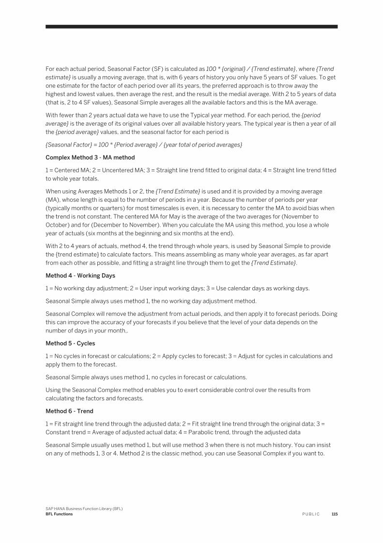
For each actual period, Seasonal Factor (SF) is calculated as 100 * {original} / {Trend estimate}, where {Trend estimate} is usually a moving average, that is, with 6 years of history you only have 5 years of SF values. To get one estimate for the factor of each period over all its years, the preferred approach is to throw away the highest and lowest values, then average the rest, and the result is the medial average. With 2 to 5 years of data (that is, 2 to 4 SF values), Seasonal Simple averages all the available factors and this is the MA average.
With fewer than 2 years actual data we have to use the Typical year method. For each period, the {period average} is the average of its original values over all available history years. The typical year is then a year of all the {period average} values, and the seasonal factor for each period is
{Seasonal Factor} = 100 * {Period average} / {year total of period averages}
Complex Method 3 - MA method
1 = Centered MA; 2 = Uncentered MA; 3 = Straight line trend fitted to original data; 4 = Straight line trend fitted to whole year totals.
When using Averages Methods 1 or 2, the {Trend Estimate} is used and it is provided by a moving average (MA), whose length is equal to the number of periods in a year. Because the number of periods per year (typically months or quarters) for most timescales is even, it is necessary to center the MA to avoid bias when the trend is not constant. The centered MA for May is the average of the two averages for (November to October) and for (December to November). When you calculate the MA using this method, you lose a whole year of actuals (six months at the beginning and six months at the end).
With 2 to 4 years of actuals, method 4, the trend through whole years, is used by Seasonal Simple to provide the {trend estimate} to calculate factors. This means assembling as many whole year averages, as far apart from each other as possible, and fitting a straight line through them to get the {Trend Estimate}.
Method 4 - Working Days
1 = No working day adjustment; 2 = User input working days; 3 = Use calendar days as working days.
Seasonal Simple always uses method 1, the no working day adjustment method.
Seasonal Complex will remove the adjustment from actual periods, and then apply it to forecast periods. Doing this can improve the accuracy of your forecasts if you believe that the level of your data depends on the number of days in your month,.
Method 5 - Cycles
1 = No cycles in forecast or calculations; 2 = Apply cycles to forecast; 3 = Adjust for cycles in calculations and apply them to the forecast.
Seasonal Simple always uses method 1, no cycles in forecast or calculations.
Using the Seasonal Complex method enables you to exert considerable control over the results from calculating the factors and forecasts.
Method 6 - Trend
1 = Fit straight line trend through the adjusted data; 2 = Fit straight line trend through the original data; 3 = Constant trend = Average of adjusted actual data; 4 = Parabolic trend, through the adjusted data
Seasonal Simple usually uses method 1, but will use method 3 when there is not much history. You can insist on any of methods 1, 3 or 4. Method 2 is the classic method, you can use Seasonal Complex if you want to.
SAP HANA Business Function Library (BFL)BFL Functions P U B L I C 115

3.43.1 Seasonal Complex
Formula
Seasonal Complex = Seasonal Complex (Method; ActFlag; Original; WorkingDays; Cycle%; OverFlag; OverValue; Factor; Adjusted; MovingAverage; Ratio; Trend; Cycle; Internal Rate of Returnegular; Calculated; Diagnostics)
Signature
Input Tables
Table 99:
Name Direction Number of Columns
Column Type Column Name Description
Original Input Table 1 Double ORIGINAL The data to be seasonally adjusted
Working Days Input Table 1 Double WORKINGDAYS The working days in the period
Cycle Input Table 1 Double CYCLE The cycle percent
Override Input Table 1 Double OVERRIDE Override flag
Override Value Input Table 1 Double OVERRIDEVALUE Override value
Config Input Table 1 Double CONFIG Has three rows, the meaning is as follows: Row 0: Specify method like in Seasonal Simple Row1: Specify the period number, refer to Seasonal Simple Row 2: Specify the forecast periods
Output Table
Table 100:
Name Direction Number of Columns
Column Type Column Name Description
Result Output Table 4 Double TREND The long term trend of the data
116 P U B L I CSAP HANA Business Function Library (BFL)
BFL Functions

Name Direction Number of Columns
Column Type Column Name Description
Double DIAGNOTICS A few simple diagnostics to evaluate the model
Double CALCULATED The forecast of the expected original value for every period
Double FORECAST OverValue if OverFlag = 1, Original if ActFlag = 1, otherwise Calculated
Example
Assume that:
● BFL_TEST is a schema belonging to USER1; and● USER1 has been assigned the AFL__SYS_AFL_AFLBFL_EXECUTE or
AFL__SYS_AFL_AFLBFL_EXECUTE_WITH_GRANT_OPTION role.
SET SCHEMA BFL_TEST; DROP TABLE BFL_SC_ORIGINAL_TBL ;CREATE COLUMN TABLE BFL_SC_ORIGINAL_TBL ( "ORIGINAL" DOUBLE ) ;INSERT INTO BFL_SC_ORIGINAL_TBL VALUES (150) ;INSERT INTO BFL_SC_ORIGINAL_TBL VALUES (108) ;INSERT INTO BFL_SC_ORIGINAL_TBL VALUES (112) ;INSERT INTO BFL_SC_ORIGINAL_TBL VALUES (115) ;INSERT INTO BFL_SC_ORIGINAL_TBL VALUES (119) ;INSERT INTO BFL_SC_ORIGINAL_TBL VALUES (115) ;INSERT INTO BFL_SC_ORIGINAL_TBL VALUES (115) ;INSERT INTO BFL_SC_ORIGINAL_TBL VALUES (115) ;INSERT INTO BFL_SC_ORIGINAL_TBL VALUES (134) ;INSERT INTO BFL_SC_ORIGINAL_TBL VALUES (139) ;INSERT INTO BFL_SC_ORIGINAL_TBL VALUES (143) ;INSERT INTO BFL_SC_ORIGINAL_TBL VALUES (240) ;INSERT INTO BFL_SC_ORIGINAL_TBL VALUES (220) ;INSERT INTO BFL_SC_ORIGINAL_TBL VALUES (155) ;INSERT INTO BFL_SC_ORIGINAL_TBL VALUES (162) ;INSERT INTO BFL_SC_ORIGINAL_TBL VALUES (166) ;INSERT INTO BFL_SC_ORIGINAL_TBL VALUES (172) ;INSERT INTO BFL_SC_ORIGINAL_TBL VALUES (170) ;INSERT INTO BFL_SC_ORIGINAL_TBL VALUES (171) ;INSERT INTO BFL_SC_ORIGINAL_TBL VALUES (169) ;INSERT INTO BFL_SC_ORIGINAL_TBL VALUES (188) ;INSERT INTO BFL_SC_ORIGINAL_TBL VALUES (195) ;INSERT INTO BFL_SC_ORIGINAL_TBL VALUES (198) ;INSERT INTO BFL_SC_ORIGINAL_TBL VALUES (320) ;INSERT INTO BFL_SC_ORIGINAL_TBL VALUES (300) ;INSERT INTO BFL_SC_ORIGINAL_TBL VALUES (220) ;INSERT INTO BFL_SC_ORIGINAL_TBL VALUES (222) ;DROP TABLE BFL_SC_WORKINGDAYS_TBL ;CREATE COLUMN TABLE BFL_SC_WORKINGDAYS_TBL ( "WORKINGDAYS" DOUBLE ) ;INSERT INTO BFL_SC_WORKINGDAYS_TBL VALUES (30) ;INSERT INTO BFL_SC_WORKINGDAYS_TBL VALUES (31) ;INSERT INTO BFL_SC_WORKINGDAYS_TBL VALUES (30) ;
SAP HANA Business Function Library (BFL)BFL Functions P U B L I C 117

INSERT INTO BFL_SC_WORKINGDAYS_TBL VALUES (30) ;INSERT INTO BFL_SC_WORKINGDAYS_TBL VALUES (30) ;INSERT INTO BFL_SC_WORKINGDAYS_TBL VALUES (31) ;INSERT INTO BFL_SC_WORKINGDAYS_TBL VALUES (30) ;INSERT INTO BFL_SC_WORKINGDAYS_TBL VALUES (30) ;INSERT INTO BFL_SC_WORKINGDAYS_TBL VALUES (30) ;INSERT INTO BFL_SC_WORKINGDAYS_TBL VALUES (28) ;INSERT INTO BFL_SC_WORKINGDAYS_TBL VALUES (30) ;INSERT INTO BFL_SC_WORKINGDAYS_TBL VALUES (30) ;INSERT INTO BFL_SC_WORKINGDAYS_TBL VALUES (29) ;INSERT INTO BFL_SC_WORKINGDAYS_TBL VALUES (30) ;INSERT INTO BFL_SC_WORKINGDAYS_TBL VALUES (31) ;INSERT INTO BFL_SC_WORKINGDAYS_TBL VALUES (31) ;INSERT INTO BFL_SC_WORKINGDAYS_TBL VALUES (31) ;INSERT INTO BFL_SC_WORKINGDAYS_TBL VALUES (30) ;INSERT INTO BFL_SC_WORKINGDAYS_TBL VALUES (30) ;INSERT INTO BFL_SC_WORKINGDAYS_TBL VALUES (30) ;INSERT INTO BFL_SC_WORKINGDAYS_TBL VALUES (29) ;INSERT INTO BFL_SC_WORKINGDAYS_TBL VALUES (30) ;INSERT INTO BFL_SC_WORKINGDAYS_TBL VALUES (30) ;INSERT INTO BFL_SC_WORKINGDAYS_TBL VALUES (30) ;INSERT INTO BFL_SC_WORKINGDAYS_TBL VALUES (30) ;INSERT INTO BFL_SC_WORKINGDAYS_TBL VALUES (29) ;INSERT INTO BFL_SC_WORKINGDAYS_TBL VALUES (30) ;INSERT INTO BFL_SC_WORKINGDAYS_TBL VALUES (31) ;DROP TABLE BFL_SC_CYCLE_TBL ;CREATE COLUMN TABLE BFL_SC_CYCLE_TBL ( "CYCLE" DOUBLE ) ;INSERT INTO BFL_SC_CYCLE_TBL VALUES (1) ;INSERT INTO BFL_SC_CYCLE_TBL VALUES (100) ;INSERT INTO BFL_SC_CYCLE_TBL VALUES (1) ;INSERT INTO BFL_SC_CYCLE_TBL VALUES (10) ;INSERT INTO BFL_SC_CYCLE_TBL VALUES (2002) ;DROP TABLE BFL_SC_OVERRIDE_TBL ;CREATE COLUMN TABLE BFL_SC_OVERRIDE_TBL("OVERRIDE" DOUBLE);INSERT INTO BFL_SC_OVERRIDE_TBL VALUES (1.0) ;DROP TABLE BFL_SC_OVERRIDEVALUE_TBL ;CREATE COLUMN TABLE BFL_SC_OVERRIDEVALUE_TBL("OVERRIDEVALUE" DOUBLE);INSERT INTO BFL_SC_OVERRIDEVALUE_TBL VALUES (10.0);DROP TABLE BFL_SC_CONFIG_TBL ;CREATE COLUMN TABLE BFL_SC_CONFIG_TBL("CONFIG" DOUBLE);INSERT INTO BFL_SC_CONFIG_TBL VALUES (111111);INSERT INTO BFL_SC_CONFIG_TBL VALUES (12);INSERT INTO BFL_SC_CONFIG_TBL VALUES (1);DROP TABLE BFL_SC_RESULTS_TBL ;CREATE COLUMN TABLE BFL_SC_RESULTS_TBL ("TREND" DOUBLE, "DIAGNOTICS" DOUBLE,"CALCULATED" DOUBLE, "FORECAST" DOUBLE) ; CALL _SYS_AFL.AFLBFL_SEASONALCOMPLEX_PROC(BFL_SC_ORIGINAL_TBL, BFL_SC_WORKINGDAYS_TBL, BFL_SC_CYCLE_TBL, BFL_SC_OVERRIDE_TBL, BFL_SC_OVERRIDEVALUE_TBL, BFL_SC_CONFIG_TBL, BFL_SC_RESULTS_TBL) WITH OVERVIEW; SELECT * FROM BFL_SC_RESULTS_TBL;
3.43.2 Seasonal Simple
Seasonal Simple is suitable for calculating data with sufficient history, at least one whole year, although five or more years are preferred and all trends are straight lines, and the data is of a multiplicative type. If you have a longer history and the seasonal factors have changed during the course of the history, other methods should be used.
118 P U B L I CSAP HANA Business Function Library (BFL)
BFL Functions

Formula
In Seasonal Simple the Cyclical and Working Day effects are not calculated, so the model is:
O = T * S * I
Seasonal Simple shows the seasonal factors as percentages (S = SF / 100) and replicates them throughout the time scale. The forecast is set equal to the historical value in the actual periods and calculated as T * SF / 100 for forecast periods.
Seasonal Simple has seven methods which use selected combinations of the six independent Seasonal Complex methods.
Table 101:
## Description Seasonal Complex Method Note
1 Based on the number of actuals: less than two complete years 2 or more, but less than 4 years 4 or more, but less than 6 years 6 or more years
141113 124111 121111 111111 1
2 Multiplicative, typical year, constant trend
141113 1, 2
3 Multiplicative, whole year initial trend, final trend through adjusted
124111 1, 3
4 Multiplicative, average, centered MA, trend through adjusted
121111 1, 4
5 Multiplicative, medial, centered MA, trend through adjusted
111111 1, 5
6 As method 1, but force constant trend
1xx113 1, 6
7 As method 1, but force linear trend
1xx111 1, 7
Note:
1. To choose the best Seasonal Simple method you must understand something of the Seasonal Complex methods, which are described above.
2. You can use this instead of method 1, even though you have more than 2 years of history.3. You can use this instead of method 1, even though you have more than 4 years of history.4. You can use this instead of method 1, even if you have 6 or more years of actuals.5. You can use this instead of method 1, even if you have less than 6 years of actuals.6. Use this method if you believe your data is most likely to stay constant, even though you have enough
actuals to get a good estimate of the slope.7. Use this method to use a linear trend, even though you have less than two years history.
SAP HANA Business Function Library (BFL)BFL Functions P U B L I C 119
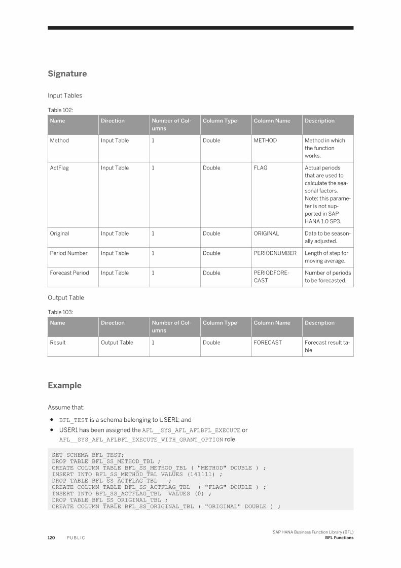
Signature
Input Tables
Table 102:
Name Direction Number of Columns
Column Type Column Name Description
Method Input Table 1 Double METHOD Method in which the function works.
ActFlag Input Table 1 Double FLAG Actual periods that are used to calculate the seasonal factors. Note: this parameter is not supported in SAP HANA 1.0 SP3.
Original Input Table 1 Double ORIGINAL Data to be seasonally adjusted.
Period Number Input Table 1 Double PERIODNUMBER Length of step for moving average.
Forecast Period Input Table 1 Double PERIODFORECAST
Number of periods to be forecasted.
Output Table
Table 103:
Name Direction Number of Columns
Column Type Column Name Description
Result Output Table 1 Double FORECAST Forecast result table
Example
Assume that:
● BFL_TEST is a schema belonging to USER1; and● USER1 has been assigned the AFL__SYS_AFL_AFLBFL_EXECUTE or
AFL__SYS_AFL_AFLBFL_EXECUTE_WITH_GRANT_OPTION role.
SET SCHEMA BFL_TEST; DROP TABLE BFL_SS_METHOD_TBL ;CREATE COLUMN TABLE BFL_SS_METHOD_TBL ( "METHOD" DOUBLE ) ;INSERT INTO BFL_SS_METHOD_TBL VALUES (141111) ;DROP TABLE BFL_SS_ACTFLAG_TBL ;CREATE COLUMN TABLE BFL_SS_ACTFLAG_TBL ( "FLAG" DOUBLE ) ;INSERT INTO BFL_SS_ACTFLAG_TBL VALUES (0) ;DROP TABLE BFL_SS_ORIGINAL_TBL ;CREATE COLUMN TABLE BFL_SS_ORIGINAL_TBL ( "ORIGINAL" DOUBLE ) ;
120 P U B L I CSAP HANA Business Function Library (BFL)
BFL Functions

INSERT INTO BFL_SS_ORIGINAL_TBL VALUES (150) ;INSERT INTO BFL_SS_ORIGINAL_TBL VALUES (108) ;INSERT INTO BFL_SS_ORIGINAL_TBL VALUES (112) ;INSERT INTO BFL_SS_ORIGINAL_TBL VALUES (115) ;INSERT INTO BFL_SS_ORIGINAL_TBL VALUES (119) ;INSERT INTO BFL_SS_ORIGINAL_TBL VALUES (115) ;INSERT INTO BFL_SS_ORIGINAL_TBL VALUES (115) ;INSERT INTO BFL_SS_ORIGINAL_TBL VALUES (115) ;INSERT INTO BFL_SS_ORIGINAL_TBL VALUES (134) ;INSERT INTO BFL_SS_ORIGINAL_TBL VALUES (139) ;INSERT INTO BFL_SS_ORIGINAL_TBL VALUES (143) ;INSERT INTO BFL_SS_ORIGINAL_TBL VALUES (240) ;INSERT INTO BFL_SS_ORIGINAL_TBL VALUES (220) ;INSERT INTO BFL_SS_ORIGINAL_TBL VALUES (155) ;INSERT INTO BFL_SS_ORIGINAL_TBL VALUES (162) ;INSERT INTO BFL_SS_ORIGINAL_TBL VALUES (166) ;INSERT INTO BFL_SS_ORIGINAL_TBL VALUES (172) ;INSERT INTO BFL_SS_ORIGINAL_TBL VALUES (170) ;INSERT INTO BFL_SS_ORIGINAL_TBL VALUES (171) ;INSERT INTO BFL_SS_ORIGINAL_TBL VALUES (169) ;INSERT INTO BFL_SS_ORIGINAL_TBL VALUES (188) ;INSERT INTO BFL_SS_ORIGINAL_TBL VALUES (195) ;INSERT INTO BFL_SS_ORIGINAL_TBL VALUES (198) ;INSERT INTO BFL_SS_ORIGINAL_TBL VALUES (320) ;INSERT INTO BFL_SS_ORIGINAL_TBL VALUES (300) ;INSERT INTO BFL_SS_ORIGINAL_TBL VALUES (220) ;INSERT INTO BFL_SS_ORIGINAL_TBL VALUES (222) ;DROP TABLE BFL_SS_PERIODNUMBER_TBL ;CREATE COLUMN TABLE BFL_SS_PERIODNUMBER_TBL("PERIODNUMBER" DOUBLE);INSERT INTO BFL_SS_PERIODNUMBER_TBL VALUES (12) ;DROP TABLE BFL_SS_FORECATPERIOD_TBL ;CREATE COLUMN TABLE BFL_SS_FORECATPERIOD_TBL("PERIODFORECAST" DOUBLE);INSERT INTO BFL_SS_FORECATPERIOD_TBL VALUES (1);DROP TABLE BFL_SS_FORECAST_TBL ;CREATE COLUMN TABLE BFL_SS_FORECAST_TBL ("FORECAST" DOUBLE) ; CALL _SYS_AFL.AFLBFL_SEASONALSIMPLE_PROC(BFL_SS_METHOD_TBL, BFL_SS_ACTFLAG_TBL, BFL_SS_ORIGINAL_TBL, BFL_SS_PERIODNUMBER_TBL, BFL_SS_FORECATPERIOD_TBL, BFL_SS_FORECAST_TBL) WITH OVERVIEW; SELECT * FROM BFL_SS_FORECAST_TBL;
3.44 Seasonal Simulation
This built-in function is used to test and explore how Seasonal Complex and other Business Functions handle the input data. It provides the building blocks to Seasonal Simulation seasonal data using a variety of characteristics.
Signature
Input Tables
SAP HANA Business Function Library (BFL)BFL Functions P U B L I C 121

Table 104:
Name Direction Number of Columns
Column Type Column Name Description
Method Input Table 1 Double METHOD Period(0) Repeat(1) Seasonal(2) BoxMuller(3) Random(4) Normal(5) Uniform(6) Repeated(7)
Periods Input Table 1 Double PERIODS Specify the period number
Param Input Table 1 Double PARAM Varies with the method data entered across the periods of the timescale as described below
Output Table
Table 105:
Name Direction Number of Columns
Column Type Column Name Description
Result Output Table 1 Double RESULT Seasonal simulation for time series
Example
Assume that:
● BFL_TEST is a schema belonging to USER1; and● USER1 has been assigned the AFL__SYS_AFL_AFLBFL_EXECUTE or
AFL__SYS_AFL_AFLBFL_EXECUTE_WITH_GRANT_OPTION role.
SET SCHEMA BFL_TEST; DROP TABLE BFL_SNSMLTN_METHOD_TBL;CREATE COLUMN TABLE BFL_SNSMLTN_METHOD_TBL ( "METHOD" DOUBLE ) ;INSERT INTO BFL_SNSMLTN_METHOD_TBL VALUES (6) ;DROP TABLE BFL_SNSMLTN_PERIODS_TBL; CREATE COLUMN TABLE BFL_SNSMLTN_PERIODS_TBL ( "PERIODS" DOUBLE ) ;INSERT INTO BFL_SNSMLTN_PERIODS_TBL VALUES (5) ;INSERT INTO BFL_SNSMLTN_PERIODS_TBL VALUES (5) ;DROP TABLE BFL_SNSMLTN_PARAM_TBL;CREATE COLUMN TABLE BFL_SNSMLTN_PARAM_TBL ( "PARAM" DOUBLE ) ;INSERT INTO BFL_SNSMLTN_PARAM_TBL VALUES (5.0) ;INSERT INTO BFL_SNSMLTN_PARAM_TBL VALUES (6.0) ;INSERT INTO BFL_SNSMLTN_PARAM_TBL VALUES (12.0) ;DROP TABLE BFL_SNSMLTN_RESULT_TBL; CREATE COLUMN TABLE BFL_SNSMLTN_RESULT_TBL ( "RESULT" DOUBLE) ; CALL _SYS_AFL.AFLBFL_SEASONALSIMULATION_PROC(BFL_SNSMLTN_METHOD_TBL, BFL_SNSMLTN_PERIODS_TBL, BFL_SNSMLTN_PARAM_TBL, BFL_SNSMLTN_RESULT_TBL) WITH OVERVIEW;
122 P U B L I CSAP HANA Business Function Library (BFL)
BFL Functions

SELECT * FROM BFL_SNSMLTN_RESULT_TBL;
3.45 Stock Flow
The Stock Flow figures out the level of supply needed in order to meet the prediction for stock cover.
Supply Outlook = Stock Flow(Prime;{Opening Stock};{Forecast Sales};{Forecast Cover};{Closing Stock};{Actual Sales};{Actual Cover};{Actual Supply};{Actual Closing};19980301;1;{Period Length};{Max Supply};{Min Supply};{% Wastage}; Wastage;0;1;1;{Sales Outlook})
The supply is calculated to meet the Closing Stock target.
Outlook method
Outlook Method determines how Sales Outlook is calculated.
Both Outlook methods try to set Sales Outlook to equal Actual Sales for historical periods and Forecast Sales for future periods. The default Outlook Method is Year over Year Difference. It allows for the Closing Stock to go negative in certain cases, identifying stock shortfalls. By setting the Outlook Method parameter to Restrict, parameters also can prevent Closing Stock from dropping below zero.
End Method
By default the demand in the last period is replicated, the last period sales are replicated to provide for future periods. Lengths of Period are replicated in a similar manner.
End Method can alternatively calculate an average demand over the last n periods and replicate this average over the future periods.
Min and Max Supply
The maximum supply can be restricted due to warehouse capacity, existing contracts, production constraints...etc. Minimum supply can be restricted where stock can only be depleted at the rate of sales. For example, in June there is an actual stock cover of over 80 days but only a planned cover of 30 days for July. Even with zero incoming supply, sales in June will not reduce stock levels to the planned levels. This then requires disposal (or donation) of stock to bring the stock levels down quickly. The closing stock levels and actual stock cover are adjusted accordingly.
Wastage
Wastage for each period to cover a variety of non-sales related stock reduction, such as shrinkage, spoilage, etc.
Cover Units and Period Length
Based on the Sales Outlook, using calendar days, Cover Units Forecast Cover is measured in stock-turn days.
Rounding Method
By default, there is no rounding of discrete units. You can use the rounding method to round each element or to round each time total (preserve sum and preserve sum YoY ). Using the preserve sum methods, the elements are rounded in such a way that they continue to add up to the time total.
SAP HANA Business Function Library (BFL)BFL Functions P U B L I C 123

Signature
Input Tables
Table 106:
Name Direction Number of Columns
Column Type Column Name Description
Prime Input Table 1 Double PRIME Prime - opening stock of the first period.
Time Input Table 1 String TIME The calculated time.
Forecast Sales Input Table 1 Double FORECASTSALES Forecast sales will be used in the period containing the switchover date and there after. Prior to the switchover date there is no forecast, only actuals.
Forecast Cover Input Table 1 Double FORECASTCOVER The forecast stock cover. How many days/periods of future sales the closing stock should support. 100 means to set Closing Stock at such a level that it lasts 100 days based on Sales Outlook.
Actual Sales Input Table 1 Double ACTUALSALES Actual sales input for historic periods only.
Actual Supply Input Table 1 Double ACTUALSUPPLY Actual supply input for historic periods only.
Actual Closing Input Table 1 Double ACTUALCLOSING Actual closing stock input for historic periods only.
Switchover Input Table 1 Int SWITCHOVER The period containing the switchover date is defined as the first future period.
124 P U B L I CSAP HANA Business Function Library (BFL)
BFL Functions

Name Direction Number of Columns
Column Type Column Name Description
Switchover Date Input Table 1 String SWITCHOVERDATE
Specify the switchover date base on Switchover
Cover Units Input Table 1 Int COVERUNITS Identifies the measure for Stock Cover in terms of future sales. Days: Use calendar days. Default. Units: Use custom units from the item Period Length Periods: Use number of periods. Each detail item in the timescale field is a period.
Period Length Input Table 1 Int PERIODLENGTH Available if you want to use non-standard calendar period lengths. For example: 4 - 4 - 5 for weeks in each period. Period Length will be ignored unless you set Cover Units=Period.
Max Supply Input Table 1 Double MAXSUPPLY Physical limitations (constraints) to the maximum supply available to increase stock levels (warehouse space, etc). If left blank, the default is for Max Supply to be allowed to go to infinity.
Min Supply Input Table 1 Double MINSUPPLY Limitation to the flow out of stock.
SAP HANA Business Function Library (BFL)BFL Functions P U B L I C 125

Name Direction Number of Columns
Column Type Column Name Description
Wastage Rate Input Table 1 Double WASTAGERATE Changes in stock due to shrinkage (not explained by sales and supply). Wastage is = to % Wastage applied to the Opening Stock.
Rounding Method Input Table 1 Int ROUNDMETHOD DNR: Do not round. This is the default if left blank (no partial units…discrete). Round: Round each element (process). Preserve Sum: Preserve the sum by changing the most obvious element(s)….where rounded value is furthest from original value. Preserve Sum YoY: Preserve the sum by rounding cumulated data and then taking the Year over Year Difference (the default).
End Method Input Table 1 Int ENDMETHOD Integer Constant: The number of periods over which to average sales when projecting beyond the last period in the timescale. This is used in the closing stock calculation toward the end of the timescale. N periods: Use the average of the last 3 periods to project sales forward.
126 P U B L I CSAP HANA Business Function Library (BFL)
BFL Functions

Name Direction Number of Columns
Column Type Column Name Description
Outlook Method Input Table 1 Int OUTLOOKMETHOD
How Forecast Sales input is used to provide future Sales Outlook. Default: Use Forecast Sales from the period containing the switchover date onwards, Actual Sales prior to this (the default method). Restrict: Restrict future sales if closing stock goes negative.
Output Table
Table 107:
Name Direction Number of Columns
Column Type Column Name Description
Result Output Table 6 Double OPENING Opening Stock. Fed from the Closing Stock of the previous period.
Double CLOSING Closing Stock. Actual Closing Stock prior to the switchover date; the level required to meet the Forecast Stock Cover thereafter.
Double ACTUALCOVER Actual Stock Cover. How many days/periods of future sales the Closing Stock actually does support.
SAP HANA Business Function Library (BFL)BFL Functions P U B L I C 127

Name Direction Number of Columns
Column Type Column Name Description
Double WASTAGE Changes in stock due to shrinkage (not explained by sales and supply). Wastage is = to % Wastage applied to the Opening Stock.
Double SALESOUTLOOK Sales Outlook is equal to the Actual Sales history prior to the switchover date, Forecast Sales thereafter. See Outlook Method.
Double SUPPLYOUTLOOK The supply in future periods required to meet forecast stock cover based on forecast sales. The supply is subject to the constraints of Min and Max Supply. Prior to the switchover date, Supply Outlook equals Actual Supply.
Example
Assume that:
● BFL_TEST is a schema belonging to USER1; and● USER1 has been assigned the AFL__SYS_AFL_AFLBFL_EXECUTE or
AFL__SYS_AFL_AFLBFL_EXECUTE_WITH_GRANT_OPTION role.
SET SCHEMA BFL_TEST; DROP TABLE BFL_SF_PRIME_TBL;CREATE COLUMN TABLE BFL_SF_PRIME_TBL ("PRIME" DOUBLE);INSERT INTO BFL_SF_PRIME_TBL VALUES(10000);DROP TABLE BFL_SF_TIME_TBL;CREATE COLUMN TABLE BFL_SF_TIME_TBL ("TIME" VARCHAR(255));INSERT INTO BFL_SF_TIME_TBL VALUES('20100801');INSERT INTO BFL_SF_TIME_TBL VALUES('20100912');INSERT INTO BFL_SF_TIME_TBL VALUES('20101020');INSERT INTO BFL_SF_TIME_TBL VALUES('20101130');INSERT INTO BFL_SF_TIME_TBL VALUES('20110105');INSERT INTO BFL_SF_TIME_TBL VALUES('20110220');
128 P U B L I CSAP HANA Business Function Library (BFL)
BFL Functions

DROP TABLE BFL_SF_FORECASTSALES_TBL;CREATE COLUMN TABLE BFL_SF_FORECASTSALES_TBL ("FORECASTSALES" DOUBLE);INSERT INTO BFL_SF_FORECASTSALES_TBL VALUES(0);INSERT INTO BFL_SF_FORECASTSALES_TBL VALUES(0);INSERT INTO BFL_SF_FORECASTSALES_TBL VALUES(2500);INSERT INTO BFL_SF_FORECASTSALES_TBL VALUES(3000);INSERT INTO BFL_SF_FORECASTSALES_TBL VALUES(2500);INSERT INTO BFL_SF_FORECASTSALES_TBL VALUES(3500);DROP TABLE BFL_SF_FORECASTCOVER_TBL;CREATE COLUMN TABLE BFL_SF_FORECASTCOVER_TBL ("FORECASTCOVER" DOUBLE);INSERT INTO BFL_SF_FORECASTCOVER_TBL VALUES(0);INSERT INTO BFL_SF_FORECASTCOVER_TBL VALUES(0);INSERT INTO BFL_SF_FORECASTCOVER_TBL VALUES(100);INSERT INTO BFL_SF_FORECASTCOVER_TBL VALUES(70);INSERT INTO BFL_SF_FORECASTCOVER_TBL VALUES(75);INSERT INTO BFL_SF_FORECASTCOVER_TBL VALUES(50);DROP TABLE BFL_SF_ACTUALSALES_TBL;CREATE COLUMN TABLE BFL_SF_ACTUALSALES_TBL ("ACTUALSALES" DOUBLE);INSERT INTO BFL_SF_ACTUALSALES_TBL VALUES(1500);INSERT INTO BFL_SF_ACTUALSALES_TBL VALUES(2000);DROP TABLE BFL_SF_ACTUALSUPPLY_TBL;CREATE COLUMN TABLE BFL_SF_ACTUALSUPPLY_TBL ("ACTUALSUPPLY" DOUBLE);INSERT INTO BFL_SF_ACTUALSUPPLY_TBL VALUES(2000);INSERT INTO BFL_SF_ACTUALSUPPLY_TBL VALUES(2500);DROP TABLE BFL_SF_ACTUALCLOSING_TBL;CREATE COLUMN TABLE BFL_SF_ACTUALCLOSING_TBL ("ACTUALCLOSING" DOUBLE);INSERT INTO BFL_SF_ACTUALCLOSING_TBL VALUES(10000);INSERT INTO BFL_SF_ACTUALCLOSING_TBL VALUES(10000);DROP TABLE BFL_SF_SWITCHOVER_TBL;CREATE COLUMN TABLE BFL_SF_SWITCHOVER_TBL ("SWITCHOVER" INTEGER);INSERT INTO BFL_SF_SWITCHOVER_TBL VALUES(1);DROP TABLE BFL_SF_SWITCHOVERDATE_TBL;CREATE COLUMN TABLE BFL_SF_SWITCHOVERDATE_TBL ("SWITCHOVERDATE" VARCHAR(255));INSERT INTO BFL_SF_SWITCHOVERDATE_TBL VALUES('20101001');DROP TABLE BFL_SF_COVERUNITS_TBL;CREATE COLUMN TABLE BFL_SF_COVERUNITS_TBL ("COVERUNITS" INTEGER);INSERT INTO BFL_SF_COVERUNITS_TBL VALUES(0);DROP TABLE BFL_SF_PERIODLENGTH_TBL;CREATE COLUMN TABLE BFL_SF_PERIODLENGTH_TBL ("PERIODLENGTH" INTEGER);INSERT INTO BFL_SF_PERIODLENGTH_TBL VALUES(0);DROP TABLE BFL_SF_MAXSUPPLY_TBL;CREATE COLUMN TABLE BFL_SF_MAXSUPPLY_TBL ("MAXSUPPLY" DOUBLE);INSERT INTO BFL_SF_MAXSUPPLY_TBL VALUES(0);INSERT INTO BFL_SF_MAXSUPPLY_TBL VALUES(0);INSERT INTO BFL_SF_MAXSUPPLY_TBL VALUES(0);INSERT INTO BFL_SF_MAXSUPPLY_TBL VALUES(0);INSERT INTO BFL_SF_MAXSUPPLY_TBL VALUES(0);INSERT INTO BFL_SF_MAXSUPPLY_TBL VALUES(0);DROP TABLE BFL_SF_MINSUPPLY_TBL;CREATE COLUMN TABLE BFL_SF_MINSUPPLY_TBL ("MINSUPPLY" DOUBLE);INSERT INTO BFL_SF_MINSUPPLY_TBL VALUES(0);INSERT INTO BFL_SF_MINSUPPLY_TBL VALUES(0);INSERT INTO BFL_SF_MINSUPPLY_TBL VALUES(0);INSERT INTO BFL_SF_MINSUPPLY_TBL VALUES(0);INSERT INTO BFL_SF_MINSUPPLY_TBL VALUES(0);INSERT INTO BFL_SF_MINSUPPLY_TBL VALUES(0);DROP TABLE BFL_SF_WASTAGERATE_TBL;CREATE COLUMN TABLE BFL_SF_WASTAGERATE_TBL ("WASTAGERATE" DOUBLE);INSERT INTO BFL_SF_WASTAGERATE_TBL VALUES(5);INSERT INTO BFL_SF_WASTAGERATE_TBL VALUES(5);INSERT INTO BFL_SF_WASTAGERATE_TBL VALUES(5);INSERT INTO BFL_SF_WASTAGERATE_TBL VALUES(5);INSERT INTO BFL_SF_WASTAGERATE_TBL VALUES(5);INSERT INTO BFL_SF_WASTAGERATE_TBL VALUES(5);DROP TABLE BFL_SF_ROUNDMETHOD_TBL;CREATE COLUMN TABLE BFL_SF_ROUNDMETHOD_TBL ("ROUNDMETHOD" INTEGER);INSERT INTO BFL_SF_ROUNDMETHOD_TBL VALUES(0);DROP TABLE BFL_SF_ENDMETHOD_TBL;
SAP HANA Business Function Library (BFL)BFL Functions P U B L I C 129

CREATE COLUMN TABLE BFL_SF_ENDMETHOD_TBL ("ENDMETHOD" INTEGER);INSERT INTO BFL_SF_ENDMETHOD_TBL VALUES(2);DROP TABLE BFL_SF_OUTLOOKMETHOD_TBL;CREATE COLUMN TABLE BFL_SF_OUTLOOKMETHOD_TBL ("OUTLOOKMETHOD" INTEGER);INSERT INTO BFL_SF_OUTLOOKMETHOD_TBL VALUES(0);DROP TABLE BFL_SF_RESULTS_TBL;CREATE COLUMN TABLE BFL_SF_RESULTS_TBL ("OPENING" DOUBLE,"CLOSING" DOUBLE,"ACTUALCOVER" DOUBLE,"WASTAGE" DOUBLE,"SALESOUTLOOK" DOUBLE,"SUPPLYOUTLOOK" DOUBLE); CALL _SYS_AFL.AFLBFL_STOCKFLOW_PROC(BFL_SF_PRIME_TBL, BFL_SF_TIME_TBL, BFL_SF_FORECASTSALES_TBL, BFL_SF_FORECASTCOVER_TBL, BFL_SF_ACTUALSALES_TBL, BFL_SF_ACTUALSUPPLY_TBL, BFL_SF_ACTUALCLOSING_TBL, BFL_SF_SWITCHOVER_TBL, BFL_SF_SWITCHOVERDATE_TBL, BFL_SF_COVERUNITS_TBL, BFL_SF_PERIODLENGTH_TBL , BFL_SF_MAXSUPPLY_TBL, BFL_SF_MINSUPPLY_TBL, BFL_SF_WASTAGERATE_TBL, BFL_SF_ROUNDMETHOD_TBL, BFL_SF_ENDMETHOD_TBL, BFL_SF_OUTLOOKMETHOD_TBL, BFL_SF_RESULTS_TBL ) WITH OVERVIEW; SELECT * FROM BFL_SF_RESULTS_TBL;
3.46 Stock Flow Reverse
This function is based on the standard Stock Flow Business Function. In Stock Flow, the switchover date applies to the entire timescale, but in Stock Flow Reverse, an actual/forecast flag acts as a Year over Year Difference switchover date. This allows stock flow simulation for Year over Year Difference scenarios where the switchover date may vary due to departure from standard calendars and periods (projects).
Signature
Input Tables
Table 108:
Name Direction Number of Columns
Column Type Column Name Description
Prime Input Table 1 Double PRIME Prime - opening stock of the first period.
Time Input Table 1 String TIME The calculated time.
Forecast Sales Input Table 1 Double FORECASTSALES Forecast sales will be used in the period containing the switchover date and thereafter. Prior to the switchover date there is no forecast, only actual.
130 P U B L I CSAP HANA Business Function Library (BFL)
BFL Functions

Name Direction Number of Columns
Column Type Column Name Description
Forecast Cover Input Table 1 Double FORECASTCOVER The forecast stock cover. How many days/periods of future sales the closing stock should support. 100 sets Closing Stock at such a level that it lasts 100 days based on Sales Outlook.
Actual Sales Input Table 1 Double ACTUALSALES Actual Sales input for historic periods only.
Actual Supply Input Table 1 Double ACTUALSUPPLY Actual Supply input for historic periods only.
Actual Closing Input Table 1 Double ACTUALCLOSING Actual Closing Stock input for historic periods only.
Forecast Flag Input Table 1 Int FORECASTFLAG Enter a flag to set a Year over Year Difference switchover date on each page. The first value > 1 indicates the start of forecast periods.
Cover Units Input Table 1 Int COVERUNITS Identifies the measure for Stock Cover in terms of future sales. Days: Use calendar days. Default. Units: Use custom units from the item Period Length. Periods: Use number of periods. Each detail item in the timescale field is a period.
SAP HANA Business Function Library (BFL)BFL Functions P U B L I C 131
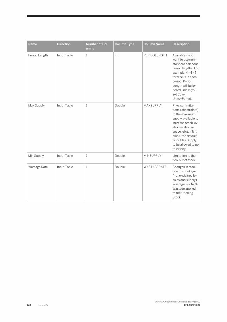
Name Direction Number of Columns
Column Type Column Name Description
Period Length Input Table 1 Int PERIODLENGTH Available if you want to use non-standard calendar period lengths. For example: 4 - 4 - 5 for weeks in each period. Period Length will be ignored unless you set Cover Units=Period.
Max Supply Input Table 1 Double MAXSUPPLY Physical limitations (constraints) to the maximum supply available to increase stock levels (warehouse space, etc). If left blank, the default is for Max Supply to be allowed to go to infinity.
Min Supply Input Table 1 Double MINSUPPLY Limitation to the flow out of stock.
Wastage Rate Input Table 1 Double WASTAGERATE Changes in stock due to shrinkage (not explained by sales and supply). Wastage is = to % Wastage applied to the Opening Stock.
132 P U B L I CSAP HANA Business Function Library (BFL)
BFL Functions

Name Direction Number of Columns
Column Type Column Name Description
Rounding Method Input Table 1 Int ROUNDMETHOD DNR: Do not round. This is the default if left blank (no partial units, that is discrete only). Round: Round each element (process). Preserve Sum: Preserve the sum by changing the most obvious element(s), where rounded value is furthest from original value. Preserve Sum YoY: Preserve the sum by rounding cumulated data and then taking the Year over Year Difference (the default).
End Method Input Table 1 Int ENDMETHOD Integer Constant: The number of periods over which to average sales when projecting beyond the last period in the timescale. This is used in the Closing Stock calculation toward the end of the timescale. N periods: Use the average of the last 3 periods to project sales forward.
SAP HANA Business Function Library (BFL)BFL Functions P U B L I C 133

Name Direction Number of Columns
Column Type Column Name Description
Outlook Method Input Table 1 Int OUTLOOKMETHOD
How forecast sales input is used to provide future sales outlook. Default: Use Forecast Sales from the period containing the switchover date onwards, Actual Sales prior to this (the default method). Restrict: Restrict future sales if closing stock goes negative.
Output Table
Table 109:
Name Direction Number of Columns
Column Type Column Name Description
Result Output Table 6 Double OPENING Opening Stock. Fed from the Closing Stock of the previous period.
Double CLOSING Closing Stock. Actual Closing Stock prior to the switchover date; the level required to meet the Forecast Stock Cover thereafter.
Double ACTUALCOVER Actual Stock Cover. How many days/periods of future sales the Closing Stock actually does support.
Double WASTAGE Changes in stock due to shrinkage (not explained by sales and supply). Wastage is = to % Wastage applied to the Opening Stock.
134 P U B L I CSAP HANA Business Function Library (BFL)
BFL Functions

Name Direction Number of Columns
Column Type Column Name Description
Double SALESOUTLOOK Sales Outlook is equal to the Actual Sales history prior to the switchover date, Forecast Sales thereafter. See Outlook Method.
Double SUPPLYOUTLOOK The supply in future periods required to meet forecast stock cover based on forecast sales. The supply is subject to the constraints of Min and Max Supply. Prior to the switchover date, Supply Outlook equals Actual Supply.
Example
Assume that:
● BFL_TEST is a schema belonging to USER1; and● USER1 has been assigned the AFL__SYS_AFL_AFLBFL_EXECUTE or
AFL__SYS_AFL_AFLBFL_EXECUTE_WITH_GRANT_OPTION role.
SET SCHEMA BFL_TEST; DROP TABLE BFL_SFR_PRIME_TBL;CREATE COLUMN TABLE BFL_SFR_PRIME_TBL ("PRIME" DOUBLE);INSERT INTO BFL_SFR_PRIME_TBL VALUES(10000);DROP TABLE BFL_SFR_TIME_TBL;CREATE COLUMN TABLE BFL_SFR_TIME_TBL ("TIME" VARCHAR(255));INSERT INTO BFL_SFR_TIME_TBL VALUES('20100801');INSERT INTO BFL_SFR_TIME_TBL VALUES('20100912');INSERT INTO BFL_SFR_TIME_TBL VALUES('20101020');INSERT INTO BFL_SFR_TIME_TBL VALUES('20101130');INSERT INTO BFL_SFR_TIME_TBL VALUES('20110105');INSERT INTO BFL_SFR_TIME_TBL VALUES('20110220');DROP TABLE BFL_SFR_FORECASTSALES_TBL;CREATE COLUMN TABLE BFL_SFR_FORECASTSALES_TBL ("FORECASTSALES" DOUBLE);INSERT INTO BFL_SFR_FORECASTSALES_TBL VALUES(0);INSERT INTO BFL_SFR_FORECASTSALES_TBL VALUES(0);INSERT INTO BFL_SFR_FORECASTSALES_TBL VALUES(2500);INSERT INTO BFL_SFR_FORECASTSALES_TBL VALUES(3000);INSERT INTO BFL_SFR_FORECASTSALES_TBL VALUES(2500);INSERT INTO BFL_SFR_FORECASTSALES_TBL VALUES(3500);DROP TABLE BFL_SFR_FORECASTCOVER_TBL;CREATE COLUMN TABLE BFL_SFR_FORECASTCOVER_TBL ("FORECASTCOVER" DOUBLE);
SAP HANA Business Function Library (BFL)BFL Functions P U B L I C 135
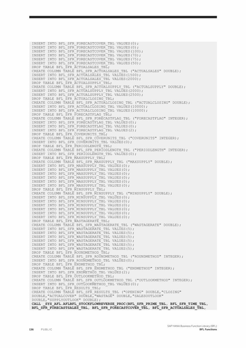
INSERT INTO BFL_SFR_FORECASTCOVER_TBL VALUES(0);INSERT INTO BFL_SFR_FORECASTCOVER_TBL VALUES(0);INSERT INTO BFL_SFR_FORECASTCOVER_TBL VALUES(100);INSERT INTO BFL_SFR_FORECASTCOVER_TBL VALUES(70);INSERT INTO BFL_SFR_FORECASTCOVER_TBL VALUES(75);INSERT INTO BFL_SFR_FORECASTCOVER_TBL VALUES(50);DROP TABLE BFL_SFR_ACTUALSALES_TBL;CREATE COLUMN TABLE BFL_SFR_ACTUALSALES_TBL ("ACTUALSALES" DOUBLE);INSERT INTO BFL_SFR_ACTUALSALES_TBL VALUES(1500);INSERT INTO BFL_SFR_ACTUALSALES_TBL VALUES(2000);DROP TABLE BFL_SFR_ACTUALSUPPLY_TBL;CREATE COLUMN TABLE BFL_SFR_ACTUALSUPPLY_TBL ("ACTUALSUPPLY" DOUBLE);INSERT INTO BFL_SFR_ACTUALSUPPLY_TBL VALUES(2000);INSERT INTO BFL_SFR_ACTUALSUPPLY_TBL VALUES(2500);DROP TABLE BFL_SFR_ACTUALCLOSING_TBL;CREATE COLUMN TABLE BFL_SFR_ACTUALCLOSING_TBL ("ACTUALCLOSING" DOUBLE);INSERT INTO BFL_SFR_ACTUALCLOSING_TBL VALUES(10000);INSERT INTO BFL_SFR_ACTUALCLOSING_TBL VALUES(10000);DROP TABLE BFL_SFR_FORECASTFLAG_TBL;CREATE COLUMN TABLE BFL_SFR_FORECASTFLAG_TBL ("FORECASTFLAG" INTEGER);INSERT INTO BFL_SFR_FORECASTFLAG_TBL VALUES(0);INSERT INTO BFL_SFR_FORECASTFLAG_TBL VALUES(0);INSERT INTO BFL_SFR_FORECASTFLAG_TBL VALUES(2);DROP TABLE BFL_SFR_COVERUNITS_TBL;CREATE COLUMN TABLE BFL_SFR_COVERUNITS_TBL ("COVERUNITS" INTEGER);INSERT INTO BFL_SFR_COVERUNITS_TBL VALUES(0);DROP TABLE BFL_SFR_PERIODLENGTH_TBL;CREATE COLUMN TABLE BFL_SFR_PERIODLENGTH_TBL ("PERIODLENGTH" INTEGER);INSERT INTO BFL_SFR_PERIODLENGTH_TBL VALUES(0);DROP TABLE BFL_SFR_MAXSUPPLY_TBL;CREATE COLUMN TABLE BFL_SFR_MAXSUPPLY_TBL ("MAXSUPPLY" DOUBLE);INSERT INTO BFL_SFR_MAXSUPPLY_TBL VALUES(0);INSERT INTO BFL_SFR_MAXSUPPLY_TBL VALUES(0);INSERT INTO BFL_SFR_MAXSUPPLY_TBL VALUES(0);INSERT INTO BFL_SFR_MAXSUPPLY_TBL VALUES(0);INSERT INTO BFL_SFR_MAXSUPPLY_TBL VALUES(0);INSERT INTO BFL_SFR_MAXSUPPLY_TBL VALUES(0);DROP TABLE BFL_SFR_MINSUPPLY_TBL;CREATE COLUMN TABLE BFL_SFR_MINSUPPLY_TBL ("MINSUPPLY" DOUBLE);INSERT INTO BFL_SFR_MINSUPPLY_TBL VALUES(0);INSERT INTO BFL_SFR_MINSUPPLY_TBL VALUES(0);INSERT INTO BFL_SFR_MINSUPPLY_TBL VALUES(0);INSERT INTO BFL_SFR_MINSUPPLY_TBL VALUES(0);INSERT INTO BFL_SFR_MINSUPPLY_TBL VALUES(0);INSERT INTO BFL_SFR_MINSUPPLY_TBL VALUES(0);DROP TABLE BFL_SFR_WASTAGERATE_TBL;CREATE COLUMN TABLE BFL_SFR_WASTAGERATE_TBL ("WASTAGERATE" DOUBLE);INSERT INTO BFL_SFR_WASTAGERATE_TBL VALUES(5);INSERT INTO BFL_SFR_WASTAGERATE_TBL VALUES(5);INSERT INTO BFL_SFR_WASTAGERATE_TBL VALUES(5);INSERT INTO BFL_SFR_WASTAGERATE_TBL VALUES(5);INSERT INTO BFL_SFR_WASTAGERATE_TBL VALUES(5);INSERT INTO BFL_SFR_WASTAGERATE_TBL VALUES(5);DROP TABLE BFL_SFR_ROUNDMETHOD_TBL;CREATE COLUMN TABLE BFL_SFR_ROUNDMETHOD_TBL ("ROUNDMETHOD" INTEGER);INSERT INTO BFL_SFR_ROUNDMETHOD_TBL VALUES(0);DROP TABLE BFL_SFR_ENDMETHOD_TBL;CREATE COLUMN TABLE BFL_SFR_ENDMETHOD_TBL ("ENDMETHOD" INTEGER);INSERT INTO BFL_SFR_ENDMETHOD_TBL VALUES(2);DROP TABLE BFL_SFR_OUTLOOKMETHOD_TBL;CREATE COLUMN TABLE BFL_SFR_OUTLOOKMETHOD_TBL ("OUTLOOKMETHOD" INTEGER);INSERT INTO BFL_SFR_OUTLOOKMETHOD_TBL VALUES(0);DROP TABLE BFL_SFR_RESULTS_TBL;CREATE COLUMN TABLE BFL_SFR_RESULTS_TBL ("OPENING" DOUBLE,"CLOSING" DOUBLE,"ACTUALCOVER" DOUBLE,"WASTAGE" DOUBLE,"SALESOUTLOOK" DOUBLE,"SUPPLYOUTLOOK" DOUBLE); CALL _SYS_AFL.AFLBFL_STOCKFLOWREVERSE_PROC(BFL_SFR_PRIME_TBL, BFL_SFR_TIME_TBL, BFL_SFR_FORECASTSALES_TBL, BFL_SFR_FORECASTCOVER_TBL, BFL_SFR_ACTUALSALES_TBL,
136 P U B L I CSAP HANA Business Function Library (BFL)
BFL Functions

BFL_SFR_ACTUALSUPPLY_TBL, BFL_SFR_ACTUALCLOSING_TBL, BFL_SFR_FORECASTFLAG_TBL, BFL_SFR_COVERUNITS_TBL, BFL_SFR_PERIODLENGTH_TBL , BFL_SFR_MAXSUPPLY_TBL, BFL_SFR_MINSUPPLY_TBL, BFL_SFR_WASTAGERATE_TBL, BFL_SFR_ROUNDMETHOD_TBL, BFL_SFR_ENDMETHOD_TBL, BFL_SFR_OUTLOOKMETHOD_TBL, BFL_SFR_RESULTS_TBL ) WITH OVERVIEW; SELECT * FROM BFL_SFR_RESULTS_TBL;
3.47 Stock Flow Batch
This function enables the use of batch quantities when calculating stock flow.
Supply Outlook=Stock Flow Reverse(Prime; Opening Stock; Forecast Sales; Forecast Cover; Closing Stock; Actual Sales; Actual Cover; Actual Supply; Actual Closing; Forecast flag; Cover Units; Period Length; Max Supply; Min Supply; Batch Quantity; Minimum Method; % Wastage; Wastage; Rounding Method; End Method; Outlook Method; Sales Outlook)
Methods
See the Stock Flow Function for complete information on methods.
Batch Quantity
When {Batch Quantity} is non-zero, the {Supply Outlook} will be rounded up to the next integer multiple of {Batch Quantity}. Stock Flow Reverse has more information about other inputs and calculations.
Minimum Method
Applies to {Supply Outlook} in forecast periods.
It modifies the effect of {Min Supply}.
Minimum, Maximum and batch size
Stock Flow Batch resolves inconsistent inputs in the following manner:
● If {Min Supply} > 0 and {Batch Size} > 0, then round {Min Supply} up to the next integer multiple of {Batch Size}.
● If {Batch Size} > 0 and {Max Supply} > 0, then round {Max Supply} down to the next integer multiple of {Batch Size}.
● If {Min Supply} > {Max Supply}, then set {Max Supply} = {Min Supply}.
Signature
Input Tables
SAP HANA Business Function Library (BFL)BFL Functions P U B L I C 137

Table 110:
Name Direction Number of Columns
Column Type Column Name Description
Prime Input Table 1 Double PRIME Prime - opening stock of the first period.
Time Input Table 1 String TIME The calculated time.
Forecast Sales Input Table 1 Double FORECASTSALES Forecast sales will be used in the period containing the switchover date and thereafter. Prior to the switchover date there is no forecast – only actual.
Forecast Cover Input Table 1 Double FORECASTCOVER The forecast stock cover. How many days/periods of future sales the closing stock should support. 100 sets Closing Stock at such a level that it lasts 100 days based on Sales Outlook.
Actual Sales Input Table 1 Double ACTUALSALES Actual Sales input for historic periods only.
Actual Supply Input Table 1 Double ACTUALSUPPLY Actual Supply input for historic periods only.
Actual Closing Input Table 1 Double ACTUALCLOSING Actual Closing Stock input for historic periods only.
Forecast Flag Input Table 1 Int FORECASTFLAG Enter a flag to act as a Year over Year Difference switchover date on each page. The first value > 1 indicates the start of forecast periods.
138 P U B L I CSAP HANA Business Function Library (BFL)
BFL Functions

Name Direction Number of Columns
Column Type Column Name Description
Cover Units Input Table 1 Int COVERUNITS Identifies the measure for Stock Cover in terms of future sales. Days: Use calendar days. Default. Units: Use custom units from the item Period Length. Periods: Use number of periods. Each detail item in the timescale field is a period.
Period Length Input Table 1 Int PERIODLENGTH Available if you want to use non-standard calendar period lengths. For example: 4 - 4 - 5 for weeks in each period. Period Length will be ignored unless you set Cover Units=Period.
Max Supply Input Table 1 Double MAXSUPPLY Physical limitations (constraints) to the maximum supply available to increase stock levels (warehouse space, etc). If left blank, the default is for Max Supply to be allowed to go to infinity.
Min Supply Input Table 1 Double MINSUPPLY Limitation to the flow out of stock.
Batch Quantity Input Table 1 Double BATCHQUANTITY When {Batch Quantity} is non-zero, the {Supply Outlook} will be rounded up to the next integer multiple of {Batch Quantity}. Stock Flow Reverse has more information about other inputs and calculations.
SAP HANA Business Function Library (BFL)BFL Functions P U B L I C 139

Name Direction Number of Columns
Column Type Column Name Description
Wastage Rate Input Table 1 Double WASTAGERATE Changes in stock due to shrinkage (not explained by sales and supply). Wastage is = to % Wastage applied to the Opening Stock.
Rounding Method Input Table 1 Int ROUNDMETHOD DNR: Do not round. This is the default if left blank (no partial units, discrete units only). Round: Round each element (process). Preserve Sum: Preserve the sum by changing the most obvious element(s), where rounded value is furthest from original value. Preserve Sum YoY: Preserve the sum by rounding cumulated data and then taking the Year over Year Difference (the default).
End Method Input Table 1 Int ENDMETHOD Integer Constant: The number of periods over which to average sales when projecting beyond the last period in the timescale. This is used in the closing stock calculation toward the end of the timescale. N periods: Use the average of the last 3 periods to project sales forward.
140 P U B L I CSAP HANA Business Function Library (BFL)
BFL Functions

Name Direction Number of Columns
Column Type Column Name Description
Outlook Method Input Table 1 Int OUTLOOKMETHOD
How forecast sales input is used to provide future sales outlook. Default: Use Forecast Sales from the period containing the switchover date onwards, Actual Sales prior to this (the default method). Restrict: Restrict future sales if closing stock goes negative.
Output Table
Table 111:
Name Direction Number of Columns
Column Type Column Name Description
Result Output Table 6 Double OPENING Opening Stock. Fed from the Closing Stock of the previous period.
Double CLOSING Closing Stock. Actual Closing Stock prior to the switchover date; the level required to meet the Forecast Stock Cover thereafter.
Double ACTUALCOVER Actual Stock Cover. How many days/periods of future sales the Closing Stock actually does support.
Double WASTAGE Changes in stock due to shrinkage (not explained by sales and supply). Wastage is = to % Wastage applied to the Opening Stock.
SAP HANA Business Function Library (BFL)BFL Functions P U B L I C 141

Name Direction Number of Columns
Column Type Column Name Description
Double SALESOUTLOOK Sales Outlook is equal to the Actual Sales history prior to the switchover date, Forecast Sales thereafter. See Outlook Method.
Double SUPPLYOUTLOOK The supply in future periods required to meet forecast stock cover based on forecast sales. The supply is subject to the constraints of Min and Max Supply. Prior to the switchover date, Supply Outlook equals Actual Supply.
Example
Assume that:
● BFL_TEST is a schema belonging to USER1; and● USER1 has been assigned the AFL__SYS_AFL_AFLBFL_EXECUTE or
AFL__SYS_AFL_AFLBFL_EXECUTE_WITH_GRANT_OPTION role.
SET SCHEMA BFL_TEST; DROP TABLE BFL_SFB_PRIME_TBL;CREATE COLUMN TABLE BFL_SFB_PRIME_TBL ("PRIME" DOUBLE);INSERT INTO BFL_SFB_PRIME_TBL VALUES(10000);DROP TABLE BFL_SFB_TIME_TBL;CREATE COLUMN TABLE BFL_SFB_TIME_TBL ("TIME" VARCHAR(255));INSERT INTO BFL_SFB_TIME_TBL VALUES('20100801');INSERT INTO BFL_SFB_TIME_TBL VALUES('20100912');INSERT INTO BFL_SFB_TIME_TBL VALUES('20101020');INSERT INTO BFL_SFB_TIME_TBL VALUES('20101130');INSERT INTO BFL_SFB_TIME_TBL VALUES('20110105');INSERT INTO BFL_SFB_TIME_TBL VALUES('20110220');DROP TABLE BFL_SFB_FORECASTSALES_TBL;CREATE COLUMN TABLE BFL_SFB_FORECASTSALES_TBL ("FORECASTSALES" DOUBLE);INSERT INTO BFL_SFB_FORECASTSALES_TBL VALUES(0);INSERT INTO BFL_SFB_FORECASTSALES_TBL VALUES(0);INSERT INTO BFL_SFB_FORECASTSALES_TBL VALUES(2500);INSERT INTO BFL_SFB_FORECASTSALES_TBL VALUES(3000);INSERT INTO BFL_SFB_FORECASTSALES_TBL VALUES(2500);INSERT INTO BFL_SFB_FORECASTSALES_TBL VALUES(3500);DROP TABLE BFL_SFB_FORECASTCOVER_TBL;CREATE COLUMN TABLE BFL_SFB_FORECASTCOVER_TBL ("FORECASTCOVER" DOUBLE);
142 P U B L I CSAP HANA Business Function Library (BFL)
BFL Functions

INSERT INTO BFL_SFB_FORECASTCOVER_TBL VALUES(0);INSERT INTO BFL_SFB_FORECASTCOVER_TBL VALUES(0);INSERT INTO BFL_SFB_FORECASTCOVER_TBL VALUES(100);INSERT INTO BFL_SFB_FORECASTCOVER_TBL VALUES(70);INSERT INTO BFL_SFB_FORECASTCOVER_TBL VALUES(75);INSERT INTO BFL_SFB_FORECASTCOVER_TBL VALUES(50);DROP TABLE BFL_SFB_ACTUALSALES_TBL;CREATE COLUMN TABLE BFL_SFB_ACTUALSALES_TBL ("ACTUALSALES" DOUBLE);INSERT INTO BFL_SFB_ACTUALSALES_TBL VALUES(1500);INSERT INTO BFL_SFB_ACTUALSALES_TBL VALUES(2000);DROP TABLE BFL_SFB_ACTUALSUPPLY_TBL;CREATE COLUMN TABLE BFL_SFB_ACTUALSUPPLY_TBL ("ACTUALSUPPLY" DOUBLE);INSERT INTO BFL_SFB_ACTUALSUPPLY_TBL VALUES(2000);INSERT INTO BFL_SFB_ACTUALSUPPLY_TBL VALUES(2500);DROP TABLE BFL_SFB_ACTUALCLOSING_TBL;CREATE COLUMN TABLE BFL_SFB_ACTUALCLOSING_TBL ("ACTUALCLOSING" DOUBLE);INSERT INTO BFL_SFB_ACTUALCLOSING_TBL VALUES(10000);INSERT INTO BFL_SFB_ACTUALCLOSING_TBL VALUES(10000);DROP TABLE BFL_SFB_FORECASTFLAG_TBL;CREATE COLUMN TABLE BFL_SFB_FORECASTFLAG_TBL ("FORECASTFLAG" INTEGER);INSERT INTO BFL_SFB_FORECASTFLAG_TBL VALUES(0);INSERT INTO BFL_SFB_FORECASTFLAG_TBL VALUES(0);INSERT INTO BFL_SFB_FORECASTFLAG_TBL VALUES(2);DROP TABLE BFL_SFB_COVERUNITS_TBL;CREATE COLUMN TABLE BFL_SFB_COVERUNITS_TBL ("COVERUNITS" INTEGER);INSERT INTO BFL_SFB_COVERUNITS_TBL VALUES(0);DROP TABLE BFL_SFB_PERIODLENGTH_TBL;CREATE COLUMN TABLE BFL_SFB_PERIODLENGTH_TBL ("PERIODLENGTH" INTEGER);INSERT INTO BFL_SFB_PERIODLENGTH_TBL VALUES(0);DROP TABLE BFL_SFB_MAXSUPPLY_TBL;CREATE COLUMN TABLE BFL_SFB_MAXSUPPLY_TBL ("MAXSUPPLY" DOUBLE);INSERT INTO BFL_SFB_MAXSUPPLY_TBL VALUES(0);INSERT INTO BFL_SFB_MAXSUPPLY_TBL VALUES(0);INSERT INTO BFL_SFB_MAXSUPPLY_TBL VALUES(0);INSERT INTO BFL_SFB_MAXSUPPLY_TBL VALUES(0);INSERT INTO BFL_SFB_MAXSUPPLY_TBL VALUES(0);INSERT INTO BFL_SFB_MAXSUPPLY_TBL VALUES(0);DROP TABLE BFL_SFB_MINSUPPLY_TBL;CREATE COLUMN TABLE BFL_SFB_MINSUPPLY_TBL ("MINSUPPLY" DOUBLE);INSERT INTO BFL_SFB_MINSUPPLY_TBL VALUES(0);INSERT INTO BFL_SFB_MINSUPPLY_TBL VALUES(0);INSERT INTO BFL_SFB_MINSUPPLY_TBL VALUES(0);INSERT INTO BFL_SFB_MINSUPPLY_TBL VALUES(0);INSERT INTO BFL_SFB_MINSUPPLY_TBL VALUES(0);INSERT INTO BFL_SFB_MINSUPPLY_TBL VALUES(0);DROP TABLE BFL_SFB_BATCHQUANTITY_TBL;CREATE COLUMN TABLE BFL_SFB_BATCHQUANTITY_TBL("BATCHQUANTITY" DOUBLE);INSERT INTO BFL_SFB_BATCHQUANTITY_TBL VALUES(0);INSERT INTO BFL_SFB_BATCHQUANTITY_TBL VALUES(0);INSERT INTO BFL_SFB_BATCHQUANTITY_TBL VALUES(0);INSERT INTO BFL_SFB_BATCHQUANTITY_TBL VALUES(0);INSERT INTO BFL_SFB_BATCHQUANTITY_TBL VALUES(0);INSERT INTO BFL_SFB_BATCHQUANTITY_TBL VALUES(0);DROP TABLE BFL_SFB_WASTAGERATE_TBL;CREATE COLUMN TABLE BFL_SFB_WASTAGERATE_TBL ("WASTAGERATE" DOUBLE);INSERT INTO BFL_SFB_WASTAGERATE_TBL VALUES(5);INSERT INTO BFL_SFB_WASTAGERATE_TBL VALUES(5);INSERT INTO BFL_SFB_WASTAGERATE_TBL VALUES(5);INSERT INTO BFL_SFB_WASTAGERATE_TBL VALUES(5);INSERT INTO BFL_SFB_WASTAGERATE_TBL VALUES(5);INSERT INTO BFL_SFB_WASTAGERATE_TBL VALUES(5);DROP TABLE BFL_SFB_ROUNDMETHOD_TBL;CREATE COLUMN TABLE BFL_SFB_ROUNDMETHOD_TBL ("ROUNDMETHOD" INTEGER);INSERT INTO BFL_SFB_ROUNDMETHOD_TBL VALUES(0);DROP TABLE BFL_SFB_ENDMETHOD_TBL;CREATE COLUMN TABLE BFL_SFB_ENDMETHOD_TBL ("ENDMETHOD" INTEGER);INSERT INTO BFL_SFB_ENDMETHOD_TBL VALUES(2);DROP TABLE BFL_SFB_OUTLOOKMETHOD_TBL;
SAP HANA Business Function Library (BFL)BFL Functions P U B L I C 143

CREATE COLUMN TABLE BFL_SFB_OUTLOOKMETHOD_TBL ("OUTLOOKMETHOD" INTEGER);INSERT INTO BFL_SFB_OUTLOOKMETHOD_TBL VALUES(0);DROP TABLE BFL_SFB_RESULTS_TBL;CREATE COLUMN TABLE BFL_SFB_RESULTS_TBL ("OPENING" DOUBLE,"CLOSING" DOUBLE,"ACTUALCOVER" DOUBLE,"WASTAGE" DOUBLE,"SALESOUTLOOK" DOUBLE,"SUPPLYOUTLOOK" DOUBLE); CALL _SYS_AFL.AFLBFL_STOCKFLOWBATCH_PROC(BFL_SFB_PRIME_TBL, BFL_SFB_TIME_TBL, BFL_SFB_FORECASTSALES_TBL, BFL_SFB_FORECASTCOVER_TBL, BFL_SFB_ACTUALSALES_TBL, BFL_SFB_ACTUALSUPPLY_TBL, BFL_SFB_ACTUALCLOSING_TBL, BFL_SFB_FORECASTFLAG_TBL, BFL_SFB_COVERUNITS_TBL, BFL_SFB_PERIODLENGTH_TBL , BFL_SFB_MAXSUPPLY_TBL, BFL_SFB_MINSUPPLY_TBL, BFL_SFB_BATCHQUANTITY_TBL, BFL_SFB_WASTAGERATE_TBL, BFL_SFB_ROUNDMETHOD_TBL, BFL_SFB_ENDMETHOD_TBL, BFL_SFB_OUTLOOKMETHOD_TBL, BFL_SFB_RESULTS_TBL ) WITH OVERVIEW; SELECT * FROM BFL_SFB_RESULTS_TBL;
3.48 Time
This function returns the information requested by the option you have input. It is one of the most time consuming elements in FPM or simulation because of the relevance of specific periods. Scripting of time, particularly in excel driven formats (such as BPC) can be extremely costly and extremely difficult to maintain. If any modeling requires modification of the time series, the condition becomes worse.
Timescale standard:
● Start of a period = Midnight of the first day● Middle of a period = Noon or midnight (This depends on the number of days in the period)● End of a period = Midnight on the last day (also the start of the next day)
Signature
Input Tables
Table 112:
Name Direction Number of Columns
Column Type Column Name Description
Time Scale Input Table 1 Double TIMESCALE Input amount
Start Date Input Table 1 Double STARTDATE The date start to calculate
Switchover Input Table 1 Double SWITCHOVER Switchover date
144 P U B L I CSAP HANA Business Function Library (BFL)
BFL Functions

Name Direction Number of Columns
Column Type Column Name Description
Time information Input Table 1 Double TIMEINFORMATION
The option you require for time information. Detail information shown below: Now(0) Last(1) Start(2) Mid(3) End(4) Days(5) IID(6) Current(7) Switchover(8) Actual(9): Cycle(10): Period(11): First(12): Last(13): Actual(14): Min(15): Method(16)
Output Table
Table 113:
Name Direction Number of Columns
Column Type Column Name Description
Result Output Table 1 String TIME Returns time-related information
Specification of Method
Now(0): Current system date and time
Last(1): Last Save
Start(2): the date and time at the start of this period
Mid(3): the date and time at the middle of this period
End(4): the date and time at the end of this period
Days(5): the number of days in this period
IID(6)
Current(7): Sets a flag = 1 in the period containing system date
Switchover(8): Sets a flag =1 in the period containing switchover date
Actual(9): Sets a flag =1 in periods up to, but not including, the period containing the system date (current)
Cycle(10): The number of periods like this in a year to the nearest whole number (minimum 1)
Period(11): Number the periods within a year, starting again at 1 each year and counting up until it reaches the total number of periods in the year (as defined in ‘cycle’)
First(12): Sets a flag =1 in the first period of every timescale subtotal
SAP HANA Business Function Library (BFL)BFL Functions P U B L I C 145

Last(13): Sets a flag =1 in the last period of every timescale subtotal
Actual(14): Sets a flag =1 in periods up to, but not including, the period containing the switchover date
Min(15): the date and time 1 minute before midnight on last day of period
Method(16): the middle of each period in year units, where 2003.5 means the middle of 2003. It is used by Cycles as its measure of time
Example
Assume that:
● BFL_TEST is a schema belonging to USER1; and● USER1 has been assigned the AFL__SYS_AFL_AFLBFL_EXECUTE or
AFL__SYS_AFL_AFLBFL_EXECUTE_WITH_GRANT_OPTION role.
SET SCHEMA BFL_TEST; DROP TABLE BFL_TIME_TIMESCALE_TBL;CREATE COLUMN TABLE BFL_TIME_TIMESCALE_TBL ( "TIMESCALE" DOUBLE ) ;INSERT INTO BFL_TIME_TIMESCALE_TBL VALUES (0) ;DROP TABLE BFL_TIME_STARTDATE_TBL; CREATE COLUMN TABLE BFL_TIME_STARTDATE_TBL ( "STARTDATE" DOUBLE ) ;INSERT INTO BFL_TIME_STARTDATE_TBL VALUES ('20040228') ;DROP TABLE BFL_TIME_SWITCHOVER_TBL;CREATE COLUMN TABLE BFL_TIME_SWITCHOVER_TBL ( "SWITCHOVER" DOUBLE ) ;INSERT INTO BFL_TIME_SWITCHOVER_TBL VALUES ('20040307') ;DROP TABLE BFL_TIME_TIMEINFORMATION_TBL;CREATE COLUMN TABLE BFL_TIME_TIMEINFORMATION_TBL ( "TIMEINFORMATION" DOUBLE ) ;INSERT INTO BFL_TIME_TIMEINFORMATION_TBL VALUES (4) ;DROP TABLE BFL_TIME_TIME_TBL; CREATE COLUMN TABLE BFL_TIME_TIME_TBL ( "TIME" VARCHAR(255)) ; CALL _SYS_AFL.AFLBFL_TIME_PROC(BFL_TIME_TIMESCALE_TBL, BFL_TIME_STARTDATE_TBL, BFL_TIME_SWITCHOVER_TBL, BFL_TIME_TIMEINFORMATION_TBL, BFL_TIME_TIME_TBL) WITH OVERVIEW; SELECT * FROM BFL_TIME_TIME_TBL;
3.49 Time Sum
This function needs to use the generator mentioned in Calling BFL Functions [page 7].
This function allows you to accumulate an expense over a specified number of periods in advance or in arrears. It can also be used in conjunction with the Delay function to convert an expense stream in the P&L firstly into invoice amounts, then into cash payments.
Formula
Time Sum=Time Sum (Amount, Periods, Arrears/Advance, End, Override, Days in Period, Indicator)
146 P U B L I CSAP HANA Business Function Library (BFL)
BFL Functions

Signature
Input Tables
Table 114:
Name Direction Number of Columns
Column Type Column Name Description
Data Input Table 1 Double DATE The amount to accrue.
Number Periods Input Table 1 Double NUMPERIODS The number of periods to add up to determine the size of the bill. For example, if you enter 3, it accumulates three periods. This parameter reads the Advance/Arrears parameter to determine whether to count the periods forward (Advance) or backward (Arrears). Periods are processed in chronological order, regardless of the sequence of the periods.
Methods Input Table 3 Double METHOD1 Arrears/ Advance type:
● In arrears● In advance
Double METHOD2 End type:
● Zero (default)● Average● Replicate● Override -The
override is used even if the number of periods is 0.
● Spare
Double METHOD2 Override value.
Days Input Table 1 Double DAYS Length of period in days.
SAP HANA Business Function Library (BFL)BFL Functions P U B L I C 147

Name Direction Number of Columns
Column Type Column Name Description
Config Input Table 1 Double CONFIG Has six rows, each rows specify as below:
● 0: 0, days is not used; 1, days is used; 2, days is not used
● 1: First calculated month
● 2: To calculate month length
● 3: First calculated year
● 4: Length of Year
● 5: Zero or non-zero, if zero, days is not used
Output Table
Table 115:
Name Direction Number of Columns
Column Type Column Name Description
Result Output Table 1 Double TIMESUM The cash payments
Example
Assume that:
● BFL_TEST is a schema belonging to USER1; and● USER1 has been assigned the AFLPM_CREATOR_ERASER_EXECUTE role; and● USER1 has been assigned the AFL__SYS_AFL_AFLBFL_EXECUTE or
AFL__SYS_AFL_AFLBFL_EXECUTE_WITH_GRANT_OPTION role.
SET SCHEMA BFL_TEST; DROP TYPE BFL_TMSM_DATA_T;CREATE TYPE BFL_TMSM_DATA_T AS TABLE("DATA" DOUBLE);DROP TYPE BFL_TMSM_NUMPERIODS_T;CREATE TYPE BFL_TMSM_NUMPERIODS_T AS TABLE("NUMPERIODS" DOUBLE);DROP TYPE BFL_TMSM_METHOD_T;CREATE TYPE BFL_TMSM_METHOD_T AS TABLE("METHOD1" DOUBLE, "METHOD2" DOUBLE, "METHOD3" DOUBLE);DROP TYPE BFL_TMSM_DAYS_T;CREATE TYPE BFL_TMSM_DAYS_T AS TABLE("DAYS" DOUBLE);
148 P U B L I CSAP HANA Business Function Library (BFL)
BFL Functions

DROP TYPE BFL_TMSM_CONFIG_T;CREATE TYPE BFL_TMSM_CONFIG_T AS TABLE("CONFIG" DOUBLE);DROP TYPE BFL_TMSM_RESULT_T;CREATE TYPE BFL_TMSM_RESULT_T AS TABLE("TIMESUM" DOUBLE);DROP table BFL_TMSM_PDATA_TBL;CREATE column table BFL_TMSM_PDATA_TBL("POSITION" INT,"SCHEMA_NAME" NVARCHAR(256),"TYPE_NAME" NVARCHAR(256), ”PARAMETER_TYPE” VARCHAR(7));insert into BFL_TMSM_PDATA_TBL values (1,'BFL_TEST’,’BFL_TMSM_DATA_T', 'IN'); insert into BFL_TMSM_PDATA_TBL values (2,'BFL_TEST’,’BFL_TMSM_NUMPERIODS_T', 'IN'); insert into BFL_TMSM_PDATA_TBL values (3,'BFL_TEST’,’BFL_TMSM_METHOD_T', 'IN'); insert into BFL_TMSM_PDATA_TBL values (4,'BFL_TEST’,’BFL_TMSM_DAYS_T', 'IN');insert into BFL_TMSM_PDATA_TBL values (5,'BFL_TEST’,’BFL_TMSM_CONFIG_T', 'IN'); insert into BFL_TMSM_PDATA_TBL values (6,'BFL_TEST’,’BFL_TMSM_RESULT_T', 'OUT'); call SYS.AFLLANG_WRAPPER_PROCEDURE_DROP('BFL_TEST’,'AFLBFL_TIMESUM_PROC'); call SYS.AFLLANG_WRAPPER_PROCEDURE_CREATE('AFLBFL','TIMESUM','TEST_BFL', 'AFLBFL_TIMESUM_PROC',BFL_TMSM_PDATA_TBL); DROP TABLE BFL_TMSM_DATA_TBL;CREATE COLUMN TABLE BFL_TMSM_DATA_TBL ( "DATA" DOUBLE ) ;INSERT INTO BFL_TMSM_DATA_TBL VALUES (30) ;INSERT INTO BFL_TMSM_DATA_TBL VALUES (40) ;INSERT INTO BFL_TMSM_DATA_TBL VALUES (40) ;INSERT INTO BFL_TMSM_DATA_TBL VALUES (300) ;INSERT INTO BFL_TMSM_DATA_TBL VALUES (400) ;INSERT INTO BFL_TMSM_DATA_TBL VALUES (500) ; DROP TABLE BFL_TMSM_NUMPERIODS_TBL;CREATE COLUMN TABLE BFL_TMSM_NUMPERIODS_TBL ( "NUMPERIODS" DOUBLE ) ;INSERT INTO BFL_TMSM_NUMPERIODS_TBL VALUES (0) ;INSERT INTO BFL_TMSM_NUMPERIODS_TBL VALUES (3) ;INSERT INTO BFL_TMSM_NUMPERIODS_TBL VALUES (0) ;INSERT INTO BFL_TMSM_NUMPERIODS_TBL VALUES (12) ;DROP TABLE BFL_TMSM_METHOD_TBL;CREATE COLUMN TABLE BFL_TMSM_METHOD_TBL ( "METHOD1" DOUBLE ,"METHOD2" DOUBLE,"METHOD3" DOUBLE);INSERT INTO BFL_TMSM_METHOD_TBL VALUES (1, 0, 0) ;DROP TABLE BFL_TMSM_DAYS_TBL;CREATE COLUMN TABLE BFL_TMSM_DAYS_TBL ( "DAYS" DOUBLE ) ;INSERT INTO BFL_TMSM_DAYS_TBL VALUES (30) ;INSERT INTO BFL_TMSM_DAYS_TBL VALUES (30) ;INSERT INTO BFL_TMSM_DAYS_TBL VALUES (30) ;INSERT INTO BFL_TMSM_DAYS_TBL VALUES (360) ;INSERT INTO BFL_TMSM_DAYS_TBL VALUES (360) ;INSERT INTO BFL_TMSM_DAYS_TBL VALUES (360) ;DROP TABLE BFL_TMSM_CONFIG_TBL; CREATE COLUMN TABLE BFL_TMSM_CONFIG_TBL ( "CONFIG" DOUBLE) ;INSERT INTO BFL_TMSM_CONFIG_TBL VALUES (1) ;INSERT INTO BFL_TMSM_CONFIG_TBL VALUES (10) ;INSERT INTO BFL_TMSM_CONFIG_TBL VALUES (1) ;INSERT INTO BFL_TMSM_CONFIG_TBL VALUES (0) ;INSERT INTO BFL_TMSM_CONFIG_TBL VALUES (3) ;INSERT INTO BFL_TMSM_CONFIG_TBL VALUES (3) ;DROP TABLE BFL_TMSM_TIMESUM_TBL; CREATE COLUMN TABLE BFL_TMSM_TIMESUM_TBL ( "TIMESUM" DOUBLE) ; CALL BFL_TEST.AFLBFL_TIMESUM_PROC(BFL_TMSM_DATA_TBL, BFL_TMSM_NUMPERIODS_TBL, BFL_TMSM_METHOD_TBL, BFL_TMSM_DAYS_TBL, BFL_TMSM_CONFIG_TBL, BFL_TMSM_TIMESUM_TBL) WITH OVERVIEW; SELECT * FROM BFL_TMSM_TIMESUM_TBL;
3.50 Transform
This function provides some angles and trigonometry functions for users based on different methods. It can be used when the Cycles function does not meet the functionality you need.
SAP HANA Business Function Library (BFL)BFL Functions P U B L I C 149

Signature
Input Tables
Table 116:
Name Direction Number of Columns
Column Type Column Name Description
Input Input Table 1 Double VALUE Input value, varies with the method, for example: angle measured in radians.
Method Input Table 1 Double VALUE Methods: 0=No Change; 1=Sine; 2=Cosine; 3=Tangent;4=(1+input^2)^.5;5=sinh;6=cosh;7=tanh; 8=Degrees to radians; ...
Output Table
Table 117:
Name Direction Number of Columns
Column Type Column Name Description
Result Output Table 1 Double TRANSFORM Transformations for time series
Example
Assume that:
● BFL_TEST is a schema belonging to USER1; and● USER1 has been assigned the AFL__SYS_AFL_AFLBFL_EXECUTE or
AFL__SYS_AFL_AFLBFL_EXECUTE_WITH_GRANT_OPTION role.
SET SCHEMA BFL_TEST; DROP TABLE BFL_TSFM_INPUT_TBL ;CREATE COLUMN TABLE BFL_TSFM_INPUT_TBL ( "VALUE" DOUBLE ) ;INSERT INTO BFL_TSFM_INPUT_TBL VALUES (10) ;DROP TABLE BFL_TSFM_METHOD_TBL ;CREATE COLUMN TABLE BFL_TSFM_METHOD_TBL ( "VALUE" DOUBLE ) ;INSERT INTO BFL_TSFM_METHOD_TBL VALUES (7) ;DROP TABLE BFL_TSFM_RESULTS_TBL ;CREATE COLUMN TABLE BFL_TSFM_RESULTS_TBL ("TRANSFORM" DOUBLE) ; CALL _SYS_AFL.AFLBFL_TRANSFORM_PROC(BFL_TSFM_INPUT_TBL, BFL_TSFM_METHOD_TBL, BFL_TSFM_RESULTS_TBL) WITH OVERVIEW; SELECT * FROM BFL_TSFM_RESULTS_TBL;
150 P U B L I CSAP HANA Business Function Library (BFL)
BFL Functions

3.51 Volume Driver
This function calculates the year-over-year percentage difference for each volume driver. A volume driver is entered as a percentage and a bandwidth. The bandwidth should be a positive number. The bandwidth of the first volume driver always starts at zero.
After allocating percentage to all non-zero bandwidth, the remaining percentage will be applied to any residue.
Formula
Volume Driver result = Volume Driver(Value, Volume Driver1 %, Volume Driver1, Volume Driver2 %, Volume Driver2, Volume Driver3 %, Volume Driver3 …)
Signature
Input Tables
Table 118:
Name Direction Number of Columns
Column Type Column Name Description
Salary Input Table 1 Double SALARY Input amount
Percent Input Table 1 Double PERCENT Percentage to be applied, starting at zero
Bandwidth Input Table 1 Double BANDWIDTH Bandwidth value
Output Table
Table 119:
Name Direction Number of Columns
Column Type Column Name Description
Result Output Table 1 Double OVERHEAD Calculated volume driver result
Example
Assume that:
● BFL_TEST is a schema belonging to USER1; and
SAP HANA Business Function Library (BFL)BFL Functions P U B L I C 151

● USER1 has been assigned the AFL__SYS_AFL_AFLBFL_EXECUTE or AFL__SYS_AFL_AFLBFL_EXECUTE_WITH_GRANT_OPTION role.
SET SCHEMA BFL_TEST; DROP TABLE BFL_VD_VALUES_TBL;CREATE COLUMN TABLE BFL_VD_VALUES_TBL ( "SALARY" DOUBLE );INSERT INTO BFL_VD_VALUES_TBL VALUES (2000);INSERT INTO BFL_VD_VALUES_TBL VALUES (15000);INSERT INTO BFL_VD_VALUES_TBL VALUES (25000);INSERT INTO BFL_VD_VALUES_TBL VALUES (35000);INSERT INTO BFL_VD_VALUES_TBL VALUES (45000);DROP TABLE BFL_VD_PERCENTS_TBL;CREATE COLUMN TABLE BFL_VD_PERCENTS_TBL ( "PERCENT" DOUBLE );INSERT INTO BFL_VD_PERCENTS_TBL VALUES (0);INSERT INTO BFL_VD_PERCENTS_TBL VALUES (0.2);INSERT INTO BFL_VD_PERCENTS_TBL VALUES (0.4);DROP TABLE BFL_VD_BANDWITHS_TBL;CREATE COLUMN TABLE BFL_VD_BANDWITHS_TBL ( "BANDWIDTH" DOUBLE );INSERT INTO BFL_VD_BANDWITHS_TBL VALUES (3000);INSERT INTO BFL_VD_BANDWITHS_TBL VALUES (27000);DROP TABLE BFL_VD_RESULTS_TBL;CREATE COLUMN TABLE BFL_VD_RESULTS_TBL ( "OVERHEAD" DOUBLE); CALL _SYS_AFL.AFLBFL_VOLUMEDRIVER_PROC(BFL_VD_VALUES_TBL, BFL_VD_PERCENTS_TBL, BFL_VD_BANDWITHS_TBL, BFL_VD_RESULTS_TBL) WITH OVERVIEW; SELECT * FROM BFL_VD_RESULTS_TBL;
3.52 Year-Over-Year Difference
This function calculates the year-over -year difference between the current and previous one time period. The function result can be a percentage, proportion, or actual amount.
Formula
Three formulas are required by the Business function for percentage, actual number, or proportion respectively.
Year over Year Difference = Year over Year Difference (Base; Style)
For percentage:
Year over Year Difference, period n = Year over Year Difference (Base; %) = 100*(((Base, period n) - (Base period n-1))/(Base, period n))
For actual amount:
Year over Year Difference, period n = Year over Year Difference (Base; a) = (Base, period n) - (Base, period n-1)
For proportion:
Year over Year Difference, period n = Year over Year Difference ({Base Sales; p) = (Base, period n)/(Base, period n-1)
152 P U B L I CSAP HANA Business Function Library (BFL)
BFL Functions

Signature
Input Tables
Table 120:
Name Direction Number of Columns
Column Type Column Name Description
Base Input Table 1 Double BASE The data to compare
Style Input Table 1 Double STYLE 0: Percent Year over Year Difference 1: Arithmetic Year over Year Difference 2: Proportion Year over Year Difference
Output Table
Table 121:
Name Direction Number of Columns
Column Type Column Name Description
Result Output Table 1 Double DIFFERENCE The Year over Year Difference
Example
Assume that:
● BFL_TEST is a schema belonging to USER1; and● USER1 has been assigned the AFL__SYS_AFL_AFLBFL_EXECUTE or
AFL__SYS_AFL_AFLBFL_EXECUTE_WITH_GRANT_OPTION role.
SET SCHEMA BFL_TEST; DROP TABLE BFL_YOYD_BASE_TBL;CREATE COLUMN TABLE BFL_YOYD_BASE_TBL( "BASE" DOUBLE ) ;INSERT INTO BFL_YOYD_BASE_TBL VALUES (1000) ;INSERT INTO BFL_YOYD_BASE_TBL VALUES (2000) ;INSERT INTO BFL_YOYD_BASE_TBL VALUES (4000) ;INSERT INTO BFL_YOYD_BASE_TBL VALUES (5000) ;INSERT INTO BFL_YOYD_BASE_TBL VALUES (2000) ;INSERT INTO BFL_YOYD_BASE_TBL VALUES (1000) ;INSERT INTO BFL_YOYD_BASE_TBL VALUES (0) ;DROP TABLE BFL_YOYD_STYLE_TBL;CREATE COLUMN TABLE BFL_YOYD_STYLE_TBL( "STYLE" INT);INSERT INTO BFL_YOYD_STYLE_TBL VALUES (0) ;DROP TABLE BFL_YOYD_DIFFERENCE_TBL;CREATE COLUMN TABLE BFL_YOYD_DIFFERENCE_TBL( "DIFFERENCE" DOUBLE) ; CALL _SYS_AFL.AFLBFL_YEAROVERYEARDIFFERENCE_PROC(BFL_YOYD_BASE_TBL, BFL_YOYD_STYLE_TBL, BFL_YOYD_DIFFERENCE_TBL) WITH OVERVIEW; SELECT * FROM BFL_YOYD_DIFFERENCE_TBL ;
SAP HANA Business Function Library (BFL)BFL Functions P U B L I C 153

3.53 Year to Date
This function calculates the sum of original data in the year to date. If the current period contains start date of the fiscal year, it will start accumulating again from scratch.
It is one of the most reused calculations in business and is extremely time-consuming to constantly re-script.
Formula
Year to Date = Sum of original data from the start of the fiscal year.
Signature
Input Tables
Table 122:
Name Direction Number of Columns
Column Type Column Name Description
Sales Input Table 1 Double SALES The original series
Start Date Input Table 1 Double STARTDATE The date used to start to calculate
Output Table
Table 123:
Name Direction Number of Columns
Column Type Column Name Description
Result Output Table 1 Double YEARTODATE Year to date result (Year To Date Sales)
Example
Assume that:
● BFL_TEST is a schema belonging to USER1; and● USER1 has been assigned the AFL__SYS_AFL_AFLBFL_EXECUTE or
AFL__SYS_AFL_AFLBFL_EXECUTE_WITH_GRANT_OPTION role.
SET SCHEMA BFL_TEST; DROP TABLE BFL_YDT_SALES_TBL ;CREATE COLUMN TABLE BFL_YDT_SALES_TBL ( "SALES" DOUBLE );
154 P U B L I CSAP HANA Business Function Library (BFL)
BFL Functions

INSERT INTO BFL_YDT_SALES_TBL VALUES (1000) ;INSERT INTO BFL_YDT_SALES_TBL VALUES (1000) ;INSERT INTO BFL_YDT_SALES_TBL VALUES (1000) ;INSERT INTO BFL_YDT_SALES_TBL VALUES (1000) ;INSERT INTO BFL_YDT_SALES_TBL VALUES (1000) ;INSERT INTO BFL_YDT_SALES_TBL VALUES (1000) ;DROP TABLE BFL_YDT_STARTDATE_TBL ;CREATE COLUMN TABLE BFL_YDT_STARTDATE_TBL ( "STARTDATE" DOUBLE );INSERT INTO BFL_YDT_STARTDATE_TBL VALUES (4) ;DROP TABLE BFL_YDT_RESULTS_TBL ;CREATE COLUMN TABLE BFL_YDT_RESULTS_TBL ("YEARTODATE" DOUBLE); CALL _SYS_AFL.AFLBFL_YEARTODATE_PROC(BFL_YDT_SALES_TBL, BFL_YDT_STARTDATE_TBL, BFL_YDT_RESULTS_TBL) WITH OVERVIEW; SELECT * FROM BFL_YDT_RESULTS_TBL ;
3.54 Year-to-Date Statistical
This function is used to calculate the original series by the year-to-date values input. This is a critical planning function for spreading, target seeking and so on.
Formula
Original, Period n = (Year to Date Value, Period n) - (Year to Date Value, Period n-1)
At the first period of the fiscal year, use the below formula:
Original, Period 1 = Year to Date value, Period 1
Signature
Input Tables
Table 124:
Name Direction Number of Columns
Column Type Column Name Description
Year to Date Series
Input Table 1 Double YEARTODATESERIES
Accumulated total (Year to Date Sales)
Start Date Input Table 1 Int STARTDATE The date used to start to calculate
Output Table
SAP HANA Business Function Library (BFL)BFL Functions P U B L I C 155

Table 125:
Name Direction Number of Columns
Column Type Column Name Description
Result Output Table 1 Double ORIGINAL Original Series
Example
Assume that:
● BFL_TEST is a schema belonging to USER1; and● USER1 has been assigned the AFL__SYS_AFL_AFLBFL_EXECUTE or
AFL__SYS_AFL_AFLBFL_EXECUTE_WITH_GRANT_OPTION role.
SET SCHEMA BFL_TEST; DROP TABLE BFL_YTDS_SALES_TBL;CREATE COLUMN TABLE BFL_YTDS_SALES_TBL( "YEARTODATESERIES" DOUBLE );INSERT INTO BFL_YTDS_SALES_TBL VALUES (1000);INSERT INTO BFL_YTDS_SALES_TBL VALUES (2000);INSERT INTO BFL_YTDS_SALES_TBL VALUES (3000);INSERT INTO BFL_YTDS_SALES_TBL VALUES (2000);INSERT INTO BFL_YTDS_SALES_TBL VALUES (4000);INSERT INTO BFL_YTDS_SALES_TBL VALUES (6000);INSERT INTO BFL_YTDS_SALES_TBL VALUES (8000);INSERT INTO BFL_YTDS_SALES_TBL VALUES (10000);INSERT INTO BFL_YTDS_SALES_TBL VALUES (12000);DROP TABLE BFL_YTDS_STARTDATE_TBL;CREATE COLUMN TABLE BFL_YTDS_STARTDATE_TBL( "STARTDATE" INT);INSERT INTO BFL_YTDS_STARTDATE_TBL VALUES (3);DROP TABLE BFL_YTDS_ORIGINAL_TBL;CREATE COLUMN TABLE BFL_YTDS_ORIGINAL_TBL( "ORIGINAL" DOUBLE); CALL _SYS_AFL.AFLBFL_YEARTODATESTATISTICAL_PROC(BFL_YTDS_SALES_TBL, BFL_YTDS_STARTDATE_TBL, BFL_YTDS_ORIGINAL_TBL) WITH OVERVIEW; SELECT * FROM BFL_YTDS_ORIGINAL_TBL;
156 P U B L I CSAP HANA Business Function Library (BFL)
BFL Functions

Important Disclaimers and Legal Information
Coding SamplesAny software coding and/or code lines / strings ("Code") included in this documentation are only examples and are not intended to be used in a productive system environment. The Code is only intended to better explain and visualize the syntax and phrasing rules of certain coding. SAP does not warrant the correctness and completeness of the Code given herein, and SAP shall not be liable for errors or damages caused by the usage of the Code, unless damages were caused by SAP intentionally or by SAP's gross negligence.
AccessibilityThe information contained in the SAP documentation represents SAP's current view of accessibility criteria as of the date of publication; it is in no way intended to be a binding guideline on how to ensure accessibility of software products. SAP in particular disclaims any liability in relation to this document. This disclaimer, however, does not apply in cases of willful misconduct or gross negligence of SAP. Furthermore, this document does not result in any direct or indirect contractual obligations of SAP.
Gender-Neutral LanguageAs far as possible, SAP documentation is gender neutral. Depending on the context, the reader is addressed directly with "you", or a gender-neutral noun (such as "sales person" or "working days") is used. If when referring to members of both sexes, however, the third-person singular cannot be avoided or a gender-neutral noun does not exist, SAP reserves the right to use the masculine form of the noun and pronoun. This is to ensure that the documentation remains comprehensible.
Internet HyperlinksThe SAP documentation may contain hyperlinks to the Internet. These hyperlinks are intended to serve as a hint about where to find related information. SAP does not warrant the availability and correctness of this related information or the ability of this information to serve a particular purpose. SAP shall not be liable for any damages caused by the use of related information unless damages have been caused by SAP's gross negligence or willful misconduct. All links are categorized for transparency (see: http://help.sap.com/disclaimer).
SAP HANA Business Function Library (BFL)Important Disclaimers and Legal Information P U B L I C 157

go.sap.com/registration/contact.html
© 2016 SAP SE or an SAP affiliate company. All rights reserved.No part of this publication may be reproduced or transmitted in any form or for any purpose without the express permission of SAP SE or an SAP affiliate company. The information contained herein may be changed without prior notice.Some software products marketed by SAP SE and its distributors contain proprietary software components of other software vendors. National product specifications may vary.These materials are provided by SAP SE or an SAP affiliate company for informational purposes only, without representation or warranty of any kind, and SAP or its affiliated companies shall not be liable for errors or omissions with respect to the materials. The only warranties for SAP or SAP affiliate company products and services are those that are set forth in the express warranty statements accompanying such products and services, if any. Nothing herein should be construed as constituting an additional warranty.SAP and other SAP products and services mentioned herein as well as their respective logos are trademarks or registered trademarks of SAP SE (or an SAP affiliate company) in Germany and other countries. All other product and service names mentioned are the trademarks of their respective companies.Please see http://www.sap.com/corporate-en/legal/copyright/index.epx for additional trademark information and notices.