Sandy Hertz Deputy Director, Office of Environmental ...
38
LANDSCAPE SCALE PLANNING: INNOVATIVE TOOLS USED BY MD SHA AND TX DOT AASHTO TIG Project | Texas Department of Transportation | Maryland State Highway Administration Sandy Hertz Deputy Director, Office of Environmental Design Maryland State Highway Administration June 9, 2010
Transcript of Sandy Hertz Deputy Director, Office of Environmental ...

LANDSCAPE SCALE PLANNING: INNOVATIVE TOOLS USED BY MD SHA AND TX DOT
AASHTO TIG Project | Texas Department of Transportation | Maryland State Highway Administration
Sandy HertzDeputy Director, Office of Environmental Design
Maryland State Highway Administration
June 9, 2010
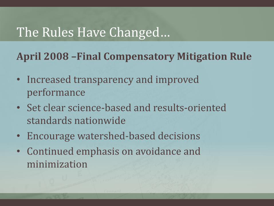
The Rules Have Changed…
April 2008 –Final Compensatory Mitigation Rule
• Increased transparency and improved performance
• Set clear science-based and results-oriented standards nationwide
• Encourage watershed-based decisions
• Continued emphasis on avoidance and minimization
Overview
AASHTO TIG – Environmental Planning GIS Tools
Lead States Team – Texas and Maryland
Texas DOT GIS Screening Tool
Maryland SHA’s Green Infrastructure Assessment and Approach
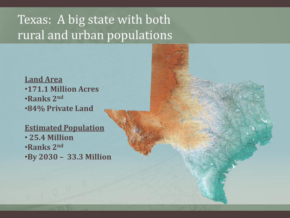
Texas: A big state with bothrural and urban populations
Land Area•171.1 Million Acres•Ranks 2nd
•84% Private Land
Estimated Population• 25.4 Million•Ranks 2nd
•By 2030 – 33.3 Million

Environmental Planning Tools
TxDOT has acquired GIS tools from U.S. EPA:
• Texas Ecological Assessment Protocol (TEAP)
• GIS Screening Tool
• NEPAssist

Composite: identifies important ecological resources in each ecoregion across Texas
What is TEAP?

What is GISST?

GIS-ST Calculation Example
Rank Value
1 < 20% of the grid cell
2 20-29% of the grid cell
3 30-39% of the grid cell
4 40-49% of the grid cell
5 > 50% of the grid cell
% WildlifePercentage of cell that is identified as wildlife habitat In general, a score of “5”
indicates a high degree of concern and a “1” indicates a low degree of concern
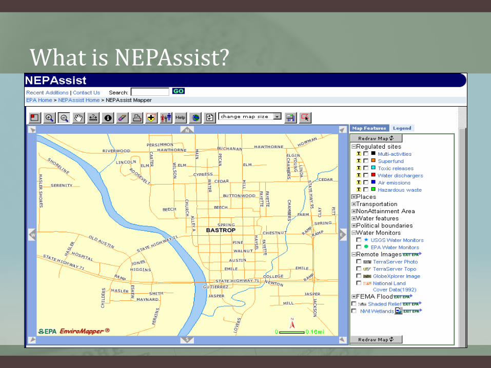
What is NEPAssist?
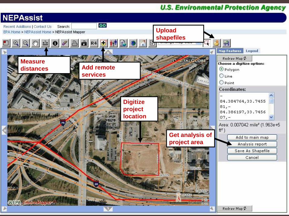
Digitize
project
location
Upload
shapefiles
Get analysis of
project area
Measure
distances Add remote
services
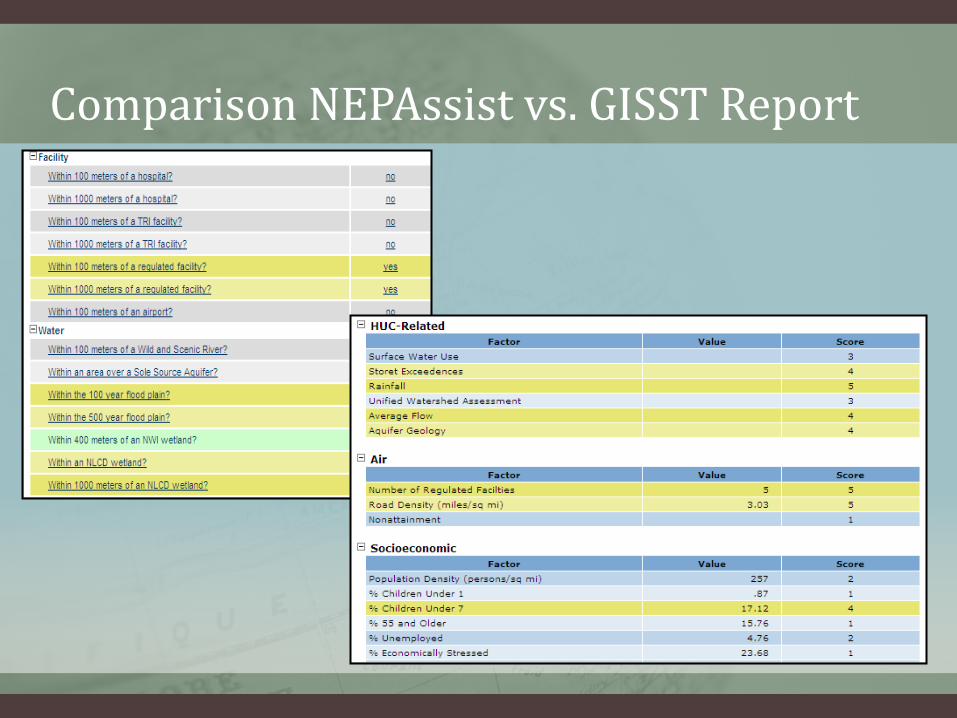
Comparison NEPAssist vs. GISST Report

Alternative 1: GISST ReportDirect Impacts

Alternative 2: GISST ReportDirect Impacts

GISST Database Comparison of AlternativesCorridor Alternative 1 2 3 4 5 6
Number of facilities 5 2 1 4 0 5
score 5 3 2 5 1 5
% Wildlife 79.78 60.92 89.96 86.05 68.01 75.11
5 5 5 5 5 5
% Agriculture 10.05 32.16 3.68 2.56 25.96 15.42
1 3 1 1 2 1
% Wetlands 75.98 59.81 87.17 80.54 67.96 74.88
5 5 5 5 5 5
stream density 2.61 2.71 1.63 3.56 1.69 2.43
5 5 5 5 1 5
% 100 year floodplain 84.9 70.9 88.92 87.17 75.56 84.53
5 5 5 5 5 5
% 500 year floodplain 100 99.99 88.92 100 99.99 99.99
5 5 5 5 5 5
Land Use Ranking 5 4 5 5 4 4

Texas Case Study – Interstate 69 Project
• Planning and Development
• Location
• Environmental Study
• GIS tools used
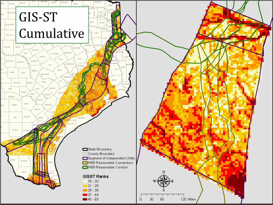
GIS-STCumulative

Current and Future Efforts to Enhance GIS Tools
• Expansion of TEAP to a South Central US Regional Ecological Assessment Protocol (REAP)
• Recalculation to a 0.25 km2 grid—more granular grid for medium size project level analysis
• Recalculations using new land cover data• GISST Incorporation into NEPAssist Website

Maryland: A small state with many people
Land Area• 6.2 Million Acres• Ranks 42nd
• 20.8% developed• 21.9% protected
Population• 5.6 Million• Ranks 19th
• By 2030 – 6.7 Million

Green Infrastructure
“Strategically planned and managed networks of natural
lands, working landscapes and other open spaces that
conserve ecosystem functions, and provide associated benefits to
human populations”
Jane Hawkey, Jane Thomas, IAN Image Library (www.ian.umces.edu/imagelibrary/)

EcologicalFeatures
Large Blocksof Contiguous
Forest
Large Contiguous
Wetland Complexes
RiparianAreas
UniqueWetlandHabitats
SteepSlopes
Waterfowl Concentration
and Staging Areas
Natural Heritage Areas
Existing Protected
AreasRare, Threatened,
and Endangered Species Sites
Habitat Protection
Areas
Colonial Waterbird
Nesting Locations
• Strive to include full range of ecosystem elements vs. single species focus
• Multidisciplinary Effort – DNR biologists – Aquatics,
Forests, Wildlife and Heritage
– Scientific Community
• Limited to features with GIS data available statewide
Maryland’s Green Infrastructure AssessmentSelection of Ecological Components

Maryland’s Green Infrastructure AssessmentComposite of Ecological Features

Green Infrastructure Approach
“… a process that promotes a systematic and strategic approach to land conservation at the
national, state, regional, and local scales encouraging land use planning and practices that
are good for nature and people.”
Mark A. Benedict, Edward T. McMahon, 2006, “Green Infrastructure”

Core
Core
CoreCore
Core
Cores are unfragmented natural
cover with at least 100 acres
of interior conditions.
Core
Core
CoreCore
CoreHub
Hub
Hub
Hubs are groupings of core areas
bounded by major roads or
unsuitable land cover
Corridors link hubs and allow
animal, water, seed and pollen
movement between hubs
The Green Network

GI Gaps – Repairing the Network and Restoring the Chesapeake Bay
• Undeveloped Gaps may be suitable for restoration activities
• Restoration benefits achieved at local and regional scales
• Hub and Corridor rankings can be used to prioritize restoration sites

GREEN INFRASTRUCTURE STRATEGIC APPROACH
US 301 Case Study

US 301 Waldorf Area Transportation Improvements ProjectMaryland State Highway Administration
Partners:

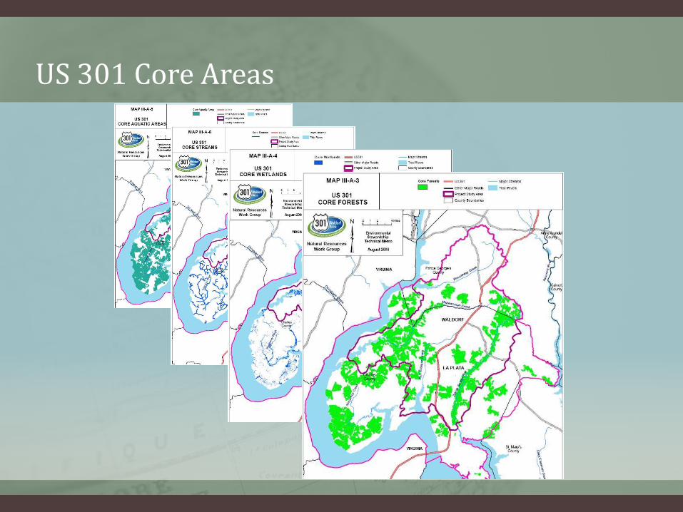
US 301 Core Areas

Scale Variable Scale
weight
Variable weight
within scale
Total weight
Core area/Site Hub area 20.0 0.100 2.0
ESA area 0.100 2.0
Area of mature interior forest 0.100 2.0
Area of unimpacted wetlands 0.100 2.0
Length of core streams 0.100 2.0
Maximum depth of core or site 0.100 2.0
Distance to major roads 0.100 2.0
Distance to development 0.100 2.0
Proximity index 0.100 2.0
Connectivity index 0.100 2.0
Hub ESA area 20.0 0.182 3.6
Area of mature interior forest 0.182 3.6
Area of unimpacted wetlands 0.091 1.8
Length of core streams 0.091 1.8
Maximum depth of hub 0.091 1.8
Distance to major roads 0.091 1.8
Distance to development 0.091 1.8
Proximity index 0.091 1.8
Connectivity index 0.091 1.8
Corridor Average rank of linked hubs 10.0 0.333 3.3
Number of hubs linked 0.333 3.3
Major road crossings without bridges 0.333 3.3
8-digit watershed Anadromous fish spawning habitat use 10.0 0.500 5.0
Percent core streams in watershed 0.500 5.0
12-digit watershed Stronghold watershed (Tier 1/Tier 2/neither) 10.0 0.500 5.0
Mean combined IBI score 0.500 5.0
Grid cell (36 m2) ESA presence and rank 40.0 0.071 2.9
Ecological Community Group rank 0.071 2.9
Forest maturity 0.286 11.4
Wetland condition and proximity 0.143 5.7
Proximity to core streams 0.143 5.7
Proximity to water 0.143 5.7
Distance to edge of forest, wetland, or water 0.143 5.7
Distance to development 0.000 0.0
TOTAL 100.0 100.0
US 301 Project Overall Ecological Score


Hub and Corridor Network Environmental Stewardship Needs
Environmental Stewardship Activities
Conservation / Preservation 60%
Restoration / Creation 18%
Management Actions 11%
Recreation / Public Access to Open Space 11%
Priority Natural Resources
Forests 22%
Streams and Aquatic Resources 19%
Wetlands 17%
Marine Fisheries 10%
Species Habitat 11%
Passive Recreation Areas 5%
Historic/Archeological 6%
Agriculture 9%

US 301 NEXT STEPS
• Field truth opportunities
• Select sites
• Establish protocols for future transportation projects

33
Project Selection Methods
• Government agencies and NGOs typically use a rank-basedapproach to select projects for implementation.
• The rank-based approach focuses only on the benefits of a project without considering the project’s cost, which can result in highly inefficient investments.
• It ignores potential “good buys” that offer high quality (environmental benefits) at a significantly lower cost.
• The use of optimization in project selection provides a means to extend the reach and effectiveness of environmental efforts.

0%
10%
20%
30%
40%
50%
60%
70%
80%
90%
100%
0% 10% 20% 30% 40% 50% 60% 70% 80% 90% 100%
% T
ota
l Acre
s.
% Total Costs
OM
Rank Based
45 degree line
Differences in Selection Models

35
Project Selection Using Optimization
• Optimization Decision Support Tool requirements
– Opportunities (Environmental stewardship projects)
– Benefits (Project benefit scoring/ranking)
– Costs (Financial investment required to achieve benefits)
– Constraints (Budget scenario, other decision constraints)
• Tool benefits
– Easy to use (Excel interface)
– Flexible (answer multiple planning questions)
– Ability to run multiple scenarios (sensitivity analysis)
– Potential to extend limited funds for compensatory mitigation and environmental stewardship

• Compliance with existing regulations
• Defensible decisions
• Accelerated project delivery
• Improved resource protection
• Sustainable planning
• Supports a watershed approach
• Scalable solution
• Can be integrated with existing GIS data
Why Use These Tools?

Why Use These Tools?
Because we can’t afford not to.

Contact Information: Texas Department
of Transportation
Troy Sykes
512-416-2571
Maya Coleman
512-416-2578
Maryland State Highway Administration
Sandy Hertz
410-545-8609
Greg Slater
410-545-0412
U.S. EPA, Region 6
Sharon Osowski
214-665-7506