Development of On-Board Orbit Determination System for Low Earth Orbit (LEO) Satellite Using Global Navigation Satellite System (GNSS) Receiver

Sandip Aghav, S. A. Gangal Department of Electronic Science, University of Pune, Pune Maharashtra, India

1.0 Abstract:

In order to make the orbit control system autonomous, and reduce the need for ground intervention there is a need for an on-board availability of continuous and accurate knowledge of the satellite orbit. In the present work we propose to use on-board GNSS receiver to compute the orbit of the Low Earth Orbit (LEO) satellite. There are six orbital elements defined for a satellite, which are to be specified to define the satellite orbit. With the help of four GPS satellites in the GNSS constellation, on-board Global navigation Satellite System (GNSS) receiver collects the navigational data and calculates its own position. The position information in the GNSS contains the GNSS data in the form of Pseudo-ranges with respect to time. From this information; position and velocity vector is calculated as a function of time. Orbital elements of the current position are calculated using the position and velocity vectors. Comparing theses orbital elements with the reference orbit, one can get the errors out of that and correct it further. Measurement noise and process noise models are selected for simulating actual scenario. For orbit estimation, Extended Kalman filter method is used. Runge-Kutta method is used to propagate the reference orbit. Software for the orbit integration is developed in MATLAB. The effect of various zonal perturbations like J2, J3, and J4 were tested. From this study it is observed that J2

is the main zonal parameter which affects the state vector more. However j3 and j4 terms are included, the effect shows more deflections. Parameters J3, and J4

affect for long term integration. In the present application long term integration is not used. Equation of motion with J2 only is used for orbit integration. The state transition matrix is used to propagate covariance matrix. It is observed from that, orbit of the satellite is confined with its orbital plane but when secular perturbation term j2 is introduced, the satellite orbit gets affected due to gravitation pull up because of earth obletness. Normally distributed random noise vectors are generated. These vectors are further used to simulate GPS measurements. The main purpose of this work is to study a rather simple but still fairly accurate algorithm to determine the artificial satellite orbit, in its real time and with low computational burden, by using raw navigation solution provided by GPS receiver

2.0 Introduction:

GNSS (Global Navigation Satellite System) is a satellite system which is used to pinpoint the geographic location of a user's receiver anywhere in the world. Two GNSS systems are currently in operation: the United States' Global Positioning System (GPS) and the Russian Federation's Global Orbiting Navigation Satellite System (GLONASS). For the present application, well established Global Positioning System (GPS) is used. This determines the position, velocity and time (PVT) with high precision. The GPS system allows GPS receiver to determine its position and time at any place using data signal from at least four GPS satellites [1]. Using such system, it is proposed to compute, in near real time, a state vector composed of position, velocity, GPS receiver clock bias and drift of a satellite equipped with on-board GPS receiver. This can be done by filtering the raw navigation solution provided by the receiver. Kalman Filter is used to estimate the state vector based on such incoming observations from the receiver. The filter dynamic model includes geopotential (i.e. J2, J3 J4 ) solar radiation pressure, and the perturbation due to the Sun and the Moon and the clock bias is modelled as a random walk process. The observations includes the raw navigation data composed of position and time bias that are computed stepwise by GPS receiver and provides instantaneously the absolute position.

3.0 Methodology:

The orbit determination algorithm for the on-board orbit determination is developed. In the present work, the Extended Kalman filter is selected to generate the state estimates of the satellite orbit. The dynamic model of the satellite orbit is designed and simulated. The perturbations like j2, J3 and j4 are considered for simulations. The calculations of Jacobian matrix, state transition matrix are also carried out. The sample raw navigation data is processed and position of the GPS satellite is also calculated.

3.0.1 Extended Kalman Filter (EKF) Algorithm: Theoretical Background: Equation of motion for satellite orbit is of non-linear form, and therefore EKF is selected for orbit estimation. It can be considered as two step procedure; the first being the time updates which predicts the state vector at subsequent time using the system dynamic model. Second step is measurement update that estimate the state vector at the current time based on the measurement and the prior information from the first step.

System model and measurement model are respectively[2]

)()),(( twttf xx

(1)

2,1))(( kthz kkkk x (2)

3.0.1.1 Time update:

In the time update step of an EKF, is further divided into two parts, state vector and state error covariance matrix update with time. In this step, the state vector and state error covariance matrix are propagated for the fixed time interval.

)(x t =[x y z vx vy vz], a priori state estimate. Where T is the time interval between measurement (i.e tk-tk-1), and

11 ˆ

1

),(

kk xtxk

kkk tx

ttxftF (3)

where 1ktF is a Jacobian matrix of the system dynamic equation and )(tw is a process noise.

3.0.1.1.1 State vector update:

Equation of motion of pure Keplerian orbit is given by;

3 rr

r

(4)

Where ‘r’ is the distance between satellite to centre of the Earth and

is the Gravitational constant.

Equation of motion is second order differential equations of the form;

dt

drrt

dt

rd,,

2

2

;

Using 4th order Runge-Kutta method, position and velocity vectors as a function of time is calculated by integrating the acceleration components; Velocity vector is (t)k v (t)j v (t)i v v(t) zyx

and

position vector is r(t) = rx(t)i + ry(t)j + rz(t)k

Their magnitudes are given by;

22y

2 vvv)( zxtv

and 22y

2r)( zx rrtr

The x, y and z components of Equation of motion (Eqn. 4) with term J2 are given by,

152

31

2

22

23 r

z

r

RJ

r

xx e (4a)

xx

yy

(4b)

Ttkkk 11, FI

2

22

2353

2

31

r

z

r

RJ

r

zz e

(4c)

To update the state vector, equation 4a, 4b and 4c are numerically integrated using Runge-Kutta 4th order fixed step size method.

3.0.1.1.2 State Error Covariance Matrix update:

The State Error Covariance Matrix is propagated using following equation,

11,11,1/ QPP kT

kkkkkkk (5)

Where 1,kk is the transition

matrix approximation, which is computed using a first-order Taylor series expansion:

1Pk is a priori State Error Covariance Matrix

1/P kk is updated/predicted state error covariance matrix, 1Qk process noise covariance matrix.

3.0.1.2 Measurement update:

In this state, the actual measurements are collected from measuring instrument and modelled in measurement model given by;

2,1))(( kthz kkkk x (6)

The measurement matrix for the same is calculated from relation[2],

1k/kk x̂txk

kkkk tx

t),t(xhH

(7)

kH is measurement information matrix. With abovementioned parameters Kalman Gain Kk is calculated using the relation

1

kTk1k/kk

Tk1k/kk RHPHHPK

The Kalman Gain Kk is used as feedback for correcting state estimates, kR is measurement noise covariance noise matrix and new estimate ( kx̂ ) is obtained from equation given below;

START

ACQUIRE A PRIORI STATE AND COVARIANCE ESTIMATES AT t0 SET k=0, i.e Initialization

k=k+1 ACQUIRE A MEMBER OF OBSERVATION VECTOR

Y

PROPAGATE STATE VECTOR TO tk, CALCULATE STATE TRANSITION MATRIX F (tk, tk+1)

CALCULATE EXPEXTED MEASUREMENT Xk AND PARTIAL DERIVATIVES OF Xk WITH RESPECT TO

Xk-1(tk)

PROPAGATE STATE NOISE COVARIANCE MATRIX Q(tk, t )

PROPAGATE ERROR COVARIANCE MATRIX Pk-1(tk)

CALCULATE GAIN MATRIX K

UPDATE X*k-1 TO BECOME kth STATE ESTIMATE

UPDATE ERROR COVARIANCE MATRIX Pk

PROPAGATE Xk(tk) TO ANY TIME OF THE INTREST

LAST OBSERVATION ?

END

Y

N

khz kkkkk ,x̂Kx̂ 1/

And new predicted error covariance ( kP ) is obtained from equation given below;

Tkkk

Tkkkkkkk KRKHKIPHKIP 1/

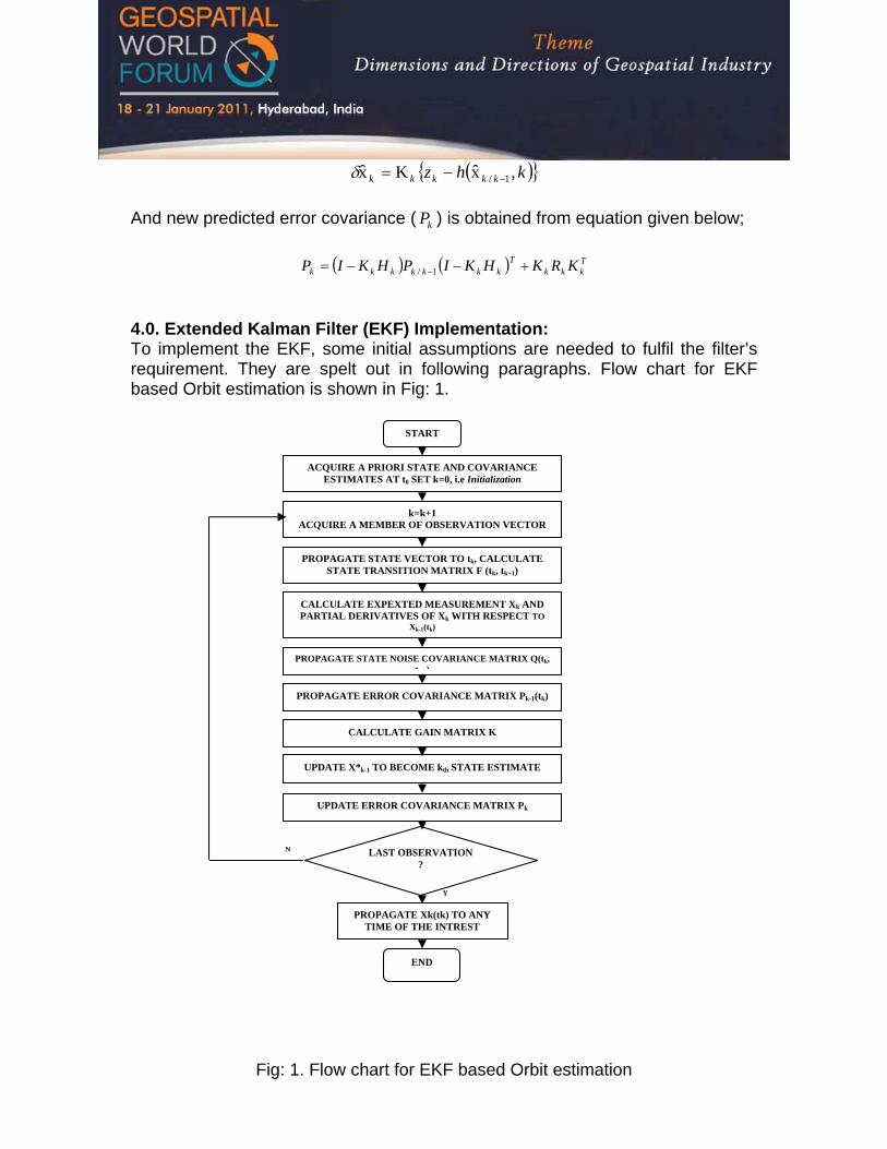
4.0. Extended Kalman Filter (EKF) Implementation: To implement the EKF, some initial assumptions are needed to fulfil the filter’s requirement. They are spelt out in following paragraphs. Flow chart for EKF based Orbit estimation is shown in Fig: 1.

Fig: 1. Flow chart for EKF based Orbit estimation

4.0.1. Initialization: For the system state vector propagation, the system model (i.e. equation 1a) is numerically integrated using Runge-Kutta 4th Order method. To start the Kalman filter, it requires initial state estimate and initial state error covariance matrix. The state vector ( )(x t ) of the system model is given by;

)(x t =[x y z vx vy vz]6x1 ;

These include the six dimensional satellite position and velocity vector, the three dimensional. The filter is started using the receiver internal single-point navigation solution. Furthermore, a diagonal apriori covariance matrix 1Pk with standard deviations (s ) of 10 m (position), 0.1 m/s (velocity), is assumed. With these assumptions the apriori covariance matrix 1Pk is given by;

1Pk =diag [sx2 s y

2 s z2 s vx

2 s vy2 s vz

2]6x6;

Within the time-update phase of the EKF, the satellite state vector is numerically propagated from the latest state estimate, while the remaining parameters are assumed to be constant between the epoch’s ti-1 and ti.

4.0.2. Propagation of State and State Error Covariance matrix:

The state transition matrix (F ) is used to propagate covariance matrix is given by,

Ttkkk 11, FI

Where,

663333

33331 0

0

XXX

XXk J

ItF

(8)

(9)

Where, J [3] is Jacobian coefficient.

35255

53525

55352

333

333

333

rrzzyrzxr

yzrrryyxr

xzrxyrrrx

J

To cope with deficiencies of the employed propagation model, a fixed diagonal process noise matrix 1Qk is considered in the time update of the covariance matrix.

11,11,1/ QPP kT

kkkkkkk

Representative process noise values used in the practical applications are (10- 3m)2 (position), (10- 6 m/s)2 (Velocity). With these settings, the Kalman filter” memory” is dominated by the acceleration process noise, which reflects the expected uncertainty of the dynamical model.

5.0 GPS data processing:

There are two types of GPS codes are transmitted by the GPS satellite vehicle. One of them (P-code) provides precise positioning with an accuracy of approximately tens of meters. This code can only be used by a receiver with access to the encryption key. This code is only for military users. The second code is available to any commercial user. This code is known as Coarse/Acquisition (C/A) code and this code is discussed in this overview. Each satellite transmits two carrier signals. One is centred at 1575. 42 MHz (known as L1 carrier) uses Phase Shift keying (PSK) to modulate both C/A and P-code onto the carrier. The other signal (known as the L2 carrier) is centred at 1227.60 MHz and uses PSK to modulate P-code onto the carrier. L1 carrier is the signal used by the commercial receivers. It is modulated with 1.023 MHz Pseudo-Random noise (PRN) code which is unique to each satellite. Each GPS satellite transmits the Navigation Message through C/A code. The C/A codes from at least four GPS satellites are required to calculate the user receiver position in Earth Centred Earth Fixed (ECEF) coordinate system [4].

5.0.1 GPS Navigation Solution:

It is stated earlier that minimum four GPS satellite are must be in view for the receiver to determine to 3-dimentional position. This is because there are four unknowns in the set of four navigation equations. Therefore, to solve for user position and time, we need to solve the following simultaneous equations.

tczZyYxX .)()()( 21

21

211

(10a)

tczZyYxX .)()()( 22

22

222

(10b)

tczZyYxX .)()()( 23

23

233

(10c)

tczZyYxX .)()()( 24

24

244

(10d)

4321 ,,,

; are the pseudo-ranges to each of the satellites. A pseudo-range is

a measurement of the distance between the satellite and the receiver.

iii ZYX ,, ; for i=1,2,3,4 are the coordinates of the satellites in the Earth Centred Earth Fixed, WGS-84 coordinate reference frame,

x, y z are the receiver WGS-84 coordinates,

c=2.288*10+08 (speed of light) m/s

t is the receiver clock offset from GPS time (satellite time)

By linearzing equations 10a, 10b, 10c and 10d , one can get the observation vector (i.e. receiver position x, y, z ) and clock bias t.

GPS satellite sends data through navigation message in frames to GPS receiver to in solving above mentioned simultaneous equations. These data are in spherical coordinates and required to transformed into Cartesian ones.

5.0.2 GPS satellite Navigation message:

The navigation message includes Almanac data, ephemeris data, timing data, ionospheric delay data and health data of the satellite. The information in the navigation message has basic five frames. Each frame is subdivided into five 300-bit sub-frames and has 10 words of 30 bit. Out of above mentioned frames, the Satellite Ephemeris data, ionospheric data frame and satellite timing data frame are of interest for the present work. A detailed description of all information contained in the navigation message is beyond the scope of this text. The sub-frame of navigation message contains the ephemeris data, which is used to determine the precise satellite position and velocity required by the navigation solution. This ephemeris data is valid over a relatively short period of time (several ours), and applies only to the satellite transmitting it. The components of the ephemeris data [5] are listed in table 1.

Table: 1 Components of Ephemeris data

Name Description Units M0 Mean anomaly at reference time semicircle

n Mean motion difference from computed value semicircle/s e Eccentricity dimensionless

a Square root of semimajor axis 2/1m

0

Longitude of ascending node of orbital plane at weekly epoch

semicircle

0i Inclination angle at reference time semicircle

Argument of perigee semicircle

Rate of right ascension semicircle/s IDOT Rate of inclination angle semicircle/s

ucC Amplitude of the cosine harmonic correction term of the argument of the latitude

rad

usC Amplitude of the cosine harmonic correction term of the argument of the latitude

rad

rcC Amplitude of the cosine harmonic correction term of the orbit radius

m

rsC Amplitude of the sine harmonic correction term of the orbit radius

m

icC Amplitude of the cosine harmonic correction term of the angle of inclination

m

isC Amplitude of the cosine harmonic correction term of the angle of inclination

rad

et0 Ephemeris reference time s

IODE Issue of data, ephemeris dimensionless

5.0.2 Calculation of ECEF coordinates of the GPS satellite from Ephemeris data:

As shown in Table: 1, the ephemeris data will be extracted from navigation message and then further used to compute the GPS satellite position in the form of Earth Centred Earth Fixed (ECEF) coordinate frame using following algorithm[5].

2)( aa

; Semimajor axis (11)

30 / an ; Computed mean motion, rad/s (12)

kkk EeEM sin ; Kepler’s equation of eccentric anomaly (13)

k

kk Ee

Ef

cos1

1coscos 1 ; True anomaly from cosine (14)

k

kk fe

feE

cos1

coscos 1 ; Eccentric anomaly from cosine (15)

Accordingly, the second harmonics terms of the various quantities are also determined. With the help of above mentioned algorithm the GPS satellite position in ECEF coordinate frame is determined using equations.

kkkkk iyxX sincoscos ; ECEF X coordinate (16)

kkkkk iyxY coscoscos ; ECEF Y coordinate (17)

kk iyZ sin ; ECEF Z coordinate (18)

The software for the same is developed in MATLAB.

6.0. Results and discussion:

In this section, the results of Time Update Step of Kalman filter and GPS data processing are given.

6.0.1. State Vector Propagation:

As shown in the fig. 2 pure Keplerian Orbit is integrated for a period of T=86,400 sec. Step size t =10 sec is selected for orbit integration. State vector used for orbit integration is propagated using following initial conditions,

r0= [5492.00034; 3984.00140; 2.95581]; v0= [-3.931046491; 5.498676921; 3.665980697];

It is observed from fig.2 that, orbit of the satellite is confined with its orbital plane i.e. central gravitational field. The equation of motion is integrated with J2.

The equations given in 4a, 4b, and 4c are integrated to get the J2 perturbed orbit. As can be seen from fig 3 when secular perturbation term J2 is introduced, the satellite orbit gets deviated from it central gravitation field. The main deviation from central gravitational field is caused by dynamic flattening of the earth. In the Geodetic Reference System 1980 (GRS80), normal field of the flattening coefficient is represented by term J2= 0.001082. Similarly J2 and J3 are given as, J3= -0.0000025323 and J4= -0.0000016204. After adding J3 and J4 terms, the orbit shows additional deviation as shown in fig. 4. Normally distributed random noise vector are generated. They are further used as GPS measurements. Fig.5. shows the noise distribution of the GPS measurements over a period of time

(T=86,400 sec). The standard deviation s

= 100m in position vector of GPS

measurement is assumed.

-1-0.5

00.5

1

x 104

-1

-0.5

0

0.5

1

x 104

-4000

-2000

0

2000

4000

x[Km]y[Km]

z[km

]

-1-0.5

00.5

1

x 104

-1

-0.5

0

0.5

1

x 104

-4000

-2000

0

2000

4000

x[Km]y[Km]z[

km]

Fig: 2. Pure Keplerian Orbit Integration Fig: 3. Orbit Integration with J2

-1-0.5

00.5

1

x 104

-1

-0.5

0

0.5

1

x 104

-4000

-2000

0

2000

4000

x[Km]y[Km]

z[km

]

0 1000 2000 3000 4000 5000 6000 7000-2

0

2

tsec

rx i

n K

m

Time Vs rxnoise

0 1000 2000 3000 4000 5000 6000 7000-2

0

2

tsec

ry i

n K

m

Time Vs rynoise

0 1000 2000 3000 4000 5000 6000 7000-2

0

2

tsec

rz in

Km

Time Vs rznoise

Fig: 4. Orbit Integration J2, J3 and J4 Fig: 5. Simulated normally distributed noise vector

Fig: 6: Orbital elements in Pure Keplerian Orbit

0 2 4 6 8 10

x 104

6828.951

6828.952

6828.953

6828.954

6828.955

6828.956

tsec

Sem

i-maj

or a

xis(

a) in

Km

Time Vs Semi-major axis

0 2 4 6 8 10

x 104

9.0146

9.0148

9.015

9.0152

9.0154

9.0156x 10

-3

tsec

ecce

ntric

ity(e

)

eccentricity Vs Time

0 2 4 6 8 10

x 104

28.474

28.474

28.474

28.474

28.474

28.474

28.474

28.474

28.474

28.474

tsec

Incl

inat

ion

Ang

le(i)

in d

egre

es

Time Vs Inclination Angle

0 2 4 6 8 10

x 104

35.9118

35.9118

35.9118

35.9118

35.9118

35.9118

35.9118

35.9118

35.9118

35.9118

tsec

Rig

ht A

ssen

tion

of A

scen

ding

Nod

e(O

MG

) in

deg

rees Right Assention of Ascending Node Vs Time

0 2 4 6 8 10

x 104

-44.572

-44.57

-44.568

-44.566

-44.564

-44.562

-44.56

-44.558

-44.556

tsec

Arg

umen

t of

per

igee

(om

g) in

deg

rees

Argument of perigee Vs Time

0 2 4 6 8 10

x 104

0

20

40

60

80

100

120

140

160

180

tsec

Tru

e A

nom

oly(

v) in

deg

rees

True Anomoly Vs Time

Fig: 7. Perturbation of the Orbital elements due to main harmonic J2.

0 2 4 6 8 10

x 104

6810

6820

6830

6840

6850

6860

6870

6880

tsec

Sem

i-maj

or a

xis(

a) in

Km

Time Vs Semi-major axis

0 2 4 6 8 10

x 104

0

0.01

0.02

0.03

0.04

0.05

0.06

0.07

tsec

ecce

ntric

ity(e

)

eccentricity Vs Time

0 2 4 6 8 10

x 104

28.35

28.4

28.45

28.5

28.55

28.6

tsec

Incl

inat

ion

Ang

le(i)

in d

egre

es

Time Vs Inclination Angle

0 2 4 6 8 10

x 104

29

30

31

32

33

34

35

36

tsec

Rig

ht A

ssen

tion

of A

scen

ding

Nod

e(O

MG

) in

deg

rees Right Assention of Ascending Node Vs Time

0 2 4 6 8 10

x 104

-50

-40

-30

-20

-10

0

tsec

Arg

umen

t of

per

igee

(om

g) in

deg

rees

Argument of perigee Vs Time

0 2 4 6 8 10

x 104

0

20

40

60

80

100

120

140

160

180

tsec

Tru

e A

nom

oly(

v) in

deg

rees

True Anomoly Vs Time

Fig: 8. Perturbation of the Orbital elements due to main harmonic J2 J3 and J4.

In Fig: 6, it shows the orbital elements in case of pure Keplerian orbits. In case of pure Keplerian orbit, Earth is assumed to be a spherical, so the only central gravitation force play vital role in orbit integration. From fig.6 it observed

0 2 4 6 8 10

x 104

6824

6825

6826

6827

6828

6829

tsec

Sem

i-maj

or a

xis(

a) in

Km

Time Vs Semi-major axis

0 2 4 6 8 10

x 104

7

7.5

8

8.5

9

9.5x 10

-3

tsec

ecce

ntric

ity(e

)

eccentricity Vs Time

0 2 4 6 8 10

x 104

28.435

28.44

28.445

28.45

28.455

28.46

28.465

28.47

28.475

tsec

Incl

inat

ion

Ang

le(i)

in d

egre

es

Time Vs Inclination Angle

0 2 4 6 8 10

x 104

28

29

30

31

32

33

34

35

36

tsec

Rig

ht A

ssen

tion

of A

scen

ding

Nod

e(O

MG

) in

deg

rees Right Assention of Ascending Node Vs Time

0 2 4 6 8 10

x 104

-60

-55

-50

-45

-40

-35

-30

tsec

Arg

umen

t of

per

igee

(om

g) in

deg

rees

Argument of perigee Vs Time

0 2 4 6 8 10

x 104

0

20

40

60

80

100

120

140

160

180

tsec

Tru

e A

nom

oly(

v) in

deg

rees

True Anomoly Vs Time

that, the orbital elements are constant except true anomaly ( ), because there is no other force which causes the change in orbital elements. The obtained orbital elements are given below;

Table :2. Variations in orbital elements in different cases.

Orbital Elements

Pure Keplerian Orbit

J2

J2, J3, J4

Max

Min

Max

Min

Max

Min

aKm

6828.956 6828.952

6828.975

6824.416

6871.082

6818.754

e 0.009016 0.009015

0.009311

0.00711 0.064504

0.007943

Ideg

28.47401 28.47401

28.47404

28.43975

28.5831 28.39334

OMGdeg

35.91182 35.91182

35.91182

28.96786

35.92338

29.04105

omgdeg

-44.5593 -44.5708 -32.5345 -58.0807 -0.00189 -46.7252

Variations in the orbital elements due to secular perturbations are shown in Fig. 7 and Fig: 8. Table: 2 also shows the variations in orbital elements produced in different cases.. Equation of the satellite is integrated for period T=86,400 sec with fixed step size=10 sec. As shown in Fig: 7, regression of the ascending node under the J2 perturbation is observed. In case of J2 perturbed orbit, the ascending node and argument of perigee exhibits significant linear variation. The maximum and minimum values are given in Table: 2. The motion of the ascending node occurs because of the added attraction of the Earth’s equatorial bulge, which introduces force components towards the equator. The ascending node regresses for direct orbits (0 deg < i < 90 deg) and advances for retrograde orbits (90 deg < i < 180 deg).

Software for the orbit integration is developed in MATLAB. The effect of various zonal perturbations like J2, J3, and J4 were tested. From this study it is observed that J2 is the main zonal parameter which affects the state vector more. Other parameters like J3, and J4 are affects for long term integration. In the present application long term integration is not required. In this case equation of motion with J2 is used for orbit integration.

6.0.2. State Error Covariance Propagation: To execute this step, a diagonal priori state error covariance is assumed

as follows;

1.000000

01.00000

001.0000

0001000

0000100

0000010

0P

Where sposition= 10m and svelocity= 0.1 m/s

Updated State Error Covariance Matrix is given by,

11,11,1/ QPP kT

kkkkkkk

and tF

kkkke )(

1,1/

With reference to initial conditions, Jacobian Matrix is calculated for single step. The results are given below;

00006-1.28E-10-9.79E09-1.35E

00010-9.79E08-4.39E06-1.82E

00009-1.35E06-1.82E06-1.23E

100000

010000

001000

1/ kkF

And State Transition Matrix is calculated for the same conditions, the result of the same is given below;

0.99999910-4.90E10-6.75E06-1.28E-10-9.79E09-1.35E

10-6.75E107-9.10E10-9.79E08-4.39E06-1.82E

10-6.75E07-9.10E1.00000109-1.35E06-1.82E06-1.23E

110-1.63E10-2.25E0.99999910-4.90E10-2.25E

10-1.63E107-3.03E10-4.90E107-9.10E

10-2.25E07-3.03E110-6.75E07-9.10E1.000001

1/ kk

Similarly from state transition matrix, new updated state error covariance matrix is calculated. With these calculation, the work related to Time update step of the Kalman Filter is completed.

6.0.3 GPS data processing: The software code for the calculation of GPS satellite position in ECEF coordinate system from navigation message is developed in MATLAB environment. The ECEF coordinate for one the sample ephemeris are computed and the value of the same are given below.

X = 10398396.34918728800; Y = -23799638.49937681100; Z = 4116898.20773698440;

Above results are validated with sample data.

Conclusion:

In this work, the Extended Kalman Filter (EKF) algorithm is developed and some part of it is implemented and tested. The state vector is propagated using fixed step size orbit integration. Satellite orbit dynamic model with J2 J3 and J4 are integrated. With this experiment, it is observed that orbit integration with J2 only is

sufficient to use for present application. The state transition matrix of the pure Keplerian Equations is also computed. The ECEF position is calculated by processing GPS navigation message data. With this work, we concluded that for near real time orbit determination applications, the use of simplified dynamic model with J2 perturbation and suitable orbit integration technique reduces computational burden from the hardware.

Acknowledgement: The authors thank the Indian Space Research Organization-University of Pune Space Technology Cell, Pune for the financial support. The authors also thank Dr. Pramod kale

References:

[1] Parkinson B. W, Spilker Jr. “Global Positioning System: theory and Applications”, AIAA, Vol.1, 1996 (Progress in Astronautics and Aeronautica 163).

[2] Fundamentals of Kalman Filtering: A Practical Approach, Second Edition, by Paul Zarchan , AIAA, 2005.

[3] Real time multisatellite orbit determination for constellation maintenance, Proceedings of COBEM 2007.

[4] NAVSTAR GPS user equipment introduction, US Government, chapter 7. [5] Global Positioning System, Inertial Navigation and Integration, Mohinder

Grewal, A John Wiley and Sons Inc, Publication, page.no 37.

Paper Reference No.: PN-288

Title of the paper : Development of On-board orbit determination system for Low Earth Orbit (LEO) satellite Using Global Navigation Satellite System (GNSS) Receiver

Name of the Presenter: Mr. Sandip Aghav

Author (s) Affiliation: Senior Research Fellow and PhD Candidate

Mailing Address: Department of Electronic Science, University of Pune, Maharashtra, India 411 007

Email Address: sandip.aqua@gmail.com

Telephone number (s) : 020-25699841, Mobile no.: +919689423702

Fax number (s) : 020-25699841

Bio-data

i) Presently working as a Senior Research Fellow (SRF) and a PhD student in the Department of Electronic Science, University of Pune on project “Autonomous Satellite Navigation System for Low Earth Orbit (LEO) satellite using Global Navigation Satellite (GNSS)” funded by Indian Space Research Organization (ISRO).

ii) Worked as a Junior Research Fellow (JRF) in the Department of Electronic Science, University of Pune on project “ Development of Ground Station for ANUSAT” funded by Indian Space Research Organization (ISRO).

iii) Post Graduated from Department of Electronic Science, University of Pune in MSc. with Electronic Science as a Special subject.