State of CaliforniaThe Resources .Agency

DF.PARTMENT OF WATER RESOURCESNorthern District

SAN JOAQUIN RIVER TRIBUTARIES

SPAWNING GRAVEL ASSESSMENT

STANISLAUS, TUOLUMNE, MERCED RIVERS

t

NOVEMBER 1994

C--1 0471 3C-104713

SAN JOAQUIN RIVER TRIBUTARIES

SPAWNING GRAVEL ASSESSMENT

STANISLAUS, TUOLUMNE, AND MERCED RIVERS

TABLE OF CONTENTS

FOREWORD .......................................................... iiiMETRIC CONVERSIONS ..............................................back cover

PART I: INTRODUCTION

PURPOSE AND SCOPE ..............................................1REPORT ORGANIZATION ...........................................1PREVIOUS STUDmS ................................................ 4SUMMARY, CONCLUSIONS AND RECOMMENDATIONS ...............4

PART II: CHINOOK SALMON AND SPAWNING GRAVEL

CHINOOK SALMON AND SPAWNING GRAVEL ........................6The Redd .................................................... 7Redd Location ................................................ 8Incubation and Emergence .....................................10

DISCUSSION OF SPAWNING GRAVEL SUITABILITY ..................10Grading of Gravel for Suitability Analysis ........................10Synopses of Spawning Gravel Suitability Investigations .............11

PART III: SPAWNING GRAVEL SAMPLING METHODOLOGY

INT--RODUCrION ...................................................14 -BULK SAMPLING ..................................................14

" Sample Location Seloztion .....................................16Sample Quantity .............................................16Mechanical Analysis ..........................................16Mechanical Analysis Graphs ...................................18

SURFACE SAMPLING ..............................................19PREFERRED SPAWN~G GRAVEL AREA MEASUREMENT .............21

PART IV: SPAWNING GRAVEL RESOURCE ASSESSMEN~r

BULK SAMPLING DATA ANALYSIS .................................. 22SURFACE SAMPLING DATA ANALYSIS 25ANALYSIS OF SPAWNING GRAVEL AREA ............................25

C--1 0471 4C-104714

PART V: RIVER CONDITIONS

VEGETATION ENCROACHMENT .....................................30COARSE GRAVEL DOWNSTREAM OF DAMS .........................30ENGINEERED RIFFLES ON THE TUOLUMNE RIVER ....................31

REFERENCES

References Cited ..................................................... 32

LIST OF TABLES

I. Suitable Salmon Spawning Grovel for Chinook Salmon .................12II. Field and Laboratory Sieve Sizes ...................................18III. Comparison of D~o and D2o Sizes for Substrate Grovel ..................23IV. Means and Variances of D~0 and D20 Fractions ........................24V. Sand Laden Riffles ...............................................24VI. Preferred Spawning Gravel Area, Stanislaus River .....................27VII. Preferred Spawning Gravel Area, Tuolunme River .....................28VIII. Preferred Spawning Gravel Area, Merced River .......................29

LIST OF FIGURES

1. Study Area Location Map ............................................22. Study Reaches with Selected River Miles or Riffle Numbers ...............33. River Grovel Bed Depicting Surface and Substrate Layers .................74. Profile and Top View of a Salmon Redd ................................85. Longitudinal Sections of a Spawning Area .............................96. Relationship between Embryo Survival and Dg/De Ratio ..................I 17. Fine Sediment versus Fry Emergence 138. Bulk Sample Size Standards 179. Mechanical Analysis Graph ..........................................20

LIST OFAPPENDICES

Appendix A -- Gradation CurvesAppendix B -- Bulk Sampling Data, CombinedAppendix C -- Bulk Sampling Data, Surface and SubstrateAppendix D -- Wolman CurvesAppendix E -- Selected Riffle Maps, Tuolun’me River

C--1 0471 5C-104715

FOREWORD

The Stanislaus, Tuolumne and Merced Rivers support a natural run of chinook salmon which return fromthe Pacific Ocean via San Francisco Bay, the Sacramento/San Joaquin Delta and the San Joaquin River.Since the 1940s, Chinook salmon production has declined by over 85 percent in the San Joaquin Riverdrainage (Low, 1993).

In 1988, with the passage of the Salmon, Steelhead, Trout and Anadromous Fisheries Program Act, theCalifornia Legislature mandated that the Department of Fish and Game (DFG) restore depleted salmon,steelhead, trout and anadromous fish stocks statewide. The Legislature decreed that the policy of the Stateis to increase the natural production of salmon and steeLhead trout by the end of the twentieth century. TheLegislature thereby directed that the DFG develop a plan and a program to double the current naturalproduction of salmon and steelhead resources (Low, 1993).

Restoration of salmon spawning and rearing habitat is a major part of the DFG program. A critical factoraffecting the development and survival of salmonid eggs and alevins is size distribution of spawninggravel. The distribution of spawning gravel in the San Joaquin River tributaries is altered by dams,strearnflow diversions, and mining. Dams eliminate both the delivery of spawning-size gravel fromupstream sources and the necessary high flows which flush clogging sediments from spawning areas.Diversions and low flows have caused formation of sandbars which reduce available spawning area.Aggregate mining, instream and offstream, have locally eliminated suitable spawning gravel from thechannel (Low, 1993).

I11

C--1 0471 6(3-104716

PART I: INTRODUCTION

PURPOSE AND SCOPE

This report documents the spawning gravel quality and quantity in the lower Stanislaus,Tuolumne and Merced Rivers, about 55 river miles of the San Joaquin basin. The study areasand surrounding cities are shown in Figure 1. Figure 2 shows the study reaches of each river.The study reaches are:

¯ Lower Stanislaus River from Goodwin Dam to Riverbank.¯ Lower Tuolumne River from La Grange Dam to Waterford.¯ Lower Merced River from Crocker-Huffman Dam to Cressey.

The reaches range from approximately 20 to 25 miles in length. They begin immediatelydownstream of large dams where the rivers emerge from Sierra Nevada foothills onto the Sanloaquin Valley floor. In the foothills, the rivers flow through steep-walled canyons incised intouplifted volcanic, sedimentary or metamorphic rocks. Where these rivers empt3, onto the valleymarks a gradient inflection from relatively steep gradients in the foothills to gentle gradients onthe valley floor.

Riffles and river miles, such as those in Figure 2, are plotted in detailed fiver atlases by theDepartment of Fish and Game. The riffle or river mile numbers plotted in Figure 2 are selectedas general reference points. Riffle numbers are plotted on the Merced River map in lieu of rivermiles.

Field work consisted of bulk and surface gravel sampling and spawning gravel areameasurement. Bulk gravel samples were taken at 51 salmon spawning fifties. Surface sampleswere taken at 59 riffles.

Bulk and surface sampling data are statistically reduced to represent surface and substrate sizecomposition. Size composition is presented as percent by weight which is customary inspawning gravel assessment (Young et al, 1991).

Spawning gravel area is measured in square feet. The measurements were performed at fiftieswith preferred spawning areas during typically available spawning flows.

REPORT ORGANIZATION

Part II of this memorandum discusses factors pertinent to spawning gravel. A discussion of fieldsampling methodology and gravel resource assessment is in Part III. Part IV provides anassessment of the spawning gravel resources on the three study reaches. Part V is a description

1

C--1 0471 7C-104717

Figur~ t

\.

z’ <~~%~’~1’

SCALE IN MILES~i=’9i " ....." LEGEN D

~ Study ReQch

County BoundoriesOakda|e Raser~oir

~ RiverMODESTO

Lak$

..,..-,’"

THE RESOURCES AGENCYDEPARTMENT OF" WATER RESOURCES

NOR’IHERN DIS’I~ICT

San dooquin River TributariesSpawnin9 Grc~vel Assessment

Lower Stonislaus, Tuolumne and Merced Rivers

STUDY AREA LOCATION MAP

C--1 0471 8C-104718

SiGn isl cu s River: Good win.~.Fe#yK"~g~t~D-’cm, d~D°m/t°G°°~w~"R iverb cn k

~:

~RM4~

R~40

5~ ~ ~ LEGEND

~ . ’. Riverbank ~ River withi Mile Loc~tlons~.~ or Riffle Locotion

River Mile or~ Tuolumne River: Lo Grange Dam to Woterford~, : RM= River Mile

~ .~ R= Riffle

~ Lo GronqeRMSO ~ Dora

Waterfor~ ge

Merced River: Crocker- Huffmon Dam to CresseyCrocker --

~ ffman Dam

~ R22

[ ’ -Cressey

D~R~ OF WA~ R~RC~

San goaquin River TributariesSpewning Oreve! Assessment

Lower Stonislous, Tuolumne and Merced Rivers

STUDY REACHES WITH SELECTEDRIVER MILES OR RIFFLE NUMBER~

C--1 0471 9C-104719

of fiver conditions. Mechanical gradation curves, Wolman cun, es, and raw-data spreadsheetsare contained in Appendices A,B,C and D. Appendix E contains maps of selected fifties on theTuolumne River

PREVIOUS STUDIES

The Department of Water Resources has participated in enhancement projects on the SanJoaquin tributaries as mitigation for the Four Pumps Agreement (Landis, 1993). The sites whichhave been enhanced under the Four Pumps Agreement include Merced River fifties 1B, 2C, and7B near Crocker-Huffman Dam. Gravel was trucked into these sites and deposited into the fiverto enhance these fifties. The Department participated in other enhancement projects includingmitigation work at Ruddy Gravel Mining Plant on the Tuolumne River. Gravel was notimported to this site, however the fiver channel and banks were reworked extensively.

On the Tuolumne River, fifties enhanced under the Davis-Grunsky Act include most of thefifties from La Grange to Riffle 7.

Earth Analysts Science and Engineering (EA) performed studies on the Tuolumne River for theTudock Irrigation District and the Modesto Irrigation District. EA work included field survivalto emergence tests, a superimposition (redd-on-redd encroachment) study, experimental gravelcleaning, and spawning gravel area delineation on the Tuolurnne River. EA delineated spawninghabitat def’ming the entire areal extent of the fifties. Conclusions from the EA study include thef’mding that extensive superimposition of redds decreases egg survival. EA also concluded thatthe average egg survival to alevin emergence rate on the Tuolumne River is thirty four percent(Earth Analysts Science and Engineering, 1992).

SUMMARY, CONCLUSIONS, AND RECOMMENDATIONS

The Stanislaus, Tuolumne, and Merced Rivers, in the reaches extending from the base of thefoothills to approximately 20 miles downstream, are altered by large upstream dams. Thesedams were constructed in the early decades of the twentieth century and have largely trappedgravel transport and high-discharge snowmelt flows in the spring and early summer. Withoutgravel transport, spawning areas downstream of these dams receive no new gravel. Withouthigh snowmelt flows in spring which flush fine sediment from fifties, sediment accumulation onthe fifties occurs. Sediment accumulation allows encroachment of perennial aquatic grass ontoexisting fifties, thereby effectively reducing area available for salmon spawning.

The Department of Water Resources analyzed the particle size composition of selected fiftiesidentified by DFG. The gravel and sediment composition of the analyzed fifties is plotted asgradation curves in Appendix A and as bulk mass by size range in Appendices B and C.Appendix D contains values for the combined surface and subsurface bulk analysis.

C--104720C-104720

The following are conclusions and recommendations resulting from the investigation:

1) The analyzed riffle gravel generally are sufficiently coarse for salmon spawning. The rangeof suitability varies from riffle to riffle.

2) On many riffles, particularly on the Stanislaus River and to a lesser extent on the TuolumneRiver, the sand-sized particle content is generally greater than that which is considered optimalfor spawning and rearing habitat. The higher sand content of several analyzed fifties may causeegg or alevin mortality rates greater than experienced on coarser, more ideal gravel.

3) The mean diameters of sand-sized particles on the Stanislaus River appear appreciablysmaller than the mean diameter of sand from fifties on the Tuolumne or Merced Rivers.

4) Vegetation is encroaching on fifties in absence of sufficient spring flushing flows. Theencroachment of vegetation in the active channel, particularly perennial aquatic grass, is mostpronounced in fifties on the Tuolurnne River. We recommend the removal or abatement ofvegetation to improve spawning habitat. Vegetation should be monitored to assess its rate ofencroachment.

5) To increase permeability through sand-laden fifties, particularly on the Stanislaus River,

riffles.°pening of the gravel is recommended. A bulldozer with ripper bars is effective for opening up

6) Gradation curves for ddfties on the Stanislaus River downstream of mined areas indicate anincrease in the percent of sand. The apparently greater percentage of sand in these fifties may bethe result of upstream gravel mining. We recommend that a study be performed to determinethe amount of sand (if any) contributed by mining above River Mile 50 before therecommendation to rip downstream fifties is implemented.

7) On the sections of each river immediately downstream of the dams, water temperatures aresufficiently cool for salmon spawning yet the gravel is excessively coarse for s~table habitat.Therefore, to match suitable water temperature with suitable gravel, import and emplacement ofproperly graded gravel along riverbanks along these reaches is recommended.

C--1 04721C-104721

PART II: CHINOOK SALMON AND SPAWNINGGRAVEL

CHINOOK & SALMON SPAWNING GRAVEL

Fall-run chinook salmon support the bulk of the ocean salmon fishery and constitute over ninetypercent of the salmon population in the Central Valley (Earth Analysts Science and Engineering,1992). The adults of the fall run arrive in the Sacramento - San Joaquin Delta in early fall asthe water begins to cool and the flows begin to increase. Most of the fish enter the San Joaquinand Sacramento rivers between early September and early December. Peak spawning occurs inNovember and December, soon after the fish have reached the spawning riffles.

Spawning gravel is a mixture of sand, gravel and cobbles which is sorted by the female salmonduring spawning. The average gravel size must be small enough for the female to dig a nest, orredd, with her tail. The spaces between particles must be sufficiently large to accept thefertilized eggs. The percentage of fines (sand, silt and clay) must be low (approximately 5percent or less) to allow the flow of oxygenated water through the redd and to prevent the gravelfrom becoming compacted. Hydrologic variables such as water depth, velocity, and temperaturemust be correct before salmon will spawn. Unsuitable gravel reduces egg and alevin sttrvival.Spawning chinook salmon prefer the following conditions:

1) Gravel size ranging from 1/2 to 4 inches in diameter (Thompson, 1972).

2) A water depth of ranging from 9 inches to 3.5 feet (Bell, 1986).

3) Water velocities ranging from 1.5 to 3 feet per second (Thompson, 1972).

4) Water temperatures ranging from 5.6 to 13.9° C for spawning and 5.0 to 14.4° C forincubation (Bell, 1986).

5) Downwelling of water through the gravel (Meehan, 1991).

6) Resting pools and shade (CaliforniaDepartment ofFish and Game, 1980).

7) Gravel depth of 18 to 30 inches (California Department ofFish and Game, 1980).

6

C--104722C-104722

Figure 3 shows the general character of a river gravel bed. The most typical feature of a gravelriver bed is a surface cover which is relatively coarse in comparison to the underlying substrate(Church, et al 1987).

N~ 3. ~ver Gravel Bed Depicting Surface ~d Subs~a~ Layers. Adapted from Church et N,1987.

The Redd

The fem~e s~mon may requ~e ~ many ~ seven days to complete a nest, or redd. ~e feruledigs a hole ~ ~e ~avel ~d deposi~ eggs that ~ subsequently fe~lized by the rune. ~e eggs~e covered ~ the spaw~ng fish digs in ~e adjacent ups~e~ gravel. A humor of eggpocke~, usury no more th~ ten, ~e ~ated Nong ~e cen~r-~ne of the redd, wNch is ~edin the d~ection of ~e flow. A pit is leR at the ups~e~ end of ~e redd where ~e ~veleove~g ~e l~t egg pock~ w~ excavated, ~d a c~st is created at ~e downs~e~ end, be~dthe po~t where the ~t egg pocket w~ buried. The tenon from ~e back of the pit to ~e ~rest,refe~ed to ~ the mound, is the site of the egg pocke~. The shape of the redd is appro~a~lyovoid ~ ~Nysts Scien~ ~d Engining, 1992).

The si~ of the redd is propo~on~ to ~e si~ of the spaw~g femNe: a cross-secfionN ~ap~allel to the thNweg may be ~ l~ge ~ 18 squ~e f~t. (12 feet long ~d 1.5 f~t deep). ForfNl ~n cNnook of average 25 pound size, average s~ace ~ea of a redd is about 55 squ~e feet(Bell, 1986). Ngure 4 shows a profile and rap-view of a typicN salmon redd.

Redd cons~cfion effectively cleans the subsurface or subs~ate of the ve~ fine mate~Ns ~dyields ~avel with high pe~eability. However, land uses such ~ logging, road construction,

7

�~1o4723(3-104723

overgrazing and in-stream mining can cause increased sedimentation in the interstices of thespawning gravel, reducing the permeability of the substrate and percolation of water to thedeveloping eggs. Increased egg mortality results from the clogging of pores in the spawninggravel.

Figure 5 depicts typical longitudinal sections of a preferred spawning area. Section A depictsconvexity of the substrate at the pool-riffle transition which induces downwelling of water into

C--1 04724C-’104724

the gravel. The area likely to be used for spawning is marked with an X. Section B depicts reddconstruction which results in negligible currents in the pit (facilitating egg deposition) andincreased currents over and through (downwelling) the tailspill. Section C depicts furtherexcavation and egg-covering which results in the extension of the pit upstream, which may alsobe used for spawning. Increased permeability and the convexity of the tailspill substrate inducesdownwe!ling of water into the gravel, creating a current which flows past the eggs. The currentbrings oxygen to the eggs and removes metabolic products.

Ri~le! Pool ----,, ---- ---- -.--- "--’z,,-e’/’-~’/" /"

.._. Riffle- ¯ _.~To il s p i [~,.-,...-.-~,----~

11// t -’.,-- -7-- -.z~) \~ Pi# ,,,;#’..~t / I¢ :" / /!

unalsturoea moterlal site uncovered)r un, ," ~ ~ t/-slte -~uncovered)

Rifflei "----~---.-~-’---._...~---~ T=il= p, II ~......,.~,.r/j

;oit wnw.llin

I Unaiilorl:e~l rn~t~ri~ll / I---/ I I /ll" �" ( � I" ,, r" ( I" r ( ( , I~ ,, ?~ I

Figure 5. Longitudinal Sections of a Spawning Area. Adapted from Meehan, 1991.

After the eggs have been deposited, the female remains on the nest, defending the redd fromother females who might attempt digging in the gravel, thereby killing her eggs. Soon afterspawning, the male and female adult salmon die. Superimposition of later spawners digging onthe pre-existing redds is a cause of egg mortality (Earth Analysts Science and Engineering,1992).

C--104725C-104725

Incubation and Emergence

The salmon eggs hatch at least 45 days after spawning. The hatched eggs are called alevins(young fish with yolk sac) which remain in the gravel for upwards of 45 days (Mih, 1978). Thealevins live in a layer about 12 inches thick beneath the surface of the streambed, feeding ontheir yolk sac and, to a lesser degree, on organic materials which are filtered by intragravel waterflow. Intragravel water flow also removes metabolic products and supplies sufficient dissolvedoxygen.

The alevins emerge from the gravel as fry or juveniles when they are about 1.25 to 1.5 incheslong. Most of the fry remain in the river to rear for a few months prior to emigrating to theocean in late spring. They spend much of their first month along shallow stream margins inslow water, hiding in gravel and cobbles from predators.. The fry gradually move to water withhigher velocities as they grow.

As the fry grow, they become adapted to seawater by smolting. Smolting is the physiologicaltransformation of juveniles into smolts that allows them to survive in seawater. The smolts thenmigrate downstream to the estuary. Migration in the San Joaquin River basin peaks around earlyMay (Earth Analysts Science and Engineering, 1992). During this time, olfactory imprinting ofthe juveniles of the natal stream occurs. Olfactory imprinting guides the fish back to their nativetributary

DISCUSSION OF SPAWNING GRAVEL SUITABILITY

A single, unified standard for describing the suitability of salmon spawning gravel is notestablished. No single variable can adequately describe overall spawning gravel quality, andsingle-variable descriptors should be avoided (Kondolf 1993). This discussion examines severalresearchers’ results and presents a range of suitable gravel dimensions which incorporates theirrecommendations. Dimensions are recorded in metric units for smaller fractions and Englishunits for coarser fractions (see unit conversion on inside of rear cover).

Grading of Gravel for Suitability Analysis

The grading of a gravel is the distribution of particle sizes. Grading is determined by separatinga representative sample of the gravel into size groups through sieves.

Conforming to Unified Soil Classification System (USCS) nomenclature, fine grains pass aNumber 200 mesh sieve (0.074 mm). Coarse grains are larger than a Number 200 mesh sieve.Coarse grains are divided into, in ascending order, sand, gravel, and cobbles. Cobbles rangefrom 3 inches to 12 inches in diameter. Gravel ranges from a number 4 sieve to (4.75 mm) to 3inches. The USCS defines sand as smaller than a number 4 sieve (4.75 mm) and larger than anumber 200 sieve (0.074 mm).

10

C--104726C-104726

Fine grains or fines are smaller than the Number 200 sieve and are of three types: silt, clay, andhighly organic soils. Size distinction is not made between silt and clay in the Unified SoilClassification System; rather, the two materials are differentiated by low (silt) or high (clay)plasticity (Spangler and Handy 1982).

Synopses of Spawning Gravel Suitability Investigations

Several researchers have investigated the size range or dimensions of gravels suitable for salmonspawning. The following synopses of research are presented to convey the general results ofinvestigations.

Shirazi et al (1981) observed that a ratio of gravel diameter (Dg) to egg diameter (De) provides astrong correlation with embryo survival. Figure 6 shows that egg to alevin survival

~+ ~ + r~ $OC~ltl Ceop~" I~65

I0 ~ " ~ SmlP~o<t Cldvfmlm

Figure 6. Relationship Between I~mbryo Survival(¥ axis) and Dg/De Ratio (X axis). Adapted fromShirazi et al, 1981.

increases as the Dg/De ratio in redds increases. Maximum survival occurs with a ratioapproaching 4. Chinook egg diameters range from 6.3 to 7.9 mm which indieates that maximumsurvival occurs in redds with a Dg above 25 ram.

The permeability of the substrate surrounding the eggs in part determines the rate and volume ofwater flowing through the redd. Substrate permeability is a critical factor in egg and alevinsurvival because: (1) dissolved oxygen is brought to the developing eggs via water flowingthrough the redd; and (2) metabolic wastes are removed from the developing eggs by the flowingwater (Bell 1986).

04727C-104727

Permeability is considered high by McNeil and Ahnell (1964) when the bottom materials containless than 5 percent by volume of particles passing through a sieve opening dimension of 0.8 mm.According to McNeil and Ahnell, if the volume of particles passing the 0.8 mm aperture exceedsfifteen percent, permeability is low.

Particle sizes that reduce embryo survival and impede emergence have been defined as those lessthan 6,4 mm (0.25 inch) (Bjornn and Reiser, 1991). According to Kondolf (1993), sedimentparticles less than lmm (medium sand) will reduce the permeability of spawning gravel.Kondolf adds that the gravel must be free of interstitial sediment less than 3 mm (coarse sand)that would prevent fry emergence.

I-Iinton and Puckett (1974) published a dimensions of acceptable spawning gravel sizes based onpercent by volume shown in Table I. The size range and volume of gravel was based on samplestaken from king salmon redds in the Eel River.

TAB LE ISuitable Spawning Gravel for Chinook Salmon

CENTIMETERS GRAVEL SIZE (INCHES) PERCENT BY VOLUME

7.6 to 15.2 3 to 6 10 or more

1.3 to 2.5 0.5 to I 20 or less

0.04 to 0.4 0.015 to 0.16 20 or less

Source: Hirttort and Puekett, 1974.

According to Bjornn and Reiser (1991), upwards of 20% of the particles can be less than 6.35mm in diameter without significantly reducing embryo survival. The effect of fine sediment onfry emergence is shown in Figure 7.

C--104728C-104728

o’, 70-E 60-

r-

0 ~0 20 30 g0 50Percen:cge fine Se~imen[

Figure 7. Fine Sediment w F~ ~ergen~. The stippled ~ea is a ~ge of ~rcen~ge ~emergen~ ~ a ~on of ~n~e of ~e ~nt ~ a r~d. Adapted ~om Bjo~ ~d Reiser,1991.

The p~icle sizes shaded on the ~adation c~es ~ Ap~nd~ A represent accep~ble spaw~ggrovel. ~ese s~es accost for m~nt s~dies on s~iv~ to emergence B s~on redds: theupper po~ion of ~e eu~e fo~ows the lo~o~N dis~bution of S~i et N (1981), the lowerpo~on of ~e c~e uses the m~mum acceptable ~es as descried by ~e~ (19~) ~dBjomn ~d Reiser (1991).

04729C-104729

PART IIi: SPAWNING GRAVEL SAMPLINGMETHODOLOGY

INTRODUCTION

Spawning gravel samples were taken from June to November, 1993, during periods of low flowon the Stanislaus, Tuolurnne and Merced Rivers. Discharge on each river during field samplingvaried from 200 to 375 cubic feet per second (cfs).

A twelve-foot rubber raft was used to carry staff and equipment to sample sites. DFG, Fresno,provided riffle atlases and a written description of the rivers by fiver mile.

Riffles sampled on the Tuolumne River are identified by dyer mile and DFG riffle number.Two riffle sites on the Tuolumne had no DFG number designation because the sites were locatedin the Ruddy gravel rehabilitation area. These fifties are called Ruddl and Rudd2. Ruddl islocated at the head of the riffle adjacent to the Ruddy mine on the right bank. Rudd2 is locatedat station 22 + 00 (fight bank) on the Ruddy channel rehabilitation blueprints (Landis 1983).

Riffles sampled on the Stanislaus River are identified by fiver mile only.

Riffles sampled on the Merced river are identified by fiver mile and DFG riffle number. Twosampled fiffles had no DFG number designation. These riffle sites are located in the GalloRanch, and are called Galll and Gall2, at river mile 35.9 and 39.6, respectively.

Three types of sampling methodology were used to characterize spawning gravel: bulk sampling,surface or Wolman sampling, and spawning gravel area measurement.

BULK SAMPLING

Bulk sampling is the collection of a large volume of stream gravel for analysis. The sample issubjected to mechanical analysis of the material by sieving which splits the material by size.The sieve results are plotted as gradation curves.

The bulk sampling method was used to analyze and characterize gravel size distribution atselected fifties. The bulk samples were analyzed in three categories: surface, subsurface, andcombined surface and subsurface. Fifty one bulk samples were taken from riffles on theStanislaus, Tuolumne, and Merced Rivers. Fewer fifties were sampled than anticipated due tohigh flows, vegetative encroachment, and coarse cobbles and substrate near the top of thereaches.

14

C--104730(3-104730

Three commonly used methods of bulk sampling are:

I) freeze core method2) excavated core (McNeil Sampling)3) sampling by shovel

Grost, Hubert and V~resche (1991) compared these methods for sample composition, cost andfield efficiency. The methods were field-tested on substrate consisting primarily of materialssmaller than 10 cm (0.4 inches) in diameter. Water depths ranged from 6 to 40 cm (0.2 to 1.5inches), and mean water velocities ranged from 20 to 80 cm!s (0.06 to 0.25 ft/s). Test resultsindicated no significant differences between the excavated core and shovel samples for any size-fraction of particles.

Grost et al concluded that a shovel is a viable alternative to an excavated core sampler forsampling in streams less than 1.5 inches deep with water velocities less than 0.25 feet per secondand a streambed consisting primarily of material smaller than 0.4 inches in diameter. Grost et alconsidered shovel sampling especially attractive for sampling in remote areas or when samplingbudgets are limited.

DWR (1984) successfully used shovel sampling to assess spawning gravel on the Trinity,Feather and Sacramento Rivers. D~rR collected dry samples at heads of point bars in theseNorthern California Rivers. DWR found shovel sampling useful when sampling large diameterand cobble size gravels. In the San Joaquin tributaries, DWR’s sample collection technique wasslightly modified for collecting samples instream.

In this investigation, sample gravel was collected with a shovel. The methods described byDWR (1984) were used in this investigation. Other sampling methods were evaluated andrejected because of the small size of the resulting sample or the time required to collect thesample.

While sampling instream with a shovel, the retention of fine particles is of paramount concern.To retain frees during samPle extraction, the loaded shovel was kept horizontal and lifted to thewater surface while maintaining a downstream velocity consistent with the current. The samplewas then loaded into a five gallon bucket and carded to shore.

While sampling, only minor clouding of the water was observed, indicating that a minimalamount of fines were lost. Minor loss of sand was observed beneath the path of the shovel. Thescattered sands were easy to identify b.ecause they were clean sands lying on darkened riverbed.Depending on the current velocity, upwards of 0.5 cups of sand size fraction was lost.Considering the size of our samples, the amount of sand and fines lost was insignificant. Theshoveling technique described above worked well for gravel beds with current velocities up to 3feet per second.

15

C--1 04731C-104731

Sample Location Selection

Sampling was limited to riffles with a shoreline sufficiently large to place the sieves on dry,level ground with room for two persons to operate. If two potential fifties were closely adjacent,the larger riffle was sampled because it provided more area for spawning.

After selecting a riffle, sample sites were consistently chosen at the head of the selected rifflebecause it is preferred for chinook salmon spawning. Velocities at sampling sites ranged fromabout 1 to 3 feet per second. Water depths ranged from 6 to 20 inches. Sample results are inAppendix B.

Sample Quantity

Sample quantity standards have been established, however the standards are inconsistent(Church et al, 1987). Church et al conducted several tests to determine requisite sample weight.The sample size criteria developed from the tests illustrated in Figure 8 show the variation insample quantity as controlled by the size of the largest clast and the percentage of the samplethat this size represents.

Sample quantity used in this investigation exceeded the criteria established by Church et al(1987). Figure 8 presents sam_piing quantity criteria based on the b axis of the largest clast andpercent of sample weight in largest clast. Using Figure 8, the intercept of the b-axis dimensionand the appropriate percent line is plotted. The Y-axis is the quantity in kilograms required foran adequate sample quantity. For example, a sample of the largest clast (comprising 0.5 percentof the sample weight) with a b-axis dimension of 100 mm would require a sample weight of 280kg (620 ibs).

The surface dimension of the sample area was 2 feet normal to the current by 3 feet parallel tothe current. The surface layer was collected and sampled separately from the substrate layer aspreviously discussed. For sample collection, the sampling extent of the surface layer is def’medby the diameter of the largest particle, ranging from four to eight inches. Sampling depth of thesurface layer did not exceed the diameter of the largest elast. The sampling extent of thesubstrate layer was determined by weight in pounds and typically extended to a depth of 12 to 16inches.

Mechanical Analysis

Mechanical analysis is the separation o.f streambed material into graded size fractions by usingsieves (Spangler and Handy 1982). The field sieves dimensions are two feet square. Sieveopenings ranged from 3 inch to 3/8 inch. Laboratory sieves ranged from #4 mesh to #200mesh. Table II lists the sieve sizes used in this investigation. The sieves were nested above alarge plastic sheet formed into a basin to catch material smaller than the #4 mesh sieve forlaboratory sieving. For sampling ease and safety, the sieves were placed on dr},, level ground.

16

C--104732(3-104732

C--104733C-104733

TABLE RField and Labo rato ry 8 ieve Sizes

Field Siev,sInches or Mesh, Number

1.50

0.375Laboratory Sieves

#30

#100

The samples gathered by shovel into the five-gallon buckets were unloaded onto the sieves. Thesieves were shaken while being continually rinsed. Gravel particles over 6 inches in diameterwere separated by hand using a ruler and weighed separately. Material retained on each sievewas weighed in a bucket on a hanging scale.

Particles passing through the #4 mesh sieve, retained by the plastic sheet, were drained into abucket along with the rinsing water. The bucket was slowly drained of rinse water and theparticles passing tile #4 sieve were collected and weighed. About 10 to 14 pounds of thematerial from the catch bucket was weighed and saved for laboratory sieving.

Laboratory sieve sizes ranged from #4 mesh to #200 mesh. The sample material was thoroughlyair dried and sieved with a mechanical shaker. The sample weight was corrected for moistttrecontent. To prevent sieve clogging, a maximum of five to six pounds of material was sieved at atime. Material retained on each sieve was weighed on a balance scale and recorded on pre-prepared field data sheets.

Mechanical Analysis Graphs

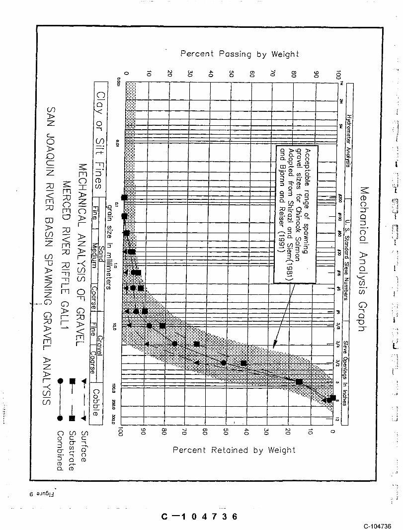
Conventionally, mechanical analysis results are plotted on semi-logarithmic graphs (Figure 9),and are referred to as gradation curves or mechanical analysis graphs. Gradation cm’vesgraphically present the percentage of particles retained and passing through specific sieveapertures. The gradation curve in Figure 9 represents clast composition at a sample location on

18

~1 04734C-104734

the Merced River. Appendix A contains gradation curves for all sampled riffles. The shadedarea on the graph represents the acceptable range of spawning gravel sizes for chinook salmon.This range is discussed in Part IV in the section titled Bulk Sampling Data Analysis on page 23.

Along the X-axis, sieve aperture sizes are arranged in logarithmic succession. Sieve numbersare arranged along the upper X axis. The sieve numbers refer to the nominal number ofopenings per inch: a #4 mesh sieve means that there are 4 openings per inch, a #200 mesh sievehas 200 openings per inch. The aperture dimensions (millimeters) corresponding to each sievesize may be read directly on the lower X-axis. Hence, a #4 mesh sieve corresponds to anaperture dimension of 5.5 millimeters.

The arithmetic Y-axis is divided into percentage values of retained weight plotted along the fightside of the graph and percent passing weight plotted on the left side of the graph. Theseinversely related percentages are dependent on the size distribution of the particles.

When the sieve analyses are plotted, the resultant curve will yield the percent passing (orinversely, percent retained) as a function of the aperture dimension and size range of the soil orgravel elasts. The shape and location of a gradation curve shows the general gradingcharacteristics of a soil or gravel. A very steep curve, with no tail, indicates a relatively uniformsoil or gravel with a small range of particle sizes. Conversely, a gentle curve indicates that awide range of.particle sizes exist. The gradation curves in Figure 9 represent a relatively well-mixed assortment of river clasts. Three curves are plotted on the graph in Figure 9: surfaceclasts, substrate elasts, and combined surface and substrate clasts. These curves are discussed inPart IV.

The median grain size, Ds0 is defined as the 50 percentile size, or the size which divides thedistribution such that 50% of the sample by weight is finer and 50% is coarser than this size.The median can be easily read from the 50% line in a particle-size gradation cur,,e. However, itindicates little about the range or skewness in particle sizes.

SURFACE SAMPLING

Surface samples were taken at 59 fifties using a modified Wolman method discussed below.Twenty samples were taken on the Tuolumne, twenty-two samples were taken on the Stanislaus,and seventeen samples were taken on the Merced.

The sampling method used to analyze and characterize stream-bed surface material at selectedfiffies was adapted from the grid method described by Wolman (1954). The Wolman method,

C--104735(3-104735

Percent P~ssing by Weigh~

_~ ~-~

......................

.

Percent Reteined by Weight

C--104736G-104736

with minor variation, was selected because of its relative simplicity and common usage. Theseattributes are beneficial in conducting field work under constrained conditions.

This method requires that individual stones be measured on the intermediate or b-axis by ruler orcalipers, or classified using square openings in a template. The distance between successivelysampled clasts is significant because of the propensity for clasts of similar size to imbricate. Toreduce serial correlation in the sample, the sample grid should be chosen so that successivelyselected clasts are at least several grain diameters apart (Church et al 1987). This wasaccomplished by the sampler taking a step between each sample point.

By statistical analysis on logarithmically transformed data, samples as small as forty clasts aresufficient to yield consistent estimates of mean size. Wolman used 60 clasts in onedemonstration of the met.hod, although he recommended a 100-clast sample as used in thisinvestigation.

To perform the Wolman method, one person paced along the head of the riffle. After eachpace, the person closed their eyes and reached into the water with a pointed finger. The fastparticle touched was picked up and the particle’s b-axis measured and recorded on the X,Volmandatasheet. The sampling person paced across the riffle head until water depth or velocity madesampling impossible or a shoreline was reached. Then the sampler took a pace upstream tobegin sampling in the other direction along a parallel grid line. This was continued until 100samples were recorded. The b-axis measurement was taken with a ruler scaled in phi units, withphi = -log~ of the b-axis diameter in millimeters.

PREFERRED SPAWNING GRAVEL AREA MEASUREMENT

Although not strictly a sampling method, this procedure for measuring the area of preferredspawning areas is included in the sampling methodology section. Preferred spawning gravelarea was measured at 53 Tuolurnne fifties, 65 Stanislaus fifties and 18 Merced fifties. Thepreferred spawning area is defined as the head of a riffle where flow ranges from one to threefeet per second and gravel is not compacted. Under these conditions, egg and alevin survivalrates are highest.

These measurements represent the most ideal, preferred spawning gravel. Salmon wil! likelyspawn in other areas not included in these measurements. The measured area extendsdownstream to segments of the riffle ~here vegetative encroachment, stream flow velocity, orobserved gravel dimension are insufficient to provide a preferred spawning area. The width ofthe preferred area was measured shoreline to shoreline. The length of the preferred area wasmeasured from the riffle head upstream. Measurements were taken with a 150 foot nylon tape.

C--’104737C-’104737

PART IV: SPAWNING GRAVEL RESOURCEASSESSMENT

BULK SAMPLING DATA ANALYSIS

To analyze the bulk sample data, the percent weight passing each sieve was plotted as agradation curve on a semi-log graph for each riffle. The surface, substrate, and combinedsurface and substrate gradations were plotted (Appendix A). Percentile diameters were readfrom the combined curve.

The gradation curves are presented in relation to an envelope of acceptable spawning gravel sizeranges. The envelope is represented as a shaded area on each particle accumulation curve. Theenvelope was generated using data from Shirazi and Seim (1981) and Bjornn and Reiser (1991).

The bulk sampling data were analyzed in three distinct elements: the surface sample, thesubstrate sample and a combination of both surface and substrate samples were plotted asgradation curves for each riffle (Appendix A). The surface and substrate samples were addedtogether on the combined spreadsheets in Appendix B. Appendix C contains spreadsheets forseparate surface and subsurface samples. The combined spreadsheets present aspects of centraltendency including geometric mean diameter (Dg), graphic geometric mean diameter (Dsg),standard deviation, skewness and kurtosis. Percent fines are also computed and presented withthe combined surface and substrate spreadsheets in Appendix B.

The mechanical analysis spreadsheets in Appendices B and C convert the size fraction weightsinto size fraction percent by weight. Because only a representative amount of particles passingthe #4 field sieve was retained for laboratory sieving, the spreadsheet calculates thepercentmoisture content of the laboratory sample, and proportionally distributes the adjusted weightamong the size fractions. The spreadsheets in Appendix B contains particle dimensions at theDgs, D~4, DT~, D~0, D~, D~, and D~. These dimensions are based onstandarddeviationincrements: the Da~ and D~ dimensions fall one standard deviation on either side of the median(D~0) and the Dgs and D~ dimensions fall two standard deviations on either side of the median.The DT~ and Dz~ dimensions were chosen to provide data intermediate within the first standarddeviation.

Table III is a tabulation of size values for substrate particles at the D~0 and D~0 passing sizefraction increments. The values are derived from the gradation curves in Appendix A.

The Ds0 and D~0 passing fractions were chosen to tabulate because: 1) the D~0 is a median valueand 2), the D~0 passing value defines the division between coarse sand and gravel in the shaded

C--104738C-104738

TABLEI[I

Comparison of D50 and D20 Sizes for Substrate Gravelby River

STANISLAUS TUOLUMNE MERCED~’~’~~’"~~~i~>5omo ~,~o mo ~,~o moiiii~ii’iiiii:i’: ~ ~!’.~i 12 1.8 10.5 0.8 14 10.5.! .i!!i..~i:!!iii2M[i" "° ’" " ’""40 11 12 10.5 13 7

10 2. 14 11 16 10.5

~ ~;~})~ 11 2 11 10 11.3 511 1.8 11 6 12.5 7

,?~,~<~ 11 0.8 11 3 12 10~}~ ~ 6 0.6 ~1 7 ~zs ~~ :: ~:~)~:~} 11 1.15 12 10

I 1 1.2 14 1211 8 10.5 211 8 !2 811 1.2 13.5 10.512 6 11.5 6.57 0.7 11.5 8

1!.5 2.2 15 1012 10 12.5 713 10 15 12.513 10.5 11.2 2.5

!2 10

~ea plotted on ~adafion cu~es in Append~ A. Addition~y, the D~0 v~ue ~te~ec~ ~e r~geof acceptable or suitable spawning gravel at 5 ~. A s~ple wi~ a Dzo p~sing vNue wNchdoes not exc~d 5 ~ fNls out of ~e suitable ~ge.

Table IV presents the m~ v~ues and v~s for ~ese size fractions. The non-p~e~enature of the data (non-norm~ dis~bufion and widely differing v~ces) preclude p~e~chypothesis tests to dete~ne whether si~ific~t differences ~ g~n size disMbufion e~stbetween each s~eam.

23

C--104739C-104739

However, a review of the means indicates that the D20 passing size fraction appears appreciablysmaller in the Stanislaus River. Otherwise, particle sizes at both size fractions appear equal inall streams. The smaller mean (4.91 ram) of the D2o passing fraction from the Stanislaus Kiverindicates that riffles on that stream may be more sand-laden than the other rivers.

TABLE IVMeans and Variances olD50 and D20 Fractions

42.202.22

Merced 12.24 2.13

Stanislaus 4.91 16.36l’uolurrme 7.54 12.69Merced 7.88 5.55

Table V tabulates fifties with a sand content which is greater than optimal for egg and alevinsurvival. This tabulation is derived from reading the gradation curves in Appendix A.

TABLE VSand-Laden Riffles

Stanislaus River Tuolumne RiverRiver Mile Riffle Number

36.00 36

42.20

45.20

49.20

50.90

04740C-104740

The plot of the gradation curves relative to the shaded area in Appendix A indicate the spawning "suitability of each analyzed riffle. Each analyzed riffle is represented by three curves: the surfacecurve, the substrate curve, and the combined curve. To represent suitable spawning gravel, thethree curves should fall within the shaded area. The plot of the combined curve is the mostimportant indicator of suitability because it represents the entire composition of the gravel used bythe salmon.

If the curves fall to the lett of the shaded area at the D~ passing fraction, that is if the size of thefraction is five millimeters or less, the gravel may be considered sand-laden and therefore less thansuitable for salmon spawning.

Sand-laden rittles on the Stanislaus and Tuolumne rivers are distributed downstream of a series ofgravel pits. The influence of these pits on the sand content of the downstream riffles compositionis not known. Nor is known the influence of bank erosion on gravel composition. The resolutionof these issues should be addressed.

To restore the sand-laden riffles, two approaches may be taken: 1) ripping the riffles to releasesand and 2) control of sand discharge into the stream above River Mile 50 on the StanislausRiver. Ripping is conventionally done with a bulldozer with ripper bars. Continuous maintenancewill likely be necessary to keep these riffles suitable for spawning gravel.

SURFACE SAM~PLING DATA ANALYSIS

Wolman counts were conducted simultaneously with bulk sampling for additional surface data.Appendix D presents plotted Wolman count curves. These curves indicate wide particle sizevariation. The curves also indicate that the surface size distribution of gravel in each riffle isroughly similar in each river. The shapes of the Wolman curves, with some exceptions, areroughly ~imilar, indicating that surface distribution of particles by size is roughly equal on allrivers.

ANALYSIS OF SPAWNING GRAVEL AREA

The spawning areas presented in this assessment are not the total spawning area available tochinook salmon in the three rivers. As discussed previously, chinook salmon will likely spawn inother areas not included in these measurements. The preferred spawning area extendsdownstream from the head of the riffle to points where vegetative encroachment, stream flowvelocity, or observed gravel dimension are insufficient to provide a preferred spawning area.Preferred spawning gravel is defined as gravel where flow velocity, water depth, and gravelcomposition are optimal for chinook salmon spawning. The area of each analyzed spawning riffleis presented in Tables VI, VII and VIII. Mean areas of the selected, preferred riffles ranged from

25

C--1 04741G-104741

4445 square feet on the Merced River to 3571 square feet on the Stanislaus River. The equalityof mean riffle areas may reflect hydrologic processes which preceded upstream dam construction.

River discharge, watershed area and morphology, underlying geology, and gradients are roughlythe same in each river.

26

C--104742C-104742

TABLE VIPreferred Spawning Gravel Area

Stanislaus River

Preferred Spawning Preferred SpawningGravel Gravel

River M ile Area River M lie Area(ft^2) (ft^2)

53.40 1800 45.00 1200

53.10 1296 44.60 7200

52.60 300 44.30 800

51.90 11990 44.00 2800

51.55 2500 43.70 1600~ ~ ~ ~ i 1 ~ ~ I l! ~i ~ ~ ~l t ~ ~ . tl~ ~ i ~ i i~ t~ ~ t tI~ ~ ~ ~ i~ ~ ~ " ~ ’~t~ ~ ~ ’~ ~

50.90 5250 43.00 3500

49.70 4785 42.20 6889!~I1 ~ ~t~ ~i1’ ~ ,~!~" ~!l l ll~!l ’ ,’:’ ~, l ~ ,i! I " f’ "’ It’ i’ll !~; i , ’ li~i ~"~l~ll ~"II I~ IiI~, I~’!~i "It’" t’ ’~ I - lllill~ ~ i I" ’

49.40 2070 40.40 540

49.20 8375 38.90 1800

48.80 4272 ~8.00 ~265

47.80 800 37.40 1800" i ’1’ I ’"~ ’t ! , , I

47.3 0 623 7 36.70 3 600

47.00 6000 36.00 3655¯ ¯ ’ l~ l ~ I " ~ ~l,~! ~ ~ ,. i : ~

46.70 800 35.60 1400.. , , I -.,, -. ,I.I 1,~i ~ .... ~, i ,

46.~0 1~00 35.00 3600

45.80 1200

45.20 5040 Mean Area(ft’2): 3571

27

~1 04743C-104743

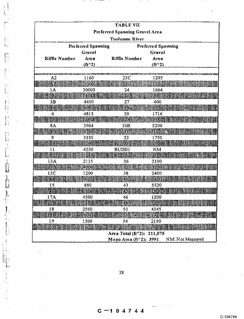
TAB LE VII

Preferred Spawning Gravel Area

Tuolunme River

Preferred Spavt~ing Preferred SpawningGravel Gravel

Riffle Number Area Riffle Number Area(ft^2) (ft^2)

A2 1160 23 C 1295

1A 30000 24 1664

3B 4400 27 400

6 4813 29 1716~ , ,,l!r i!i,~Ii lt~.,~, v !,-~,,

8A 3964 30B 5200

9 3350 32 1750

11 4250 R~D1

13A 2115 36 2100

13C 1200 38 2400

15 880 43 5520

17A 4500 46 1200

18 2560 50 4345

19 1500 54 2190

Area Total (ftA2): 211,575Mean Area (ft~2): 3991 NM: Not Meas~ed

C--1 04744C-104744

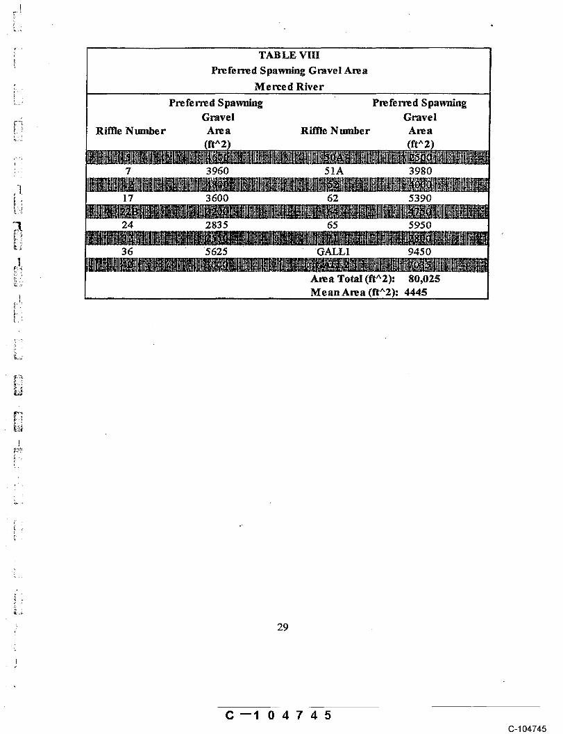
TAB LE VIIIr’ Preferred Spawning G~avei Area

~... Merced River~- .... Preferred Spawning Preferred Spawning

~:.~Gravel Gravel

~.. Riffle Number Area Riffle Number Area(ft^2) (ft^2)

).. 7 3960 51A , 3980

~ . 17 3600 62 5390

~ 24 2835 65 5950

36 "5625 G-ALL1 9450

29

C--1 04745C-104745

PART V: RIVER CONDITIONS

During the course of investigating the Stanislaus, Tuolumne, and Merced rivers, we observedsignificant conditions along each river which may affect salmon spawning habitat. Theseobservations are included in this part.

VEGETATION ENCROACHMENT

S~elected Tuolumne River riffle maps in Appendix E illustrate the vegetative encroachment onri£fles. Maps of fifties 2, 6, 8A, 9, 10, 11, 13A, 13B, 23D, and 28 portray invasion of vegetationinto the active stream channel. Vegetation along the river banks generally consists of trees,broad-leaf shrubs, and perennial aquatic grasses. This bank-side vegetation does not appear toaffect ri~es. However, vegetation in the active stream channel generally consists of mat-likegrasses whose root systems thoroughly invade the riffle gravel. These mat-like grasses appear totrap sand and silt and create islands in the channel. They appear to degrade the quality ofotherwise suitable spawning areas by preventing redd construction.

Vegetative encroachment may be the result of dam-impeded spring and early summer snow-meltrunoffwhich historically flushed these river systems. Increased nutrient loading from agriculturalrunoffmay promote vegetative growth.

COARSE GRAVEL DOVCNSTREAM OF DAMS

On the Merced and Tuolunme rivers, the suitability of salmon spawning habitat is degraded byexcessively coarse gravel and cobbles immediately downstream of the dams. Gradation curves inAppendix A for Tuolumne River Riffles A1, A2, and (marginally) 4A and for Merced Riffles 50,51, 52, 62, and 64, generally fall out on the coarse-side of the shaded area which defines suitablesalmon spawning gravel. Although coarse gravel is reasonably expected at the foothill/valleytransition where these riffles are located, the altered hydraulic regime resulting from theconstruction of dams has eliminated suffcient fines from the rivers immediately below the dams.The altered hydraulic regLrne resulting from dam construction enhances the erosive and scouringcapacity of the river at these points, thereby removing size fraction suitable for spawning.. Theanalyzed ri~es on the reaches immediately downstream of the dams were the only areas whichmay support spawning. Entire stretches within these reaches are scoured, particularly on portionsof the river underlain by bedrock. Where gravel exists, it is inappropriately large. Riffles A1, A7,and 3B illustrate the distribution of coarse gravels in the active channel.

~--1 04746C-104746

ENGINEERED ~ES ON THE TU’OLUMNE RIVER

Two sampled riffles, 1A and 2, on the Tuolumne River were constructed by Turlock and ModestoIrrigation Districts as mitigation for loss of spawning gravel caused by construction of upstreamdams. These riffles are constructed to provide artificial habitat for chinook salmon spawning on areach of river otherwise largely absent of preferred spawning gravel. Maps of these riffles arecontained in Appendix E. The alternation of coarse and less coarse gravel provides a series ofsimulated spawning habitats: the alternation mimics the transition from coarse gravel to lesscoarse gravel at natural riffle-heads. Note encroachment of’vegetation in Riffle 2 in Appendix E.

C--104747C-104747

REFERENCES CITED

Bell, Milo C. Fisheries Handbook of Engineering Requirements ~ld Biological Criteria,USCE Fish Passage Development and Evaluation Program, 1986.

Bjorrm, T. C. and D. W. Reiser. "Habitat Requirements of Salmonids in Streams," InInfluences Of Forest and Rangeland Management on Salmonid Fishes and TheirHabitats, American Fisheries Society Special Publication 19, W’dliam Meehan Editor.Bethesda, Maryland: American Fisheries Society, 1991.

California Department of Conservation, Erosion and Sediment Control Handbook, May 1978.

California Department offish and Game, Th~ Behavior and Reproduction of SalmonidFishes ina Small Coastal Stream, Fish Bulletin 94, 1953.

California Department offish and Game, Trout andSalmon Culture, Fish Bulletin 164, 1980.

California Department of Water Resources, Middle Sacramento River Spawning GravelStudy, 1984.

California Department of Water Resources, 1984. Upper Russian River Gravel andErosionStudy, 1984.

California Department of Water Resources, Sacramento River Spawning Gravel Studies-Executive Summary, 1985.

California Department of Water Resources, Upper Sacramento River Spawning GravelRestoration Project--Initial Pl~se, 1990.

Church, M. A., McLean, D.G and Wolcott F.J., "River Bed Gravels: Sampling andAnalysis." In Sediment Transport in Gravel-BedRivers, C. R. Thome et al, eds., John

Earth Analysts Science and Engineering, Don Pedro Project Fisheries Study Report (FERCArticle 3~, Project No. 2299), prepared for Turloek Irrigation District and ModestoIrrigation District, 1992.

Ett.ema, P,_, "Sampling Armor-Layer Sediments", Journal of Hydraulic Engineering, ASCE,1984.

Grost, R. T., Hubert, W.A., and Wesche, T.A~, "Field Comparison of Three Devices Used toSample Substrate in Small Streams", North American Journal of Fisheries Management,1991.

32

C--104748C-104748

Hinton, R. N., and Puckett, L.K., Some Measurements of the Relationship Between Streamflowand King Salmon Spawning Gravel on the Main Eel and Scn~th Fork Eel RiversCalifornia Department ofFish and Game Environmental Services Branch Admin. ReportNo. 74-1 1974.

Kondoif, G.M., "Gravel Issues", Conference Proceedings, Notes atnt Selected Abstracts fromthe Workshop on Central ~Iley Chinook Salmon, Da~,is, California, darmary 4-5, 1993.U.C. Davis, Department of Wildlife and Fisheries Biology, 1993.

Landis, P. 1993. Personal Communication.

Low, A. 1993. Personal Communication.

McNeil, W. ~I. and Ahnell, W.H., Success of Pink Salmon Spawning Relative to Size ofSpawning Bed Materials, Special Scientific Reprint, Fish No. 469. Washington, D.C.,U.S. Fish and Wildlife Service, 1964.

Mih, W.C., "A Review of Restoration of Stream Gravel for Spawning and Rearing of SalmonSpecies", Fisheries, Vol. 3, No.l, 1978.

Meehan, W.tL, Influences of Forest and Rangeland Management on Salmonid Fishes andTheir Habitats, American Fisheries Society Special Publication 19:83-138, 1991.

Shirazi, M. A., and Siem, W.K. et al, Characterization of Spawning Gravel and Stream SystemEvaluation, Salmon-Spawafing Gravel, A Renewable Resource in the Pacific Northwest,State of Washington, Water Resource Center Conference Proceedings, Pullman, WA,1981.

Spangler, NL G. and Handy, R.L., SoilEngineering, Fourth Edition. New York: Harper-Collins,

Smart,T.A., "Water Currents through Permeable Gravels and their Significance to SpawningSalmonids", Nature, Voi.173, No. 4399, 1953.

Thompson, K. "Determining Stream Flows for Fish Life" In: Proceedings, Instream FlowRequirement Workshop, Pacific Northwest River Basin Committee, 1972.

Vaux, W.B., Interchange of Stream an~l Intergravel Water in a Salmon Spa~,ning R/if/e, SpecialScientific Report, Fish No. 405, United States Fish and Wildlife Service, 1962.

Wolman, M. G., 1954. "A Method of Sampling Coarse River-Bed Material." TransactionsAmerican Geophysical Union, Vol. 35, No. 6, 1954.

~--~ 04749C-104749

Young, M. K. et al, "Selection of Measures of Substrate Composition to Estimate Sur,,ival toEmergence of Salrnonids and to Detect Changes in Stream Substrates", North AmericanJournal of Fisheries Management, ~rol. 11, 1991.

34

~ .

C--104750(3-104750

CONVERSION FACTORS

TO Convect toQuantity To Conve¢l from Metric Umt To Customary Unit Mu|t=ply

Un== ByCustomary Unit :

Length m,llimetres (ram) inches (in) 0.03937 25.4centimetres (cm) for snow depth inches (in} 0.3937 2.54metres (m) feet (ft) 3.2808 0.3048kilometres (kin} miles (mi) 0.62139 1.6G93

Area square millimetres (mm=) square inches (ina) O.CO 155 645.16square metres (m~) square feet fit=} 10.764 0.09290hectares (ha) acres (ac} 2.4710 0.40469square kilomettes (km~) square miles (mi=) 0.3861 2.590

Volume lilies (1’) "gallon~ (gal) "0.26417’ 3.7854 .megalitres million gallons ( 1CP gai) 0.26417 3.7854cubic metres (ms) cubic feet (ft=} 35.315 0.02831cubic metres (m=) cubic yards (yd=) 1.308 0.76455cubic dekametres (dam=) acre-feet (ac-ft} 0.8107 1.2335

Flow cubic metres per second (mS/s} cubic feet per second 35.315 0.028317(ft=!s)

litres per minute (L/min) gallons per minute 0.26417 3.7854(gal/min)

litres per day (L/day) gallons per day (gal/day) 0.26417 3.7854megalitre.s per day (MLiday) million gallons 0.2~. 17 3.7854

per day (mgd}cubic dek.*.metres per day acre-feet per day (ac- 0.8107 1.2335

(damS/day) ft/day)

Mass kilograms (kg) pounds (Ib) 2.2046 0.4535_9megagrams (Mg}. tons (short. 2.003 lb) 1.1023 0.90718

Velocity , metres per second (m/s) feet per second (ft/s) 3.2808 0.3048

Power kilowatts (kW) horsepower (hp) 1.3405 0.746

Pressure kilopascals (kPa} pounds per square inch (~; 14505 6.8948

kiiopascals (kPa) feet head of water 0.33456 2.969

Specific Capacity litres per minute per metre gallons per minute per 0.(38~52 12.419drawdown foot drawdown

Concentration milligrams per litre (mg/L) parts per million (ppm} 1.0

Electrical Con- microsiemens per centtmetre micromhos per centimetre 1.0 1ductivity {uS/cm}

Temperature degrees Celsius (~C) degrees Fahrenheit (°F) (1.8 X ~C}-}-32 (=F--32)/I.

C--1 04751C-104751