1

SAN FRANCISCO STATE UNIVERSITY

From the Geographical Cycle to Chaos Theory:

A Century of Geomorphic Concepts

Submitted to

Dr. Jerry Davis

Geography 810: Seminar in Geomorphology

By

Kevin Jackson

16 May 2001

2

Abstract A review of the evolution of geomorphic concepts and theories during the past century reveals that all may contribute to the understanding of landform development, but that it is a matter of scale in regards to time and space as to which best explains particular questions. W. M. Davis’ (1899) geographical cycle, in its simplicity, may best explain landform development at a grand scale of continents and millennia. The smaller scale implicit in the systems approach advocated by Strahler (1952) and the concern with equilibria that followed (Hack 1960, 1975; Chorley 1962; Chorley and Kennedy 1971) helped answer questions about the relationship between process and form. But at the smaller scale infrequent/high-magnitude events became catastrophes and concepts such as disequilibrium, nonequilibrium, nonlinear dynamical theory, and chaos theory have been employed to explain landform development (Renwick 1992; Phillips 1992a, 1992b; Malanson 1992). Recognizing the value in both grand and small-scale approaches are geomorphologists who try to reconcile the two (Schumm and Lichty 1965, Kennedy 1992, Mayer 1992). As the accumulation of data increases, and computer systems are developed and refined, chaos theory holds promise for explaining landform development and making long-term predictions (Malanson et al. 1990, Phillips 1992b).

3

Introduction Theory attempts to explain how and why things happen. When beginning to study landforms the student of geomorphology is likely to feel overwhelmed by the complexity of the subject matter and may turn to current or past theories in order to understand how it all works and fits together. Unfortunately, the various theories at hand may appear as complex and diverse as the landforms they attempt to explain. Additionally, the discipline’s scholars have a tendency to malign one theory in favor of another in their search for the truth. What is the student to believe?, to follow?, to use? For centuries geomorphologists have worked hard at getting at the truth. But as it stands, no single theory has all the answers for geomorphologists. No single theory distills the complexity of earth’s landforms into one simple truth. This paper attempts to examine the evolution of geomorphic thought during the past century. The simplicity of W. M. Davis’ (1899) geographical cycle proved popular but left many a scientist wanting. A. N. Strahler (1952) hoped to fill the scientific void by calling on his colleagues to employ quantitative analysis to geomorphology. Answering Strahler’s call were J. T. Hack who touted dynamic equilibrium theory, and R. J. Chorley (1962, and Kennedy 1971) who employed general systems theory. Expanding on the works of these earlier scientists, geomorphologists of the last quarter century developed concepts concerning equilibrium, disequilibrium, and nonequilibrium (Renwick 1992); nonlinear dynamical theory (Phillips 1992b); and chaos theory (Malanson et al. 1990). Each theory is examined so that its essential idea is presented graphically as well as verbally. This is done chronologically in order to present the evolution of one theory to the next and the progression of geomorphic concepts. This should allow the student to ascertain the value of each theory or approach and which one(s), if any, to use when studying landforms. The Geographical Cycle Charles G. Higgins (1975) suggests that the modern era of geomorphology began in the year 1877 with the publication of G. K. Gilbert's Report on the geology of the Henry Mountains. Despite the few broad generalizations about landform development he allowed himself, such as the "law of uniform slope," the "law of structure," the "law of divides," and the "tendency to equality of action, or to the establishment of a dynamic equilibrium" (Gilbert 1877: 115-116, 123), Gilbert considered himself an "investigator" rather than a "theorist," who he described as someone who fails to test his hypothesis adequately. Thus Gilbert, interested mainly in the relationships between process and form, bequeathed future geomorphologists a wealth of insightful works but left the formulation of broad theories of landscape development to others (Higgins 1975). William Morris Davis (1899), in his paper The Geographical Cycle, posited "the first truly general theory . . . of landscape development" (Higgins 1975: 6). Feeling that “geography has already suffered too long from the disuse of imagination, invention, deduction, and the various other mental faculties that contribute towards the attainment of a well-tested explanation,” he presented a theory in which “all the varied forms of the

4

lands are dependent upon – or, as the mathematician would say, are functions of – three variable quantities, which may be called structure, process, and time” (Davis 1899: 483-4, 481).

In the beginning, when the forces of deformation and uplift determine the structure and attitude of a region, the form of its surface is in sympathy with its internal arrangement, and its height depends on the amount of uplift that it has suffered. If its rocks were unchangeable under the attack of external processes, its surface would remain unaltered until the forces of deformation and uplift acted again; and in this case structure would be alone in control of form. But no rocks are unchangeable; even the most resistant yield under the attack of the atmosphere, and their waste creeps and washes downhill as long as any hills remain; hence all forms, however high and however resistant, must be laid low, and thus destructive process gains rank equal to that of structure in determining the shape of a landmass. Process cannot, however, complete its work instantly, and the amount of change from initial form is therefore a function of time. Time thus completes the trio of geographical controls, and is, of the three, the one of most frequent application and of most practical value in geographical description (Davis 1899: 481-482).

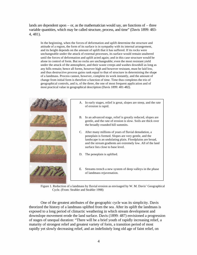
Figure 1. Reduction of a landmass by fluvial erosion as envisaged by W. M. Davis’ Geographical

Cycle. (From: Strahler and Strahler 1998) One of the greatest attributes of the geographic cycle was its simplicity. Davis theorized the history of a landmass uplifted from the sea. After its uplift the landmass is exposed to a long period of climactic weathering in which stream development and downslope movement erode the land surface. Davis (1899: 487) envisioned a progression of stages of unequal duration: “There will be a brief youth of rapidly increasing relief, a maturity of strongest relief and greatest variety of form, a transition period of most rapidly yet slowly decreasing relief, and an indefinitely long old age of faint relief, on

A. In early stages, relief is great, slopes are steep, and the rate of erosion is rapid.

B. In an advanced stage, relief is greatly reduced, slopes are gentle, and the rate of erosion is slow. Soils are thick over the broadly rounded hill summits.

C. After many millions of years of fluvial denudation, a

peneplain is formed. Slopes are very gentle, and the landscape is an undulating plain. Floodplains are broad, and the stream gradients are extremely low. All of the land surface lies close to base level.

D. The peneplain is uplifted.

E. Streams trench a new system of deep valleys in the phase of landmass rejuvenation.

5

which further changes are exceedingly slow.” The final product of this long period of erosion is “an almost featureless plain (a peneplain) showing little sympathy with structure, and controlled only by a close approach to baselevel” (Davis 1899: 497). Another period of uplift would begin this cycle anew. Davis’ geographical cycle proved immensely popular. Higgins (1975) writes that Davis and his followers would go on to apply this cyclic concept, which was originally intended to explain landform development in humid temperate climates, to arid, glacial, karst, and littoral landscapes. The theory would produce other cycles of landform development including the “Normal Cycle,” the “Fluvial Cycle,” the “Erosion Cycle,” the “Geomorphic Cycle,” and the “Humid Cycle.” And the trio of controls: structure, process, and time; would be changed by Davis’ followers to structure, process and stage. But the true value of this theory lay not in any details or modifications but in its simple explanation of genetic landform development through an understanding of gravitational force, climate, and tectonic uplift. The Quantitative Revolution Due to its simple “logic, detailed terminology and its apparent applicability to a variety of systems and landforms” (Anhert 1996: 325), Davis’ geographical cycle remained popular for half a century until 1952 when A. N. Strahler published his Dynamic Basis of Geomorphology. As part of the quantitative revolution, Strahler (1952: 924) found Davis’ historical approach to be an overly “explanatory-descriptive method of study” and believed that “If geomorphology is to achieve full stature as a branch of geology operating upon the frontier of research into fundamental principles and laws of earth science, it must turn to the physical and engineering sciences and mathematics for vitality which it now lacks.” Although Strahler (1952) stated that dynamic geomorphologists could not ignore historical evidence in existing landscapes, he felt that the function of time was an essential element separating historical geomorphology and dynamic geomorphology. “The student of processes and forms per se is continually asking ‘What happens?’; the historical student keeps raising the question ‘What happened?’” (Strahler 1952: 924). Strahler (1952) was not putting forth a new theory perhaps but he did call for a completely new approach to geomorphological studies, grounding the discipline to the basic principles of mechanics and fluid dynamics (See Table 1). He suggested that geomorphic processes, such as weathering, erosion, transportation and deposition, be treated as manifestations of gravitational and molecular shear stresses. These stresses and processes could be measured mathematically to produce models quantifying statements of geomorphic process and form.

6

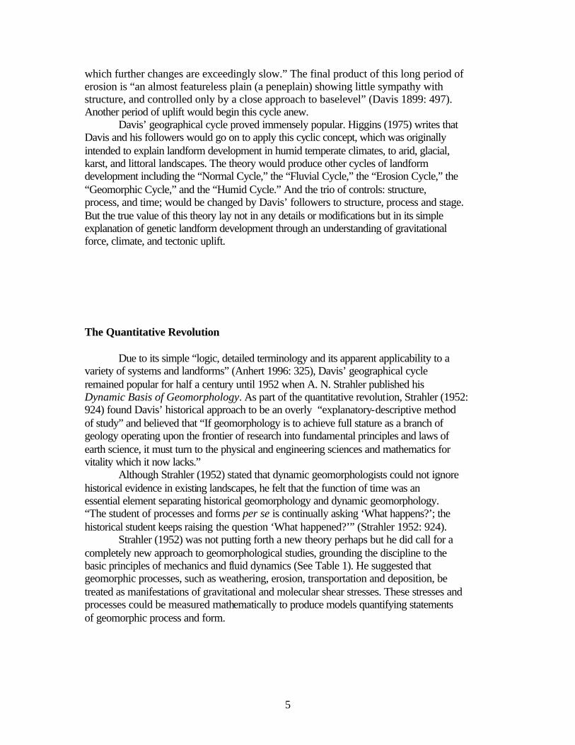
Table 1. Dynamic Basis of Geomorphology showing processes as manifestations of gravitational

and molecular shear stresses (From Strahler 1952).

Borrowing thermodynamic principles from physics and chemistry, Strahler (1952) suggested geomorphic forms and processes be studied in terms of dynamic systems in which the transformations of mass and energy are considered as functions of time. Geomorphic processes, operating in clearly defined systems, such as drainage systems, could be isolated for analysis. Strahler (1952: 935) recognized two types of systems: “(1) the closed system which has a clearly defined boundary through which neither materials nor energy are exchanged, and (2) the open system which exchanges either material or energy (or both) with outside environments.” He equated open systems with streams and glaciers, asserting that they are self-regulating mechanisms, achieving a time-independent steady state by balancing an inflow of mass and energy with their outflow. No one states this call for quantitative studies more succinctly than Strahler (1952: 937) himself:

In summary, the proposed program for future development of geomorphology on a dynamic-quantitative basis requires the following steps: (1) study of geomorphic processes and landforms as various kinds of responses to gravitational and molecular shear stresses acting upon materials behaving characteristically as elastic or plastic solids, or viscous fluids; (2) quantitative determinations of landform characteristics and causative factors; (3) formulation of empirical equations by methods of mathematical statistics; (4) building of the concept of open dynamic systems and steady states for all phases of geomorphic processes; and finally (5) the deduction of general mathematical models to serve as quantitative natural laws.

7

Dynamic Equilibrium and General Systems Theory Writing eight years after the publication of Strahler’s (1952) paper and building upon its content, John T. Hack (1960) took the geographical cycle to task again, this time in favor of the concept of dynamic equilibrium, a term he borrowed from G. K. Gilbert (1877). Hack pointed to studies showing evidence of almost continuous diastrophism through time in order to discredit cyclic geomorphic theories, such as Davis’, that were based upon periodic uplift of the earth’s crust. The tens of millions of years it takes to reduce a mountain to low relief allows time for repeated major tectonic and climatic changes, such as those that have occurred in the Tertiary and Quaternary. Because of this there is scant evidence that a Davisian cycle has ever been completed (Anhert 1996). Hack (1960: 81) wrote that the concept of dynamic equilibrium could better explain landform development:

The landscape and the processes molding it are considered a part of an open system in a steady state of balance in which every slope and every form is adjusted to every other. Changes in topographic form take place as equilibrium conditions change, but it is not necessary to assume that the kind of evolutionary changes envisaged by Davis ever occur.

Hack was essentially stating that long-term landform development results from spatial linkages of short-term processes (Mayer 1992). Hack (1975) was later careful to point out that, unlike the geographic cycle of Davis, dynamic equilibrium is not an evolutionary model. Dynamic equilibrium is a principle to be used to study and explain specific landscape features with the assumption that the landscape has developed over a long period of continual erosion. He admitted that landscape changes might evolve during a cycle as Davis described them, but that the principle of dynamic equilibrium was better suited to explain topographic forms and the processes acting on them (Hack 1975). Richard J. Chorley (1962) also elaborated on the concepts mentioned in Strahler’s (1952) paper in Geomorphology and General Systems Theory. He advocated an open-systems approach to studying landforms rather than a closed-system historical approach. Describing Davis’ geomorphic cycle as a closed system, Chorley stated that uplift provided initial energy that decreased as degradation proceeded to a state of minimum free energy and topographic differences. Closed systems experience an increase in entropy, implying an irreversibility of events as described in the geographical cycle (Chorley 1962). In contrast, an open system, exemplified by a reach of stream, continually adjusts input and output in a tendency towards a steady state. “Open systems thus may maintain their organization and regularity of form, in a continual exchange of their component materials” (Chorley 1962: B6). These components and their relationship can be recognized statistically. Distancing systems theory even further from the geographical cycle, Chorley maintained that the dynamic equilibrium of a steady state, towards which an open system gravitates, is maintained for a very short duration, perhaps days or even minutes. This continuum of adjustments and brief equilibriums tends to make considerations of previous history hypothetical and irrelevant (Chorley 1962). Chorley, with B. A. Kennedy (1971), later expanded upon this idea of a systems approach in physical geography. Since the real world is immense and continuous, a

8

scientist, in order to make a meaningful study, must examine only a small section. The student must not only look at the components of the individual section but also at its links to other sections. These sections can be called systems. “The real world, then, can be viewed as comprising sets of interlinked systems at various scales and of varying complexity, which are nested into each other to form a systems hierarchy” (Chorley and Kennedy 1971: 1).

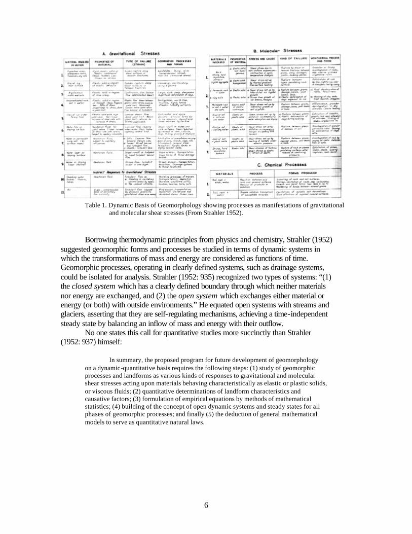
This seems fairly simple to comprehend. However, as the concepts of systems and equilibrium evolved they became as complex as the real world. Chorley and Kennedy (1971) recognized eleven different types of systems but found four relevant to physical geography (See figure 2).

(1) Morphological systems are comprised of physical, or morphological, properties and the relationships between them.

(2) Cascading systems are composed of a chain of subsystems linked by a flow, or cascade, of mass or energy.

(3) Process-response systems link at least one morphological system with at least one cascading system in order to demonstrate how form is related to process.

(4) Control systems are process response systems in which the key components are controlled by some intelligence (man).

Figure 2. Schematic illustrations of the four types of systems identified by Chorley and Kennedy

(1971). Feedback mechanisms are an essential component of the systems concept.

Chorley and Kennedy (1971) write that positive feedback reinforces the effects of an externally induced change and causes a relatively short burst of snowballing self-destructive activity. Negative feedback tends to restrain the effect of an externally induced change and to help a system regulate and repair itself. This leads to open system or dynamic equilibrium.

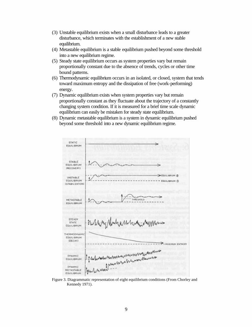
Since systems only tend towards equilibrium, and may only achieve equilibrium for very short periods, it “is a highly ambiguous state which presents many different aspects and is the subject of a wide variety of definitions” (Chorley and Kennedy 1971: 201). Chorley and Kennedy (1971) outline eight varieties of equilibrium (See Figure 3).

(1) Static equilibrium exists when there is no change in certain system properties. (2) Stable equilibrium occurs when a system tends to return to a previous

equilibrium condition after being disturbed by limited external forces.

9

(3) Unstable equilibrium exists when a small disturbance leads to a greater disturbance, which terminates with the establishment of a new stable equilibrium.

(4) Metastable equilibrium is a stable equilibrium pushed beyond some threshold into a new equilibrium regime.

(5) Steady state equilibrium occurs as system properties vary but remain proportionally constant due to the absence of trends, cycles or other time bound patterns.

(6) Thermodynamic equilibrium occurs in an isolated, or closed, system that tends toward maximum entropy and the dissipation of free (work-performing) energy.

(7) Dynamic equilibrium exists when system properties vary but remain proportionally constant as they fluctuate about the trajectory of a constantly changing system condition. If it is measured for a brief time scale dynamic equilibrium can easily be mistaken for steady state equilibrium.

(8) Dynamic metastable equilibrium is a system in dynamic equilibrium pushed beyond some threshold into a new dynamic equilibrium regime.

Figure 3. Diagrammatic representation of eight equilibrium conditions (From Chorley and

Kennedy 1971).

10

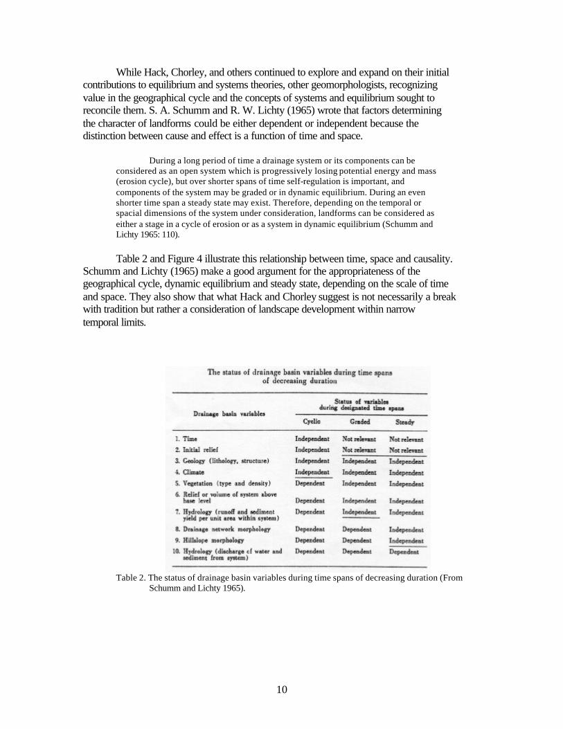
While Hack, Chorley, and others continued to explore and expand on their initial contributions to equilibrium and systems theories, other geomorphologists, recognizing value in the geographical cycle and the concepts of systems and equilibrium sought to reconcile them. S. A. Schumm and R. W. Lichty (1965) wrote that factors determining the character of landforms could be either dependent or independent because the distinction between cause and effect is a function of time and space.

During a long period of time a drainage system or its components can be

considered as an open system which is progressively losing potential energy and mass (erosion cycle), but over shorter spans of time self-regulation is important, and components of the system may be graded or in dynamic equilibrium. During an even shorter time span a steady state may exist. Therefore, depending on the temporal or spacial dimensions of the system under consideration, landforms can be considered as either a stage in a cycle of erosion or as a system in dynamic equilibrium (Schumm and Lichty 1965: 110). Table 2 and Figure 4 illustrate this relationship between time, space and causality.

Schumm and Lichty (1965) make a good argument for the appropriateness of the geographical cycle, dynamic equilibrium and steady state, depending on the scale of time and space. They also show that what Hack and Chorley suggest is not necessarily a break with tradition but rather a consideration of landscape development within narrow temporal limits.

Table 2. The status of drainage basin variables during time spans of decreasing duration (From

Schumm and Lichty 1965).

11

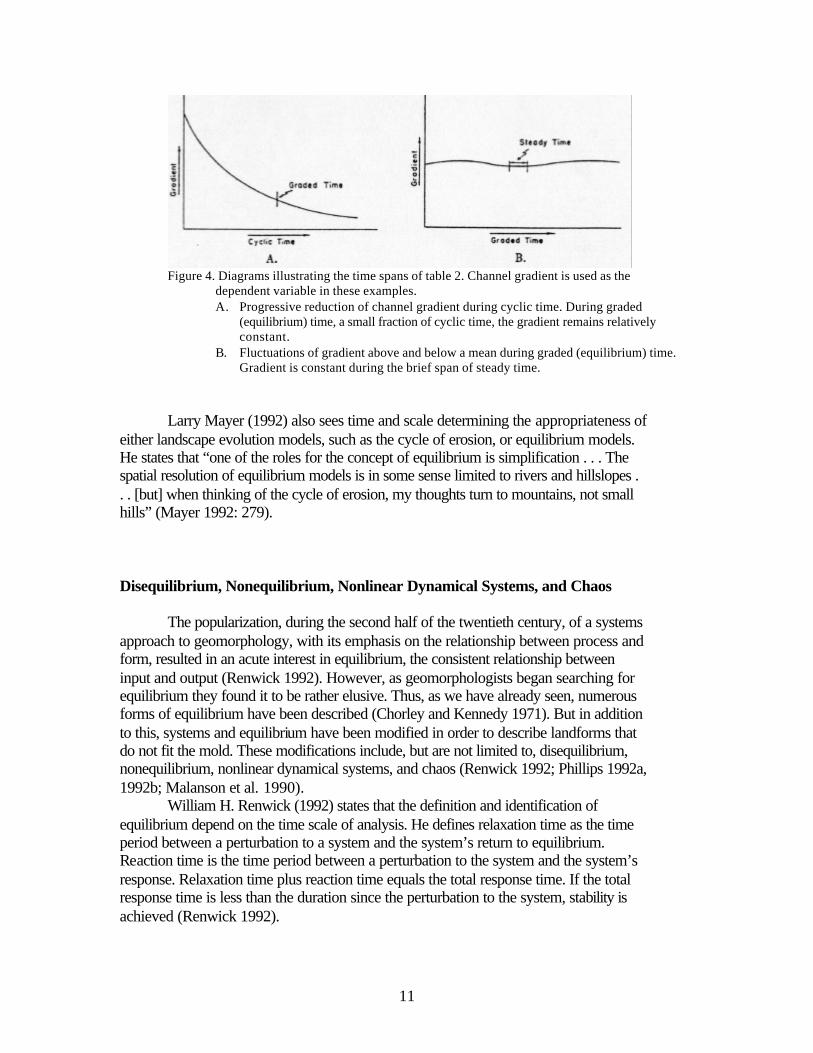
Figure 4. Diagrams illustrating the time spans of table 2. Channel gradient is used as the

dependent variable in these examples. A. Progressive reduction of channel gradient during cyclic time. During graded

(equilibrium) time, a small fraction of cyclic time, the gradient remains relatively constant.

B. Fluctuations of gradient above and below a mean during graded (equilibrium) time. Gradient is constant during the brief span of steady time.

Larry Mayer (1992) also sees time and scale determining the appropriateness of

either landscape evolution models, such as the cycle of erosion, or equilibrium models. He states that “one of the roles for the concept of equilibrium is simplification . . . The spatial resolution of equilibrium models is in some sense limited to rivers and hillslopes . . . [but] when thinking of the cycle of erosion, my thoughts turn to mountains, not small hills” (Mayer 1992: 279).

Disequilibrium, Nonequilibrium, Nonlinear Dynamical Systems, and Chaos

The popularization, during the second half of the twentieth century, of a systems

approach to geomorphology, with its emphasis on the relationship between process and form, resulted in an acute interest in equilibrium, the consistent relationship between input and output (Renwick 1992). However, as geomorphologists began searching for equilibrium they found it to be rather elusive. Thus, as we have already seen, numerous forms of equilibrium have been described (Chorley and Kennedy 1971). But in addition to this, systems and equilibrium have been modified in order to describe landforms that do not fit the mold. These modifications include, but are not limited to, disequilibrium, nonequilibrium, nonlinear dynamical systems, and chaos (Renwick 1992; Phillips 1992a, 1992b; Malanson et al. 1990).

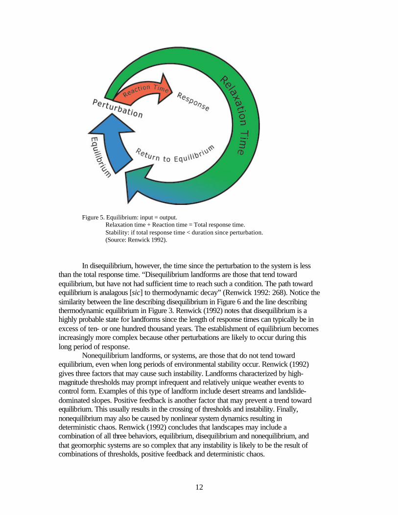
William H. Renwick (1992) states that the definition and identification of equilibrium depend on the time scale of analysis. He defines relaxation time as the time period between a perturbation to a system and the system’s return to equilibrium. Reaction time is the time period between a perturbation to the system and the system’s response. Relaxation time plus reaction time equals the total response time. If the total response time is less than the duration since the perturbation to the system, stability is achieved (Renwick 1992).

12

Figure 5. Equilibrium: input = output. Relaxation time + Reaction time = Total response time. Stability: if total response time < duration since perturbation. (Source: Renwick 1992). In disequilibrium, however, the time since the perturbation to the system is less

than the total response time. “Disequilibrium landforms are those that tend toward equilibrium, but have not had sufficient time to reach such a condition. The path toward equilibrium is analagous [sic] to thermodynamic decay” (Renwick 1992: 268). Notice the similarity between the line describing disequilibrium in Figure 6 and the line describing thermodynamic equilibrium in Figure 3. Renwick (1992) notes that disequilibrium is a highly probable state for landforms since the length of response times can typically be in excess of ten- or one hundred thousand years. The establishment of equilibrium becomes increasingly more complex because other perturbations are likely to occur during this long period of response.

Nonequilibrium landforms, or systems, are those that do not tend toward equilibrium, even when long periods of environmental stability occur. Renwick (1992) gives three factors that may cause such instability. Landforms characterized by high-magnitude thresholds may prompt infrequent and relatively unique weather events to control form. Examples of this type of landform include desert streams and landslide-dominated slopes. Positive feedback is another factor that may prevent a trend toward equilibrium. This usually results in the crossing of thresholds and instability. Finally, nonequilibrium may also be caused by nonlinear system dynamics resulting in deterministic chaos. Renwick (1992) concludes that landscapes may include a combination of all three behaviors, equilibrium, disequilibrium and nonequilibrium, and that geomorphic systems are so complex that any instability is likely to be the result of combinations of thresholds, positive feedback and deterministic chaos.

13

Figure 6. Examples of equilibrium, disequilibrium, and nonequilibrium landform behavior (From

Renwick 1992).

Figure 7. An illustration of stream system in disequilibrium converging to equilibrium (From

Renwick 1992).

14

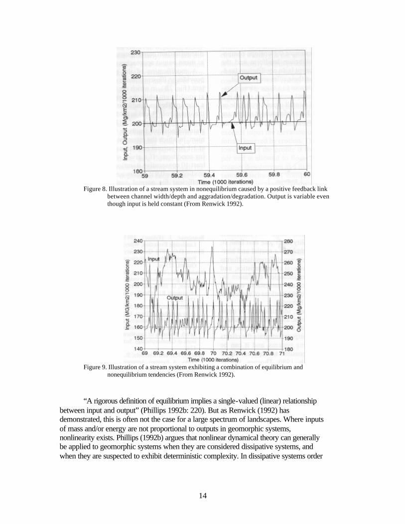
Figure 8. Illustration of a stream system in nonequilibrium caused by a positive feedback link

between channel width/depth and aggradation/degradation. Output is variable even though input is held constant (From Renwick 1992).

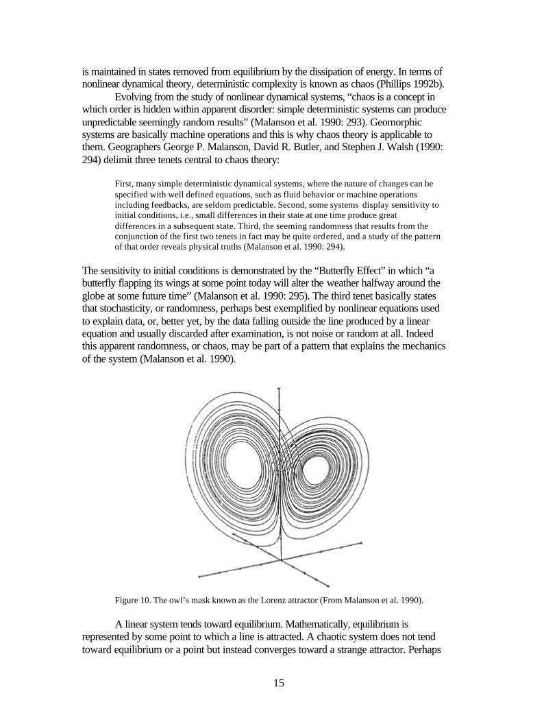
Figure 9. Illustration of a stream system exhibiting a combination of equilibrium and

nonequilibrium tendencies (From Renwick 1992). “A rigorous definition of equilibrium implies a single-valued (linear) relationship

between input and output” (Phillips 1992b: 220). But as Renwick (1992) has demonstrated, this is often not the case for a large spectrum of landscapes. Where inputs of mass and/or energy are not proportional to outputs in geomorphic systems, nonlinearity exists. Phillips (1992b) argues that nonlinear dynamical theory can generally be applied to geomorphic systems when they are considered dissipative systems, and when they are suspected to exhibit deterministic complexity. In dissipative systems order

15

is maintained in states removed from equilibrium by the dissipation of energy. In terms of nonlinear dynamical theory, deterministic complexity is known as chaos (Phillips 1992b).

Evolving from the study of nonlinear dynamical systems, “chaos is a concept in which order is hidden within apparent disorder: simple deterministic systems can produce unpredictable seemingly random results” (Malanson et al. 1990: 293). Geomorphic systems are basically machine operations and this is why chaos theory is applicable to them. Geographers George P. Malanson, David R. Butler, and Stephen J. Walsh (1990: 294) delimit three tenets central to chaos theory:

First, many simple deterministic dynamical systems, where the nature of changes can be specified with well defined equations, such as fluid behavior or machine operations including feedbacks, are seldom predictable. Second, some systems display sensitivity to initial conditions, i.e., small differences in their state at one time produce great differences in a subsequent state. Third, the seeming randomness that results from the conjunction of the first two tenets in fact may be quite ordered, and a study of the pattern of that order reveals physical truths (Malanson et al. 1990: 294).

The sensitivity to initial conditions is demonstrated by the “Butterfly Effect” in which “a butterfly flapping its wings at some point today will alter the weather halfway around the globe at some future time” (Malanson et al. 1990: 295). The third tenet basically states that stochasticity, or randomness, perhaps best exemplified by nonlinear equations used to explain data, or, better yet, by the data falling outside the line produced by a linear equation and usually discarded after examination, is not noise or random at all. Indeed this apparent randomness, or chaos, may be part of a pattern that explains the mechanics of the system (Malanson et al. 1990).

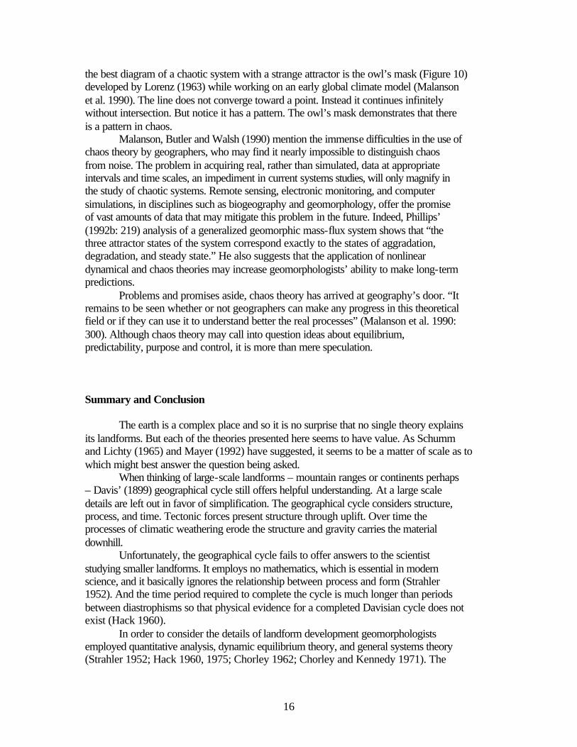
Figure 10. The owl’s mask known as the Lorenz attractor (From Malanson et al. 1990).

A linear system tends toward equilibrium. Mathematically, equilibrium is represented by some point to which a line is attracted. A chaotic system does not tend toward equilibrium or a point but instead converges toward a strange attractor. Perhaps

16

the best diagram of a chaotic system with a strange attractor is the owl’s mask (Figure 10) developed by Lorenz (1963) while working on an early global climate model (Malanson et al. 1990). The line does not converge toward a point. Instead it continues infinitely without intersection. But notice it has a pattern. The owl’s mask demonstrates that there is a pattern in chaos. Malanson, Butler and Walsh (1990) mention the immense difficulties in the use of chaos theory by geographers, who may find it nearly impossible to distinguish chaos from noise. The problem in acquiring real, rather than simulated, data at appropriate intervals and time scales, an impediment in current systems studies, will only magnify in the study of chaotic systems. Remote sensing, electronic monitoring, and computer simulations, in disciplines such as biogeography and geomorphology, offer the promise of vast amounts of data that may mitigate this problem in the future. Indeed, Phillips’ (1992b: 219) analysis of a generalized geomorphic mass-flux system shows that “the three attractor states of the system correspond exactly to the states of aggradation, degradation, and steady state.” He also suggests that the application of nonlinear dynamical and chaos theories may increase geomorphologists’ ability to make long-term predictions. Problems and promises aside, chaos theory has arrived at geography’s door. “It remains to be seen whether or not geographers can make any progress in this theoretical field or if they can use it to understand better the real processes” (Malanson et al. 1990: 300). Although chaos theory may call into question ideas about equilibrium, predictability, purpose and control, it is more than mere speculation.

Summary and Conclusion The earth is a complex place and so it is no surprise that no single theory explains its landforms. But each of the theories presented here seems to have value. As Schumm and Lichty (1965) and Mayer (1992) have suggested, it seems to be a matter of scale as to which might best answer the question being asked. When thinking of large-scale landforms – mountain ranges or continents perhaps – Davis’ (1899) geographical cycle still offers helpful understanding. At a large scale details are left out in favor of simplification. The geographical cycle considers structure, process, and time. Tectonic forces present structure through uplift. Over time the processes of climatic weathering erode the structure and gravity carries the material downhill. Unfortunately, the geographical cycle fails to offer answers to the scientist studying smaller landforms. It employs no mathematics, which is essential in modern science, and it basically ignores the relationship between process and form (Strahler 1952). And the time period required to complete the cycle is much longer than periods between diastrophisms so that physical evidence for a completed Davisian cycle does not exist (Hack 1960). In order to consider the details of landform development geomorphologists employed quantitative analysis, dynamic equilibrium theory, and general systems theory (Strahler 1952; Hack 1960, 1975; Chorley 1962; Chorley and Kennedy 1971). The

17

landscape was compartmentalized into systems where process and form were considered as transformations of mass and energy. It was originally thought that the relationship between the input and output of mass and/or energy of a system would tend toward and equilibrium or steady state (Hack 1960, 1975; Chorley 1962; Chorley and Kennedy 1971). But geomorphologists soon realized that a large portion of landforms did not tend toward equilibrium or steady states, or, if they did the duration of equilibrium or a steady state was rather brief and fleeting with the period of adjustment between a perturbation and equilibrium lasting up to 100,000 years (Schumm and Lichty 1965, Renwick 1992). Consequently, some geomorphologists have attempted to modify concepts of equilibrium to include not only equilibrium but also disequilibrium and nonequilibrium (Renwick 1992). Disequilibrium is a term that describes a system in this long adjustment period as it tends toward equilibrium but is not yet there (Renwick 1992). Landforms that do not tend toward equilibrium, even when long periods of environmental stability occur, are said to exhibit nonequilibrium behavior. This tendency toward nonequilibrium might be the result of high-magnitude thresholds, positive feedback, or nonlinear system dynamics, or all three (Renwick 1992). When geomorphologists statistically analyzed the relationship between process and form they would plot the data to see if it followed a line tending toward equilibrium. Often there was data falling well outside the line that was thought to be random and would be explained away as noise. Recently, nonlinear dynamical theory and chaos theory have been employed to explain this outlying data, not as noise, but as deterministic chaos (Phillips 1992b, Malanson et al. 1990). A chaotic system tends not toward equilibrium, but toward a strange attractor (Malanson et al. 1990), which may correspond to aggradation, degradation or steady state (Phillips 1992b). As data is increasingly accumulated and computer systems are developed and refined, chaos theory may help to increase our understanding of landform development and to make long-term predictions (Phillips 1992b). But it does seem to come down to the scale of time and space. The perturbations, or catastrophic events, that seem to prohibit the understanding of landforms at a systems level, or at least make it utterly complex, are merely straightforward high-magnitude/low-frequency events at the geographical cycle level. Barbara A. Kennedy, who wrote Physical Geography: A Systems Approach with R. J. Chorley (1971), recently addressed this issue of scale:

It seems to me that we have a choice to make in our view of things: if we take as our central focus equilibria, then we will also see catastrophes abounding; alternatively, if we simply envisage a sequence of events of all, physically-possible shapes and sizes, then both equilibria and cataclysms may be accommodated as potential occurrences. My argument here is that three of the most outstanding earth scientists – Hutton, Darwin, Gilbert – took the latter view: might it not be worthwhile to follow their example (Kennedy 1992)?

I concur.

18

References

Anhert, F. 1996. Introduction to Geomorphology. London: Arnold. Chorley, R. J. 1962. Geomorphology and general systems theory. U. S.

Geological Survey Professional Paper 500-B: B1-B10. --------, and Kennedy, B. A. 1971. Physical Geography: A Systems

Approach. London: Prentice-Hall International Inc. Davis, W. M. 1899. The geographical cycle. Geographical Journal 14:

481-504. Gilbert, G. K. 1877. Report on the Geology of the Henry Mountains. U.S.

Geographical and Geological Survey of the Rocky Mountain Region. Washington, DC: Government Printing Office.

Hack, J. T. 1960. Interpretation of erosional topography in humid

temperate regions. American Journal of Science 258A: 80-97. Hack, J. T. 1975. Dynamic equilibrium and landscape evolution. In

Theories of Landform Development, eds. W. N. Melhorn and R. C. Flemal, pp. 87-102. Binghampton: State University Press of New York.

Higgins, C. G. 1975. Theories of landscape development: a perspective. In

Theories of Landform Development, eds. W. N. Melhorn and R. C. Flemal, pp. 87-102. Binghampton: State University Press of New York.

Kennedy, B. A. 1992. Hutton to Horton: views of sequence, progression

and equilibrium in geomorphology. In Geomorphic Systems, eds. J. D. Phillips and W. H. Renwick. Geomorphology 5: 231-250.

Lorenz, E. N. 1963. Deterministic non-periodic flows. Journal of the

Atmospheric Sciences 20: 130-141. Malanson, G. P.; Butler, D. R.; and Walsh, S. J. 1990. Chaos theory in

physical geography. Physical Geography 11: 293-304. Mayer, L. 1992. Some comments on equilibrium concepts and geomorphic

systems. In Geomorphic Systems, eds. J. D. Phillips and W. H. Renwick. Geomorphology 5: 277-295.

19

Phillips, J. D. 1992. 1992a. The end of equilibrium? In Geomorphic Systems, eds. J. D. Phillips and W. H. Renwick. Geomorphology 5: 195-201.

--------. 1992b. Nonlinear dynamical systems in geomorphology:

revolution or evolution? In Geomorphic Systems, eds. J. D. Phillips and W. H. Renwick. Geomorphology 5: 219-229.

Renwick, R. H. 1992. Equilibrium, disequilibrium, and nonequilibrium

landforms in the landscape. In Geomorphic Systems, eds. J. D. Phillips and W. H. Renwick. Geomorphology 5: 265-276.

Schumm, S. A., and Lichty, R. W. 1965. Time, space, and causality in

geomorphology. American Journal of Science 263: 110-119. Strahler, A. H., and Strahler, A. N. 1998. Introducing Physical

Geography. New York: John Wiley & Sons. Strahler, A. N. 1952. Dynamic basis of geomorphology. Geological

Society of America Bulletin 63: 923-928.