THE EFFECT OF A LARGE EXPANSION OF PRE-PRIMARY SCHOOL FACILITIES ON PRESCHOOL ATTENDANCE AND

MATERNAL EMPLOYMENT

Samuel BerlinskiSebastian Galiani

THE INSTITUTE FOR FISCAL STUDIESWP04/30

The Effect of a Large Expansion of Pre-primary School Facilities on Preschool Attendance and Maternal Employment

Samuel Berlinski University College London and Institute for Fiscal Studies

Sebastian Galiani*

Universidad de San Andrés

August 2005

Abstract: We provide evidence on the impact of a large construction of pre-primary school facilities in Argentina. We estimate the causal impact of the program on pre-primary school attendance and maternal labor supply. Identification relies on a differences-in-differences strategy where we combine differences across regions in the number of facilities built with differences in exposure across cohorts induced by the timing of the program. We find a sizeable impact of the program on pre-primary school participation among children aged between 3 and 5. In fact, we cannot reject the null hypothesis of a full take-up of newly constructed places. In addition, we find that the childcare subsidy induced by the program increases maternal employment and that this effect is in line with the one previously found for the US. JEL Codes: I28, J13, O15

*Samuel Berlinski, Department of Economics, University College London, Gower Street, London WC1E 6BT, UK, Tel: (44-20) 7679-5847, s.berlinski@ucl.ac.uk. Sebastian Galiani, Universidad de San Andres, Vito Dumas 284, (B1644BID) Victoria, Provincia de Buenos Aires, Argentina, Tel: (54-11) 4725-7053, sgaliani@udesa.edu.ar. We are grateful to O. Attanasio, R. Blundell, G. Cruces, E. Leuven, P. Gertler, M. Manacorda, C. Meghir and M. Vera-Hernandez, and seminar participants at Econometric Society, University College London, Tinbergen Institute, Washington University in St. Louis, LACEA and NIP for helpful comments. We also thank Damián Bonari, Alfredo Dato and Juan Sanguinetti for their contribution to our understanding of the program and for providing us with data. Maria Eugenia Garibotti and Edgar Poce provided excellent research assistance.

1

1. Introduction

Preschool education is politically and socially at the forefront right now. In the US,

universal preschool for children between 3 and 5 years of age is at the vanguard of the

educational policy agenda. This is motivated by the existing evidence about the long-term

benefits of early childhood development and early education programs (see, among others,

Currie, 2001; Heckman and Carneiro, 2003; Shonkoff and Phillips, 2000 and Shore, 1997).

At the same time, public interest in childcare subsidies is quite high. For women with young

children, maternal labor force participation and childcare are jointly determined. Childcare

may represent a substantial cost of employment and it is seen as an obstacle towards labor

force participation (see, for example, Blau and Currie, 2003 and Jaumotte, 2003). Public (or

subsidized) pre-primary school (school based early childhood education) is seen as a

potential solution to this problem.

Preschool attendance in the 3-5 age group is still far from universal even in developed

countries. Recently, promoted by heavy public investment, the provision of pre-primary

education has increased rapidly in many OECD countries. For example, in Portugal, a

significant expansion of the public preschool network during the nineties correlates with a

large and rapid increase in coverage for children over 3 (OECD, 2002). Nevertheless, this

evidence is not causal, and the question of whether investment in infrastructure can cause

large increases in pre-primary school attendance remains unanswered. This is specially so for

developing countries, where lack of demand, especially among the poor, might be the reason

behind low preschool enrollment.

In this paper, we rely on a dramatic policy experiment to provide new evidence on the

impact of a large construction program of pre-primary school facilities on enrollment and

maternal labor market behavior in a middle-income and predominantly urban developing

country. In 1993, the Federal Ministry of Education of Argentina started a large

infrastructure program aimed at expanding school attendance for children aged 3-5. Between

1994 and 2000 the construction program created approximately 175,000 preschool places.

This represented an 18 percent increase over baseline pre-primary school enrollment in

Argentina.

2

The construction program attempted to compensate geographically existent differences

in enrollment rates by differentially expanding pre-primary school facilities. Conditioning on

region and cohort fixed effects this political experiment generates plausible exogenous

variability in the supply of school facilities (see Rosenzweig and Wolpin, 1988). Similarly to

Card and Krueger (1992) and Duflo (2001), among others, we exploit the variation in

treatment intensity across regions and cohorts to identify the effect of expanding pre-

primary school facilities on school attendance and maternal labor supply.

Does investment in infrastructure increase human capital in developing countries? The

answer to this question is central to policy decision-making. In developing countries, there is

evidence that the availability of schooling infrastructure correlates positively with school

enrollment. However, it might well be that, at the margin, school attendance is more

constrained by demand factors than by supply ones. This might especially be the case among

poor families (see, among others, Myers, 1995). Indeed, most scholarship programs,

particularly in Latin America, are based on this presumption (see, for example, Schultz, 2001).

However, recently, Duflo (2001) provides causal evidence on the positive impact on

schooling of a large primary school construction program in Indonesia. In this paper, we

find a large impact of expanding infrastructure on preschool enrollment. In fact, we cannot

reject the null hypothesis of a full take-up of newly constructed places.

Our estimates suggest that pre-primary school construction induces a large increase in

enrollment for the 3-5 age group. Therefore, it is natural to wonder about its impact on

maternal labor market behavior. Thus, we also investigate the effect of the program on

maternal labor supply. The parameters we study, however, differ from those of standard

research in the childcare and female labor supply literature. In these studies, the response of

childcare use and female labor market participation to childcare costs is estimated by

measuring the latter by either observed household expenditures or area-level averages of

prices or expenditure (see, for example, Blau and Robins, 1988; Connelly, 1992; and Kimmel,

1998). In the absence of credible instruments to recover these structural parameters,

however, identification has proved difficult because of measurement error and simultaneity

(see Browning, 1992).

3

Our approach is closer to the one in Gelbach (2002). He evaluates the labor supply

effects of the implicit childcare subsidy generated by free kindergarten for five-year-old

children in public schools in the US. This study exploits variation in quarter of birth and the

fact that all states in the US impose a date-of-birth requirement for entry to kindergarten to

identify the parameter of interest. The instrumental variable estimates reported by Gelbach

(2002) indicate that access to free public school increases the employment probability of

mothers whose youngest child is aged five and that this effect appears to be large.

In this paper, we also study the labor supply effects of free public school subsidies by

exploiting the change over time in the supply of free pre-primary schools induced by the

construction program. Our identification strategy relies on the fact that the changes in the

stock of school facilities in a given province and time are likely to be uncorrelated with the

unobserved characteristics that jointly determine pre-primary school attendance and female

labor market outcomes. We find that the program has a positive and statistically significant

effect on employment.

The rest of the paper is organized as follows. In Section 2, we introduce the basic

features of the construction program, background facts about the educational system and the

labor market in Argentina as well as the data used in the empirical analysis. In Section 3, we

discuss the empirical methodology. In Section 4, we present the results, and finally, in

Section 5, we present our conclusions.

4

2. Background, program information and data

2.1. Background and program information

Argentina is a middle-income and predominantly urban developing country. In 1994, its

GDP per capita was approximately $ 6.000 and the United Nations Human Development

Index ranked it in the 34th place. The literacy rate is 97 percent. The country has an area of

2,780,000 km2 and a population of 36,123,000 people. About 90 percent of the population

lives in urban areas. In 1998, public expenditure in education represented 4.1 percent of

GDP.

Until 1994 Argentina can be described as a relatively low unemployment country with

the unemployment rate never exceeding the 10 percent barrier. However, unemployment

increased substantially after a macroeconomic shock in 1995 with an average rate of 14.5 for

the rest of the nineties. Annual hours worked are high and female participation is at

Southern European level. In 1998, the female employment rate for the group aged 18 to 49

was 48 percent (see Galiani and Hopenhayn, 2003).

Overall, the Argentine labor market is not very rigid. Tax rates in Argentina are

comparable to those in a typical non-European OECD country. Unions are an important

feature of economic life with around half the workers having their wages bargained

collectively and 45 percent of employees being union members. However, National

minimum wages are set at a relatively low level and probably do not have much impact on

employment. Finally, employment protection is at about the average OECD level (see

Galiani and Nickell, 1999).

The country is federally organized in 24 autonomous political jurisdictions (23 provinces

and the Autonomous City of Buenos Aires). Responsibility for pre-primary and primary

education has been decentralized at the provincial level since 1978. Both free public schools

and private institutions that charge fees to students supply education. In general, public

schools operate in two shifts (morning and afternoon) with preschoolers attending school

during a 180 days school term, for three and a half hours a day, five days a week. Pre-primary

5

education is divided into three levels: level 1 (age 3), level 2 (age 4), and level 3 (age 5). The

two main factors that determine the allocation of preschool vacancies across applicants is the

distance to the school and whether any siblings attend the school.

Primary school starts at age 6 and has been compulsory since 1885. The Federal

Education Law of 1993 made compulsory both attendance to level 3 of pre-primary

education and the first two years of secondary school. The Federal Education Pact signed

later on in 1993 stated that implementation should occur gradually between 1995 and 1999.

However, the new compulsory rule has not been enforced. First, there is no penalty in place

for non-compliers. Second, primary school enrollment is not impeded by lack of pre-primary

schooling. Finally, there are still large dropout rates at ages 13 and older.

Argentina has a long tradition of public education with an effective process of primary

school enrollment consolidated after the second half of the last century. Table 1 presents

enrollment data for pre-primary and primary school by province from the 1991 and 2001

population censuses. In 1991, the gross enrollment rate for the three levels of pre-primary

education was 49 percent. This rate exhibited a lot of variability, with participation as high as

80 percent in the Autonomous City of Buenos Aires and as low as 27 percent in Chaco. The

growth in enrollment by 2001 is noticeable. The average enrollment rate increased to 64

percent and the number of children attending pre-primary school by 330,845. Comparing

1991 to 2001, all provinces increased gross enrollment in pre-primary education by at least

10 percentage points. In contrast, primary school enrollment is universal during this period

increasing only from 97 percent in 1991 to 98 percent in 2001.

A large public school construction program supported the increase in enrollment of the

nineties. As a consequence of the commitments established by the Federal Education Law

and the Federal Education Pact, the National Ministry of Education financed the

construction of rooms for pre-primary education across the country. From 1993 to 1999, the

Federal Government financed the construction of 3,531 rooms. On average, each room has

45 square meters and an estimated cost of $ 15,000 pesos.1 Most of the rooms constructed

are in preschool annexes of public primary education institutions. If we consider an average

6

class size of 25 students for each room and the fact that most public preschools operate in 2

shifts, the construction program created 176,550 potential places during that period.

In Table 2, we present the total number of places per child in preschool age constructed

over the 1993-1999 period in each province and the share of each province on total

construction. The correlation between these figures and the pre-primary school enrollment

rate at ages 3-5 in 1991 is -0.68 and -0.53 respectively, which shows that the program was

compensatory in nature. This is concordant with information we gathered in interviews with

government officials regarding the allocation rule used by the Ministry of Education.

According to them, the government used an allocation rule based on an index of unsatisfied

basic needs constructed with data from the 1991 Population Census. We must also point out

that the share of rooms received by each province during the first four years of the program,

where more than 85 per cent of the construction was done, was fairly stable.

2.2. Data

We use data from the Argentine household survey Encuesta Permanente de Hogares (EPH)

that is representative of 70 percent of the urban population of Argentina. The survey is

conducted since 1974 in the main urban agglomerates of each province of the country (with

the exception of Rio Negro2) and the Autonomous City of Buenos Aires. We pool repeated

cross-sections of individual level data from the May waves of the survey covering the 1992-

2000 period. However, before 1994, the information on enrollment for children in pre-

primary school age is incomplete and unreliable for many agglomerates. This is due to the

fact that the data collection is decentralized at the province level and the National Statistical

Agency did not publish information on school enrollment prior to this year. Thus, the

information on this variable is unavailable for most provinces before this year.3

1 At the time of construction the exchange rate was pegged one to one with the US dollar. 2 Urban Rio Negro was only incorporated to the survey in 2001. See, www.indec.gov.ar for detailed information on the Argentine Household Survey (EPH). 3For each urban agglomerate two types of databases could be collected and made available to researchers: Users databases (BU) and reduced databases (R2). BU contains all the information collected by a standard household survey while R2 only contains a reduced set of questions that include employment and hours worked but does not include school attendance information for individuals in pre-primary school ages –i.e., the information is always missing. Before 1994, a large

7

We construct a sample of households with mothers aged 18-49 and at least one child

between 3 and 5 years of age. The unit of observation is the mother4. In Table 3, we define

the variables used in the paper and their source. For the period 1994-2000, we have a sample

of 29,817 mothers with information both on school enrollment for children in pre-primary

school age and employment. In Table 4, we present descriptive statistics for this sample of

mothers. We divide the sample by whether 50 percent or more of the children aged 3-5 in

the household attend pre-primary school. We present means and test of differences in means

for labor market outcomes and observed household and mother’s characteristics.

We find that maternal employment and hours worked are higher for mothers in

households where more than 50 percent of the children attend pre-primary school.

Concurrently, mothers who are more likely to enroll their children in pre-primary school

differ in observable characteristics. For example, they are older, more skilled and have fewer

children. These findings show that households self-select into pre-primary education and

employment based on observable characteristics and suggest that they might also do so

based on unobserved ones. Thus, observed correlations between preschool enrollment and

maternal employment should be treated with caution as they can be both caused by

unobserved factors.

3. Empirical strategy

We seek to evaluate the causal effect of the construction program on pre-primary school

enrollment and maternal labor supply. We measure exposure to treatment for child i aged 3-

5 residing in province j in period t by the accumulated stock of preschool places constructed

(stock of preschool rooms constructed x 505) in province j between 1993 (i.e., when the

number of databases are R2 (more than 30 percent of urban agglomerates) and only since 1996, all datasets are BU. This severely constraints the information we have on pre-primary school attendance for the years 1992 and 1993. 4 For each household, the survey collects information on the family relationship between household members and the head of household. Our analysis focuses only on households with children of the head of household because only in such households the mother of a child can be identified. 5 This is because there is an average class size of 25 students and each room can be operated in two shifts per day.

8

construction program started) and year t-1.6 We normalize this stock dividing it by the size of

the respective age cohort in that province. Thus, for example, treatment exposure for child i

in province j in year 1996 is given by the sum of preschool places constructed in 1993, 1994

and 1995 in that province divided by the number of children aged 3-5 in that year. We

denote this variable Stockjt.

Improved access to free public pre-primary education constitutes an implicit childcare

subsidy. This implicit subsidy induces a kink in the household budget constraint and

generates both price and income effects (see Burtless and Hausman, 1978 and Gelbach,

2002). Nevertheless, under normal circumstances, it can be deduced from simple utility

maximizing behavior that a more intense exposure to the program should cause an increase

in pre-primary school attendance. However, theoretically, the causal impact of the program

on maternal labor outcomes (employment and hours worked) is generally ambiguous

because of the offsetting forces of price and income effects.

We start by estimating the impact of the construction of pre-primary school facilities on

pre-primary school enrollment. Identification of the parameter of interest relies on the

compensatory differential intensity of program expansion across provinces and the

differences in exposure across cohorts induced by the timing of the program. Thus, in

estimating the causal effect of the program on enrollment we face the traditional problem of

identifying the effects of a compensatory intervention (see, Rosenzweig and Wolpin, 1988).

As shown in section 2.1, the allocation rule of the program was systematically related to pre-

treatment preschool attendance, and hence, to the determinants of it. Thus, without

controlling for these regional characteristics, our estimates are likely to be biased downwards.

However, a standard way to circumvent this problem is to condition on region fixed effects.

In addition, we also condition on year fixed effects to control for common trends in

preschool enrollment.

More formally, we estimate the following model by Ordinary Least Squares (OLS):

6 This is because the school year in Argentina goes from March to December. Thus, constructions in year t only are accessible in year t+1.

9

ijttjjtStockjtzijtXijtA ελµβααα ++++++= 111121110 (1)

where Aijt measures the proportion of children aged 3-5 attending pre-primary school in

household i, province j, and period t; Xijt is a vector of exogenous household characteristics,

zjt is a vector of time-varying province variables, Stockjt is the causing variable of interest, µ1j

is a region fixed-effect, λ1t is a year effect common to all provinces in period t, and εijt is a

household specific error assumed to be distributed independently across provinces and

independently of all µ1j and λ1t.

The parameter of interest is β1, which captures the average effect of an extra place per

child aged 3-5 on pre-primary school enrollment. In theory, if households are only

constrained by the lack of public preschool places and there is perfect take-up, β1 should be

equal to one. It must be pointed out that we do not need to include zjt and Xijt in the model

in order to identify the parameter of interest. They are included either to increase efficiency

or to check the robustness of our results to the fixed effects assumptions. This is to say that,

neither changes in the composition of the population over time or province idiosyncratic

trends are systematically correlated with exposure to treatment.

We also estimate the causal effect of the childcare subsidy induced by the program on

maternal labor supply. This exercise addresses the question of whether subsidies in the form

of limited, directly provided care influence maternal labor supply. In order to estimate this

parameter, we fit regression functions of the following form (using similar notation):

ijttjjtStockjtzijtXijtY ωλµβααα ++++++= 222210 (2)

Where Yijt is one of the following measures of maternal labor supply: a dummy indicator for

employment status or weekly hours of work.

The outcomes of interest in this case are limited dependent variables. However, as noted

in Angrist (2001), the problem of causal inference for these variables is not fundamentally

10

different from the problem of causal inference with continuous outcomes. If there are no

covariates or the covariates are sparse and discrete, linear models are no less appropriate for

limited dependent variables than for other types of dependent variables. Certainly, this is

likely to be the case in policy experiments where control variables are mainly included to

improve the efficiency of the estimates but their omission would not bias seriously the

estimate of the parameter of interest.

The advantage of estimating regression function (2) by OLS is that we directly estimate

the parameter of interest. Alternatively, model (2) can be interpreted as a linear

approximation to the true conditional expectation function, and in the case of dichotomous

outcomes, as a linear probability model. In any case, in order to check that the OLS

estimates are robust to the specification of the conditional expectation function, we also

report estimates of the average impact of a marginal change in Stock on the expectation of

the observed outcome of interest after estimating both Probit and Tobit models

respectively.7

The errors in equations (1) and (2) vary at the mother, province, and year level. As it is

standard, we assume that they are independently distributed of µj and λt (see Chamberlain,

1984). These errors, however, might be correlated across time and space. Error correlation

could be present in the cross-sectional dimension of the panel because factors affecting a

household in one province could affect other households in the same province. Also, the

persistence of regional traits could induce time-series correlation at the province level. We

take two approaches to avoid potential biases in the estimation of the standard errors. First,

we compute standard errors clustered at the province-year level. Second, we allow for an

arbitrary covariance structure within provinces over time by computing our standard errors

clustered at the province level. However, the latter is quite a stringent requirement to our

sample given that there are only 23 jurisdictions in our dataset and the asymptotically validity

of these cluster robust standard errors might not hold.

7 These are the parameters of interest, and hence, the ones that are directly comparable to those recovered by OLS.

11

Finally, after estimating equations (1) and (2), we interact the treatment variable with

marital status and presence of children less than 3 years old. These dimensions mediate the

behavioral response of the variables under study to the expansion of the program because

they are likely to affect maternal home and market productivity. There is evidence from the

US that the type of subsidy implied by free public pre-primary school might vary according

to marital status and presence of younger siblings.

4. Results

4.1. The impact of the construction program on pre-primary school attendance

In Table 5, we analyze the impact of the construction program on pre-primary school

attendance in households with at least one child aged 3-5. The dependent variable is the

proportion of children between 3 and 5 years of age in the household that attend pre-

primary school. The intensity of the program is measured by the variable Stock. The first set

of standard errors we report are clustered at the province and year level. The second set is

clustered at the province level.

In the first column of Table 5, we only condition on year effects. As we expected,

without conditioning on region fixed effects the program seems to have a large negative and

statistically significant impact on preschool enrollment. This is a consequence of the

compensatory nature of the program. In the second column of Table 5, we condition on

agglomerate and year effects.8 In Column (2), the point estimate of 0.824 indicates that one

place constructed per child in preschool age increases the likelihood of pre-primary school

attendance by 0.842 percentage points. Moreover, we cannot reject the null hypothesis that

the effect is different than one. This is to say, we cannot reject the null hypothesis of full

take-up of vacancies.

8 We condition on agglomerate fixed effects instead of province fixed effects because we have an unbalanced panel of urban agglomerates and conditioning on province fixed effects may bias our estimates. In particular, there are 3 urban agglomerates (i.e., Mar del Plata in the Province of Buenos Aires; Concordia in the Province of Entre Rios and Rio Cuarto in the Province of Cordoba) that are incorporated to the survey in 1995. It is worth noting, that none of the results of this paper are changed if we exclude these 3 urban agglomerates from the sample and we condition on province fixed effects.

12

Given that the average number of places constructed per child over the period was 0.09,

the average increase in the probability of pre-primary school attendance as a consequence of

the program is approximately 7.5 percentage points. Hence, the program explains about half

of the 15 percentage point’s increase in gross enrollment experienced from 1991 to 2001.

The remaining 7.5 percentage points are explained by cohort effects and time-varying

idiosyncratic province factors. We have already dealt with the cohort effects by including the

year dummies. In the rest of this section, we show that our results are extremely robust to

the inclusion of variables that may capture province idiosyncratic trends and could be

systematically related to the program.

In Column (3), we allow for idiosyncratic trends in province enrollment levels in pre-

primary education. As in Duflo (2001), we do this by interacting the 1991 pre-primary

enrollment rate for the 3-5 age groups in each province with year dummies. Given that

different provinces start with different enrollment rates, we may suspect that they naturally

grow at different rates and these trends can be systematically correlated with the

construction program. For example, in provinces with low rates of enrollment before the

program, attendance may naturally grow faster as they converge to the rates in provinces

with higher enrollment. If these trends are systematically correlated with the pace of the

construction program they will bias upwards our estimates. Reassuringly, the added

interaction term is not statistically significant and the point estimate is not affected

significantly. Indeed, a Hausman test rejects the null hypothesis that the estimate in Columns

(3) is statistically different than the one in Column (2).

In Column (4), we add dummies for the age of the mother and her skill level to the basic

fixed effects model. In Column (5), we also condition for the structure of the household:

presence of children less than 3 years of age, presence of children aged 6-18, number of

children less than 19 years old living in the household, presence of a spouse, and number of

other adults in the household. On the one hand, if the fixed effects assumptions are correct,

these variables will improve the efficiency of the estimates by reducing the standard error of

the regression. On the other hand, they provide a robustness check to the assumptions that

there are no systematic changes in household composition across provinces that are

13

correlated with the program. In each column, the education and age variables and the

household structure variables are jointly statistically significant determinants of pre-primary

school attendance. However, a Hausman test rejects the null hypothesis that the estimates in

Columns (4) or (5) are systematically different than the one in Column (2).

In Column (6), we include yearly measures of province unemployment and real GDP per

capita. Although the allocation rule of the program is related to pre-treatment traits, as we

explained in Section 2, it may have been the case that the pace at which the rooms were

allocated was somehow related to macroeconomic conditions that may affect pre-primary

school attendance and maternal labor supply. Also, it could have been the case that

enrollment increased as a consequence of raising provincial income and this is correlated to

the program. These new conditioning variables, however, do not have a jointly statistically

significant effect on pre-primary school attendance. As a consequence, the point estimates

for the impact of school construction on pre-primary school attendance are not affected by

their inclusion. All in all, Columns (3) to (6) show that the benchmark fixed effects estimate

is robust to the controls we include in the regression and that the relation between school

construction and pre-primary enrollment can be safely interpreted as causal.

Given that the implicit subsidy of public preschool is not targeted to a population in

particular, we may wonder whether the program has a differential effect in some

demographic groups. In Table 6, we explore whether the presence of a spouse in the

household (Column (1)) and the presence of any children under the age of 3 in the

household (Column (2)) generate differences on the impact of the program. Taking as a

benchmark the model in Column (5) of Table 5, where we condition on year effects,

agglomerate effects, age and skill level of the mother and household composition, we cannot

reject the null hypothesis that the treatment effect is homogenous across the groups defined

above. In other words, the take-up rates induced by the expansion of the program for the

groups in which we divided the population are proportional to the share of that group in the

total population.9

9 The interpretation of the coefficients in this Table is different from the one for those in Table 5. Note that each set of interaction dummy variables partitions the population of mothers in different subpopulations. In order to produce sets of coefficients that should theoretically add to one, and

14

4.2. The impact of the construction program on maternal labor market outcomes

For women with young children, maternal labor force participation and childcare are

jointly determined. Our estimates suggest that the construction of pre-primary school

facilities induces a large increase in preschool attendance for children aged 3-5. Thus, it is

natural to ask, what impact does the program have on maternal labor supply? In Table 7, we

study how differences in exposure to the program, measured by the variable Stock, affect

maternal employment and weekly hours of work. In other words, we study the causal effect

on maternal labor market outcomes of increasing public school facilities in their area of

residence. We condition on time fixed effects, agglomerate fixed effects, mother’s skill level

and age, and household composition but our results are robust to excluding these variables

from the model.

In Table 7 we report both OLS estimates and the marginal effect of Probit/Tobit

estimates for employment/hours.10 In Columns (1), we use data for the period 1994-2000

only.11 The point estimates are positive and large although are not significant at conventional

levels of statistical significance. A problem in interpreting these results is that the standard

errors are fairly large (almost twice the point estimates). Nevertheless, it is worth noting that

these point estimates suggest an effect of pre-primary school attendance similar to the one

estimated by Gelbach (2002) for the US. His instrumental variables estimates imply that

public school enrollment increase the likelihood of maternal employment in 5 percentage

points while our fixed effects estimates suggest that if we increase the stock of rooms from 0

have the same interpretation of those in Table 5, it is necessary to divide the stock of new rooms by the cohort of children corresponding to each of the subpopulations in which the set mothers is divided instead of dividing it by the whole cohort of children. However, we are not interested in the distribution of take-ups as a result of the program among subpopulations but on whether or not the effect is homogenous across groups. 10 Marginal effects are computed for the expected value of the dependent variable. The standard errors for the Tobit models are bootstrap standard errors using 100 replications. 11 The number of observations is larger than in Tables 5 and 6 because we do include the agglomerates for which R2 databases are available –i.e. those databases without information on pre-primary school attendance (see footnote 3). The point estimates are lower if these observations are excluded from the sample even though a Hausman test does not reject that they are equal.

15

to 1, and there is a full take-up of the new places, the likelihood of maternal employment

would increase in 7 percentage points.12

Clearly, we do not have enough power to conduct the exercise reported in Column (1)

since even if the point estimates were twice as large as they are, we would not find them to

be statistically significant at conventional levels. In order to overcome this nuisance, in

Column (2) we add into the analysis the available pre-treatment observations for the years

1992 and 1993. These observations should add statistical power since they increase the

sample by more than 30 percent. Now, the standard errors are substantially smaller and we

do not reject the null of absence of effect of pre-primary public school attendance on

maternal employment at the 8.6 percent. Although the estimate is larger now, we still do not

reject that the effect of the program on maternal employment is similar to the one estimated

for the US. Thus, our fixed effects estimates suggest that if we increase the stock of rooms

from 0 to 1, and there is full take-up of the newly constructed places, the likelihood of

maternal employment would increase between 7 and 14 percentage points

Columns (3) and (4) report the impact of the program on hours worked in a given week

of reference. The point estimates are perfectly in line with the estimates in Columns (1) and

(2) where we find that an increase in stock from 0 to 1 would raise the likelihood of maternal

employment between 7 and 14 percentage points. Given that the average number of hours

worked per week in our sample is 32, a back of the envelope calculation suggests that we

should estimate an increase in hours worked in the range of 2.24 to 4.5 hours per week.

Nevertheless, we should point out that our estimates are too imprecise as to focus too much

in this outcome.

The household production model predicts that women will participate in the labor

market when market productivity (net of childcare costs) exceeds home productivity. Among

the prime factors that affect market productivity and the cost of childcare is the presence of

young children while home productivity is largely affected by marital status. In Table 8, we

12 In general, the estimates are not strictly comparable since, under the presence of heterogeneous response, Gelbach’s estimate identifies a local average treatment effect (see Angrist et al., 1996) while our estimates identify treatment on the treated.

16

explore whether the presence of a spouse in the household (Column (1)) and the presence of

any children under the age of 3 in the household (Column (2)) generate differences on the

impact of the program. We cannot reject the null hypothesis that the treatment effect is

homogenous across groups.

5. Conclusion

We rely on an unusual policy experiment to provide new causal evidence on the impact

of a large construction of pre-primary school facilities on pre-primary school attendance and

maternal labor market behavior in a middle-income predominantly urban developing country.

We identify the impact of the program by using a differences-in-differences estimation

strategy. We find that the construction program has a sizeable impact on pre-primary school

enrollment among children aged 3-5. The results are similar for households with and without

spouses present, and with and without children younger than 3. For women with young

children, maternal labor force participation and childcare are jointly determined. In fact, we

also find that the childcare subsidy induced by the program increases maternal employment

and that this effect is in line with the one previously found for the US.

Our findings have important implications for the design of public policy. First, the large

impact of the program on preschool participation suggests that supply constraints may act as

bottlenecks when it comes to investing in children human capital. Second, the expansion of

free pre-primary education causes an increase in maternal employment.

17

References

Angrist, J. (2001): “Estimation of Limited-Dependent Variable Models with Binary

Endogenous Regressors: Simple Strategies for Empirical Practice”, Journal of Business

Economics and Statistics 19, 2-16.

Angrist, J., G. Imbens, and D. Rubin (1996): “Identification of Causal Effects Using

Instrumental Variables (with discussion)”, Journal of the American Statistical Association, 91, pp.

444-55.

Blau, D.M. and J. Currie (2003): “Preschool, Day Care, and After School Care: Who’s

Minding the Kids?”, Mimeo.

Blau, D.M. and P. Robins (1988): “Child-Care Costs and Family Labor Supply”, Review of

Economics and Statistics 70, 374-381.

Browning, M. (1992): “Children and Household Economic Behavior”, Journal of Economic

Literature XXX, 1434-75.

Chamberlain, G., 1984, Panel Data, in Z. Griliches and MD Intriligator (editors),

Handbook of Econometrics, Volume 2, Amsterdam: Elsevier Science.

Connelly, R. (1992): “The Effect of Child Care Costs On Married Women’s Labor Force

Participation”, Review of Economics and Statistics 74, 83-90.

Currie, J. (2001): “Early Childhood Education Programs”, Journal of Economic Perspectives

15, 213-238.

Duflo, E. (2001): “Schooling and Labor Market Consequences of School Construction in

Indonesia: Evidence from an Unusual Policy Experiment”, American Economic Review 91, 795-

813.

Heckman, J. and P. Carneiro (2003): “Human Capital Policy”, NBER WP Series No.

w9495.

Galiani, S. and H. Hopenhayn (2003): “Duration and risk of unemployment in

Argentina”, Journal of Development Economics, Volume 71, pp. 199-212.

Galiani, S. and S. Nickell (1999): “Unemployment in Argentina in the 1990s”, Instituto

Torcuato Di Tella, Working Paper DTE 219.

Gelbach, J. (2002): “Public Schooling for Young children and Maternal Labor Supply”,

American Economic Review 92, 307-322.

18

Jaumotte, F. (2003): “Female Labor Force Participation: Past Trend and Main

Determinants in OECD Countries”, OECD Economics Department Working Paper 376.

Kimmel, J. (1998): “Child Care Costs as a Barrier to Employment for Singles and

Married Mothers,” Review of Economics and Statistics 80, 287-299.

Ministerio de Educación de la República Argentina (1994): Censo Educativo.

Ministerio de Educación de la República Argentina (1996-2000): Anuario Estadístico.

Myers, R. (1995): “Preschool Education in Latin America: Estate of Practice”, PREAL

Working Papers No. 1.

OECD (2002): “Strengthening Early Childhood Programs: A Policy Framework”, in

Education Policy Analysis, Paris.

Rozensweig, M.R., and K.I. Wolpin (1988): “Evaluating the Effects of Optimally

Distributed Programs: Child Health and Family Planning Interventions”, American Economic

Review 76, 470-482.

Shonkoff, J. and D. Phillips (2000): “From Neurons to Neighborhoods: The Science of

Early Childhood Development”, National Academy Press, Washington D.C.

Shore, R. (1997): Re-thinking the Brain: New Insights into Early Development, Families

and Work Institute, New York.

Schultz, T.P. (2001): “School Subsidies for the Poor: Evaluating the Mexican Progresa

Poverty Program”, forthcoming Journal of Development Economics.

Table 1: Pre-primary and Primary School Participation in Argentina

Enrollment Rate: Age 7Province 1991 2001 1991 2001 1991 2001

Ciudad Autónoma de Buenos Aires 0.98 0.99 0.80 0.93 89,353 85,728Buenos Aires 0.98 0.99 0.60 0.76 442,757 558,623Catamarca 0.96 0.99 0.36 0.48 7,286 11,493Córdoba 0.98 0.99 0.49 0.67 78,538 110,322Corrientes 0.95 0.97 0.33 0.48 20,314 31,584Chaco 0.89 0.96 0.27 0.40 17,857 30,137Chubut 0.98 0.99 0.43 0.60 11,339 15,534Entre Ríos 0.97 0.99 0.43 0.59 28,913 41,301Formosa 0.95 0.98 0.31 0.42 10,365 15,964Jujuy 0.97 0.99 0.34 0.50 14,023 21,882La Pampa 0.97 0.99 0.38 0.49 6,297 8,175La Rioja 0.97 0.98 0.44 0.62 7,169 12,468Mendoza 0.97 0.99 0.36 0.50 33,583 46,089Misiones 0.93 0.95 0.23 0.40 15,437 29,789Neuquén 0.98 0.99 0.43 0.62 13,165 18,527Río Negro 0.97 0.99 0.42 0.63 15,736 21,421Salta 0.96 0.98 0.33 0.46 23,442 36,849San Juan 0.97 0.98 0.34 0.50 12,025 19,577San Luis 0.96 0.98 0.46 0.60 8,763 14,503Santa Cruz 0.99 1.00 0.64 0.73 7,603 9,406Santa Fe 0.98 0.99 0.52 0.72 86,246 112,520Santiago del Estero 0.94 0.97 0.36 0.50 18,775 30,018Tucumán 0.97 0.98 0.35 0.49 27,849 43,655Tierra del Fuego 0.99 1.00 0.59 0.83 3,477 5,590Total 0.97 0.98 0.49 0.64 1,000,310 1,331,155

Source: Population Census, 1991 and 2001.

Primary School Gross Pre-primary School Gross Pre-primary SchoolEnrollment Rate: Age 3- 5 Enrollment Level: Age 3- 5

Table 2: Share of Rooms Constructed and Places Constructed per Child in Preschoolage by Province: 1993-1999

Share of Total Places ConstructedProvince Rooms Constructed per Child

Ciudad Autónoma de Buenos Aires 0.03 0.05Buenos Aires 0.03 0.01Catamarca 0.02 0.19Córdoba 0.02 0.02Corrientes 0.08 0.22Chaco 0.09 0.23Chubut 0.03 0.20Entre Ríos 0.06 0.15Formosa 0.04 0.21Jujuy 0.05 0.20La Pampa 0.02 0.17La Rioja 0.03 0.28Mendoza 0.07 0.13Misiones 0.07 0.19Neuquén 0.02 0.09Río Negro 0.03 0.12Salta 0.05 0.13San Juan 0.07 0.33San Luis 0.02 0.18Santa Cruz 0.01 0.03Santa Fe 0.08 0.09Santiago del Estero 0.04 0.15Tucumán 0.07 0.15Tierra del Fuego 0.01 0.09Total 1.00 0.09

Source: Ministry of Education.

Table 3: Definition and Source of Variables

Variable Definition SourcePreschool Attendance Proportion of children age 3-5 that attend pre-primary education. Household SurveyMother's Employment Binary variable. Equals 1 if woman is employed when the survey Household Survey

is conducted, 0 if she doesn't work - whether or not she is lookingfor employment.

Mother's Hours Worked Weekly hours worked during the week the survey is conducted. Household Survey = 0 if the woman is not working. Observations with more than 84hours of work a week are considered missing.

Stock Stock of preschool places constructed per child in the 3 to 5 preschool cohort in each province. We allocate the flow of rooms Ministry of Educationconstructed in 1993 to the 1994 preschool cohort, the sum of the andflow of rooms constructed in 1993 and 1994 to the 1995 preschool Census 2001cohort, and so on. We multiply by 50 each preschool room to getthe number of places created and we normalize by cohort size.

Mother's Age Age at the time the survey is conducted. We only sampled mothers Household Surveythat are 18 to 49 years old.

Mother's Skills Highest skill level. Binary variables. Household level data. Household Survey Unskilled At most incomplete secondary education. Semi-skilled At most incomplete tertiary education. Skilled Complete tertiary education.Spouse Present Binary variable. = 1 when the spouse is residing in the household at Household Survey

the time the survey is conducted. If a husband is present we restricthe sample to husbands between 18 and 59 years of age.

Number of children under 19 Number of children below 19 years of age who are living Household Surveyin the household at the time the survey is conducted.

Number of other Adult Household Members Number of adults above 18 years of age, other than the women and Household Surveyher spouse, that reside in the household at the time the survey isconducted.

Presence of children aged 6-18 Binary variable. = 1 when there are children age 6-18 residing in Household Surveythe household at the time the survey is conducted. Household leveldata.

No presence of children less than 3 Binary variable. = 1 when there are no children less than 3 years of Household Surveyage residing in the household at the time the survey is conducted.

Unemployment rate (%) Unemployment Rate. It varies by province and period. Ministry of LaborReal GDP per capita Provincial GDP per capita, deflated using national GDP deflator Ministry of Labor

(base year: 1993). In thousands. It varies by province and period.

Table 4: Descriptive Characteristics of Households With at Least One Child between 3 and 5 Years of Age

Variables All ≤ 0.5 >0.5 t-test

Mother's Employment 0.387 0.360 0.431 -12.071***

Mother's Hours Worked 12.494 11.530 14.064 -10.944***(19.098) (18.658) (19.693)

Mother's Age 32.078 31.394 33.182 -24.168***(6.305) (6.303) (6.149)

Mother's Skills Unskilled 0.625 0.663 0.563 17.127*** Semi-Skilled 0.251 0.231 0.284 -10.332*** Skilled 0.124 0.107 0.152 -11.144***

Spouse Present 0.912 0.915 0.908 2.066**

Number of Children less than 19 Years of Age 3.049 3.166 2.861 16.671***(1.591) (1.668) (1.441)

Number of other Adult Household Members 0.257 0.249 0.271 -2.539**(0.730) (0.730) (0.731)

No Children less than 3 Years of Age 0.605 0.582 0.643 -10.541***

Presence of Children Aged 6-18 0.666 0.650 0.692 -7.319***

Observations 29,817 18,406 11,411

Source: Encuesta Permanente de Hogares, May 1994-2000.Notes: Standard deviations in parentheses. The t-test is a test of differences in means with unequal variances.* significant at 10%; ** significant at 5%; *** significant at 1%.

Proportion of Children 3-5 Attending Preschool:Means

Table 5: The Impact of the Stock of Preschool Places per Child on the Proportion of Children Aged 3-5 per HouseholdEnrolled in Pre-primary Education

(1) (2) (3) (4) (5) (6)

Stock -0.433*** 0.824*** 0.951*** 0.819*** 0.845*** 0.887***(0.145) (0.310) (0.287) (0.305) (0.305) (0.294)[0.301] [0.488] [0.450] [0.477] [0.473] [0.483]

P-value of F-test for Added Controls:

Pre-treatment Enrollment Rate x Year (0.6982)[0.0422]

Skill Level and Age (0.0001) (0.0001) (0.0001)[0.0001] [0.0001] [0.0001]

Household Composition (0.0001) (0.0001)[0.0001] [0.0001]

Provincial Unemployment and Real GDP per Capita (0.4799)[0.2211]

Year Effects Yes Yes Yes Yes Yes YesAgglomerate Effects No Yes Yes Yes Yes YesObservations 29,817 29,817 29,817 29,817 29,817 29,817

Dependent Variable: Proportion of Children Aged 3-5that Attend Pre-Primary School

Source: Encuesta Permanente de Hogares , May 1994-2000.Notes: OLS regressions. Robust standard errors clustered at the year and province level (155 clusters) in parentheses and at the province level (23 clusters) in brackets. There are 6 Year dummies and 28 agglomerate dummies. The Skill Level and Age variables include: 2 skill dummies and 6 age dummies. The Household Composition variables include: a spouse present dummy, number of children less than 19 years of age, a dummy for the presence of any children 6-18, a dummy for households without children less than 3 years of age, and number of other adults in the household. GDP per capita and unemployment controls vary at the province and year level.P-values in parentheses correspond to province-year clustered standard errors and in brackets only to province clusters.* significant at 10%; ** significant at 5%; *** significant at 1%. All correspond to the standard errors in parentheses.

Table 6: The Impact of the Stock of Preschool Places per Child on the Proportion of Children Aged 3-5 per Household Enrolled in Pre-primary Education. Differencesby Household Composition

(1) (2)

Stock x Spouse Present 0.850***(0.305)[0.471]

Stock x Spouse Not Present 0.803**(0.322)[0.501]

Stock x No Children less than 3 0.826**(0.320)[0.498]

Stock x Some Children less than 3 0.875***(0.289)[0.436]

P-value of F-test for Equality of Treatment Effects (0.6870) (0.5684)[0.6571] [0.5935]

Year Effects Yes YesAgglomerate Effects Yes YesSkill Level and Age Yes YesHousehold Composition Yes YesObservations 29,817 29,817

Dependent Variable: Proportionof Children Aged 3-5 that Attend

Pre-Primary School

Source: Encuesta Permanente de Hogares , May 1994-2000.Notes: OLS regressions. Robust standard errors clustered at the year and province level (155 clusters) in parentheses and at the province level (23 clusters) in brackets. The conditioning variables are similar to those described in Table 5.P-values in parentheses correspond to province-year clustered standard errors and in brackets only to province clusters.* significant at 10%; ** significant at 5%; *** significant at 1%. All correspond to thestandard errors in parentheses.

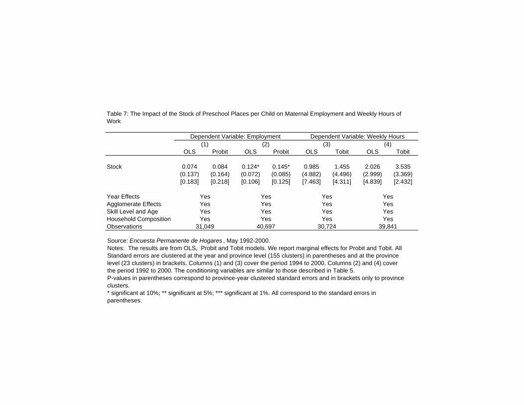
Table 7: The Impact of the Stock of Preschool Places per Child on Maternal Employment and Weekly Hours of Work

OLS Probit OLS Probit OLS Tobit OLS Tobit

Stock 0.074 0.084 0.124* 0.145* 0.985 1.455 2.026 3.535(0.137) (0.164) (0.072) (0.085) (4.882) (4.496) (2.999) (3.369)[0.183] [0.218] [0.106] [0.125] [7.463] [4.311] [4.839] [2.432]

Year EffectsAgglomerate EffectsSkill Level and AgeHousehold CompositionObservations

Dependent Variable: Employment Dependent Variable: Weekly Hours(1) (2) (3) (4)

31,049

YesYesYesYes

40,697

YesYesYesYes

30,724

YesYesYesYes

39,841

YesYesYesYes

Source: Encuesta Permanente de Hogares , May 1992-2000.Notes: The results are from OLS, Probit and Tobit models. We report marginal effects for Probit and Tobit. All Standard errors are clustered at the year and province level (155 clusters) in parentheses and at the province level (23 clusters) in brackets. Columns (1) and (3) cover the period 1994 to 2000. Columns (2) and (4) cover the period 1992 to 2000. The conditioning variables are similar to those described in Table 5. P-values in parentheses correspond to province-year clustered standard errors and in brackets only to province clusters.* significant at 10%; ** significant at 5%; *** significant at 1%. All correspond to the standard errors in parentheses.

Table 8: The Impact of the Stock of Preschool Places per Child on Maternal Employment.Differences by Household Composition

OLS Probit OLS Probit

Stock x Spouse Present 0.125* 0.148*(0.071) (0.085)[0.105] [0.125]

Stock x Spouse Not Present 0.116 0.114(0.129) (0.146)[0.170] [0.196]

Stock x No Children less than 3 0.164** 0.194**(0.082) (0.095)[0.108] [0.128]

Stock x Some Children less than 3 0.068 0.065(0.073) (0.089)[0.121] [0.146]

P-value of F-test for Equality of Treatment Effects (0.9340) (0.7848) (0.1265) (0.0909)[0.9460] [0.8528] [0.2646] [0.2165]

Year Effects Yes Yes Yes YesAgglomerate Effects Yes Yes Yes YesSkill Level and Age Yes Yes Yes YesHousehold Composition Yes Yes Yes YesObservations 40,967 40,967 40,967 40,967

Dependent Variable: Employment(1) (2)

Source: Encuesta Permanente de Hogares, May 1992-2000.Notes: The results are from OLS and Probit. We report marginal effects for Probit. Robust standard errors clustered at the year and province level (155 clusters) in parentheses and at the province level (23 clusters) in brackets. The conditioning variables are similar to those described in Table 5. P-values in parentheses correspond to province-year clustered standard errors and in brackets only to province clusters.* significant at 10%; ** significant at 5%; *** significant at 1%. All correspond to the standard errors in parentheses.