Sampling Methods for How to track many INTERACTING targets ...
14
1 Sampling Methods for Bayesian Inference A Tutorial Frank Dellaert Motivation How to track many INTERACTING targets ? Results: MCMC Dancers, q=10, n=500
Transcript of Sampling Methods for How to track many INTERACTING targets ...

1
Sampling Methods forBayesian Inference
A Tutorial
Frank Dellaert
MotivationHow to track many INTERACTING targets ?
Results: MCMC Dancers, q=10, n=500

2
Probabilistic Topological Maps Results
Real-Time Urban Reconstruction•4D Atlanta, only real time, multiple cameras ☺•Large scale SFM: closing the loop
Current Main Effort: 4D Atlanta
Bayesian paradigm is a useful tool toRepresent knowledgePerform inference
Sampling is a nice way to implement the Bayesian paradigm, e.g. CondensationMarkov chain Monte Carlo methods are a nice way to implement sampling
Goals ReferencesNeal, Probabilistic Inference using MCMC MethodsSmith & Gelfand, Bayesian Statistics Without TearsMacKay, Introduction to MC MethodsGilks et al, Introducing MCMCGilks et al, MCMC in Practice

3
Probability of Robot Location
P(Robot Location)
X
Y
State space = 2D, infinite #states
Density RepresentationGaussian centered around mean x,yMixture of GaussiansFinite element i.e. histogram
Larger spaces -> We have a problem !
Sampling as Representation
P(Robot Location)
X
Y
Sampling Advantages
Arbitrary densitiesMemory = O(#samples)Only in “Typical Set”Great visualization tool !
minus: Approximate
How to Sample ?Target Density P(x)Assumption: we can evaluate P(x) up to an arbitrary multiplicative constant
Why can’t we just sample from P(x) ??
How to Sample ?Numerical Recipes in C, Chapter 7Transformation method: Gaussians etc…Rejection samplingImportance samplingMarkov chain Monte Carlo

4
Rejection Sampling
Target Density PProposal Density Q
P and Q need only be known up to a factor: P* and Q*
must exist c such that cQ*>=P* for all x
The Good…
9% Rejection Rate
…the Bad…
50% Rejection Rate
…and the Ugly.
70% Rejection Rate
Mean and Variance of a Sample
Mean
Variance (1D)
Monte Carlo Expected Value
αExpected angle = 30o

5
Monte Carlo Estimates (General)Estimate expectation of any function f:
Bayes Law
Data = Z
Belief before = P(x) Belief after = P(x|Z)
model P(Z|x)
Prior Distributionof x
Posterior Distributionof x given Z
Likelihoodof x given Z
P(x|Z) ~ P(Z|x)P(x)
Inference by Rejection Sampling
P(measured_angle|x,y) = N(predicted_angle,3 degrees)
Prior(x,y)Posterior(x,y|measured_angle=20o)
Importance SamplingGood Proposal Density would be: prior !Problem:
No guaranteed c s.t. c P(x)>=P(x|z) for all x
Idea:sample from P(x)give each sample x(r) a importance weight equal to P(Z|x (r))
Example Importance Sampling
{x(r),y(r)~Prior(x,y), wr=P(Z|x(r),y(r)) }
Importance Sampling (general)
Sample x(r) from Q*wr = P*(x(r))/Q*(x(r))

6
Important ExpectationsAny expectation using weighted average:
Particle Filtering
1D Robot Localization
Prior P(X)
LikelihoodL(X;Z)
PosteriorP(X|Z)
Importance SamplingHistogram approach does not scaleMonte Carlo ApproximationSample from P(X|Z) by:
sample from prior P(x)weight each sample x(r) using an importance weightequal to likelihood L(x (r);Z)
1D Importance Sampling Particle Filter
π(3)π(1)π(2)
= Recursive Importance Sampling w modeled dynamics
First appeared in 70’s, re-discovered by Kitagawa, Isard, …
7
3D Particle filter for robot pose:Monte Carlo Localization
Dellaert, Fox & Thrun ICRA 99
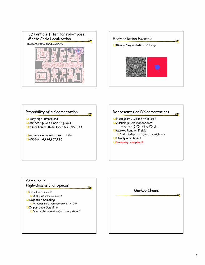
Segmentation ExampleBinary Segmentation of image
Probability of a SegmentationVery high-dimensional256*256 pixels = 65536 pixelsDimension of state space N = 65536 !!!!
# binary segmentations = finite ! 655362 = 4,294,967,296
Representation P(Segmentation)Histogram ? I don’t think so !Assume pixels independent
P(x1x2x2...)=P(x1)P(x2)P(x3)...Markov Random Fields
Pixel is independent given its neighborsClearly a problem !Giveaway: samples !!!
Sampling inHigh-dimensional Spaces
Exact schemes ?If only we were so lucky !
Rejection SamplingRejection rate increase with N -> 100%
Importance SamplingSame problem: vast majority weights -> 0
Markov Chains

8
A simple Markov chain
K= [
0.1 0.5 0.6
0.6 0.2 0.3
0.3 0.3 0.1
]
X1
X3 X2
0.6
0.1
0.3
0.2
0.5
0.3
0.3
0.6
0.1
Stationary Distribution
q0q1 = K q0q2 = K q1 = K2 q0q3 = K q2 = K2 q1 = K3 q0
q10 = K q9 = … K10 q0
[1 0 0] [0 1 0] [0 0 1]
The Web as a Markov Chain
www.yahoo.com
Where do we end up if we click hyperlinks randomly ?
Answer: stationary distribution !
Eigen-analysisK =
0.1000 0.5000 0.6000
0.6000 0.2000 0.3000
0.3000 0.3000 0.1000
E =
0.6396 0.7071 -0.2673
0.6396 -0.7071 0.8018
0.4264 0.0000 -0.5345
D =
1.0000 0 0
0 -0.4000 0
0 0 -0.2000
KE = ED
Eigenvalue v1 always 1
Stationary = e1/sum(e1)i.e. Kp = p
Eigen-analysise1 e2 e3 q
qn=Kn q0 = E Dn c
= p + c2 v2n e2 + c3 v3
n e3+…
Google Pagerank
www.yahoo.com
Pagerank == First Eigenvector of the Web Graph !
Computation assumes a 15% “random restart” probabilitySergey Brin and Lawrence Page , The anatomy of a large-scale hypertextual {Web} search engine, Computer Networks and ISDN Systems, 1998

9
Markov chain Monte CarloBrilliant Idea!
Published June 1953Top 10 algorithm !
Set up a Markov chainRun the chain until stationaryAll subsequent samples are from stationary distribution
Markov chain Monte CarloIn high-dimensional spaces:
Start at x0~ q0
Propose a move K(xt+1|xt)
K never stored as a big matrix ☺K as a function/search operator
Example
How do get the right chain ?Detailed balance:
K(y|x) p(x) = K(x|y) p(y)
0.5 * 9/14 = 0.9 * 5/14
X4 X5
0.10.9
0.5
0.5
Reject fraction of moves !Detailed balance:
K(y|x) 1/3 = K(x|y) 2/3
0.5 * 1/3 = a * 0.9 * 2/3a = 0.5 * 1/3 / (0.9 * 2/3)
= 5/18
X4 X5
0.10.9
0.5
0.5
X4 X5
0.750.25
0.5
0.5

10
Metropolis-Hastings Algorithm- pick x(0), then iterate over:1. propose x’ from Q(x’;x(t))2. calculate ratio
3. if a>1 accept x(t+1)=x’ else accept with probability aif rejected: x(t+1)=x(t)
Again !
1. x(0)=10
2. Proposal:x’=x-1 with Pr 0.5x’=x+1 with Pr 0.5
3. Calculate a:a=1 if x’ in [0,20]a=0 if x’=-1 or x’=21
4. Accept if 1, reject if 0
5. Goto 2
1D Robot Localization
Chain started at randomConverges to posterior
Localization Eigenvectors
0.9962
1.0000
Gibbs Sampling- MCMC method that always accepts- Algorithm:
- alternate between x1 and x2
- 1. sample from x1 ~ P(x1|x2)- 2. sample from x2 ~ P(x2|x1)
- Rationale: easy conditional distributions- = Gauss-Seidel of samplers
11
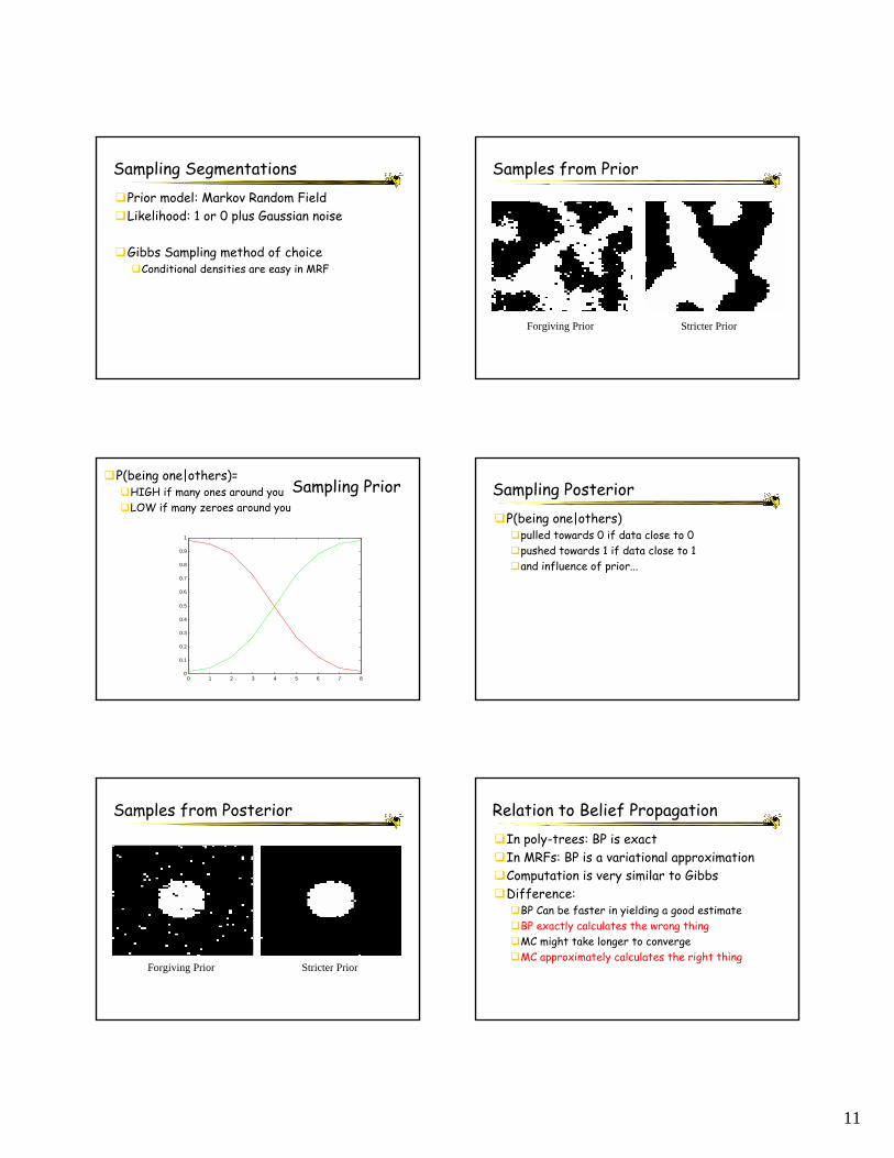
Sampling SegmentationsPrior model: Markov Random FieldLikelihood: 1 or 0 plus Gaussian noise
Gibbs Sampling method of choiceConditional densities are easy in MRF
Samples from Prior
Forgiving Prior Stricter Prior
Sampling PriorP(being one|others)=
HIGH if many ones around youLOW if many zeroes around you
0 1 2 3 4 5 6 7 80
0.1
0.2
0.3
0.4
0.5
0.6
0.7
0.8
0.9
1
Sampling PosteriorP(being one|others)
pulled towards 0 if data close to 0pushed towards 1 if data close to 1and influence of prior...
Samples from Posterior
Forgiving Prior Stricter Prior
Relation to Belief PropagationIn poly-trees: BP is exactIn MRFs: BP is a variational approximationComputation is very similar to GibbsDifference:
BP Can be faster in yielding a good estimateBP exactly calculates the wrong thingMC might take longer to convergeMC approximately calculates the right thing

12
Relation to Belief Propagation Application: Edge Classification
Given vanishing points of a scene, classify each pixel according to vanishing direction
MAP Edge Classifications
Red: VP1 Green: VP2 Blue: VP3 Gray: Other White: Off
Bayesian Model
p(M | G,V) = p(G | M,V) p(M) / ZM = classifications, G = gradient magnitude/direction, V = vanishing points
Prior: p(m)
Likelihood: p(g | m,V)
Independent Prior MRF Prior
m
g
Classifications w/MRF Prior
Gibbs sampling over 4-neighbor lattice w/ clique potentials defined as: A if i=j, B if i <> j
Gibbs Sampling & MRFs
Gibbs sampling approximates posterior distribution over classifications at each site (by iterating and accumulating statistics)
Sample from distribution over labels for one site conditioned on all other sites in its Markov blanket

13
Directional MRF
Give more weight to potentials of neighbors which lie along the vanishing direction of current model
vp
Original Image
Independent Prior MRF Prior
Directional MRF Prior
Bayesian paradigm is a useful tool toRepresent knowledgePerform inference
Sampling is a nice way to implement the Bayesian paradigm, e.g. CondensationMarkov chain Monte Carlo methods are a nice way to implement sampling
Take Home Points !

14
World Knowledge
P(z|x)
z
xSensor Model
Most often analytic expression, can be learned
d
d
Proposal Density Q- Q(x’;x) that depends on x
Step Size and #Samples- Too large: all rejected- Too small: random walk- E[d]=e sqrt(T)- Rule of thumb: T>=(L/e)2
- Bummer: just a lower bound
Discussion Example- e=1- L=20- T>=400- Moral: avoid random walks
MCMC in high dimensions- e=smin- L=smax- T=(smax/smin)2
- Good news: no curse in N- bad news: quadratic dependence


![Phytochromes and Phytochrome Interacting Factors1[OPEN] · Update on Phytochromes and Phytochrome Interacting Factors Phytochromes and Phytochrome Interacting Factors1[OPEN] Vinh](https://static.fdocuments.net/doc/165x107/5e9224c5cbd0a85457462c45/phytochromes-and-phytochrome-interacting-factors1open-update-on-phytochromes-and.jpg)