Sampling Directed Graphs with Random Walks · Sampling Directed Graphs with Random Walks UMass...
11
Sampling Directed Graphs with Random Walks UMass CMPSCI Technical Report UMCS-2011-031 Bruno Ribeiro 1 , Pinghui Wang 2 , Fabricio Murai 1 , and Don Towsley 1 1 Computer Science Department 2 State Key Lab for Manufacturing Systems University of Massachusetts Xi’an Jiaotong University Amherst, MA, 01003 Xi’an P.R.China {ribeiro, fabricio, towsley}@cs.umass.edu [email protected] Abstract—Despite recent efforts to characterize complex net- works such as citation graphs or online social networks (OSNs), little attention has been given to developing tools that can be used to characterize directed graphs in the wild, where no pre- processed data is available. The presence of hidden incoming edges but observable outgoing edges poses a challenge to char- acterize large directed graphs through crawling. Unless we can crawl the entire graph or the directed graph edges are highly symmetrical, hidden incoming edges induce unknown biases in the sampled nodes. In this work we propose a random walk sampling algorithm that is less prone these biases. The driving principle behind our random walk is to construct, in real-time, an undirected graph from the directed graph in a way that is consistent with the sample path followed by the algorithm walking on either graph. We also study outdegree and indegree distribution estimation. Out-degrees are visible to the walker while indegrees are hidden (latent). This makes for strikingly different estimation accuracies of in- and outdegree distributions. Our algorithm accurately estimates outdegree distributions of a variety of real world graphs while we show that, in the same sce- narios, no algorithm can accurately estimate unbiased indegree distributions unless the directed graph is highly symmetrical. I. I NTRODUCTION Despite recent efforts to characterize complex networks such as citation graphs or online social networks (OSNs), little attention has been given to developing tools that can be used to characterize directed graphs in the wild, where no pre- processed data is available. A network is said to be directed when the relationships between its agents (users or profiles) may not be reciprocated. For instance, a Wikipedia [19] entry about Columbia Records cites Thomas Edison but Thomas Edison’s entry makes no reference to Columbia Records. The presence of hidden incoming edges but observable outgoing edges makes characterizing large directed graphs through crawling a challenge. An edge b → a is a hidden incoming edge of node a if b → a can only be observed from node b. For instance, in our earlier Wikipedia example about Columbia Records and Thomas Edison we cannot observe the edge “Columbia Records” → “Thomas Edison” from Thomas Edison’s wiki entry (but this edge is observable if we access Columbia Records’s wiki entry). Unless we can crawl the entire graph, hidden incoming edges induce unknown biases in the sampled nodes. Moreover, there may not even be a directed path from a given node to all other nodes. Graphs with hidden outgoing edges but observ- able incoming edges exhibit essentially the same problem. In this work we propose a random walk sampling algorithm that does not suffer from unknown sampling biases when partially crawling directed graphs with hidden incoming edges. More importantly, we present a method to unbias the samples. Our random walk algorithm resorts to two main principles to achieve unbiased samples: • In real-time we construct an undirected graph using the directed nodes that are sampled by the random walker on the directed graph. The undirected graph role is to guarantee that at the end of the sampling process we can approximate the probability of sampling a node, even though incoming edges are not observed. The random walk proceeds in a way that the sample path of walking on the directed graph is consistent with the sample path followed by the algorithm when walking on the constructed undirected graph. Knowing the sampling probability of a node allows us to unbias the samples. • A very limited amount of uniformly sampled nodes (less than 0.01 of all sampled nodes) to guarantee that different parts of the directed graph are explored. Contributions Our work makes two main contributions: • Directed Unbiased Random Walk (DURW): Our random walk algorithm accurately estimates characteristics of large directed graphs through sampling. • In-degree Distribution Estimation: We show that no unbi- ased estimator can accurately obtain the indegree distribu- tion (recall indegrees are latent variables in the directed graph) of the datasets used in this work from sampled edges unless a large fraction of the graph is sampled or the graph is highly symmetric. This result is surprising as the average indegree and average outdegree are identical and the outdegree distribution can be accurately characterized. Outline The rest of the paper is organized as follows. Section II presents the graph model and some definitions used throughout this work. Section III presents our DURW algorithm and estimators. Section IV our outdegree distribution estimation simulation results on real world graphs. Section V presents an application of DURW on the Wikipedia network. Section VI shows that indegree distribution estimation is inaccurate unless
Transcript of Sampling Directed Graphs with Random Walks · Sampling Directed Graphs with Random Walks UMass...

Sampling Directed Graphs with Random Walks
UMass CMPSCI Technical Report UMCS-2011-031
Bruno Ribeiro1, Pinghui Wang2, Fabricio Murai1, and Don Towsley1
1Computer Science Department 2State Key Lab for Manufacturing Systems
University of Massachusetts Xi’an Jiaotong University
Amherst, MA, 01003 Xi’an P.R.China
{ribeiro, fabricio, towsley}@cs.umass.edu [email protected]
Abstract—Despite recent efforts to characterize complex net-works such as citation graphs or online social networks (OSNs),little attention has been given to developing tools that can beused to characterize directed graphs in the wild, where no pre-processed data is available. The presence of hidden incomingedges but observable outgoing edges poses a challenge to char-acterize large directed graphs through crawling. Unless we cancrawl the entire graph or the directed graph edges are highlysymmetrical, hidden incoming edges induce unknown biases inthe sampled nodes. In this work we propose a random walksampling algorithm that is less prone these biases. The drivingprinciple behind our random walk is to construct, in real-time,an undirected graph from the directed graph in a way thatis consistent with the sample path followed by the algorithmwalking on either graph. We also study outdegree and indegreedistribution estimation. Out-degrees are visible to the walkerwhile indegrees are hidden (latent). This makes for strikinglydifferent estimation accuracies of in- and outdegree distributions.Our algorithm accurately estimates outdegree distributions of avariety of real world graphs while we show that, in the same sce-narios, no algorithm can accurately estimate unbiased indegreedistributions unless the directed graph is highly symmetrical.
I. INTRODUCTION
Despite recent efforts to characterize complex networks
such as citation graphs or online social networks (OSNs), little
attention has been given to developing tools that can be used
to characterize directed graphs in the wild, where no pre-
processed data is available. A network is said to be directed
when the relationships between its agents (users or profiles)
may not be reciprocated. For instance, a Wikipedia [19] entry
about Columbia Records cites Thomas Edison but Thomas
Edison’s entry makes no reference to Columbia Records.
The presence of hidden incoming edges but observable
outgoing edges makes characterizing large directed graphs
through crawling a challenge. An edge b → a is a hidden
incoming edge of node a if b → a can only be observed from
node b. For instance, in our earlier Wikipedia example about
Columbia Records and Thomas Edison we cannot observe the
edge “Columbia Records” → “Thomas Edison” from Thomas
Edison’s wiki entry (but this edge is observable if we access
Columbia Records’s wiki entry).
Unless we can crawl the entire graph, hidden incoming
edges induce unknown biases in the sampled nodes. Moreover,
there may not even be a directed path from a given node to all
other nodes. Graphs with hidden outgoing edges but observ-
able incoming edges exhibit essentially the same problem.
In this work we propose a random walk sampling algorithm
that does not suffer from unknown sampling biases when
partially crawling directed graphs with hidden incoming edges.
More importantly, we present a method to unbias the samples.
Our random walk algorithm resorts to two main principles to
achieve unbiased samples:
• In real-time we construct an undirected graph using the
directed nodes that are sampled by the random walker
on the directed graph. The undirected graph role is to
guarantee that at the end of the sampling process we
can approximate the probability of sampling a node, even
though incoming edges are not observed. The random
walk proceeds in a way that the sample path of walking
on the directed graph is consistent with the sample path
followed by the algorithm when walking on the constructed
undirected graph. Knowing the sampling probability of a
node allows us to unbias the samples.
• A very limited amount of uniformly sampled nodes (less
than 0.01 of all sampled nodes) to guarantee that different
parts of the directed graph are explored.
Contributions
Our work makes two main contributions:
• Directed Unbiased Random Walk (DURW): Our random
walk algorithm accurately estimates characteristics of large
directed graphs through sampling.
• In-degree Distribution Estimation: We show that no unbi-
ased estimator can accurately obtain the indegree distribu-
tion (recall indegrees are latent variables in the directed
graph) of the datasets used in this work from sampled
edges unless a large fraction of the graph is sampled or the
graph is highly symmetric. This result is surprising as the
average indegree and average outdegree are identical and
the outdegree distribution can be accurately characterized.
Outline
The rest of the paper is organized as follows. Section II
presents the graph model and some definitions used throughout
this work. Section III presents our DURW algorithm and
estimators. Section IV our outdegree distribution estimation
simulation results on real world graphs. Section V presents an
application of DURW on the Wikipedia network. Section VI
shows that indegree distribution estimation is inaccurate unless

most of the graph is sampled (even with side information).
Section VII reviews the related work. Finally, Section VIII
presents our conclusions and future work.
II. DEFINITIONS AND PROBLEM FORMULATION
Let Gd = (V,Ed) be a directed graph, where V is the set of
nodes and Ed is the set of edges. Let o(v) denote the number
of edges out of node v ∈ V (outdegree) and i(v) denote the
number of edges into node v ∈ V (indegree). We seek to
obtain both the outdegree distribution φ = (φ0, φ1, ..., φR)and the indegree distribution θ = (θ0, θ1, ..., θW ), where φl is
the fraction of nodes with outdegree l, θj is the fraction of
nodes with indegree j, R is the largest outdegree, and W is
the largest indegree.
The degree distribution of a large undirected graph can be
estimated using random walks (RW) [8], [12], [14]. But these
RW methods cannot be readily applied to directed graphs with
hidden incoming edges, which is the case of a number of
interesting directed networks, e.g., the WWW, Wikipedia, and
Flickr.
To address these problems, we build a random walk with
jumps under the assumption that nodes can be sampled uni-
formly at random from Gd (something not feasible for the
WWW graph but possible for Wikipedia and Flickr). But why
perform a random walk if we can sample nodes uniformly?
There are two reasons for that: (1) Random walk is more
efficient in networks where uniform node sampling is costly
(e.g., Flickr). We denote the cost of random node sampling
c. In networks were users have numeric IDs, the cost of
uniformly sampling comes from the fact that the ID space
is sparsely populated [5], [6], [13] and a number of uniformly
generated ID values are invalid. In these networks c is the
average number of IDs queried until one valid ID is obtained.
For instance, in the case of MySpace and Flickr, we estimate
these costs to be c = 10 [13] and c = 77 (refer to our technical
report [15]), respectively. (2) A random walk can better
characterize highly connected nodes than uniform sampling as
random walks are biased to sample highly connected nodes.
This bias can be later corrected, giving us smaller estimation
errors for the characteristics of highly connected nodes.
III. SAMPLING DIRECTED GRAPHS WITH DURWS
Estimating characteristics of undirected graphs with random
walks (RWs) is the subject of a number of recent works [12],
[14], [16]. RW estimation methods presented in the literature
require that ∀u, v ∈ V , the probability of eventually reaching
u given that the walker is in v be non-zero. However, over
a directed graph with hidden incoming edges this may not
be true. For instance, consider a node v ∈ V that has one
outgoing edge but no incoming edges. If the random walker
does not start at v then v is not visited by the walker (as the
outgoing edge of v is a hidden incoming edge if some other
node). On the other hand, a node u ∈ V with no outgoing
edges becomes a sink to the random walker.
A natural way to deal with the unreachability of nodes is
to perform random jumps within the random walk, just like
the PageRank algorithm [4]. The PageRank walker at node vjumps to a uniformly chosen node in the graph with probability
α; and with probability (1−α) the walker performs a RW step
(i.e., follows an edge chosen uniformly at random from the
set of outgoing edges of v). Unfortunately, next we see that
PageRank is not well suited to characterize directed graphs.
A. The case against PageRank sampling
Unfortunately, PageRank does not allow us to accurately
estimate graph characteristics, such as the outdegree distribu-
tion, from a sampled subset of the graph. Estimating these
characteristics requires obtaining the steady state distribution
of the RW without exploring the entire graph [14].
s1s2
s3
s4 s5
s6
s7
s1s2
s3
s4 s5
s6G2
s7
G1
Figure 1: PageRank dependence on graph structure: Without
sampling s7 one cannot tell the PageRank sampling probability
of node s1.
In the example of Figure 1 we see that the steady state
distribution of PageRank requires knowing the graph structure.
Consider the two directed graphs, G1 and G2, with 7 nodes
each, as shown in Figure 1. Incoming edges are hidden. Let s1be the starting node of PageRank. Let π(v) denote the steady
state probability that PageRank visits node v, ∀v ∈ V . For
graph G1 π(s1) = 1/7 and for graph G2 π(s1) = α/(7α+6).Thus, the sampling probability of s1 depends on the edges
of the unsampled node s7. The above example shows why
PageRank is not suited to sample large graphs.
B. Directed Unbiased Random Walk (DURW)
Our Directed Unbiased Random Walk (DURW) algorithm
has two parts:
• Backward edge traversals (detailed in Section III-C): We
allow the random walker to traverse known outgoing edges
backwards under certain conditions. For instance, if at the
i-th step the RW is at node si, we allow the random walker
to traverse the edge si−1 → si backwards. However, in
order to avoid large transients the algorithm places some
restriction on which edges can be made undirected.
• Degree-proportional jumps (detailed in Section III-D):
The algorithm performs a jump from node v to an uni-
formly chosen node, ∀v ∈ V , with probability w/(w +deg(v)), where deg(v) is the degree of v in the undirected
graph Gu. Our jumping algorithm is subtle but fundamen-
tally different than other random jump algorithms such as
PageRank.
C. Backward edge traversals
We allow the walker to traverse some outgoing edges
backwards. In general, if we apply this “backward walking”
principle to all outgoing edges in Gd, we can construct an
undirected version of Gd. The undirected version of Gd
allows us to apply the techniques described in Ribeiro and
2

Towsley [14] to estimate the characteristics of Gd such as the
outdegree distribution. However, the degree of a node v in the
final undirected version of Gd is only known after exploring
all edges of Gd. Thus, the above sampling algorithm is not
practical as unbiasing the sampled would require access to the
complete underlying graph (as the probability is a function of
v’s degree [14]).
To avoid this problem our RW interactively builds an
undirected graph Gu. This building process is such that once
a node is visited at the i-th step no additional edges are
added to that node in subsequent steps. Such a restriction fixes
the degree of the nodes visited by the random walker, thus
ensuring that nodes will not keep changing their degrees as
we walk the graph. This is an important feature to reduce the
unknown bias of the random walk transient and thus reducing
estimation errors. Note that the final undirected graph Gu
depends on the sample path taken by the random walker.
Further details of the algorithm can be found in Section III-E.
The above solution addresses the problem of knowing the
degree of a node as soon as the node is sampled. However,
we still do not know the steady state distribution of the RW
when we add random jumps. In what follows we present
an algorithm that allows us to obtain a simple closed-form
solution to the steady state distribution.
D. Degree-proportional jumps
Let Gu = (V,Eu) be an undirected graph. In DURW, the
probability of randomly jumping out of a node v, ∀v ∈ V ,
is w/(w + deg(v)), w > 0 . This modification is based on
a simple observation: let G′ be a weighted undirected graph
formed by adding a node σ to Gu such that σ is connected
to all nodes in V with edges having weight w. All remaining
edges have unitary weight. In a random walk in a weighted
graph walks over an edge with probability proportional to
the edge weight. The steady state probability of visiting a
node v on G′ is (w + deg(v))/(vol(V ) + w|V |), where
vol(V ) =∑
∀u∈V deg(u). Thus, except for the unknown
constant normalization term (vol(V )+w|V |), the steady state
distribution of v is known as we know the degree of v and the
value of parameter w when v is visited by the random walker.
By combining backward edge traversal (Section III-C)
and degree-proportional jumps (Section III-D) we obtain the
DURW algorithm.
E. The DURW algorithm
DURW is a random walk over a weighted undirected
connected graph Gu = (V,Eu), which is built on-the-fly.
The algorithm works as follows. We build an undirected
graph using the underlying directed graph Gd and the ability
to perform random jumps. Let G(i) = (V (i), E(i)) be the
constructed undirected “graph” at DURW step i, where V (i)
is the node set and E(i) is the edge set. We call G(i) a “graph”
because we allow E(i) to have edges of nodes that are not in
V (i). Denote Gu ≡ limi→∞ G(i). In what follows we describe
the construction of G(i).
Let v ∈ V be the initial node in the random walk. Let N (v)denote the outgoing edges of v in Gd and let node σ denote
a virtual node that represents a random jump. We initialize
G(1) = ({s1}, E(1)), where E(1) = N (s1) ∪ {(u, σ) : ∀u ∈V }, where {(u, σ) : ∀u ∈ V } is the set of all undirected
virtual edges to virtual node σ (this construct of adding edges
to σ is introduced to simplify our exposition, in practice we
do not need to add virtual edges to σ). Note that we allow
self loops created when σ = s1. The random walker proceeds
as follows.
We start with i = 1; at step i the random walker is at node
si. Let
W (u, v) =
{
w if u = σ or v = σ
1 otherwise
denote the weight of edge (u, v), ∀(u, v) ∈ E(i), i = 1, 2, . . . .The next node, si+1, is selected from E(i) with probability
W (si, si+1)/∑
∀(si,v)∈E(i) W (si, v). Upon selecting si+1 we
update G(i+1) = (V (i) ∪ {si+1}, E(i+1)), where
E(i+1) = E(i) ∪ N ′(si+1) , (1)
and
N ′(si+1) = {(si+1, v) : ∀(si+1, v) ∈ N (si+1) s.t. v 6∈ V (i)}is the set of all nodes (u, v) in N (si+1) where node v is not
already in V (i). Note that N ′(si+1) ⊆ N (si+1). By using
N ′(si+1) instead of N (si+1) in equation (1) we guarantee
that no nodes in V (i) change their degrees, i.e., ∀v ∈ V (i) the
degree of v in G(i) is also the degree of v in Gu. Thus, we
comply with the requirement presented in Section III-C that
once a node v, ∀v ∈ V , is visited by the RW no edges can be
added to the graph with v as an endpoint.
The edges in G(i), i = 1, 2, . . . , that connect all nodes to
the virtual node σ can be easily emulated with uniform node
sampling.
Space complexity: The space required to store G(i) is
O(|E|), where |E| is the number of edges in the graph.
F. Out-degree Distribution Estimator
In this section we use the nodes visited (sampled) by our
DURW algorithm to estimate the outdegree distribution. The
estimator presented in this section can be easily extended
to obtain the distribution of node labels, as detailed in Sec-
tion III-G.
Let si denote the i-th edge visited by DURW, i = 1, . . . , n,n ≥ B. Let φj be the fraction of nodes with outdegree j in
Gd. Let π(v) be the steady state probability of sampling node
v in Gu, ∀v ∈ V . The outdegree distribution can be estimated
as
φj =1
B
B∑
i=1
hj(si)
π(si), j = 0, 1, . . . (2)
where hj(v) is the indicator function
hj(v) =
{
1 if the outdegree of v in Gd is j ,
0 otherwise
and π(si) is an estimate of π(si): π(si) = (w + deg(si))S .
3

Here deg(v) is the degree of v in G(∞) and
S =1
B
B∑
i=1
1
w + deg(si).
The following theorem shows that π(si) is asymptotically
unbiased.
Theorem 3.1: π(si) is an asymptotically unbiased estimator
of π(si).
Proof: To show that π(si) an asymptotically unbiased we
invoke Theorem 4.1 of Ribeiro and Towsley [14], yielding
limB→∞ S = |V |/(|E(∞)| + |V |w) almost surely. Thus,
limB→∞ π(si) = π(si) almost surely. Taking the expectation
of Equation (2) in the limit B → ∞ yields E[limB→∞ φj ] =φj , which concludes our proof.
G. Estimating other metrics
In a more general setting we seek to estimate the distribution
obtained by the function
hj(v) =
{
1 node v is labeled j,0 otherwise.
(3)
where labels can indicate any characteristics of the nodes.
In order to estimate the fraction of nodes with label j,we plug the values hj(si), si = 1, . . . , n, n ≥ B into
equation (2). Here π is computed in the same way as before
and E[limB→∞ φj ] = φj , still holds.
Now that we have an asymptotically unbiased estimators it
is left to test the accuracy of DURW in a variety of real world
graphs.
IV. EXPERIMENTAL RESULTS
This section compares the outdegree distribution estimates
obtained by our algorithm (DURW) against the estimates
obtained by the random walk algorithm of Bar-Yossef et al. [3]
(presented in Section VII) and independent uniform node
sampling (UNI). Our experiments are performed on a variety
of real world graph datasets. The statistics of these datasets
are summarized in Table I.
We now describe each dataset. Flickr, LiverJournal, and
YouTube are popular photosharing, blog, and video sharing
websites, respectively. In these websites a user (node) can
subscribe to other user (nodes) updates forming a directed
edge. Wikipedia is a free encyclopedia written collaboratively
by volunteers. Each registered user has a talk page, that she
and other users can edit in order to communicate and discuss
updates to various articles on Wikipedia. Nodes in the Wiki-
Talk dataset represent Wikipedia users and a directed edge
from node u to node v represents that user u edited a talk
page of user v at least once. The Web-Google dataset was
released in 2002 by Google as a part of Google Programming
Contest, where nodes represent web pages and directed edges
represent hyperlinks between them [1]. Further details of the
Flickr, LiverJournal, and YouTube datasets can be found in
Mislove et al. [11].
Table I: Overview of directed graph datasets used in our
simulations.
Graph # nodes # edges E[out-deg] symmetry Type
Flickr [11] 1,715,255 22,613,981 18.1 0.38 OSN
YouTube [11] 1,138,499 4,945,382. 5.3 0.21 OSN
LiveJournal [11] 5,204,176 77,402,652 18.7 0.27 OSN
Wiki-Talk [2] 2,394,385 5,021,410 3.9 0.86 usr talk
Web-Google [1] 875,713 5,105,039 9.87 0.69 Web
Error Metric
Before we proceed with our results we need to introduce the
error metric used to compare the different sampling methods
we want to test. Our primary metric of interest is the outdegree
distribution. We chose this metric because the outdegree
distribution is a metric that is present in all of our datasets.
Let
NMSE(φj) =
√
E[(φj − φj)2]
φj
, j = 1, 2, . . . ,
be a metric that measures the relative error of the estimate φj
with respect to its true value φj . Note that our metric uses
the relative error. Thus, when φj is small, we consider
values as large as NMSE(φj) = 1 to be acceptable. Let cdenote the cost of UNI which is also the cost of a random
jump (the average number of IDs queried until one valid ID
is obtained). For instance, Flickr has a random node sampling
cost of c = 77 (as observed in the experiments presented
in [15]). Let B denote the sampling budget (when c = 1, B is
the number of distinct sampled nodes). Because we create an
undirected graph on the side, multiple visits to the same node
counts as just one unit of the sampling budget. Also, before
proceeding to our results, it is important to note that in DURW
the probability of performing a random jump increases with w(such that in the limit w → ∞ DURW is equivalent to UNI).
Results
The first simulation results are presented in Figures 2
to 4d. Figure 2 shows three sample paths with estimates of
φ1000 (y-axis) using DURW (using random jump weights
w ∈ {0.1, 1, 10}) and UNI. The x-axis shows the number of
samples (in log scale). These results were obtained using the
Youtube dataset with independent sampling cost c = 1. Thechoice of φ1000 is arbitrary; later we investigate estimation er-
rors of all degrees. Note that none of the three runs of UNI can
find a single node with outdegree 1000 until almost 200, 000nodes have been sampled. On the other hand, our DURW
algorithm quickly finds at least one node with outdegree 1000.Moreover, DURW has consistently smaller estimation errors
than UNI throughout most of the sample paths.
Figures 3 to 4d show estimates of the NMSE in log scale
(over 1000 runs) of DURW for all outdegrees in the graph
over different datasets. In these simulations we compare the
NMSE of DURW with the NMSE of the Metropolis-Hastings
algorithm of Bar-Yossef et al. [3] and the NMSE of uniform
random sampling (UNI). In all first five scenarios we sample
10% of the graph. The DURW random jump weight and cost
4

are w = 10 and c = 10, respectively. Figures 3, 4a, 4b, 4c, 4dshow the NMSE for the Youtube, Wiki-Talk, Flickr, Livejour-
nal, and Web-Google datasets, respectively.
We find that DURW obtains accurate estimates over all
datasets, recalling that we consider NMSE(φj) ≤ 1 to be
an accurate estimator if φj is small, as the NMSE measures
the relative error of φj when compared to the true value
φj . DURW outperforms all other methods w.r.t. the accuracy
when estimating the fraction of nodes with large outdegrees,
often by a factor of one order of magnitude.Moreover, DURW
is significantly more accurate than Bar-Yossef et al. [3] over
almost all outdegrees values. In the Youtube, Wiki-Talk, Flickr,
and Livejournal datasets the value of φj obtained with DURW
for large outdegrees is up to two orders of magnitude more
accurate than Bar-Yossef et al. [3]. DURW is also consistently
more accurate over most outdegrees than UNI for the Youtube,
Wiki-Talk and Flickr datasets. DURW is also more accurate
than UNI in the Livejournal and Web-Google datasets for
large outdegrees (outdegrees larger than 50 in Livejournal and
outdegrees larger than 30 in Web-Google).
In Figures 3 to 4d we note that UNI is sometimes slightly
better than DURW for low degrees, but not by much. This
is because DURW is biased towards sampling nodes with
high outdegrees and indegrees (these nodes tend to have high
degrees in our constructed undirected graph). Thus, DURW
tends to sample nodes with few outgoing edges less frequently
than UNI, sometimes causing larger estimation errors for these
small outdegree nodes. As we see later, increasing the DURW
jump weight parameter w reduces the estimation error for
small outdegrees at the cost of increasing the error of larger
outdegrees.
1,000 10,000 100,000 0.5|V|0
1
2
3
4
5
6x 10
−6
number of distinct vertices sampled
DURW, w=0.01
DURW, w=1
DURW, w=10
UNI
φ1000
Figure 2: (YouTube) True value of φ1000 = 1.8×10⁻⁶ shown
in the black solid line. Y-axis: Estimated φ1000 (DURW with
w ∈ 0.1, 1, 10 and UNI). X-axis: Number of samples in log-
scale. DURW is consistently better than UNI.
A. Varying DURW Parameters
In what follows we study the impact of the DURW parame-
ters on the accuracy of the estimates. Figure 5 shows the results
of varying the random jump weight, w, while keeping the
random jump cost c = 10 and the sampling budgetB = 0.1|V |fixed. The DURW parameter w controls the trade-off between
the error for estimating small and large outdegrees. As wincreases, the estimation error for large outdegrees increases
while the error of small outdegrees decreases. Conversely,
as w decreases the opposite happens, the estimation error of
100
101
102
103
104
105
10−2
10−1
100
101
102
out−degree
NM
SE
DURW (our algorithm)
UNI
Bar−Yossef et al.
Figure 3: (YouTube) NMSE of DURW with B0.1|V |, w = 10,and c = 10 compared with UNI.
100
101
102
103
104
105
10−2
10−1
100
101
102
out−degree
NM
SE
DURW (our algorithm)
UNI
Bar−Yossef et al.
(a) Wiki-Talk
100
101
102
103
104
105
10−3
10−2
10−1
100
101
102
out−degree
NM
SE
DURW (our algorithm)
UNI
Bar−Yossef et al.
(b) Flickr
100
101
102
103
104
10−3
10−2
10−1
100
101
102
out−degree
NM
SE
DURW (our algorithm)
UNI
Bar−Yossef et al.
(c) LiveJournal
100
101
102
103
10−2
10−1
100
101
102
out−degree
NM
SE
DURW (our algorithm)
UNI
Bar−Yossef et al.
(d) Web-Google
Figure 4: NMSE of DURW with B = 0.1|V |, w = 10, andc = 10 compared with UNI.
large outdegrees decreases while the error for small degrees
increase. This is expected, as when w increases the DURW
algorithm performs random jumps often and, thus, mimics
uniform sampling (UNI), sampling small outdegrees nodes
more often.
In the next set of simulations we look at the im-
pact of the sampling budget, B, on the NMSE. Figure 6
presents the NMSE of Youtube for sampling budgets B ∈{0.01|V |, 0.1|V |, 0.2|V |} with c = 10 and w = 10. We
observe that the error of sampling B nodes is roughly pro-
portional to 1/√B. For instance, in Figure 6 we see that a
one order of magnitude increase in B roughly decreases the
error by 1/√10.
As DURW can perform random jumps, we also study
the impact of the cost of these jumps over the accuracy
of the estimates. The cost of a jump is measured by the
5

amount of “sampling budget” (queries) required to perform
the jump. On some social networks, such as MySpace and
Flickr, a number of queries is needed to sample a node
uniformly at random. For instance, on Flickr random jumps
are performed by querying randomly generating user IDs. The
average number of random IDs queried until one valid ID is
obtained is 77 to 1 (see our technical report [15]). The cost of
jumps effectively reduces the number of total nodes that can be
sampled, and, thus, increases the NMSE. Figure 7a shows the
NMSE of Youtube with c ∈ {1, 10, 77} and constant values
B = 0.1|V | and w = 10. Unsurprisingly, we observe that
the estimation error of the outdegree distribution tail increases
with c. As decreasing w decreases the frequency of jumps,
which reduces the impact of parameter c the NMSE error.
To better understand this relationship, we repeat the above
experiment (Figure 7a) with less frequent jumps w = 1. InFigure 7b we plot the NMSE of the DURW algorithm with
different values of c ∈ {1, 10, 77} and keeping w = 1 constant.Comparing Figures 7a and 7b we see that a smaller w can
significantly lessen the negative impact of higher jump costs
on the accuracy of the estimator.
100
101
102
103
104
105
10−2
10−1
100
101
102
103
out−degree
NMSE
DURW (our algorithm), w=0.01
DURW (our algorithm), w=1
DURW (our algorithm), w=10
DURW (our algorithm), w=1000
UNI
Figure 5: (Youtube) NMSE of DURW with w ∈{0.01, 1, 10, 1000} against the NMSE of UNI, c = 10 and
B = 0.1|V |.
100
101
102
103
104
105
10−2
10−1
100
101
out−degree
NMSE
B=0.01|V|
B=0.1|V|
B=0.2|V|
Figure 6: (Youtube) NMSE of DURW with B ∈{0.01|V |, 0.1|V |, 0.2|V |}, c = 10 and w = 10.
V. APPLICATIONS
In this section we describe some experiments performed to
estimate other metrics evaluated at the Wikipedia network. As
opposed to the results presented in the previous section, which
are based on datasets, we now use a DURW to crawl the graph
in an online fashion.
These metrics are interesting if measured online: (1) the
time between two consecutive article (node) revisions and (2)
100
101
102
103
104
105
10−2
10−1
100
101
out−degree
NM
SE
c=1
c=10
c=77
(a) w = 10
100
101
102
103
104
105
10−2
10−1
100
101
out−degree
NM
SE
c=1
c=10
c=77
(b) w = 1
Figure 7: (Youtube) NMSE of DURW with c ∈ {1, 10, 77},B = 0.1|V | and w = {1, 10}.
the distribution of the number of revisions in the last 7 days,
classified by the outdegree of the node (article). But why do
we want to sample Wikipedia revisions using DURW? Articles
that point to several other articles are likely to suffer more
revisions than nodes with almost no references. As DURW
can accurately estimate metrics of nodes with high outdegrees
(see Section IV), DURW is well equipped to estimate revision-
related metrics.
Wikipedia provides a query API that can be used to obtain
information from an node such as the categories to which it be-
longs, its revision timestamps (timestamps marking when the
node was changed) and the content itself, which includes the
text describing the node and links to other Wikipedia nodes.
We implemented a crawler that uses this query API to perform
a DURW random walk on the Wikipedia graph. Our DURW
crawler collected 60,000 Wikipedia nodes (approximately 2%of the entire Wikipedia database) over the course of two days
(from 07/27/2011 5pm until 07/29/2011 5pm).
Wikipedia API can also retrieve a randomly sampled page
from its collection of nodes (two queries are needed to obtain
one page). We set the DURW jump weight to w = 0.1,allowing the walker to perform some random jumps while
preserving most of the random walk characteristic of sampling
high degree nodes. We are interested in sampling high degree
nodes well because these nodes, although rare, are likely to
be the ones that are edited more frequently.
When an node is visited, the crawler also gathers measures
of interest such as the outdegree and the times of the 500 most
recent revisions. For conciseness, we omit the results regarding
the outdegree (see Section III-G for a description of how to
estimate the outdegree distribution). In particular, the metrics
we obtain for a node v in our DURW include:
• X(v): number of revisions of v created in date d ∈ [R(v)−7 days, R(v)], and
• Y (v): time (in days) that has passed between the last
revision of v and R(v),
where R(v) is the time when the node v was first retrieved.
Following the estimator presented in Section III-G, we adapt
equation (3) to estimate the distribution of the number of
revisions in the last 7 days (denoted recent revision) since the
node was first accessed binned by node outdegree. We group
6

the node outdegrees in bins such that the fraction of nodes (in
the entire Wikipedia) is roughly the same in each bin. Note
that we use the estimated outdegree distribution to specify the
bins. Hence, we have
h(b,j)(v) =
{
1 node v in bin b has j recent revisions,0 otherwise.
Our bins are chosen such that each bin has approximately
10, 000 sampled nodes (articles). Figure 8 plots the average
value of R per bin. Observe that the nodes with the highest
outdegrees are also those which are update more often. High
outdegree nodes are clearly important in Wikipedia.
0 100 200 300 400 500 600 700Average number of revisions in the last 7 days
41-4138
21-40
12-20
6-11
2-5
0-1
Art
icle
Out
-deg
ree
666.6
165.4
86.1
63.0
67.5
2.5
Figure 8: (Wikipedia) Average number of revisions in the last
7 days binned by node outdegree.
Figure 9 depicts the estimated CCDF of Y as a solid red
line. Note that the majority of the nodes were updated in the
last 100 days. Now suppose that we want to obtain an estimate
of the time between revisions at the instant we are sampling
Wikipedia. The difference between the average time between
revisions in a long period of time and the instantaneous time
between revisions is parallel to the difference between average
speed of a car over, say, 100 miles and its instantaneous
velocity.Note that Y is not the time between revisions due to the
inspection paradox, described as follows. Let Z be the time
between revisions (in days) at the time we sample Wikipedia.
Let ζz = P [Z = z] and ζ≥z = P [Z ≥ z]. Assume that
we arrive to sample an node uniformly between two revisions
(a reasonable assumption). The probability of landing on an
inter-revision time of size Z = z is (zζz) / (∑∞
k=1 kζz) . Nowwe can relate Y (the residual time) to Z
P [Y = y] =∞∑
z=y
1
z
ζ≥z
E[Z]
The maximum log-likelihood estimator of ζz is
argmax{ζz}∀z
∑
∀y
f(y)1−∑y−1
z=1 ζz∑∞
k=1 kζk,
where f(y) is the number of samples of Y with value y. We
also need to enforce the constraints 0 ≤ ζz ≤ 1, z = 1, 2, . . .and
∑
∀z ζz = 1. Figure 9 shows the estimated distribution ζz .Observe that more than 10% of the nodes have time between
revisions greater than 100 days.
10-4
10-3
10-2
10-1
100
0 100 200 300 400 500 600 700 800
P(
X >
= x
)
days x
revision interval biasedrevision interval unbiased
Figure 9: (Wikipedia) Estimated distribution of time between re-visions. The red solid curve shows the raw results obtained by theDURW algorithm and the green dashed curve shows the results withtheir inspection paradox bias removed.
VI. ESTIMATING LATENT IN-DEGREE DISTRIBUTIONS
The approach used above to estimate the outdegree distri-
bution can also be used to estimate the indegree distribution if
indegrees are visible to the random walker. However, in this
section we consider a much harder problem: estimating the
indegree (outdegree) distribution when indegrees (outdegrees)
are hidden. Unfortunately, our results are negative. We show
that in the presence of hidden incoming edges one needs to
sample most of the edges of the graph in order to obtain
an accurate indegree distribution estimate. Here the indegree
distribution is an example of a latent graph characteristic.
A latent graph characteristic is one that cannot be directly
observed but is rather inferred (through a mathematical model)
from other observable variables.
A random walk on the undirected graph Gu samples its
edges uniformly at random. In what follows we simplify our
analysis by assuming edges sampled by our DURW algorithm
are sampled independently. In reality we can achieve near
independence using large random jump weights, w. But evenwithout large w, independent edge sampling has been success-
fully used before to model random walk-based sampling [14]
and inspired our independence assumption.
First let’s build a maximum likelihood indegree distribution
estimator from sampled edges. An edge incident to u, v → u,can be observed by sampling node v. After sampling a fraction
p of the graph, an average fraction of p of the edges incident
to u are sampled. Using the partially reconstructed indegree
of u (and later the estimated outdegree distribution) we can
reconstruct the original indegree distribution. Making this
statement more formal: Let i be the indegree of a given
node u and let X be a random variable that denotes the
number of sampled incoming edges of u if edges are sampled
independently and with probability p.The above model is a simplification of our original model.
Independent edge sampling is different than sampling a frac-
tion p of the nodes and then getting their outgoing edges. In
the former a node can have multiple outgoing edges, making
edge samples dependent. Nevertheless, having worked with
both models in the past, we notice little practical difference
in large networks. This is because we seek an error lower
bound on the estimation error and, in practice, a model with
7
greater independence also provides a lower bound for the
model with greater dependence when the dependence in the
data is unknown. It is easy to see that
P [X = j] = b(j, i) =
(
i
j
)
pj(1− p)i−j , j = 1, 2, . . . (4)
where b(j, i) = 0, ∀j > i.
Now we can estimate the indegree distribution. Let W be
the maximum indegree in Gd. Let Y denote the number of
incoming edges to a node and
cji = P (X = j |X > 0, Y = i) =
(
ij
)
pjqi−j
1− qi(5)
be the conditional probability of sampling j (j = 1, . . . W )
incoming edges in a node with indegree i (i ≥ j) given that
at least one edge is sampled (i.e., j ≥ 1). Denote dj the
probability that a observed node has exactly j sampled edges
dj = P (X = j |X > 0) =
W∑
i=j
cjiθi. (6)
Or, in matrix notation,
d = Cθ,
where d = (d1, . . . , dW )T and C = [cji], j, i = 1, . . . ,W .
Here cji = 0 whenever j > i. A way to estimate θ from duses the likelihood function
f(j, θ) = dj . (7)
By maximizing equation (7) using the derivative of the log
likelihood, ∂ ln f(j | θ)/∂θi = bji/di, we have a Maximum
Likelihood Estimator (MLE) of θ.
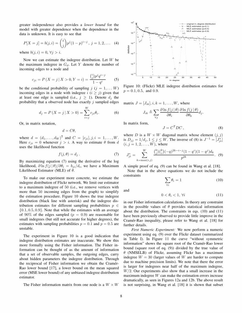
To make our experiment more concrete, we estimate the
indegree distribution of Flickr network. We limit our estimator
to a maximum indegree of 50 (i.e., we remove vertices with
more than 50 incoming edges from the graph) to simplify
the estimation procedure. Figure 10 shows the true indegree
distribution (black line with asterisk) and the indegree dis-
tribution estimates for different sampling probabilities p ∈{0.1, 0.5, 0.9}. Note that while the estimates with an average
of 90% of the edges sampled (p = 0.9) are reasonable for
small indegrees (but still not accurate for higher degrees), the
estimates with sampling probabilities p = 0.1 and p = 0.5 are
unstable.
The experiment in Figure 10 is a good indication that
indegree distribution estimates are inaccurate. We show this
more formally using the Fisher information. The Fisher in-
formation can be thought of as the amount of information
that a set of observable samples, the outgoing edges, carry
about hidden parameters the indegree distribution. Through
the reciprocal of Fisher information we obtain the Cramer-
Rao lower bound [17], a lower bound on the mean squared
error (MSE lower bound) of any unbiased indegree distribution
estimator.
The Fisher information matrix from one node is a W ×W
5 10 15 20 25 30 35 40 45 50
10−10
10−8
10−6
10−4
10−2
100
dist
ribut
ion
original in−degree distribution
MLE estimates (p=0.1)
MLE estimates (p=0.5)
MLE estimates (p=0.9)
in−degree
Figure 10: (Flickr) MLE indegree distribution estimates for
p = 0.1, 0.5, and 0.9.
matrix J = [Jik], i, k = 1, . . . ,W , where
Jik ,∑
∀j
∂ ln f(j | θ)∂θi
∂ ln f(j | θ)∂θk
dj .
In matrix form,
J = CTDC , (8)
where D is a W × W diagonal matrix whose element (j, j)is Djj = 1/dj, 1 ≤ j ≤ W . The inverse of (8) is J−1 = [J∗
ji](i, j = 1, 2, . . . ,W ), where
J∗ji =
W∑
k=max(i,j)
(
kj
)(
ki
)
(−q)2k−i−j(1− qi)(1− qj)dk
p2k. (9)
A simple proof of eq. (9) can be found in Wang et al. [18].
Note that in the above equations we do not include the
constraints∑
∀i
θi = 1 (10)
and
0 < θi < 1, ∀i (11)
in our Fisher information calculations. In theory any constraint
in the possible values of θ provides statistical information
about the distribution. The constraints in eqs. (10) and (11)
have been previously observed to provide little improve in the
Cramer-Rao inequality, please refer to Wang et al. [18] for
further details.
First Numeric Experiment: We now perform a numeric
experiment using eq. (9) over the Flickr dataset (summarized
in Table I). In Figure 11 the curve “without symmetric
information” shows the square root of the Cramer-Rao lower
bound (square root of eq. (9)) divided by the true value of
θ (NMSELB) of Flickr, assuming Flickr has a maximum
indegree W = 30 (larger values of W are harder to compute
due to machine precision limits). We note that there the error
is larger for indegrees near half of the maximum indegree,
W/2. Our experiments also show that a small increase in the
maximum indegreeW can make the estimation errors increase
dramatically, as seen in Figures 12a and 12b. The above result
is not surprising, in Wang et al. [18] it is shown that subset
8

0 5 10 15 20 25 3010
−4
10−2
100
102
104
106
108
1010
1012
in−degree
NM
SE
LB
without symmetric information (p=0.5)
without symmetric information (p=0.8)
with symmetric information (p=0.5)
with symmetric information (p=0.8)
Figure 11: (Flickr) Square root of the Cramer-Rao lower boundnormalized by the true value of θ. The curves show the error lowerbound with and without symmetric edge information. Edge symmetryat α = 62%. Lower is better.
size distribution estimation is impractical for large values of
W when sampling probabilities are less than (d−1)/(2d−1),where d is the average indegree.
The above experiment shows that we cannot accurately esti-
mate the indegree distribution of Flickr. The same experiment
with the remaining datasets of Table I achieves similar results.
There is hope, however. There are additional side information
available when estimating the indegree distribution that can
help reduce estimation errors. In what follows we consider
two side informations: average degree and edge symmetry,
where an edge u → v has a corresponding edge v → uwith probability p; some authors prefer to use the term edge
reciprocity.
0 5 10 15 20 25 3010
−4
10−2
100
102
104
106
108
in−degree
NM
SE
LB
W=5
W=30
(a) p = 0.5
0 5 10 15 20 25 3010
−4
10−3
10−2
10−1
100
101
102
103
in−degree
NM
SE
LB
W=5
W=30
(b) p = 0.8
Figure 12: (Flickr) The curves represent the error lower bound
when the maximum indegree W varies from 5 to 30, for
sampling rates p = 0.5 and p = 0.8, respectively.
Improving the Estimates with Side Information
There are additional side information available when esti-
mating the indegree distribution. For example, we know that
the average indegree is equal to the average outdegree. We
also know that some edges are symmetric (i.e., an incoming
edge has a corresponding outgoing edge).
A. Side information: Known average indegree
We have seen that DURW can provide good estimates
for the outdegree distribution and therefore for the average
outdegree. For the sake of argument, let’s even assume that
the average indegree µ is known. Knowing the indegree is
equivalent to adding the equality constraint
W∑
i=1
iθi = µ (12)
in the estimation problem. The statistical information given
by equation (12) can be added into the Fisher information as
follows. Let G = ∇θg(θ) be a column vector with the gradient
of g(θ) =∑W
i=1 iθi−µ in respect to θ1, . . . , θW . We now use
a result from Gorman and Hero [7] to include an equality
constraint in the Fisher information matrix and the Cramer-
Rao bound. The new Cramer-Rao bound accounting for the
increase in the Fisher information coming from the known the
average indegree is
J−1 − J−1GT(GJ−1GT)−1GJ−1, (13)
which is the old bound J−1 minus a term
J−1GT(GJ−1GT)−1GJ−1. Unfortunately, numerically,
eq. (13) is not significantly different from the original
Cramer-Rao bound, J−1. Thus, we rule out the average
indegree as relevant information to estimate the indegree
distribution.
A more promising property of many directed graphs is the
presence of symmetric edges. For example, in the Web-Google
dataset 69% of the edges are symmetric (the symmetry of
other datasets is in Table I). In a graph where all edges are
symmetric (i.e., every edge (u, v) ∈ Ed has a corresponding
edge (v, u) ∈ Ed) the indegree and the outdegree distributions
are the same. In what follows we consider a model that
adds such symmetric edge information to the estimation and
show that while moderate edge symmetry increases estimation
accuracy, it is still insufficient to obtain accurate estimates.
B. Side Information: Edge Symmetry
Consider a directed graph Gd = (V,Ed). Let s denote
the fraction of symmetric edges in Ed, where s = 1 when
all edges in Gd are symmetric. Edge symmetry can convey
information about the indegree distribution. For instance, if
s = 1 the indegree distribution is equivalent to the outdegree
distribution. To assess the increase in estimation accuracy that
comes from the presence of symmetric edges, consider the
following model.
Let v be a sampled vertex. Consider the following random
variables of v:
• Z: indegree of v.
• Zs: number of symmetric incoming edges.
• Za: number of incoming asymmetric edges.
• Y : observed outdegree.
• Xs observed number of symmetric incoming edges.
• Xa observed number of asymmetric incoming edges.
Also, let ρ(y, z) = P [Y = y, Z = z] be the joint indegree andoutdegree distribution of v, p be the sampling rate, and α be
the fraction of symmetric edges. We assume that the number of
outgoing edges of v that are symmetric is a Binomial random
9

variable with parameter α and has distribution
P [Zs = zs|Y = y, Z = z] ={
(
min(y,z)zs
)
αzs(1 − α)min(y,z)−zs if zs ≤ min(y, z),
0 otherwise.
(14)
We seek to find a likelihood function of the observed random
variables Y , Xs, and Xa with respect to ρ, P [Y = y,Xs =xs, Xa = xa|ρ]. Note that
P [Y = y,Xs = xs, Xa = xa|ρ]=
∑
∀z
P [Xs = xs, Xa = xa|Y = y, Z = z]ρy,z
=∑
∀z
ρy,z
z∑
zs=0
P [Xs = xs, Xa = xa|Zs = zs, Y = y, Z = z]
× P [Zs = zs|Y = y, Z = z],
where
P [Xs = xs, Xa = xa|Zs = zs, Y = y, Z = z]
= P [Xs = xs, Xa = xa|Zs = zs, Y = y, Za = z − zs]
=
(
zsxs
)
pxs(1− p)zs−xs
(
z − zsxa
)
pxa(1− p)z−zs−xa
=
(
zsxs
)(
z − zsxa
)
pxs+xa(1 − p)z−xs−xa
with P [Zs = zs|Y = y, Z = z] as defined in equation (14).
The indegree distribution Fisher information associated with
the symmetric edge information can be computed from the
Fisher information of P [Y = y,Xs = xs, Xa = xa|ρ] withrespect to ρ by noting that θ, the indegree distribution, can be
defined as θz =∑
∀y ρ(y, z) , ∀z, or in matrix form θ = HρT,where ρ = (ρ(1, 1), ρ(2, 1), . . . ) and
H =
1 . . . 1. . .
1 . . . 1
.
Let Jρ denote the Fisher information with respect to the joint
distribution ρ. Computing Jρ from P [Y = y,Xs = xs, Xa =xa|ρ] is trivial. Let Jθ denote the Fisher information with
respect to the indegree distribution θ. Then [17, pages 83–84]
Jθ = HJρHT.
Matrix Jθ encodes the information obtained from the observed
incoming edges plus the information that the graph is symmet-
ric. To obtain the Cramer-Rao bound we need to invert Jθ . We
do this inversion numerically in Section VI-C and observe that
adding symmetric information does not significantly improve
the estimation error unless most edges in the graph are
symmetric.
C. Numerical Results
In the following experiment we include symmetry informa-
tion in the Cramer-Rao lower bound computed by inverting Jθ(which is a bound on the mean squared error of any unbiased
estimator of θ). Figure 11 shows the square root of the Cramer-
Rao lower bound divided by the true value of θ (NMSELB)
of Flickr for maximum indegree W = 30, with and without
Flickr’s symmetric information. In Flickr the fraction of edges
that are symmetric is α = 0.62. Observe that while symmetry
reduces the Cramer-Rao lower bound, it is not enough to
significantly increases the estimation accuracy to acceptable
levels. Moreover, other experiments (not shown here) indicate
that increasing W significantly increases the estimation error
(to the point that even estimating θ1 can be made inaccurate).
VII. RELATED WORK
Estimating observable characteristics by sampling a directed
graph (in this case, the Web graph) has been the subject of
Bar-Yossef et al. [3] and Henzinger et al. [9], which transform
the directed graph of web-links into an undirected graph by
adding reverse links, and then use a Metropolis-Hastings RW
to sample webpages uniformly. Our “backward edge traversal”
is an adaptation of the method of Bar-Yossef et al. [3] to work
with a pure random walk and random jumps. Both of these
Metropolis-Hastings RWs are designed to sample directed
graph that do not allow random jumps. However, in the pres-
ence of random jumps (even if jumps are rare), the Metropolis-
Hastings RW algorithm is not as efficient and as accurate as
our DURW algorithm. Random walks with PageRank-style
jumps are used in Leskovec and Faloutsos [10] to sample large
graphs. In Leskovec and Faloutsos [10], however, there is no
technique to remove the large biases induced by the random
walk and the random jumps, which makes this method unfit
to estimate graph characteristics. In contrast, our distribution
estimates are asymptotically unbiased.
VIII. CONCLUSIONS & FUTURE WORK
In this work we provide the first random walk method to
accurately estimate characteristics of directed graphs that allow
random jumps. Also, to the best of our knowledge our work is
the first to study and provide a sound theoretical analysis of the
problem of estimating latent indegree distributions. Our future
work includes reducing the transient of our DURW algorithm.
REFERENCES
[1] Google Programming Contest. http://www.google.com/programming-contest/, 2002.
[2] Predicting Positive and Negative Links in Online Social Networks, 2010.[3] Ziv Bar-Yossef and Maxim Gurevich. Random sampling from a search
engine’s index. J. ACM, 55(5):1–74, 2008.[4] S. Brin and L. Page. The anatomy of a large-scale hypertextual Web
search engine. In Proc. of the WWW, 1998.[5] Facebook. http://www.facebook.com, 2010.[6] Flickr. http://www.flickr.com, July 2010.[7] John D. Gorman and Alfred O. Hero. Lower bounds for parametric
estimation with constraints. IEEE Transactions on Information Theory,36(6):1285–1301, Nov 1990.
[8] Douglas D. Heckathorn. Respondent-driven sampling: A new approachto the study of hidden populations. Social Problems, 1997.
[9] Monika R. Henzinger, Allan Heydon, Michael Mitzenmacher, and MarcNajork. On near-uniform url sampling. In Proceedings of the WWW,pages 295–308, 2000.
[10] Jure Leskovec and Christos Faloutsos. Sampling from large graphs. InProc. of the KDD, pages 631–636, 2006.
[11] Alan Mislove, Massimiliano Marcon, Krishna P. Gummadi, Peter Dr-uschel, and Bobby Bhattacharjee. Measurement and Analysis of OnlineSocial Networks. In Proc. of the IMC, October 2007.
[12] Amir H. Rasti, Mojtaba Torkjazi, Reza Rejaie, Nick Duffield, WalterWillinger, and Daniel Stutzbach. Respondent-driven sampling forcharacterizing unstructured overlays. In Proc. of the IEEE Infocom,pages 2701–2705, April 2009.
[13] Bruno Ribeiro, William Gauvin, Benyuan Liu, and Don Towsley. OnMySpace account spans and double Pareto-like distribution of friends.In Proceedings of the IEEE Infocom NetSciCom Workshop, 2010.
10

[14] Bruno Ribeiro and Don Towsley. Estimating and sampling graphs withmultidimensional random walks. In Proc. of the IMC, 2010.
[15] Bruno Ribeiro, Pinghui Wang, Fabricio Murai, and Don Towsley.Sampling directed graphs with random walks. Technical Report UM-CS-2011-031, UMass Amherst, 2011.
[16] D. Stutzbach, R. Rejaie, N. Duffield, S. Sen, and W. Willinger. Onunbiased sampling for unstructured peer-to-peer networks. IEEE/ACM
Trans. Netw., 17(2):377–390, 2009.[17] Hary L. van Trees. Estimation and Modulation Theory, Part 1. Wiley,
New York, 2001.[18] P. Wang, B. Ribeiro, and D. Towsley. On the cramer-rao bound of subset
size distribution estimation. Technical Report UM-CS-2011-029, UMassAmherst Computer Science, 2011.
[19] Wikipedia website. http://www.wikipedia.org, 2010.
11