Sample Size Calculations - MMB Home Page
223
Sample Size Calculations Practical Methods for Engineers and Scientists (Software solutions to selected example problems, Version: 17 August 2010)
Transcript of Sample Size Calculations - MMB Home Page

Sample Size CalculationsPractical Methods for Engineers and Scientists
(Software solutions to selected example problems, Version: 17 August 2010)


Sample Size CalculationsPractical Methods for Engineers and Scientists
(Software solutions to selected example problems, Version: 17 August 2010)
Paul Mathews

Sample Size Calculations: Practical Methods for Engineers and ScientistsPaul [email protected]
Copyright c 2010 Paul Mathews
All rights reserved. No part of this publication may be reproduced or stored in any form or by any means without the prior written permission of the publisher.
Published by:Mathews Malnar and Bailey, Inc.217 Third Street, Fairport Harbor, OH 44077Phone: 440-350-0911Fax: 440-350-7210Web: www.mmbstatistical.com
ISBN 978-0-615-32461-6
Original release: 24 February 2010

Contents
1 Fundamentals 71.1 Motivation for Sample Size Calculations . . . . . . . . . . . . . . . . . . . . . . . . . . . . . . . . . . . . . . . . . . . . . . . . . . . . . . . . . . . . . . . . . . . . . . . . 71.2 Rationale for Sample Size and Power Calculations . . . . . . . . . . . . . . . . . . . . . . . . . . . . . . . . . . . . . . . . . . . . . . . . . . . . . . . . . . . . . . . . . . 71.3 Rationale for Hypothesis Tests . . . . . . . . . . . . . . . . . . . . . . . . . . . . . . . . . . . . . . . . . . . . . . . . . . . . . . . . . . . . . . . . . . . . . . . . . . . . . . 121.4 Practical Considerations . . . . . . . . . . . . . . . . . . . . . . . . . . . . . . . . . . . . . . . . . . . . . . . . . . . . . . . . . . . . . . . . . . . . . . . . . . . . . . . . . 161.5 Problems and Solutions . . . . . . . . . . . . . . . . . . . . . . . . . . . . . . . . . . . . . . . . . . . . . . . . . . . . . . . . . . . . . . . . . . . . . . . . . . . . . . . . . 221.6 Software . . . . . . . . . . . . . . . . . . . . . . . . . . . . . . . . . . . . . . . . . . . . . . . . . . . . . . . . . . . . . . . . . . . . . . . . . . . . . . . . . . . . . . . . . . 22
2 Means 232.1 Assumptions . . . . . . . . . . . . . . . . . . . . . . . . . . . . . . . . . . . . . . . . . . . . . . . . . . . . . . . . . . . . . . . . . . . . . . . . . . . . . . . . . . . . . . . . 232.2 One Mean . . . . . . . . . . . . . . . . . . . . . . . . . . . . . . . . . . . . . . . . . . . . . . . . . . . . . . . . . . . . . . . . . . . . . . . . . . . . . . . . . . . . . . . . . 232.3 Two Independent Means . . . . . . . . . . . . . . . . . . . . . . . . . . . . . . . . . . . . . . . . . . . . . . . . . . . . . . . . . . . . . . . . . . . . . . . . . . . . . . . . . 352.4 Equivalence Tests . . . . . . . . . . . . . . . . . . . . . . . . . . . . . . . . . . . . . . . . . . . . . . . . . . . . . . . . . . . . . . . . . . . . . . . . . . . . . . . . . . . . . 472.5 Contrasts . . . . . . . . . . . . . . . . . . . . . . . . . . . . . . . . . . . . . . . . . . . . . . . . . . . . . . . . . . . . . . . . . . . . . . . . . . . . . . . . . . . . . . . . . . 512.6 Multiple Comparisons Tests . . . . . . . . . . . . . . . . . . . . . . . . . . . . . . . . . . . . . . . . . . . . . . . . . . . . . . . . . . . . . . . . . . . . . . . . . . . . . . . 52
3 Standard Deviations 573.1 One Standard Deviation . . . . . . . . . . . . . . . . . . . . . . . . . . . . . . . . . . . . . . . . . . . . . . . . . . . . . . . . . . . . . . . . . . . . . . . . . . . . . . . . . 573.2 Two Standard Deviations . . . . . . . . . . . . . . . . . . . . . . . . . . . . . . . . . . . . . . . . . . . . . . . . . . . . . . . . . . . . . . . . . . . . . . . . . . . . . . . . 633.3 Coefficient of Variation . . . . . . . . . . . . . . . . . . . . . . . . . . . . . . . . . . . . . . . . . . . . . . . . . . . . . . . . . . . . . . . . . . . . . . . . . . . . . . . . . . 68
4 Proportions 714.1 One Proportion (Large Population) . . . . . . . . . . . . . . . . . . . . . . . . . . . . . . . . . . . . . . . . . . . . . . . . . . . . . . . . . . . . . . . . . . . . . . . . . . . 714.2 One Proportion (Small Population) . . . . . . . . . . . . . . . . . . . . . . . . . . . . . . . . . . . . . . . . . . . . . . . . . . . . . . . . . . . . . . . . . . . . . . . . . . . 854.3 Two Proportions . . . . . . . . . . . . . . . . . . . . . . . . . . . . . . . . . . . . . . . . . . . . . . . . . . . . . . . . . . . . . . . . . . . . . . . . . . . . . . . . . . . . . . 884.4 Equivalence Tests . . . . . . . . . . . . . . . . . . . . . . . . . . . . . . . . . . . . . . . . . . . . . . . . . . . . . . . . . . . . . . . . . . . . . . . . . . . . . . . . . . . . . 984.5 Chi-square Tests . . . . . . . . . . . . . . . . . . . . . . . . . . . . . . . . . . . . . . . . . . . . . . . . . . . . . . . . . . . . . . . . . . . . . . . . . . . . . . . . . . . . . . 102
v

vi CONTENTS
5 Poisson Counts 1075.1 One Poisson Count . . . . . . . . . . . . . . . . . . . . . . . . . . . . . . . . . . . . . . . . . . . . . . . . . . . . . . . . . . . . . . . . . . . . . . . . . . . . . . . . . . . . 1075.2 Two Poisson Counts . . . . . . . . . . . . . . . . . . . . . . . . . . . . . . . . . . . . . . . . . . . . . . . . . . . . . . . . . . . . . . . . . . . . . . . . . . . . . . . . . . . 1155.3 Tests for Many Poisson Counts . . . . . . . . . . . . . . . . . . . . . . . . . . . . . . . . . . . . . . . . . . . . . . . . . . . . . . . . . . . . . . . . . . . . . . . . . . . . . 1195.4 Correcting for Background Counts . . . . . . . . . . . . . . . . . . . . . . . . . . . . . . . . . . . . . . . . . . . . . . . . . . . . . . . . . . . . . . . . . . . . . . . . . . . 120
6 Regression 1216.1 Linear Regression . . . . . . . . . . . . . . . . . . . . . . . . . . . . . . . . . . . . . . . . . . . . . . . . . . . . . . . . . . . . . . . . . . . . . . . . . . . . . . . . . . . . . 1216.2 Logistic Regression . . . . . . . . . . . . . . . . . . . . . . . . . . . . . . . . . . . . . . . . . . . . . . . . . . . . . . . . . . . . . . . . . . . . . . . . . . . . . . . . . . . . 128
7 Correlation and Agreement 1317.1 Pearson’s Correlation . . . . . . . . . . . . . . . . . . . . . . . . . . . . . . . . . . . . . . . . . . . . . . . . . . . . . . . . . . . . . . . . . . . . . . . . . . . . . . . . . . . 1317.2 Intraclass Correlation . . . . . . . . . . . . . . . . . . . . . . . . . . . . . . . . . . . . . . . . . . . . . . . . . . . . . . . . . . . . . . . . . . . . . . . . . . . . . . . . . . . 1357.3 Cohen’s Kappa . . . . . . . . . . . . . . . . . . . . . . . . . . . . . . . . . . . . . . . . . . . . . . . . . . . . . . . . . . . . . . . . . . . . . . . . . . . . . . . . . . . . . . 1377.4 Receiver Operating Characteristic (ROC) Curves . . . . . . . . . . . . . . . . . . . . . . . . . . . . . . . . . . . . . . . . . . . . . . . . . . . . . . . . . . . . . . . . . . . 1397.5 Bland-Altman Plots . . . . . . . . . . . . . . . . . . . . . . . . . . . . . . . . . . . . . . . . . . . . . . . . . . . . . . . . . . . . . . . . . . . . . . . . . . . . . . . . . . . . 142
8 Designed Experiments 1458.1 One-Way Fixed Effects ANOVA . . . . . . . . . . . . . . . . . . . . . . . . . . . . . . . . . . . . . . . . . . . . . . . . . . . . . . . . . . . . . . . . . . . . . . . . . . . . . 1458.2 Randomized Block Design . . . . . . . . . . . . . . . . . . . . . . . . . . . . . . . . . . . . . . . . . . . . . . . . . . . . . . . . . . . . . . . . . . . . . . . . . . . . . . . . 1528.3 Balanced Full Factorial Design with Fixed Effects . . . . . . . . . . . . . . . . . . . . . . . . . . . . . . . . . . . . . . . . . . . . . . . . . . . . . . . . . . . . . . . . . . . 1538.4 Random and Mixed Models . . . . . . . . . . . . . . . . . . . . . . . . . . . . . . . . . . . . . . . . . . . . . . . . . . . . . . . . . . . . . . . . . . . . . . . . . . . . . . . 1598.5 Nested Designs . . . . . . . . . . . . . . . . . . . . . . . . . . . . . . . . . . . . . . . . . . . . . . . . . . . . . . . . . . . . . . . . . . . . . . . . . . . . . . . . . . . . . . 1618.6 Two-Level Factorial Designs . . . . . . . . . . . . . . . . . . . . . . . . . . . . . . . . . . . . . . . . . . . . . . . . . . . . . . . . . . . . . . . . . . . . . . . . . . . . . . . 1628.7 Two-Level Factorial Designs with Centers . . . . . . . . . . . . . . . . . . . . . . . . . . . . . . . . . . . . . . . . . . . . . . . . . . . . . . . . . . . . . . . . . . . . . . . 1718.8 Response Surface Designs . . . . . . . . . . . . . . . . . . . . . . . . . . . . . . . . . . . . . . . . . . . . . . . . . . . . . . . . . . . . . . . . . . . . . . . . . . . . . . . . 172
9 Reliability and Survival 1759.1 Reliability Parameter Estimation . . . . . . . . . . . . . . . . . . . . . . . . . . . . . . . . . . . . . . . . . . . . . . . . . . . . . . . . . . . . . . . . . . . . . . . . . . . . 1759.2 Reliability Demonstration Tests . . . . . . . . . . . . . . . . . . . . . . . . . . . . . . . . . . . . . . . . . . . . . . . . . . . . . . . . . . . . . . . . . . . . . . . . . . . . . 1819.3 Two-Sample Reliability Tests . . . . . . . . . . . . . . . . . . . . . . . . . . . . . . . . . . . . . . . . . . . . . . . . . . . . . . . . . . . . . . . . . . . . . . . . . . . . . . 1899.4 Interference . . . . . . . . . . . . . . . . . . . . . . . . . . . . . . . . . . . . . . . . . . . . . . . . . . . . . . . . . . . . . . . . . . . . . . . . . . . . . . . . . . . . . . . . 192
10 Statistical Quality Control 19510.1 Statistical Process Control . . . . . . . . . . . . . . . . . . . . . . . . . . . . . . . . . . . . . . . . . . . . . . . . . . . . . . . . . . . . . . . . . . . . . . . . . . . . . . . . 19510.2 Process Capability . . . . . . . . . . . . . . . . . . . . . . . . . . . . . . . . . . . . . . . . . . . . . . . . . . . . . . . . . . . . . . . . . . . . . . . . . . . . . . . . . . . . . 19710.3 Tolerance Intervals . . . . . . . . . . . . . . . . . . . . . . . . . . . . . . . . . . . . . . . . . . . . . . . . . . . . . . . . . . . . . . . . . . . . . . . . . . . . . . . . . . . . 19910.4 Acceptance Sampling . . . . . . . . . . . . . . . . . . . . . . . . . . . . . . . . . . . . . . . . . . . . . . . . . . . . . . . . . . . . . . . . . . . . . . . . . . . . . . . . . . . 20010.5 Gage R&R Studies . . . . . . . . . . . . . . . . . . . . . . . . . . . . . . . . . . . . . . . . . . . . . . . . . . . . . . . . . . . . . . . . . . . . . . . . . . . . . . . . . . . . . 211

CONTENTS vii
11 Resampling Methods 21311.1 Software Requirements . . . . . . . . . . . . . . . . . . . . . . . . . . . . . . . . . . . . . . . . . . . . . . . . . . . . . . . . . . . . . . . . . . . . . . . . . . . . . . . . . . 21311.2 Monte Carlo . . . . . . . . . . . . . . . . . . . . . . . . . . . . . . . . . . . . . . . . . . . . . . . . . . . . . . . . . . . . . . . . . . . . . . . . . . . . . . . . . . . . . . . . 21311.3 Bootstrap . . . . . . . . . . . . . . . . . . . . . . . . . . . . . . . . . . . . . . . . . . . . . . . . . . . . . . . . . . . . . . . . . . . . . . . . . . . . . . . . . . . . . . . . . . 214

viii CONTENTS

CONTENTS 1
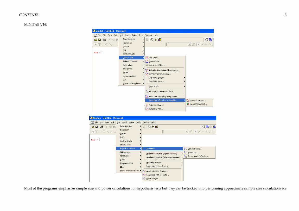
The purpose of this document is to present solutions to selected example problems from the book using PASS (2005), MINITAB (V15 and V16), Piface (V1.72), and R. (Thisversion of the document, compiled on 17 August 2010, does not yet contain solutions using R.) All of the programs have more sample size and power calculation capabilitiesthan what is included in the book. Some packages are particularly strong in certain areas. For example, PASS has the broadest scope, Piface offers an unmatched collection ofANOVA methods involving fixed, random, mixed, and nested designs and supports custom ANOVA models, and MINITAB has special methods for quality engineers includingattribute and variables sampling plan design and reliability study design.
The following figures show screen captures of some of the methods available in Piface, PASS, and MINITAB.

2 CONTENTS
MINITAB V15:
CONTENTS 3
MINITAB V16:
Most of the programs emphasize sample size and power calculations for hypothesis tests but they can be tricked into performing approximate sample size calculations for

4 CONTENTS

CONTENTS 5
confidence intervals by setting the hypothesis test power to � = 0:50. This trick is exact when the sampling distribution is normal because z0:50 = 0 and it is reasonably accuratewhen the sampling distribution is other than normal but symmetric. Be more careful when the sampling distribution is asymmetric.
The solutions in the book don’t use the continuity correction when discrete distributions are approximated with continuous ones, however, the software solutions ofteninclude the continuity correction so answers to problems may differ slightly. If you have access to software that provides more accurate methods, then definitely use thesoftware.
Some software provides several analysis methods for the same problem. For example, PASS offers six different methods for the significance test for one proportion expressedin terms of the proportion difference. The different methods usually give similar answers.
This document will be revised occasionally. The current version was compiled on 17 August 2010.

6 CONTENTS

Chapter 1
Fundamentals
1.1 Motivation for Sample Size Calculations
1.2 Rationale for Sample Size and Power Calculations
Example 1.1 Express the confidence interval P (3:1 < � < 3:7) = 0:95 in words.Solution: The confidence interval indicates that we can be 95% confident that the true but unknown value of the population mean � falls between � = 3:1 and � = 3:7.Apparently, the mean of the sample used to construct the confidence interval is �x = 3:4 and the confidence interval half-width is � = 0:3.
Example 1.2 Data are to be collected for the purpose of estimating the mean of a mechanical measurement. Data from a similar process suggest that the standard deviation willbe �x = 0:003mm. Determine the sample size required to estimate the value of the population mean with a 95% confidence interval of half-width � = 0:002mm.Solution: With z�=2 = z0:025 = 1:96 in Equation 1.4, the required sample size is
n =
�1:96� 0:0030:002
�2= 8:64.
The sample size must be an integer; therefore, we round the calculated value of n up to n = 9.
From MINITAB> Stat> Power and Sample Size> 1-Sample Z:
7
8 Chapter 1. Fundamentals
From PASS>Means>One> Confidence Interval of Mean:
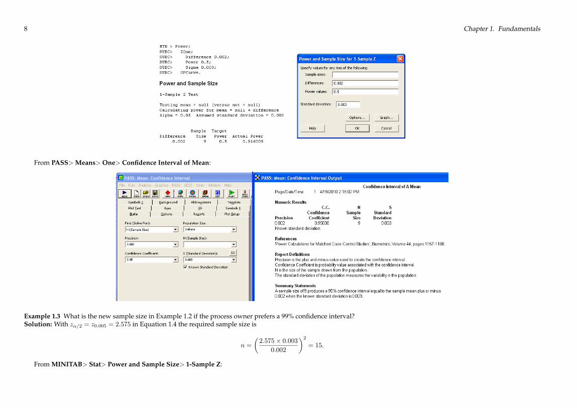
Example 1.3 What is the new sample size in Example 1.2 if the process owner prefers a 99% confidence interval?Solution: With z�=2 = z0:005 = 2:575 in Equation 1.4 the required sample size is
n =
�2:575� 0:003
0:002
�2= 15.
From MINITAB> Stat> Power and Sample Size> 1-Sample Z:

1.2. Rationale for Sample Size and Power Calculations 9
From PASS>Means>One> Confidence Interval of Mean:
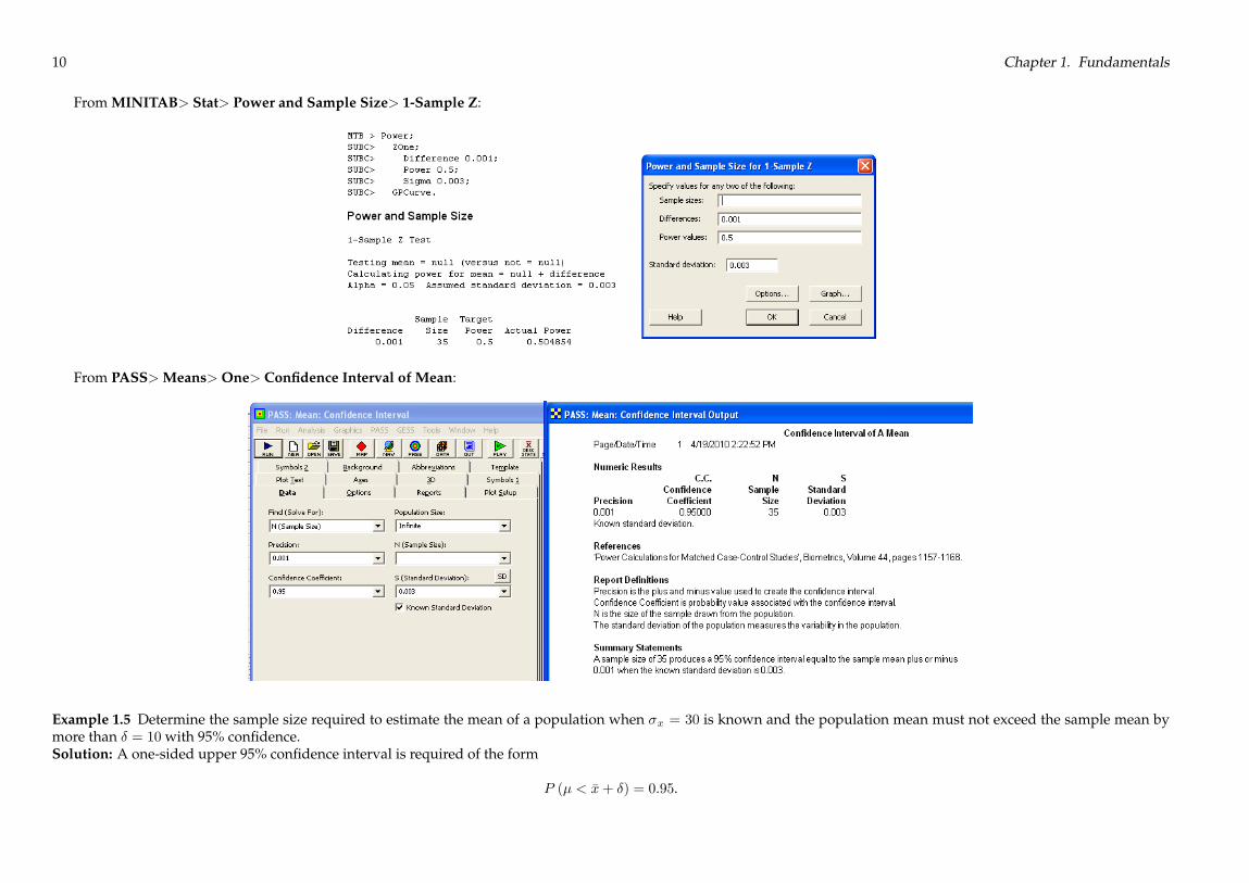
Example 1.4 What is the new sample size in Example 1.2 if the process owner prefers a 95% confidence level with � = 0:001mm half-width?Solution: With z0:025 = 1:96 and � = 0:001mm in Equation 1.4 the required sample size is
n =
�1:96� 0:0030:001
�2= 35.
10 Chapter 1. Fundamentals
From MINITAB> Stat> Power and Sample Size> 1-Sample Z:
From PASS>Means>One> Confidence Interval of Mean:
Example 1.5 Determine the sample size required to estimate the mean of a population when �x = 30 is known and the population mean must not exceed the sample mean bymore than � = 10with 95% confidence.Solution: A one-sided upper 95% confidence interval is required of the form
P (� < �x+ �) = 0:95.
1.2. Rationale for Sample Size and Power Calculations 11
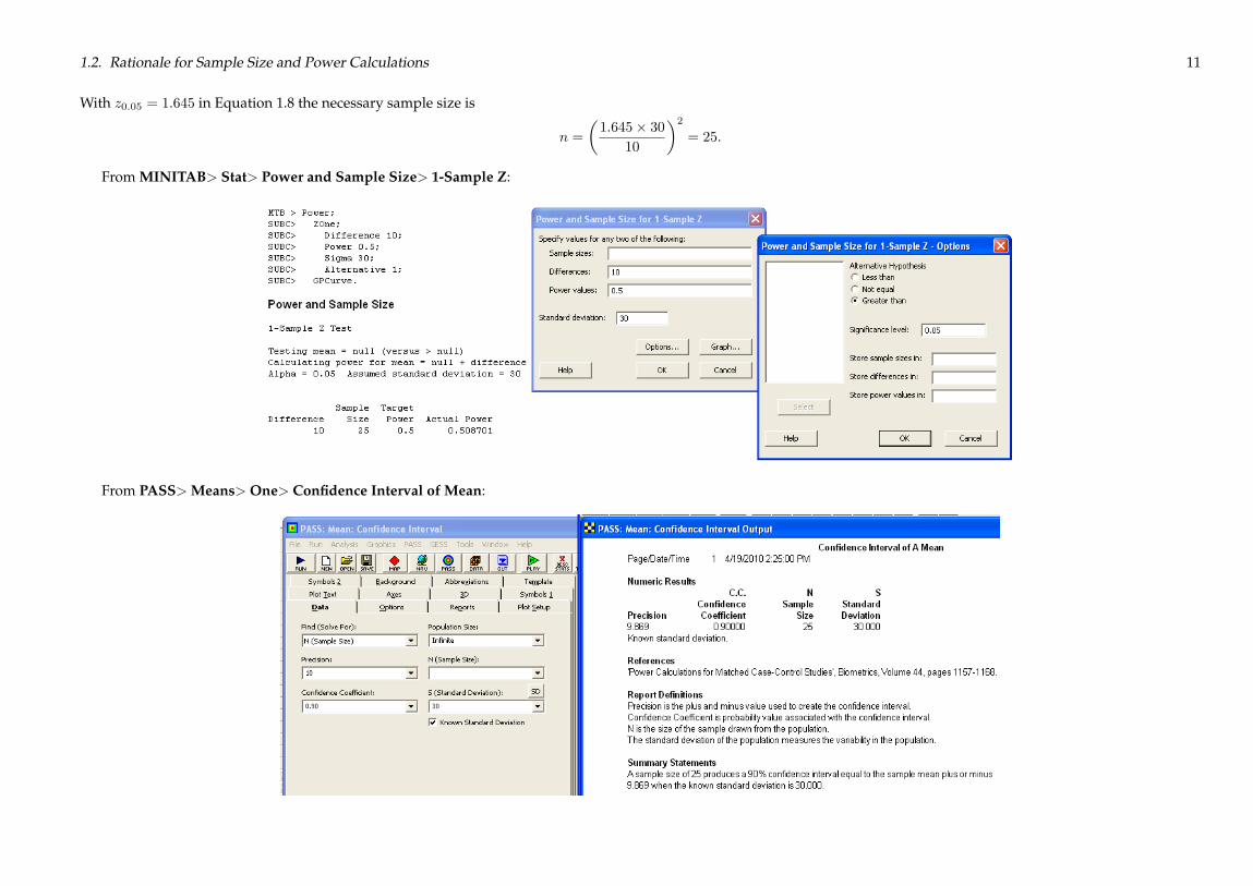
With z0:05 = 1:645 in Equation 1.8 the necessary sample size is
n =
�1:645� 30
10
�2= 25:
From MINITAB> Stat> Power and Sample Size> 1-Sample Z:
From PASS>Means>One> Confidence Interval of Mean:
12 Chapter 1. Fundamentals
1.3 Rationale for Hypothesis Tests
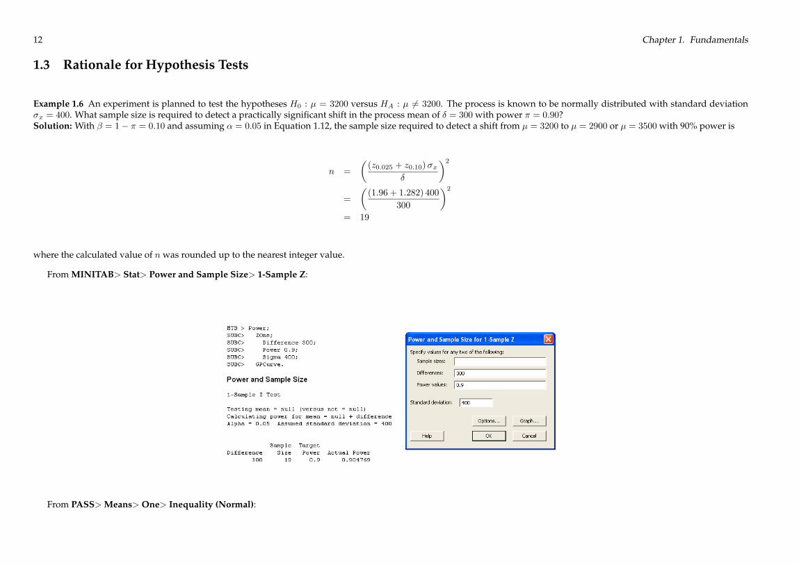
Example 1.6 An experiment is planned to test the hypotheses H0 : � = 3200 versus HA : � 6= 3200. The process is known to be normally distributed with standard deviation�x = 400. What sample size is required to detect a practically significant shift in the process mean of � = 300 with power � = 0:90?Solution: With � = 1� � = 0:10 and assuming � = 0:05 in Equation 1.12, the sample size required to detect a shift from � = 3200 to � = 2900 or � = 3500 with 90% power is
n =
�(z0:025 + z0:10)�x
�
�2=
�(1:96 + 1:282) 400
300
�2= 19
where the calculated value of n was rounded up to the nearest integer value.
From MINITAB> Stat> Power and Sample Size> 1-Sample Z:
From PASS>Means>One> Inequality (Normal):

1.3. Rationale for Hypothesis Tests 13
Example 1.7 An experiment will be performed to test H0 : � = 8:0 versus HA : � > 8:0. What sample size is required to reject H0 with 90% power when � = 8:2? The process isknown to be normally distributed with �x = 0:2.Solution: For the one-tailed hypothesis test with � = 0:05, � = 0:2 and � = 1� � = 0:10 the required sample size is
n =
�(z� + z�)�x
�
�2=
�(z0:05 + z10)�x
�
�2=
�(1:645 + 1:282) 0:2
0:2
�2= 9.
From MINITAB> Stat> Power and Sample Size> 1-Sample Z:

14 Chapter 1. Fundamentals
From PASS>Means>One> Inequality (Normal):
Example 1.8 Calculate the p value for the test performed under the conditions of Example 1.6 if the sample mean was �x = 3080.

1.3. Rationale for Hypothesis Tests 15
Solution: Figure 1.4 shows the contributions to the p value from the two tails of the �x distribution under H0. The z test statistic that corresponds to �x is
z =�x� �0��x
=�x� �0�x=
pn
=3080� 3200400=
p19
= �1:31,
so the p value is
p = 1� � (�1:31 < z < 1:31)= 0:19.
Because (p = 0:19) > (� = 0:05), the observed sample mean is statistically consistent with H0 : � = 3200, so we can not reject H0.From MINITAB> Stat> Power and Sample Size> 1-Sample Z:
Example 1.9 Calculate the p value for the test performed under the conditions of Example 1.7 if the sample mean was �x = 8:39.Solution: Figure 1.5 shows the single contribution to the p value from the right tail of the �x distribution under H0. The z test statistic that corresponds to �x is
z =8:39� 8:20:2=
p9
= 2:85,

16 Chapter 1. Fundamentals
so the p value is
p = �(2:85 < z <1)= 0:0022.
Because (p = 0:0022) < (� = 0:05), the observed sample mean is an improbable result under H0 : � = 8:2, so we must reject H0.From MINITAB> Stat> Power and Sample Size> 1-Sample Z:
1.4 Practical Considerations
Example 1.10 What sample size is required for a pilot study to estimate the standard deviation to be used in the sample size calculation for a primary experiment if the samplesize for the primary experiment should be within 20% of the correct value with 90% confidence?Solution: With � = 0:20 and � = 0:10 in Equation 1.20, the required sample size for the preliminary experiment to estimate the standard deviation is
n ' 2
�1:645
0:20
�2' 136.
From Piface> Pilot Study:
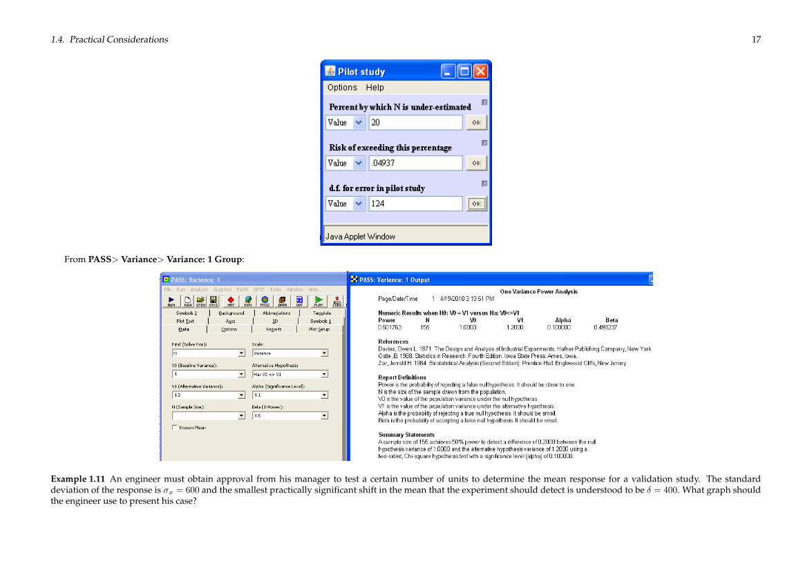
1.4. Practical Considerations 17
From PASS> Variance> Variance: 1 Group:
Example 1.11 An engineer must obtain approval from his manager to test a certain number of units to determine the mean response for a validation study. The standarddeviation of the response is �x = 600 and the smallest practically significant shift in the mean that the experiment should detect is understood to be � = 400. What graph shouldthe engineer use to present his case?

18 Chapter 1. Fundamentals
Solution: The value of the effect size of interest is firm at � = 400. The sample size is going to affect the power of the test, so an appropriate graph is power versus sample size.The sample size required to obtain a specified value of power for the test of H0 : � = 0 versus HA : � 6= 0 is given by Equation 1.12. Figure 1.6 shows the resulting power curve.The sample size required to obtain 80% power is n = 18 and the sample size required for 90% power is n = 24.
From MINITAB> Stat> Power and Sample Size> 1-Sample Z:
From PASS>Means>One> Inequality (Normal):

1.4. Practical Considerations 19

20 Chapter 1. Fundamentals
Example 1.12 Suppose that the manager in Example 1.11 approves the use of n = 24 units in the validation study. What power does the study have to reject H0 when the effectsize is � = 200, 400, and 600?7
Solution: The power is given by
� = �(�z� < z <1)
where z� is determined from Equation 1.12:
z� =pn�
�x� z�=2.
Figure 1.7 shows the power as a function of effect size. The power to reject H0 when � = 200 is � ' 0:37, when � = 400 is � ' 0:90, and when � = 600 is � ' 1.
From MINITAB> Stat> Power and Sample Size> 1-Sample Z:

1.4. Practical Considerations 21
From PASS>Means>One> Inequality (Normal):

22 Chapter 1. Fundamentals
1.5 Problems and Solutions
1.6 Software
Chapter 2
Means
2.1 Assumptions
2.2 One Mean
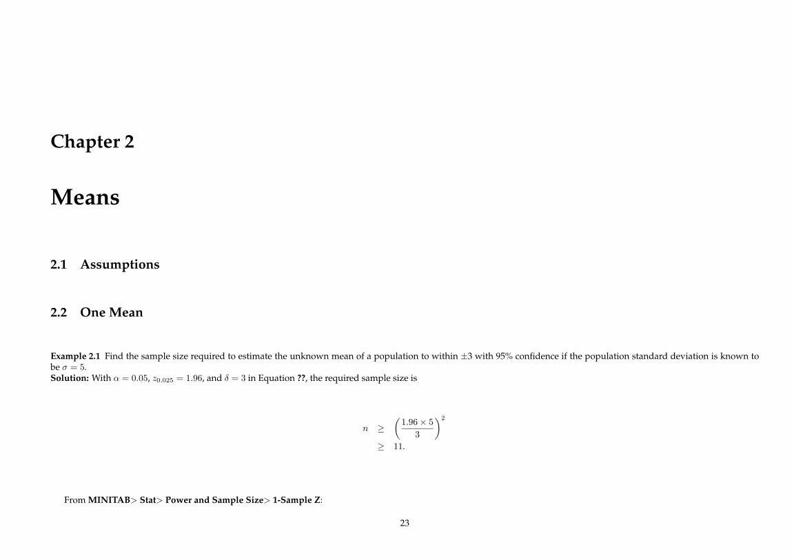
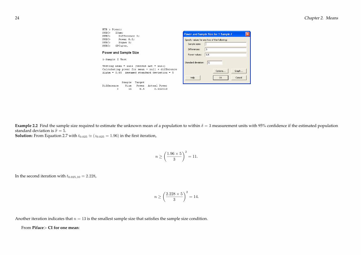
Example 2.1 Find the sample size required to estimate the unknown mean of a population to within �3 with 95% confidence if the population standard deviation is known tobe � = 5.Solution: With � = 0:05, z0:025 = 1:96, and � = 3 in Equation ??, the required sample size is
n ��1:96� 53
�2� 11.
From MINITAB> Stat> Power and Sample Size> 1-Sample Z:
23
24 Chapter 2. Means
Example 2.2 Find the sample size required to estimate the unknown mean of a population to within � = 3 measurement units with 95% confidence if the estimated populationstandard deviation is b� = 5.Solution: From Equation 2.7 with t0:025 ' (z0:025 = 1:96) in the first iteration,
n ��1:96� 53
�2= 11.
In the second iteration with t0:025;10 = 2:228,
n ��2:228� 5
3
�2= 14.
Another iteration indicates that n = 13 is the smallest sample size that satisfies the sample size condition.
From Piface> CI for one mean:

2.2. One Mean 25
From MINITAB> Stat> Power and Sample Size> 1-Sample t:
From MINITAB (V16)> Stat> Power and Sample Size> Sample Size for Estimation>Mean (Normal):

26 Chapter 2. Means
From PASS>Means>One> Confidence Interval of Mean:
Example 2.3 For the one-sample test of H0 : � = 30 versus HA : � 6= 30 when the population is known to be normal with � = 3, what sample size is required to detect a shift to� = 32with 90% power?Solution: By Equation 2.16 with � = 2, z0:025 = 1:96, and z0:10 = 1:28, the necessary sample size is
n � (1:96 + 1:28)2�3
2
�2= 24.

2.2. One Mean 27
From PASS>Means>One> Inequality (Normal):
Example 2.4 For the one-sample test of H0 : � = 30 versus HA : � 6= 30, what sample size is required to detect a shift to � = 32 with 90% power? The population standarddeviation is unknown but expected to be � ' 1:5.Solution: The sample size condition given by Equation 2.21 is transcendental, so the correct value of n must be determined iteratively. With t ' z as a first guess, z0:025 = 1:96,z0:10 = 1:282, and
n = (1:96 + 1:282)2
�1:5
2
�2= 6.
Then with df� = 5, t0:025;5 = 2:571, and t0:10;5 = 1:476 the new sample size estimate is
n � (2:571 + 1:476)2�1:5
2
�2= 9:21.
Further iterations are required because (n = 6) � 9:21. Another iteration indicates that n = 9 delivers the desired power.From Piface>One-sample t test (or paired t):

28 Chapter 2. Means
From MINITAB> Stat> Power and Sample Size> 1-Sample t:

2.2. One Mean 29
From PASS>Means>One> Inequality (Normal):
Example 2.5 Find the approximate and exact power for the solution obtained for Example 2.4.Solution: With n = 9 and t0:025;8 = 2:306 the approximate power by Equation 2.19 is
� = P
��1 < t <
�b�=pn � t�=2�
= P
��1 < t <
2
1:5=p9� 2:306
�= P (�1 < t < 1:694)
= 0:9356.
From Equation 2.23 the t distribution noncentrality parameter is
� =2
1:5=p9= 4:00,
so, from Equation 2.22,t0:025 = 2:306 = t�;4:0,

30 Chapter 2. Means
which is satisfied by � = 0:0633 and power � = 1�� = 0:9367. This value is in excellent agreement with the value obtained by the approximate method even though the samplesize is relatively small.
From Piface>One-sample t test (or paired t):
Example 2.6 Compare the sample sizes for the two-independent-samples experiment and the paired-sample experiment if they must detect a bias between two treatments of�� = 2 with 90% power when the standard deviation of individual units is b�x = 2 and the measurement precision error is b�� = 0:5.Solution: For the two-independent-sample t test the characteristic standard deviation for each treatment is (from Equation 2.27)
b�independent =p22 + 0:52 = 2:062.
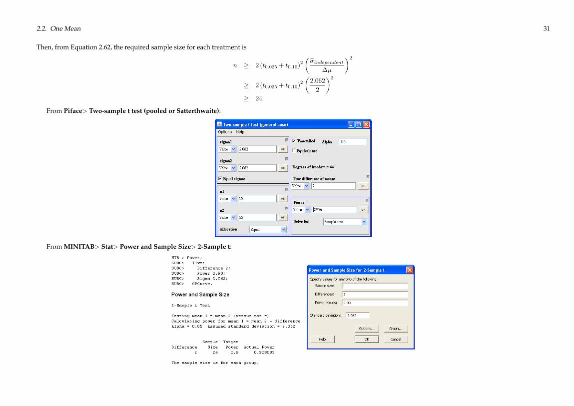
2.2. One Mean 31
Then, from Equation 2.62, the required sample size for each treatment is
n � 2 (t0:025 + t0:10)2
�b�independent��
�2� 2 (t0:025 + t0:10)
2
�2:062
2
�2� 24.
From Piface> Two-sample t test (pooled or Satterthwaite):
From MINITAB> Stat> Power and Sample Size> 2-Sample t:

32 Chapter 2. Means
From PASS>Means> Two> Independent> Inequality (Normal) [Differences]:
For the paired-sample t test, the characteristic standard deviation for the �xi can be estimated from Equation 2.28:
b��x = p2b�� = p2� 0:5 = 0:707.Then, from Equation 2.21, the required sample size is approximately
n � (t0:025 + t0:10)2
�b��x��
�2� (t0:025 + t0:10)
2
�0:707
2
�2� 4
and further iterations confirm that n = 4. When the independent-samples design requires two samples of size n = 24 units each, for a total of 48measurements, the paired-sampledesign requires only n = 4 units for a total of 8measurements!
From Piface>One-sample t test (or paired t):

2.2. One Mean 33
From MINITAB (V16)> Stat> Power and Sample Size> Paired t:
From MINITAB> Stat> Power and Sample Size> 1-Sample t:

34 Chapter 2. Means
From PASS>Means>One> Inequality (Normal):
2.3. Two Independent Means 35
2.3 Two Independent Means
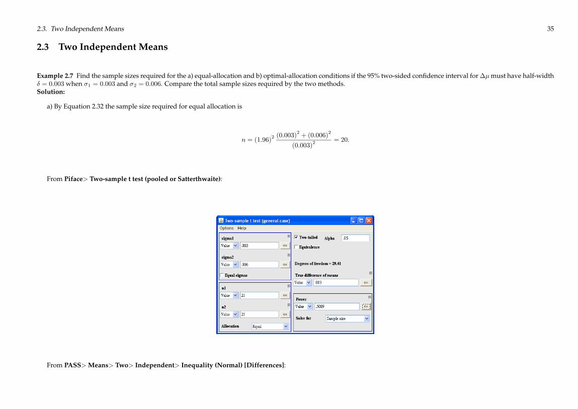
Example 2.7 Find the sample sizes required for the a) equal-allocation and b) optimal-allocation conditions if the 95% two-sided confidence interval for��must have half-width� = 0:003when �1 = 0:003 and �2 = 0:006. Compare the total sample sizes required by the two methods.Solution:
a) By Equation 2.32 the sample size required for equal allocation is
n = (1:96)2 (0:003)
2+ (0:006)
2
(0:003)2 = 20.
From Piface> Two-sample t test (pooled or Satterthwaite):
From PASS>Means> Two> Independent> Inequality (Normal) [Differences]:
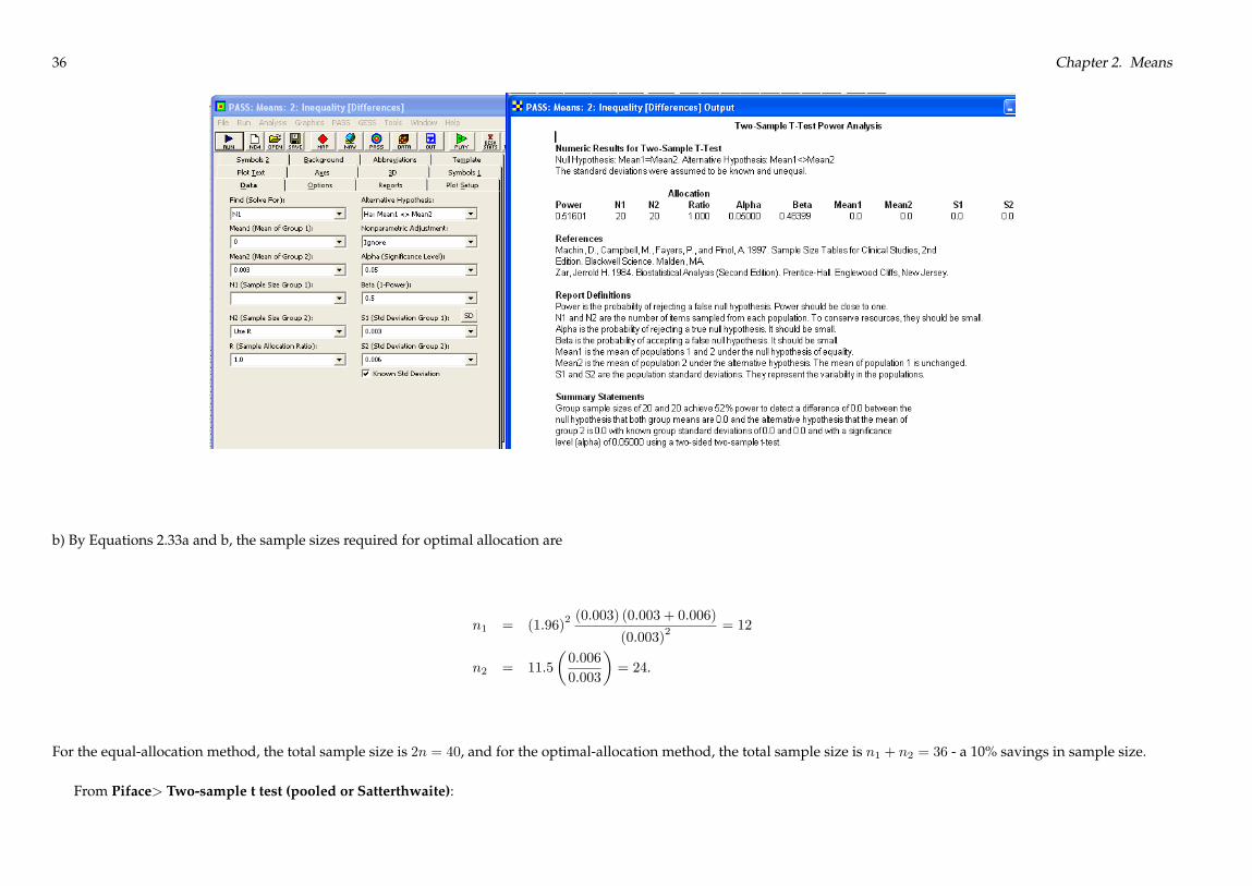
36 Chapter 2. Means
b) By Equations 2.33a and b, the sample sizes required for optimal allocation are
n1 = (1:96)2 (0:003) (0:003 + 0:006)
(0:003)2 = 12
n2 = 11:5
�0:006
0:003
�= 24.
For the equal-allocation method, the total sample size is 2n = 40, and for the optimal-allocation method, the total sample size is n1 + n2 = 36 - a 10% savings in sample size.
From Piface> Two-sample t test (pooled or Satterthwaite):

2.3. Two Independent Means 37
Example 2.8 Determine the sample size required to obtain a confidence interval half-width � = 50 when b�1 = b�2 = 80.Solution: With t0:025 ' z0:025 for the first iteration, the sample size is
n = 2
�1:96� 8050
�2= 20. (2.1)
Another iteration with t0:025;38 = 2:024 gives
n = 2
�2:024� 80
50
�2= 21. (2.2)
A third iteration (not shown) confirms that n = 21 is the necessary sample size.
From Piface> Two-sample t test (pooled or Satterthwaite):

38 Chapter 2. Means
From MINITAB> Stat> Power and Sample Size> 2-Sample t:
From PASS>Means> Two> Independent> Inequality (Normal) [Differences]:

2.3. Two Independent Means 39
Example 2.9 What optimal sample sizes are required to determine a confidence interval for the difference between two population means with confidence interval half-width� = 15when b�1 = 24 and b�2 = 8?
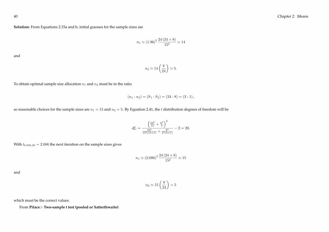
40 Chapter 2. Means
Solution: From Equations 2.33a and b, initial guesses for the sample sizes are
n1 ' (1:96)224 (24 + 8)
152' 14
and
n2 ' 14�8
24
�' 5.
To obtain optimal sample size allocation n1 and n2 must be in the ratio
(n1 : n2) = (b�1 : b�2) = (24 : 8) = (3 : 1) ,
so reasonable choices for the sample sizes are n1 = 15 and n2 = 5. By Equation 2.41, the t distribution degrees of freedom will be
df� =
�242
15 +82
5
�2244
152(15+1) +84
52(5+1)
� 2 = 20.
With t0:025;20 = 2:086 the next iteration on the sample sizes gives
n1 ' (2:086)224 (24 + 8)
152' 15
and
n2 ' 15�8
24
�= 5
which must be the correct values.
From Piface> Two-sample t test (pooled or Satterthwaite):

2.3. Two Independent Means 41
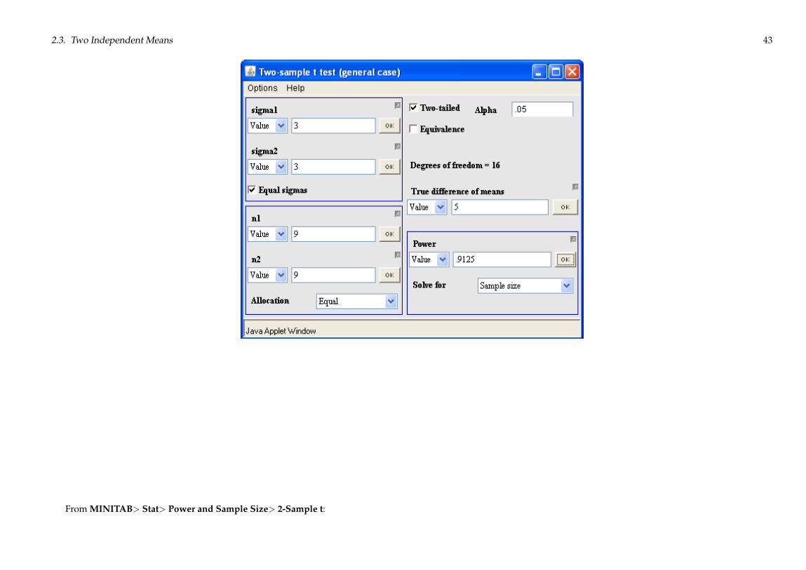
Example 2.10 Calculate the sample size for the two-sample t test to reject H0 with 90% power when j�1 � �2j = 5. Assume that the sample sizes will be equal and that the twopopulations have equal standard deviations estimated to be b�� = 3. Compare the approximate and exact powers.Solution: With �� = 5 and b�� = 3 in Equation 2.62, the sample size predicted in the first iteration with t ' z is
n = 2
�(1:96 + 1:282) 3
5
�2= 8.
A second and third iteration indicate that the required sample size is n = 9.
42 Chapter 2. Means
With n = 9 for both samples, df� = 18� 2 = 16 and the approximate power is given by Equations 2.58 and 2.60:
� = P
��1 < t <
rn
2
��b�� � t0:025;16�
= P
�1 < t <
r9
2
5
3� 2:12
!= P (�1 < t < 1:416)
= 0:912.
The t distribution noncentrality parameter is given by Equation 2.64:
� =
r9
2
5
3= 3:536.
The exact power is determined by Equation 2.63 with � = 0:05:
t0:025 = 2:120 = t�;3:536,
which is satisfied by � = 0:087, so the exact power is � = 0:913. The exact power is in excellent agreement with the approximate power despite the somewhat small sample size.
From Piface> Two-sample t test (pooled or Satterthwaite):
2.3. Two Independent Means 43
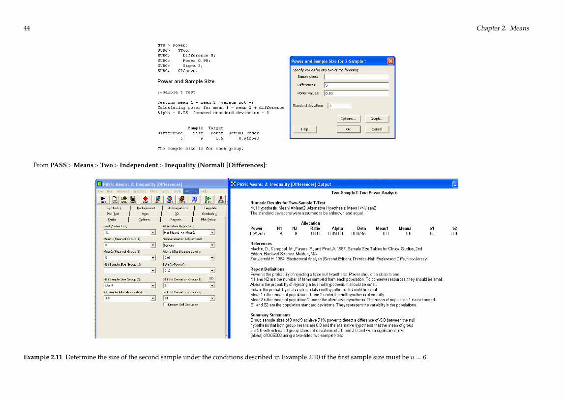
From MINITAB> Stat> Power and Sample Size> 2-Sample t:
44 Chapter 2. Means
From PASS>Means> Two> Independent> Inequality (Normal) [Differences]:
Example 2.11 Determine the size of the second sample under the conditions described in Example 2.10 if the first sample size must be n = 6.
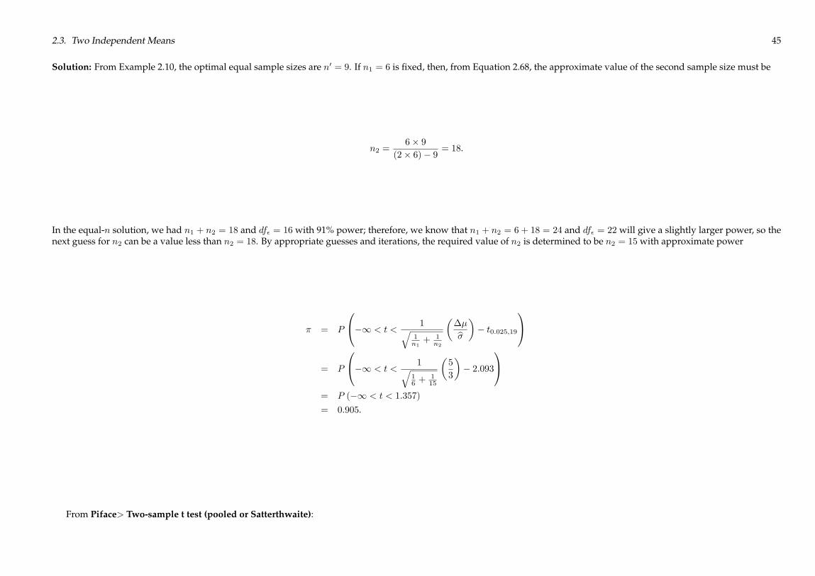
2.3. Two Independent Means 45
Solution: From Example 2.10, the optimal equal sample sizes are n0 = 9. If n1 = 6 is fixed, then, from Equation 2.68, the approximate value of the second sample size must be
n2 =6� 9
(2� 6)� 9 = 18.
In the equal-n solution, we had n1 + n2 = 18 and df� = 16 with 91% power; therefore, we know that n1 + n2 = 6 + 18 = 24 and df� = 22 will give a slightly larger power, so thenext guess for n2 can be a value less than n2 = 18. By appropriate guesses and iterations, the required value of n2 is determined to be n2 = 15 with approximate power
� = P
0@�1 < t <1q
1n1+ 1
n2
���b��� t0:025;19
1A= P
0@�1 < t <1q
16 +
115
�5
3
�� 2:093
1A= P (�1 < t < 1:357)
= 0:905.
From Piface> Two-sample t test (pooled or Satterthwaite):
46 Chapter 2. Means
From PASS>Means> Two> Independent> Inequality (Normal) [Differences]:

2.4. Equivalence Tests 47
2.4 Equivalence Tests
Example 2.12 Determine the sample size required for a one-sample equivalence test of the hypothesesH0 : � < 490 or � > 510 versusHA : 490 < � < 510 if the experiment musthave 90% power to reject H0 when � = 505 and � = 4.Solution: With �0 = 500, � = 505, and � = 10, the sample size given by Equation 2.74 is
n =
�(z0:05 + z0:10)�
� ���
�2=
�(1:645 + 1:282) 4
10� 5
�2= 6.
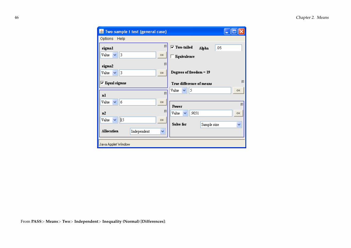
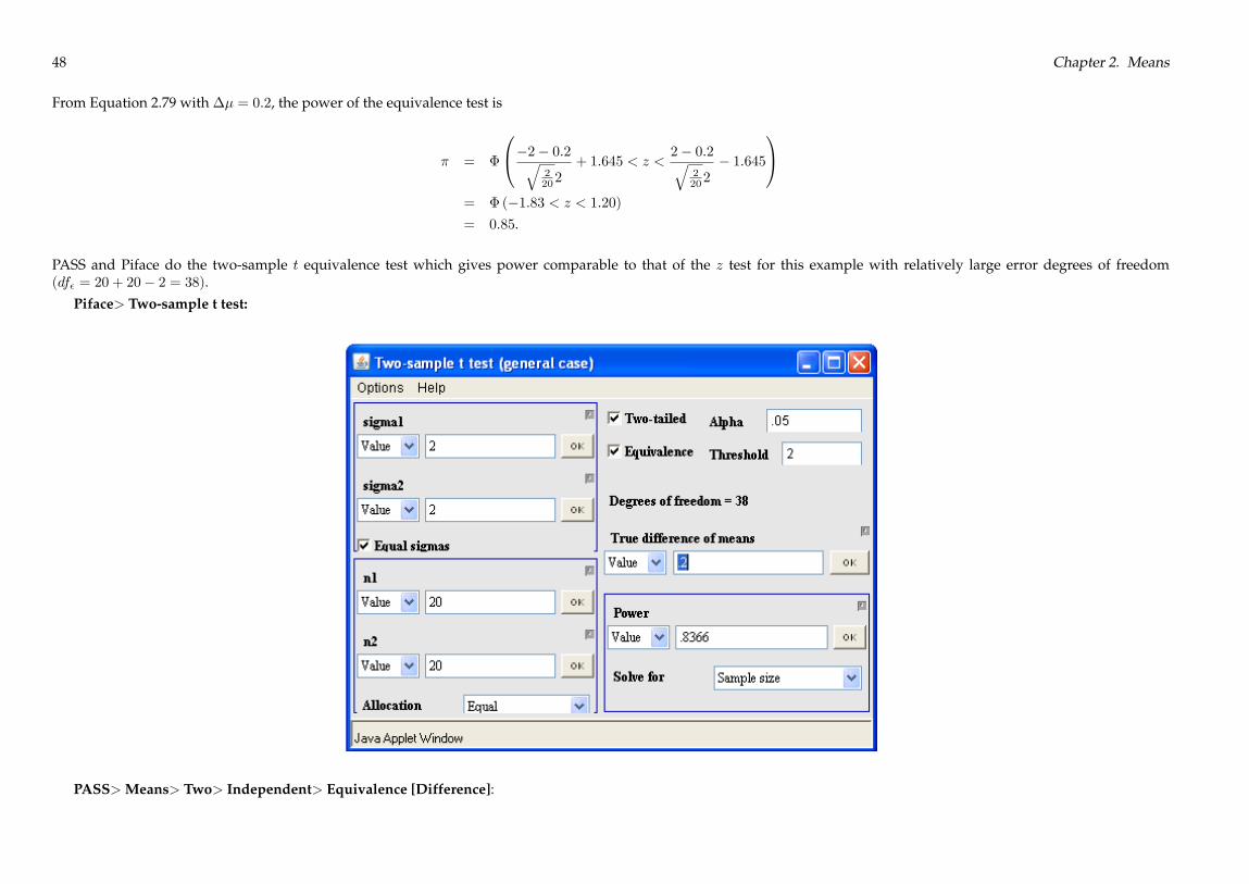
Example 2.13 Determine the power of the two independent-sample equivalence test where �1 and �2 are considered to be practically equivalent if j��j < 2 when �� = 0:2,�1 = �2 = 2, and n1 = n2 = 20.Solution: With � = 2 as the limit of practical equivalence, the hypotheses to be tested are
H01 : �� � �2 versus HA1 : �� > �2H02 : �� � 2 versus HA2 : �� < 2.
48 Chapter 2. Means
From Equation 2.79 with�� = 0:2, the power of the equivalence test is
� = �
0@�2� 0:2q2202
+ 1:645 < z <2� 0:2q
2202
� 1:645
1A= �(�1:83 < z < 1:20)= 0:85.
PASS and Piface do the two-sample t equivalence test which gives power comparable to that of the z test for this example with relatively large error degrees of freedom(df� = 20 + 20� 2 = 38).
Piface> Two-sample t test:
PASS>Means> Two> Independent> Equivalence [Difference]:
2.4. Equivalence Tests 49
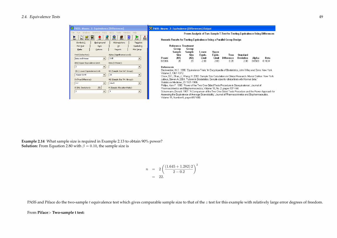
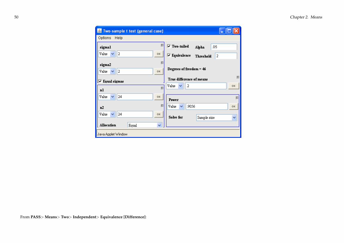
Example 2.14 What sample size is required in Example 2.13 to obtain 90% power?Solution: From Equation 2.80 with � = 0:10, the sample size is
n = 2
�(1:645 + 1:282) 2
2� 0:2
�2= 22.
PASS and Piface do the two-sample t equivalence test which gives comparable sample size to that of the z test for this example with relatively large error degrees of freedom.
From Piface> Two-sample t test:
50 Chapter 2. Means
From PASS>Means> Two> Independent> Equivalence [Difference]:
2.5. Contrasts 51
2.5 Contrasts
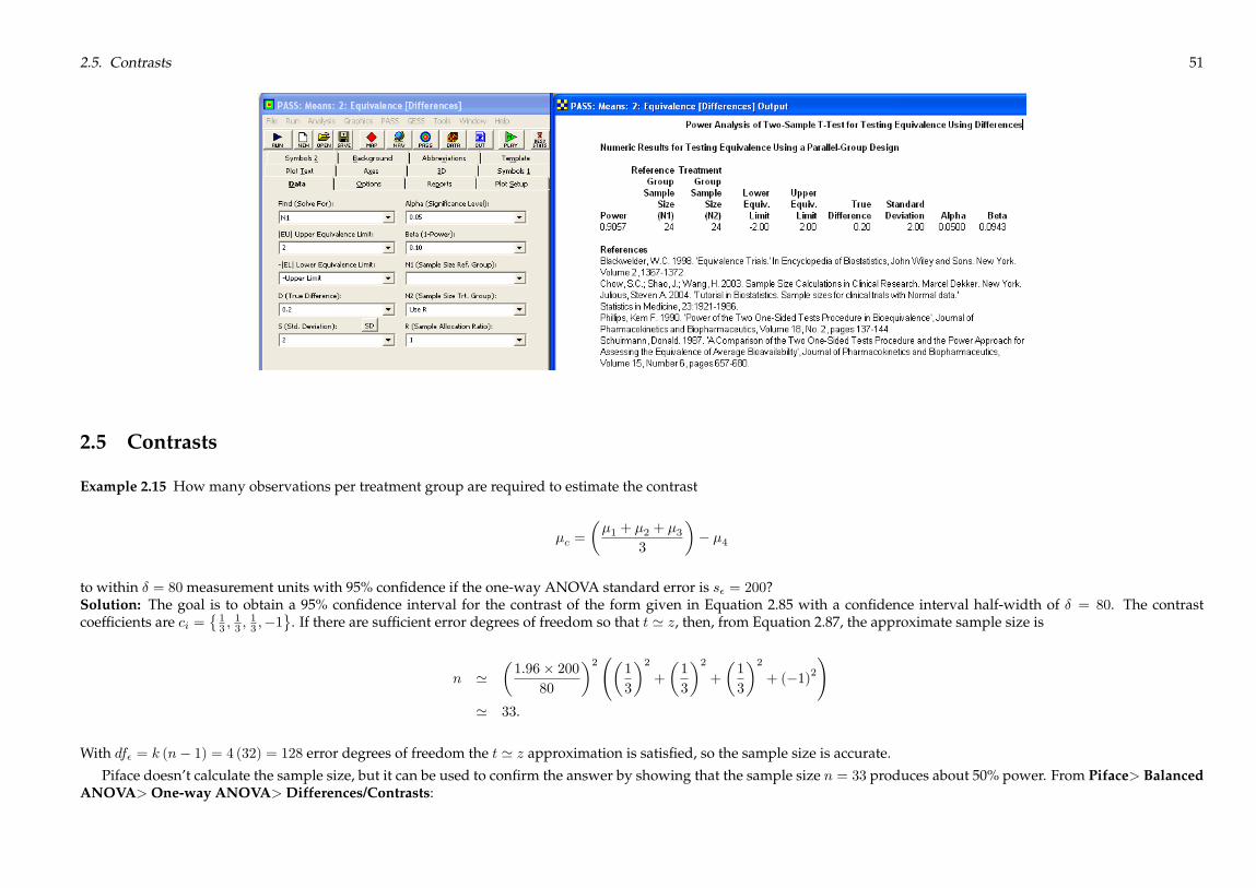
Example 2.15 How many observations per treatment group are required to estimate the contrast
�c =
��1 + �2 + �3
3
�� �4
to within � = 80 measurement units with 95% confidence if the one-way ANOVA standard error is s� = 200?Solution: The goal is to obtain a 95% confidence interval for the contrast of the form given in Equation 2.85 with a confidence interval half-width of � = 80. The contrastcoefficients are ci =
�13 ;
13 ;
13 ;�1
. If there are sufficient error degrees of freedom so that t ' z, then, from Equation 2.87, the approximate sample size is
n '�1:96� 200
80
�2 �1
3
�2+
�1
3
�2+
�1
3
�2+ (�1)2
!' 33.
With df� = k (n� 1) = 4 (32) = 128 error degrees of freedom the t ' z approximation is satisfied, so the sample size is accurate.
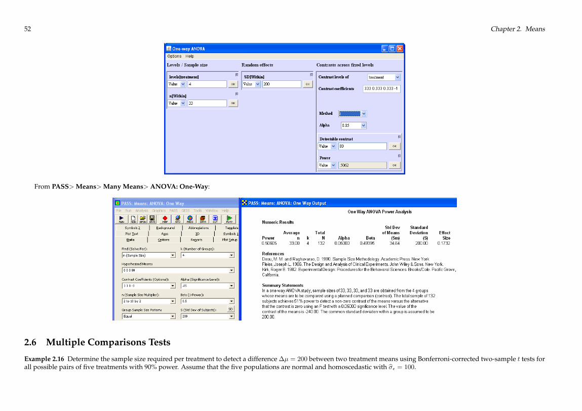
Piface doesn’t calculate the sample size, but it can be used to confirm the answer by showing that the sample size n = 33 produces about 50% power. From Piface> BalancedANOVA>One-way ANOVA>Differences/Contrasts:
52 Chapter 2. Means
From PASS>Means>Many Means> ANOVA: One-Way:
2.6 Multiple Comparisons Tests
Example 2.16 Determine the sample size required per treatment to detect a difference�� = 200 between two treatment means using Bonferroni-corrected two-sample t tests forall possible pairs of five treatments with 90% power. Assume that the five populations are normal and homoscedastic with b�� = 100.

2.6. Multiple Comparisons Tests 53
Solution: With k = 5 treatments there will be K =�52
�= 10 two-sample t tests to perform. To restrict the family error rate to �family = 0:05, the Bonferroni-corrected error rate
for individual tests is
� =0:05
10= 0:005.
By Equation 2.62 with t ' z, the sample size is
n = 2
�(z0:0025 + z0:10) b��
�
�2= 2
�(2:81 + 1:282) 100
200
�2= 9.
There will be df� = dftotal � dfmodel = (5� 9� 1) � (4) = 40 degrees of freedom to estimate b�� from the pooled treatment standard deviations, so the approximation t ' z isjustified.
From Piface> Balanced ANOVA>One-way ANOVA>Differences/Contrasts:
PASS uses a more conservative method for analyzing multiple comparisons which gives a larger sample size.
Example 2.17 Determine the approximate power for the sample size calculated in Example 2.16.
54 Chapter 2. Means
Solution: The approximate power for the test is given by Equations 2.58 and 2.60 with � = 0:005:
� = P (�1 < t < t�)
= P
��1 < t <
�rn
2
��b� � t�=2��
= P
�1 < t <
r9
2
200
100� t0:0025;40
!!= P (�1 < t < 1:273)
= 0:895.
Example 2.18 Bonferroni’s method becomes very conservative when the number of tests gets very large. A less conservative method for determining � for individual tests isgiven by Sidak’s method:
� = 1� (1� �family)1=K . (2.93)
Compare the sample sizes determined using Bonferroni’s and Sidak’s methods for multiple comparisons between all possible pairs of fifteen treatments when the tests mustdetect a difference of�� = 8with 90% power when b�� = 6.Solution: The number of multiple comparisons tests required is �
15
2
�=15� 142
= 105.
By Bonferroni’s method with �family = 0:05, the � for individual tests is
� =0:05
105= 0:000476,
so with t ' z in Equation 2.62 the sample size is
n = 2
�z0:000476=2 + z0:10
� b���
!2
= 2
�(3:494 + 1:282) 6
8
�2= 26.
By Sidak’s method (Equation 2.63), the � for individual tests is� = 1� (1� 0:05)1=105 = 0:000488,
so the sample size is
n = 2
�z0:000488=2 + z0:10
� b���
!2
= 2
�(3:487 + 1:282) 6
8
�2= 26.
Even with over 100 multiple comparisons, the sample sizes by the two calculation methods are still equal.

2.6. Multiple Comparisons Tests 55
Example 2.19 An experiment will be performed to compare four treatment groups to a control group. Determine the sample size required to detect a difference � = 200 betweenthe treatments and the control using Bonferroni-corrected two-sample t tests with 90% power. Use a balanced design with the same number of observations in each of the fivegroups and assume that the five populations are normal and homoscedastic with b�� = 100.Solution: To restrict the family error rate to �family = 0:05 withK = 4 tests, the Bonferroni-corrected error rate for individual tests is
� =0:05
4= 0:0125.
By Equation 2.62 with t ' z, the sample size is
n = 2
�z0:0125=2 + z0:10
� b���
!2
= 2
�(2:50 + 1:282) 100
200
�2= 8.
Despite the small treatment-group sample size, the approximation t ' z is justified because there will be df� = dftotal � dfmodel = (5� 8� 1) � (4) = 35 degrees of freedom toestimate b�� from the five pooled treatment standard deviations.
Piface offers Dunnett’s test, but it uses the Bonferroni correction to approximate Dunnett’s method so it gives the same result. From Piface> Balanced ANOVA> One-wayANOVA>Differences/Contrasts:
Example 2.20 Repeat Example 2.19 using the optimal allocation of units to treatments and controls.Solution: From Equation 2.98 with t ' z andK = 4,
ni =
�1 +
1p4
��(2:50 + 1:282) 100
200
�2= 6

56 Chapter 2. Means
andn0 = ni
pK = 6
p4 = 12.
The approximation t ' z is still justified because the error degrees of freedom will be df� = (4� 6 + 12) � 4 = 32. The original experiment required 5 � 8 = 40 units, but theoptimal experiment requires only 4� 6 + 12 = 36 units to obtain the same power.

Chapter 3
Standard Deviations
3.1 One Standard Deviation
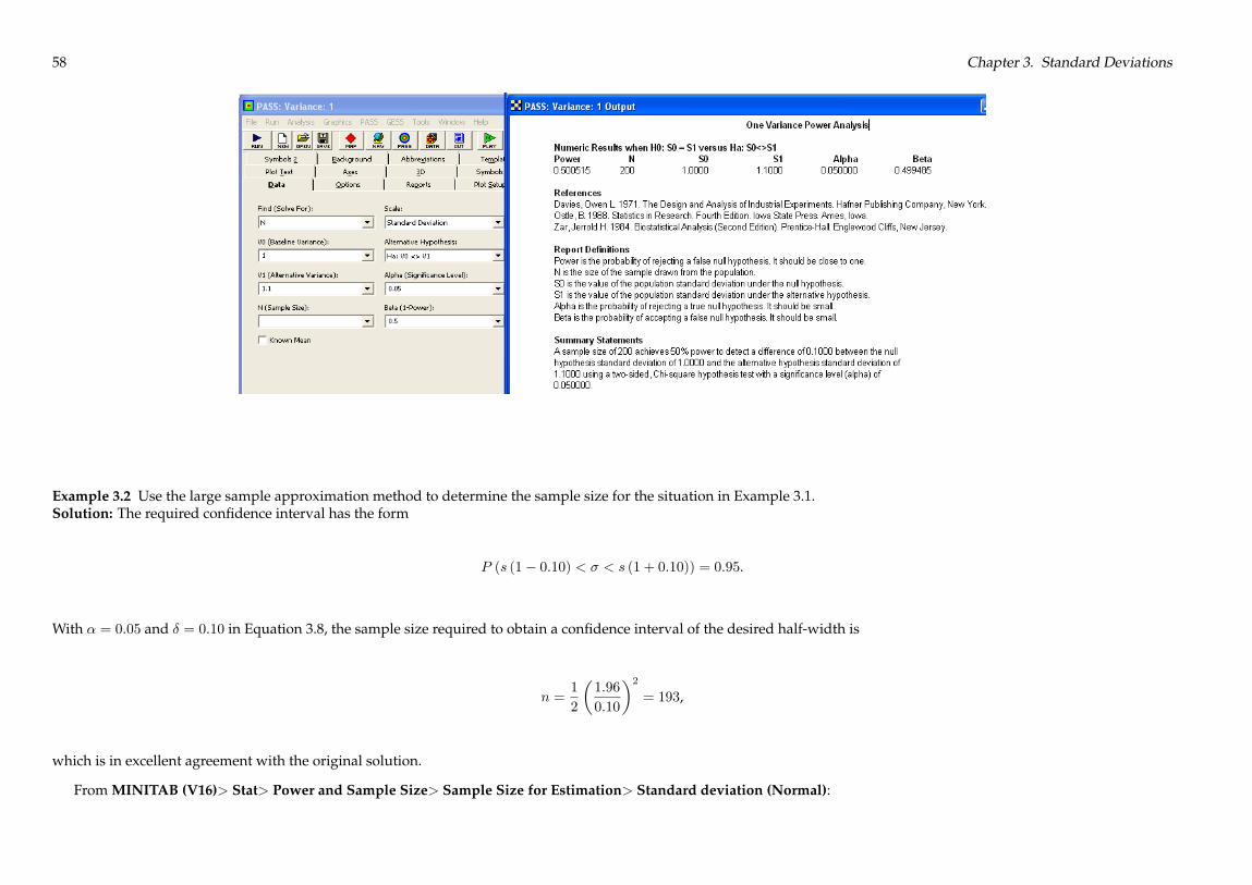
Example 3.1 Determine the sample size required to construct the 95% confidence interval for � based on a random sample of size n drawn from a normal population if theconfidence interval half-width must be about 10% of the sample standard deviation.Solution: From Table 3.1 the sample size must be about n = 200. The lower and upper confidence limits will fall at about -9% and +11% relative to the sample standard deviation,so the asymmetry for this relatively large sample size is not too severe.
From PASS> Variance> Variance: 1 Group (Note that when the Scale text box is set to Standard Deviation, other text boxes on the form with labels that refer to variances areinterpreted as standard deviations.):
57
58 Chapter 3. Standard Deviations
Example 3.2 Use the large sample approximation method to determine the sample size for the situation in Example 3.1.Solution: The required confidence interval has the form
P (s (1� 0:10) < � < s (1 + 0:10)) = 0:95.
With � = 0:05 and � = 0:10 in Equation 3.8, the sample size required to obtain a confidence interval of the desired half-width is
n =1
2
�1:96
0:10
�2= 193,
which is in excellent agreement with the original solution.
From MINITAB (V16)> Stat> Power and Sample Size> Sample Size for Estimation> Standard deviation (Normal):

3.1. One Standard Deviation 59
Example 3.3 For the test of H0 : �2 = 10 versus HA : �2 > 10, find the power associated with �2 = 20 when the sample size is n = 20 using � = 0:05.Solution: From Equation 3.14 the power is given by
� = P
��20:95
�10
20
�< �2 <1
�= P
�15:1 < �2 <1
�= 0:72.
From MINITAB (V16)> Stat> Power and Sample Size> 1 Variance:
From PASS> Variance> Variance: 1 Group:

60 Chapter 3. Standard Deviations
Example 3.4 Find the sample size required to reject H0 : �2 = 40with 90% power when �2 = 100 using HA : �2 > 40with � = 0:05.Solution: From Equation 3.15 with �20 = 40 and �21 = 100, the necessary sample size is the smallest value of n that meets the requirement
�20:95�20:10
� 100
40
� 2:5.
By inspecting Table 3.2 and a table of �2 values, the required sample size is n = 22 for which��20:95�20:10
=32:67
13:24= 2:469
�� 2:5.
From MINITAB (V16)> Stat> Power and Sample Size> 1 Variance:

3.1. One Standard Deviation 61
From PASS> Variance> Variance: 1 Group:
Example 3.5 Find the sample size required to reject H0 : � = 0:003 in favor of HA : � < 0:003with 90% power when in fact � = 0:001.Solution: With � = 0:05 and � = 1� � = 0:10, the sample size condition given by Equation 3.17 is
�20:90�20:05
��0:003
0:001
�2� 9:0,
which, from Table 3.2, is satisfied by n = 5.
From MINITAB (V16)> Stat> Power and Sample Size> 1 Variance:
From PASS> Variance> Variance: 1 Group:

62 Chapter 3. Standard Deviations
Example 3.6 Compare the power determined by the large-sample approximation method to the exact power determined in Example 3.3.Solution: The null hypothesis may be written as H0 : ln (�) = ln
�p10�
and we wish to find the power to reject H0 when ln(�) = ln�p20�
with n = 20. From Equation 3.20 wehave
z� =p2� 20 ln
r20
10
!� z0:05 = 0:547

3.2. Two Standard Deviations 63
and by Equation 3.19 the approximate power is
� = �(�0:547 < z <1)= 0:71.
This result is still in good agreement with the exact power of 72% despite the rather small sample size.
Example 3.7 Compare the sample size determined by the large-sample approximation method to the exact sample size determined in Example 3.4.Solution: The problem is to find the sample size to reject H0 : ln (�) = ln
�p40�
with 90% power when ln (�) = ln�p100�. With � = 0:05 and � = 0:10 in Equation ?? the
approximate sample size required is
n =1
2
0B@1:645 + 1:282ln�q
10040
�1CA2
= 21,
which is in good agreement with the exact sample size of n = 22.
3.2 Two Standard Deviations
Example 3.8 What equal-n sample size is required by an experiment to deliver a confidence interval for the ratio of two independent population standard deviations if the trueratio should fall within 20% of the experimental ratio with 95% confidence?Solution: The goal of the experiment is to determine an interval of the form
P
�s1s2(1� 0:2) < �1
�2<s1s2(1 + 0:2)
�= 1� �.
Then, from Equation ?? with � = 0:2, the required sample sizes are
n1 = n2 =�z0:025
�
�2=
�1:96
0:20
�2= 97.
Piface and PASS support the F test for two variances which can be tricked into confirming the sample size for the confidence interval. The confidence interval is asymmetricso the sample size is taken as the average of the sample sizes required for �2=�1 = 1:2 and �2=�1 = 0:8.
From Piface> Two Variances (F Test):From PASS> Variance> Variance: 2 Groups:
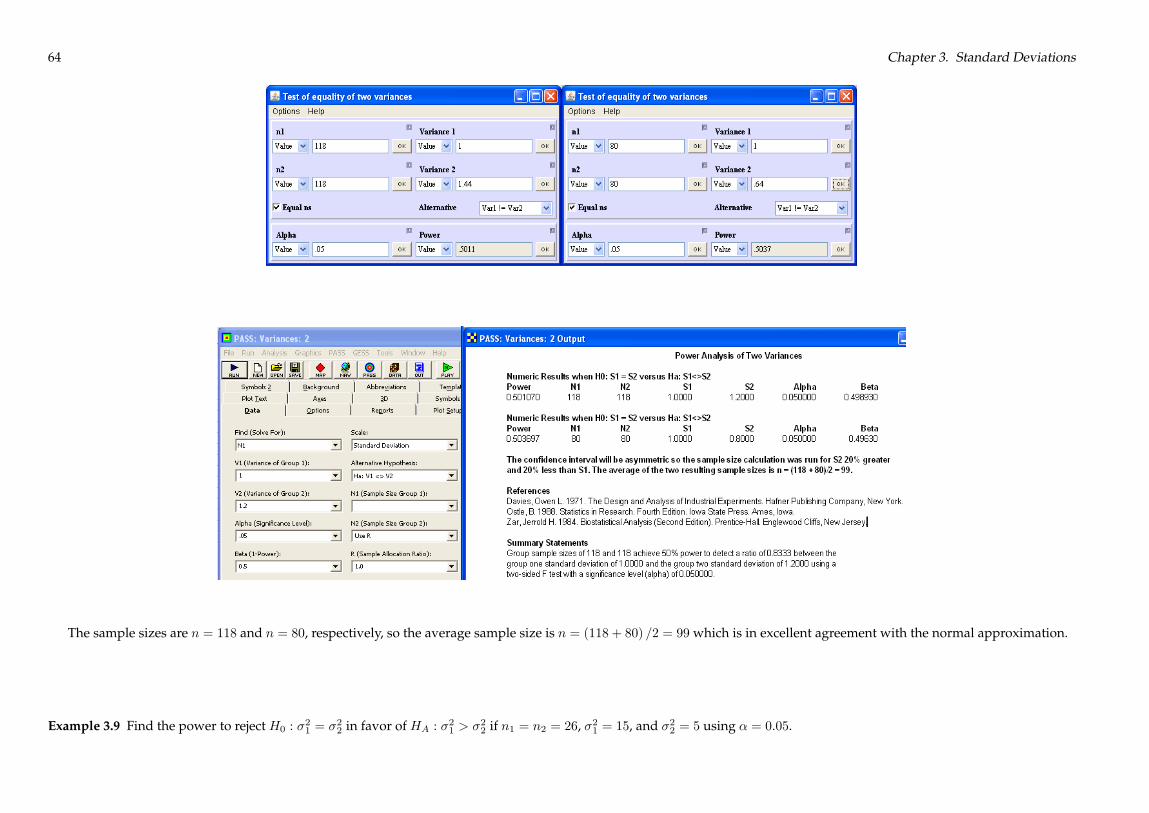
64 Chapter 3. Standard Deviations
The sample sizes are n = 118 and n = 80, respectively, so the average sample size is n = (118 + 80) =2 = 99 which is in excellent agreement with the normal approximation.
Example 3.9 Find the power to reject H0 : �21 = �22 in favor of HA : �21 > �22 if n1 = n2 = 26, �21 = 15, and �22 = 5 using � = 0:05.

3.2. Two Standard Deviations 65
Solution: From Equation 3.34 the power is
� = P
��2�1
�2F1�� < F <1
!
= P
��5
15
�F0:95;25;25 < F <1
�= P (0:652 < F <1)= 0:854.
From MINITAB (V16)> Stat> Power and Sample Size> 2 Variances:
From Piface> Two Variances (F Test):

66 Chapter 3. Standard Deviations
From PASS> Variance> Variance: 2 Groups:
Example 3.10 What equal sample size is required to detect a factor of two difference between two population standard deviations with 90% power and � = 0:05?

3.2. Two Standard Deviations 67
Solution: A factor of two difference in population standard deviation corresponds to a factor of four difference in variance, so we need to determine the sample size such that
P
�1
4F1�� < F <1
�= 0:90.
By iterating through several values of sample size, we find that when n1 = n2 = 20, F0:95;19;19 = 2:168 and F0:096 = 2:168=4 = 0:542, which satisfies the problem statement.From MINITAB (V16)> Stat> Power and Sample Size> 2 Variances:
From Piface> Two Variances (F Test):From PASS> Variance> Variance: 2 Groups:

68 Chapter 3. Standard Deviations
Example 3.11 Repeat Example 3.9 using the large-sample approximation method.Solution: From the information given in the example problem statement
z� =ln�q
155
�q
12
�126 +
126
� � 1:645 = 1:16so the power is
� = �(�1:16 < z <1) = 0:877,which is in good agreement with the exact solution of � = 0:854.
Example 3.12 Repeat Example 3.10 using the large-sample approximation method.Solution: From the information given in the example problem statement
n1 = n2 =
�1:645 + 1:282
ln (2)
�2= 18,
which slightly underestimates the exact solution n = 20.
3.3 Coefficient of Variation
Example 3.13 Determine the sample size required to estimate the population coefficient of variation to within�25% with 95% confidence if the coefficient of variation is expectedto be about 30%.
3.3. Coefficient of Variation 69
Solution: With � = 0:05, � = 0:25, and dCV = 0:3 in Equation 3.45, the sample size must be
n =
�1:96
0:25
�2�(0:3)
2+1
2
�= 37.
Example 3.14 Determine the sample size required to reject H0 : CV = 0:5with 90% power when CV = 0:8.Solution: With CV0 = 0:5, CV1 = 0:8, � = 0:05, and � = 0:10 in Equation 3.49, the required sample size is
n =
0@1:96� 0:5q(0:5)
2+ 1
2 + 1:282� 0:8q(0:8)
2+ 1
2
0:8� 0:5
1A2
= 42.
Example 3.15 Determine the sample size required to reject H0 : CV1 = CV2 in favor of HA : CV1 6= CV2 with 90% power when CV1 = 0:3 and CV2 = 0:5.Solution: With CV1 = 0:3, CV2 = 0:5, � = 0:05, and � = 0:10 in Equation 3.57, the required sample size is
n =
0@1:96� 0:3q(0:3)
2+ 1
2 + 1:282� 0:5q(0:5)
2+ 1
2
0:3� 0:5
1A2
= 26.

70 Chapter 3. Standard Deviations

Chapter 4
Proportions
4.1 One Proportion (Large Population)
Example 4.1 How large a random sample is required to demonstrate that the fraction defective of a process is less than 1% with 95% confidence?Solution: The required confidence interval has the form
P (0 < p < 0:01) = 0:95
so pU = 0:01 and � = 0:05. If we assume that the sample size is small compared to the lot size, then Equation 4.4 can be used to approximate the sample size. However, becausethe number of defectives allowed in the sample was not specified, we must consider the possibility of different X values. For X = 0, by the rule of three (Equation 4.5), thesample size is
n ' 3
0:01' 300.
For X = 1, by Equation 4.4
n '�20:95;42 (0:01)
' 9:49
2 (0:01)
' 475.
The values of n can be found for other choices of X in a similar manner.Piface> CI for one proportion, PASS> Proportions> One Group> Confidence Interval - Proportion, and MINITAB> Stat> Power and Sample Size> 1 Proportion use
the normal approximation to the binomial distribution to calculate the sample size for a symmetric two-tailed confidence interval but the normal approximation isn’t valid forthis problem.
71
72 Chapter 4. Proportions
Example 4.2 What fraction of a large population must be inspected and found to be free of defectives to be 95% confident that the population contains no more than tendefectives?Solution: The goal of the experiment is to demonstrate that the population defective count satisfies the confidence interval P (0 < S � 10) = 0:95. With X = 0 and � = 0:05 inEquation 4.7, the fraction of the population that will need to be inspected is
n
N' �20:95
2SU(4.1)
' 3
10(4.2)
' 0:30.
This result violates the small-sample approximation requirement that n� N , but it provides a good starting point for iterations toward a more accurate result. When n becomesa substantial fraction of N , use the method shown in Section 10.4.1.2 instead. (This example is re-solved using that method in Example 10.21.)
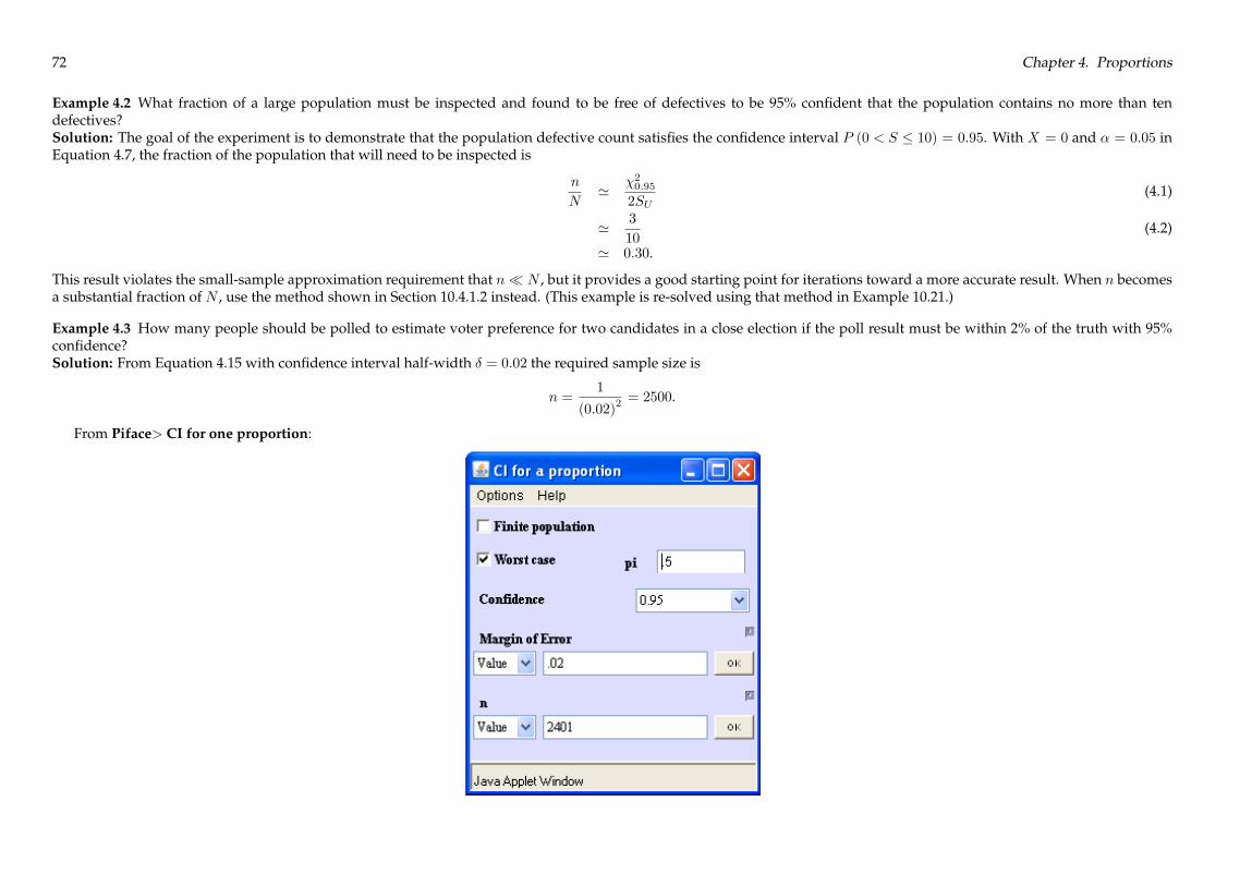
Example 4.3 How many people should be polled to estimate voter preference for two candidates in a close election if the poll result must be within 2% of the truth with 95%confidence?Solution: From Equation 4.15 with confidence interval half-width � = 0:02 the required sample size is
n =1
(0:02)2 = 2500.
From Piface> CI for one proportion:

4.1. One Proportion (Large Population) 73
From MINITAB (V16)> Stat> Power and Sample Size> Sample Size for Estimation> Proportion (Binomial):
From PASS> Proportions>One Group> Confidence Interval - Proportion:
From MINITAB> Stat> Power and Sample Size> 1 Proportion

74 Chapter 4. Proportions
Example 4.4 Find the power to reject H0 : p = 0:1when in fact p = 0:2 and the sample will be of size n = 200.Solution: Under bothH0 andHA the sample size is sufficiently large to justify the use of normal approximations to the binomial distributions. From Equation 4.21 with � = 0:05we have
z� =
p200 j0:2� 0:1j � z0:025
p(0:1) (1� 0:1)p
(0:2) (1� 0:2)= 2:066,
so the power is
� = 1� � (�1 < z < 2:066)
= 0:981.
From Piface> Test of one proportion:

4.1. One Proportion (Large Population) 75
From PASS> Proportions>One Group> Inequality [Differences]:
76 Chapter 4. Proportions
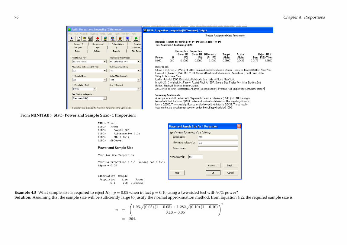
From MINITAB> Stat> Power and Sample Size> 1 Proportion:
Example 4.5 What sample size is required to reject H0 : p = 0:05 when in fact p = 0:10 using a two-sided test with 90% power?Solution: Assuming that the sample size will be sufficiently large to justify the normal approximation method, from Equation 4.22 the required sample size is
n =
1:96
p(0:05) (1� 0:05) + 1:282
p(0:10) (1� 0:10)
0:10� 0:05
!2= 264.

4.1. One Proportion (Large Population) 77
From Piface> Test of one proportion:
From PASS> Proportions>One Group> Inequality [Differences]:

78 Chapter 4. Proportions
From MINITAB> Power and Sample Size> 1 Proportion:
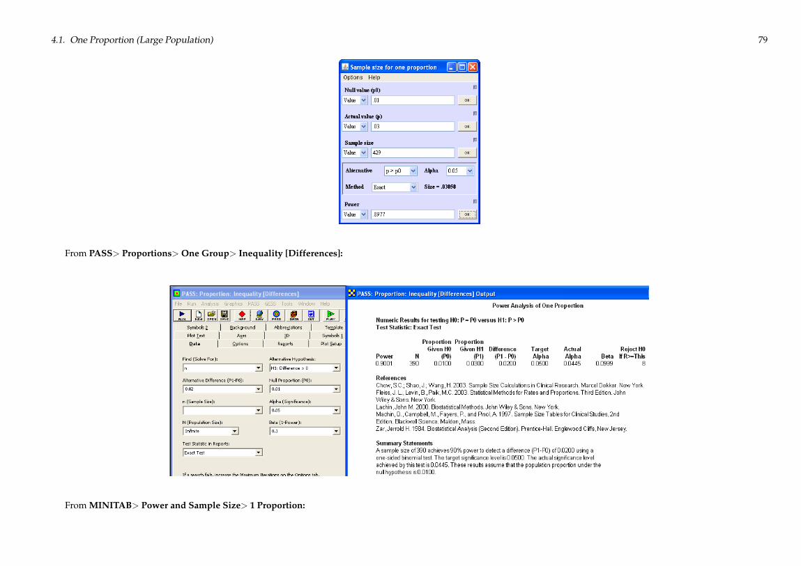
Example 4.6 What sample size is required to reject H0 : p = 0:01 with 90% power when in fact p = 0:03?Solution: The hypotheses to be tested areH0 : p = 0:01 versusHA : p > 0:01 and the two points on the OC curve are (p0; 1� �) = (0:01; 0:95) and (p1; �) = (0:03; 0:10). The exactsimultaneous solution to Equations 4.24 and 4.25, obtained using Larson’s nomogram and then iterating to the exact solution using a binomial calculator, is (n; c) = (390; 7). Thedistributions of the success counts under H0 and HA are shown in Figure 4.2.
From Piface> Test of one proportion:
4.1. One Proportion (Large Population) 79
From PASS> Proportions>One Group> Inequality [Differences]:
From MINITAB> Power and Sample Size> 1 Proportion:

80 Chapter 4. Proportions
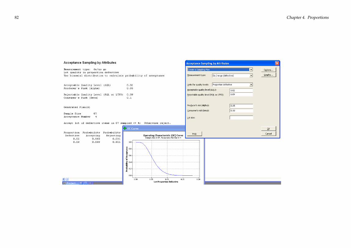
Example 4.7 Use Larson’s nomogram to find n and c for the sampling plan for defectives that will accept 95% of lots with 2% defectives and 10% of lots with 8% defectives.Draw the OC curve.Solution: Figure 4.3 shows the solution using Larson’s nomogram with the two specified points on the OC curve at (p; PA (H0)) = (0:02; 0:95) and (0:09; 0:10). The requiredsampling plan is n = 100 and c = 4. The OC curve is shown in Figure 4.4. Points on the OC were obtained by rocking a line about the point at n = 100 and c = 4 in the nomogramand reading off p and PA values.
From Piface> Test of one proportion:
From PASS> Proportions>One Group> Inequality [Differences]:

4.1. One Proportion (Large Population) 81
From MINITAB> Stat> Power and Sample Size> 1 Proportion:
From MINITAB> Stat>Quality Tools> Acceptance Sampling by Attributes:
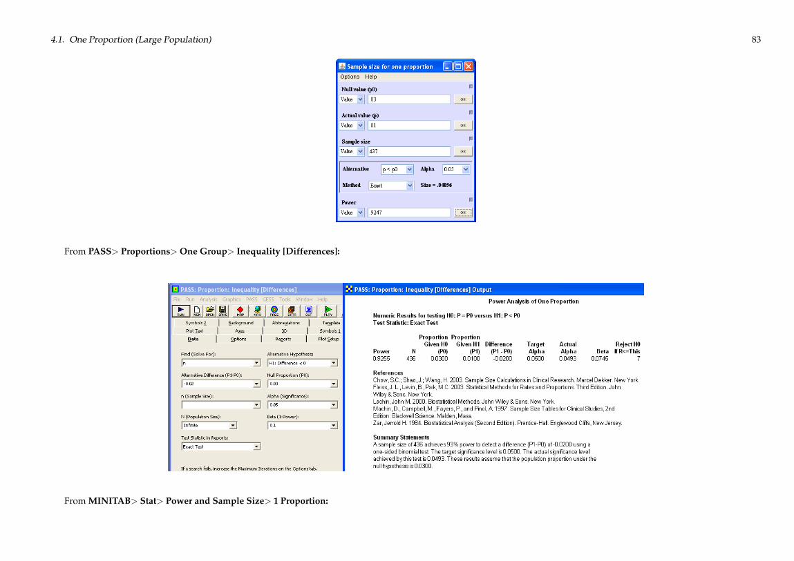
Example 4.8 What sample size is required to reject H0 : p = 0:03 with 90% power when in fact p = 0:01?Solution: The hypotheses to be tested are H0 : p = p0 versus HA : p < p0 and the two points on the OC curve are (p0; 1� �) = (0:03; 0:95) and (p1; �) = (0:01; 0:10). The exactsimultaneous solution to Equations 4.26 and 4.27, determined using Larson’s nomogram followed by manual iterations with a binomial calculator, is (n; r) = (436; 7).
From Piface> Test of one proportion:
82 Chapter 4. Proportions
4.1. One Proportion (Large Population) 83
From PASS> Proportions>One Group> Inequality [Differences]:
From MINITAB> Stat> Power and Sample Size> 1 Proportion:

84 Chapter 4. Proportions
From MINITAB> Stat>Quality Tools> Acceptance Sampling by Attributes:

4.2. One Proportion (Small Population) 85
4.2 One Proportion (Small Population)
Example 4.9 Suppose that a sample of size n = 20 drawn from a population of N = 100 units was found to have X = 2 defective units. Determine the one-sided upperconfidence limit for the population fraction defective.Solution: From the following hypergeometric probabilities:
h (0 � x � 2;S = 26; N = 100; n = 20) = 0:0555
h (0 � x � 2;S = 27; N = 100; n = 20) = 0:0448
the smallest value of S that satisfies the inequality in Equation 4.34 is S = 27, so the 95% one-sided upper confidence limit for S is SU = 27 or
P (S � 27) � 0:95.

86 Chapter 4. Proportions
Example 4.10 A hospital is asked by an auditor to confirm that its billing error rate is less than 10% for a day chosen randomly by the auditor. However, it is impractical toinspect all 120 bills issued on that day. How many of the bills must be inspected to demonstrate, with 95% confidence, that the billing error rate is less than 10%?Solution: The goal of the analysis is to demonstrate that the one-sided upper 95% confidence limit on the billing error rate p is 10% or
P (p � 0:10) = 0:95.
Under the assumption that the auditor will accept a zero defectives sampling plan, by the rule of three (Equation 4.5) the approximate sample size must be
n ' 3
p=
3
0:10= 30.
Because n = 30 is large compared to N = 120, the finite population correction factor (Equation 4.16) should be used and gives
n0 =30
1 + 30�1120
= 25.
Iterations with a hypergeometric probability calculator show that n = 26 is the smallest sample size that gives 95% confidence that the billing error rate is less than 10%.
Example 4.11 What sample size nmust be drawn from a population of sizeN = 200 and found to be free of defectives if we need to demonstrate,with 95% confidence, that thereare no more than four defectives in the population?Solution: The goal of the experiment is to demonstrate the confidence interval
P (0 � S � 4) � 0:95
using a zero-successes (X = 0) sampling plan. By the small-sample binomial approximation with SU = 4 and � = 0:05, the required sample size by Equation 4.40 is given by
n =ln (0:05)
ln�1� 4
200
� = 149,which violates the small-sample assumption. By Equation 4.42, the rare-event binomial approximation gives
n � N�1� �1=SU
�� 200
�1� 0:051=4
�� 106.
This solution meets the requirements of the rare-event approximation method, but just to check this result, the corresponding exact hypergeometric probability is h (0; 4; 200; 106) =0:047which is less than � = 0:05 as required, however, because h (0; 4; 200; 105) = 0:049, the sample size n = 105 is the exact solution to the problem.
4.2. One Proportion (Small Population) 87
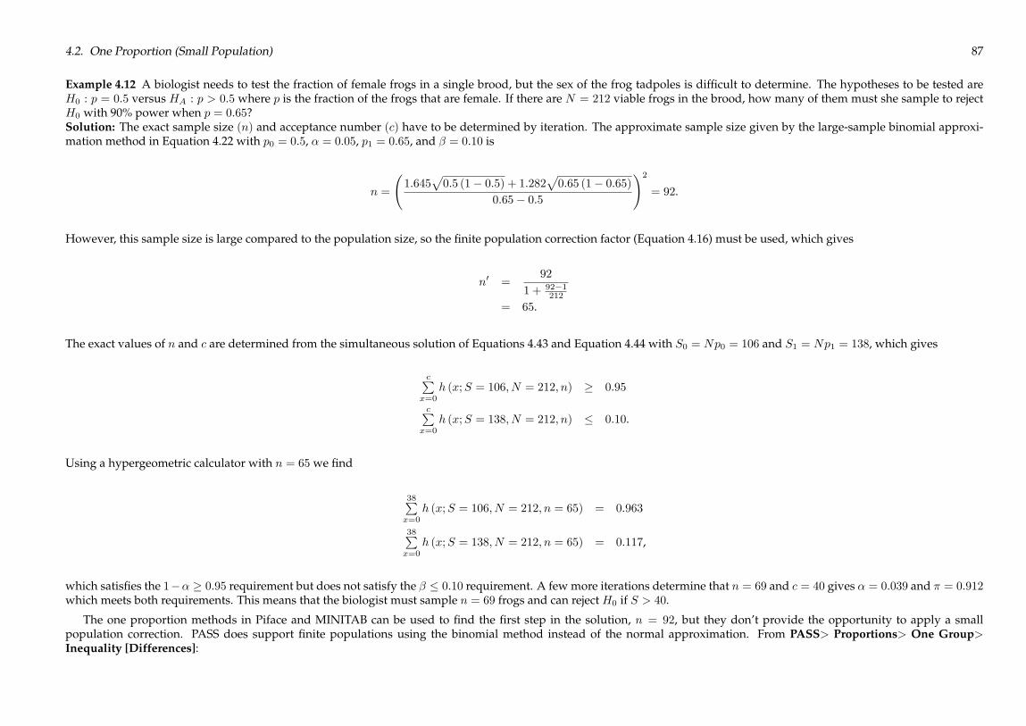
Example 4.12 A biologist needs to test the fraction of female frogs in a single brood, but the sex of the frog tadpoles is difficult to determine. The hypotheses to be tested areH0 : p = 0:5 versus HA : p > 0:5 where p is the fraction of the frogs that are female. If there are N = 212 viable frogs in the brood, how many of them must she sample to rejectH0 with 90% power when p = 0:65?Solution: The exact sample size (n) and acceptance number (c) have to be determined by iteration. The approximate sample size given by the large-sample binomial approxi-mation method in Equation 4.22 with p0 = 0:5, � = 0:05, p1 = 0:65, and � = 0:10 is
n =
1:645
p0:5 (1� 0:5) + 1:282
p0:65 (1� 0:65)
0:65� 0:5
!2= 92.
However, this sample size is large compared to the population size, so the finite population correction factor (Equation 4.16) must be used, which gives
n0 =92
1 + 92�1212
= 65.
The exact values of n and c are determined from the simultaneous solution of Equations 4.43 and Equation 4.44 with S0 = Np0 = 106 and S1 = Np1 = 138, which gives
cPx=0
h (x;S = 106; N = 212; n) � 0:95
cPx=0
h (x;S = 138; N = 212; n) � 0:10.
Using a hypergeometric calculator with n = 65 we find
38Px=0
h (x;S = 106; N = 212; n = 65) = 0:963
38Px=0
h (x;S = 138; N = 212; n = 65) = 0:117,
which satisfies the 1�� � 0:95 requirement but does not satisfy the � � 0:10 requirement. A few more iterations determine that n = 69 and c = 40 gives � = 0:039 and � = 0:912which meets both requirements. This means that the biologist must sample n = 69 frogs and can reject H0 if S > 40.
The one proportion methods in Piface and MINITAB can be used to find the first step in the solution, n = 92, but they don’t provide the opportunity to apply a smallpopulation correction. PASS does support finite populations using the binomial method instead of the normal approximation. From PASS> Proportions> One Group>Inequality [Differences]:
88 Chapter 4. Proportions
4.3 Two Proportions
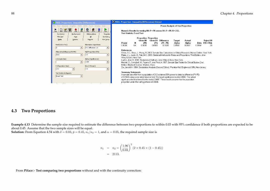
Example 4.13 Determine the sample size required to estimate the difference between two proportions to within 0.03 with 95% confidence if both proportions are expected to beabout 0.45. Assume that the two sample sizes will be equal.Solution: From Equation 4.54 with � = 0:03, �p = 0:45, n1=n2 = 1, and � = 0:05, the required sample size is
n1 = n2 =
�1:96
0:03
�2(2� 0:45� (1� 0:45))
= 2113.
From Piface> Test comparing two proportions without and with the continuity correction:
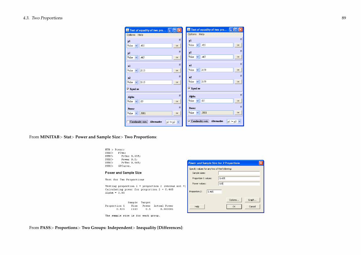
4.3. Two Proportions 89
From MINITAB> Stat> Power and Sample Size> Two Proportions:
From PASS> Proportions> Two Groups: Independent> Inequality [Differences]:

90 Chapter 4. Proportions
Example 4.14 An experiment is planned to estimate the risk ratio. The two proportions are expected to be p1 ' 0:2 and p2 ' 0:05. Determine the optimal allocation ratio and thesample size required to determine the risk ratio to within 20% of its true value with 95% confidence?Solution: A 95% confidence interval for the risk ratio is required of the form in Equation 4.56. With p1 = 0:2 and p2 = 0:05, the anticipated value of the risk ratio is RR '0:2=0:05 = 4 and from Equation 4.62 the optimal sample size allocation ratio is
n1n2=
s0:05=0:95
0:2=0:8= 0:4588.
Then with � = 0:2 and � = 0:05 in Equation 4.61, the required sample size n1 is
n1 =
�1:96
0:2
�2�1� 0:20:2
+1� 0:050:05
(0:4588)
�= 1222
and the sample size n2 is
n2 =n1�n1n2
� = 1222
0:4588= 2664.
These sample sizes minimize the total number of samples required for the experiment.
Example 4.15 An experiment is planned to estimate the odds ratio. The two proportions are expected to be p1 ' 0:5 and p2 ' 0:25. Determine the optimal allocation ratio andthe sample size required to determine, with 90% confidence, the odds ratio to within 20% of its true value?

4.3. Two Proportions 91
Solution: The desired confidence interval has the form given by Equation 4.64 with � = 0:2. With p1 = 0:5 and p2 = 0:25, the anticipated value of the odds ratio is OR =0:5=0:50:25=0:75 = 3 and from Equation 4.70 the optimal sample size allocation ratio is
n1n2=
r0:25� 0:750:5� 0:5 = 0:866.
Then with � = 0:2 and � = 0:10 in Equation 4.69, the required sample size n1 is
n1 =
�1:645
0:2
�2�1
0:5� 0:5 +1
0:25� 0:75 (0:866)�
= 584
and the sample size n2 is
n2 =n1�n1n2
� = 584
0:866= 675.
Example 4.16 Determine the power for Fisher’s test to reject H0 : p1 = p2 in favor of HA : p1 < p2 when p1 = 0:01, p2 = 0:50, and n1 = n2 = 8.Solution: The Fisher’s test p values for all possible combinations of x1 and x2 were calculated using Equation 4.71 and are shown in Table 4.3. The few cases that are statisticallysignificant, where p � 0:05, are shown in a bold font in the upper right corner of the table. Table 4.4 shows the contributions to the power given by the product of the twobinomial probabilities in Equation 4.74. The sum of the individual contributions, that is, the power of Fisher’s test, is � = 0:60.
From PASS> Proportions> Two Groups: Independent> Inequality [Differences]:
92 Chapter 4. Proportions
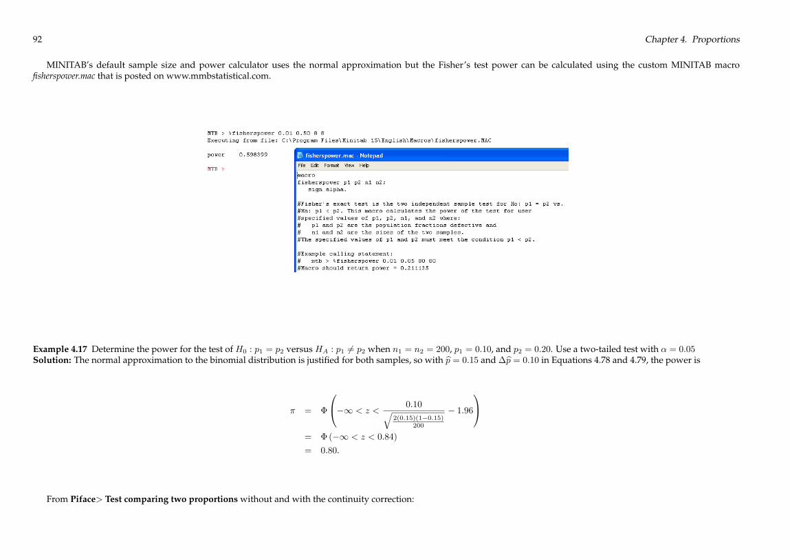
MINITAB’s default sample size and power calculator uses the normal approximation but the Fisher’s test power can be calculated using the custom MINITAB macrofisherspower.mac that is posted on www.mmbstatistical.com.
Example 4.17 Determine the power for the test of H0 : p1 = p2 versus HA : p1 6= p2 when n1 = n2 = 200, p1 = 0:10, and p2 = 0:20. Use a two-tailed test with � = 0:05Solution: The normal approximation to the binomial distribution is justified for both samples, so with bp = 0:15 and �bp = 0:10 in Equations 4.78 and 4.79, the power is
� = �
0@�1 < z <0:10q
2(0:15)(1�0:15)200
� 1:96
1A= �(�1 < z < 0:84)
= 0:80.
From Piface> Test comparing two proportions without and with the continuity correction:
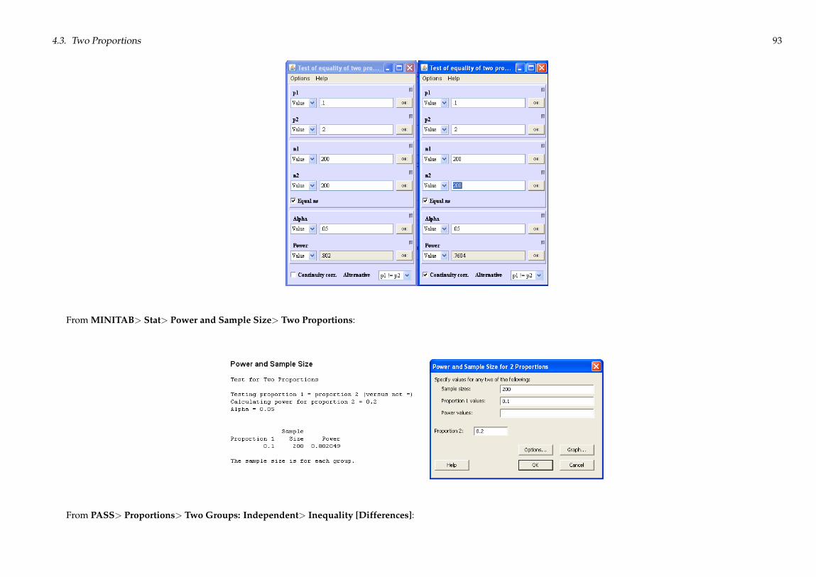
4.3. Two Proportions 93
From MINITAB> Stat> Power and Sample Size> Two Proportions:
From PASS> Proportions> Two Groups: Independent> Inequality [Differences]:

94 Chapter 4. Proportions
Example 4.18 What common sample size is required to resolve the difference between two proportions with 90% power using a two-sided test when p1 = 0:10 and p2 = 0:20 isexpected?Solution: From Equation 4.80 with bp = 0:15 and �bp = 0:10 the required sample size is
n =2� 0:15� 0:85
(0:10)2 (1:28 + 1:96)
2
= 268.
From Piface> Test comparing two proportions without the continuity correction:

4.3. Two Proportions 95
From MINITAB> Stat> Power and Sample Size> Two Proportions:
From PASS> Proportions> Two Groups: Independent> Inequality [Differences]:
96 Chapter 4. Proportions
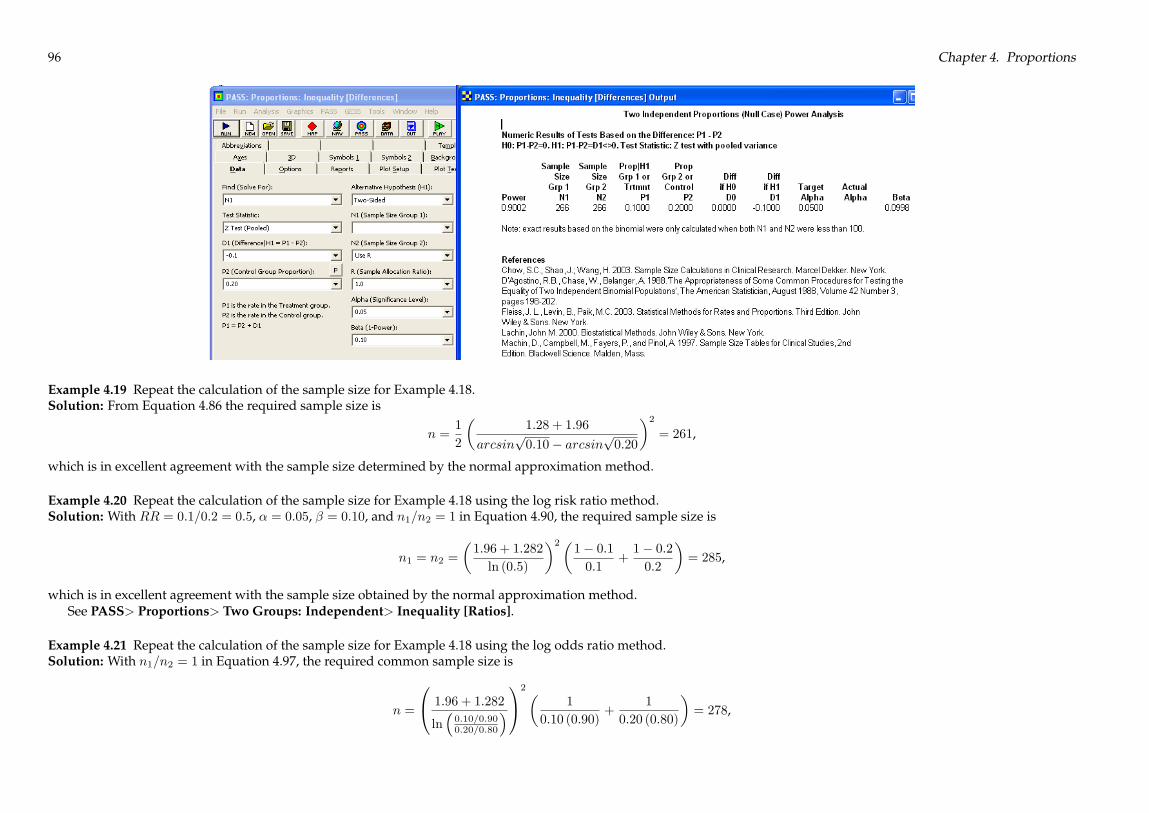
Example 4.19 Repeat the calculation of the sample size for Example 4.18.Solution: From Equation 4.86 the required sample size is
n =1
2
�1:28 + 1:96
arcsinp0:10� arcsin
p0:20
�2= 261,
which is in excellent agreement with the sample size determined by the normal approximation method.
Example 4.20 Repeat the calculation of the sample size for Example 4.18 using the log risk ratio method.Solution: With RR = 0:1=0:2 = 0:5, � = 0:05, � = 0:10, and n1=n2 = 1 in Equation 4.90, the required sample size is
n1 = n2 =
�1:96 + 1:282
ln (0:5)
�2�1� 0:10:1
+1� 0:20:2
�= 285,
which is in excellent agreement with the sample size obtained by the normal approximation method.See PASS> Proportions> Two Groups: Independent> Inequality [Ratios].
Example 4.21 Repeat the calculation of the sample size for Example 4.18 using the log odds ratio method.Solution: With n1=n2 = 1 in Equation 4.97, the required common sample size is
n =
0@ 1:96 + 1:282
ln�0:10=0:900:20=0:80
�1A2�
1
0:10 (0:90)+
1
0:20 (0:80)
�= 278,

4.3. Two Proportions 97
which is in excellent agreement with the sample size obtained by the normal approximation method.See PASS> Proportions> Two Groups: Independent> Inequality [Odds Ratios].
Example 4.22 Determine the number of subjects required for McNemar’s test to reject H0 : RR = 1 with 90% power when RR = 2 and the rate of discordant observations isestimated to be pD = 0:2 from a preliminary study.Solution: With � = 0:10 and � = 0:05 in Equation 4.105, the approximate number of subjects required for the study is
Pi
Pj
bfij ' (1:282 + 1:96)2
0:20
�2 + 1
2� 1
�2' 473.
From PASS> Proportions> Two Groups: Paired or Correlated> Inequality (McNemar) [Odds Ratios]:
Example 4.23 Determine the McNemar’s test power to reject H0 : RR = 1 in favor of HA : RR 6= 1 for a study with 200 subjects when in fact RR = 3 using pD = 0:3.Solution: With 200 subjects in the study, the expected number of discordant pairs is
bf12 + bf21 = pDPi
Pj
bfij = 0:3� 200 = 60.
Under HA with RR = 3, we have bf21 = 15 and bf12 = 45, so the expected value of the McNemar’s zM statistic is
zM =j45� 15jp45 + 15
= 3:87

98 Chapter 4. Proportions
and the approximate power is
� = P (�1 < z < z�)
= P��1 < z <
�zM � z�=2
��= P (�1 < z < (3:87� 1:96))= P (�1 < z < 1:91)
= 0:972.
From PASS> Proportions> Two Groups: Paired or Correlated> Inequality (McNemar) [Odds Ratios]:
4.4 Equivalence Tests
Example 4.24 For the test of H0 : p < 0:45 or p > 0:55 versus HA : 0:45 < p < 0:55, calculate the exact and approximate power when p = 0:5 assuming that the sample size isn = 800 and � = 0:05.Solution: The value of x1,determined from Equation 4.106, is x1 = 384 because
383Px=0
b (x;n = 800; p1 = 0:45) = 0:952.
The value of x2, determined from Equation 4.107, is x2 = 416 because
416Px=0
b (x;n = 800; p2 = 0:55) = 0:048.

4.4. Equivalence Tests 99
Then the power when p = 0:5 is given by Equation 4.108:
� =416P
x=383b (x;n = 800; p2 = 0:50)
= 0:757.
The approximate power by the normal approximation method, given by Equation 4.111, is
� = �
0@ 0:45� 0:5q0:5(1�0:5)
800
+ 1:645 < z <0:55� 0:5q0:5(1�0:5)
800
� 1:645
1A= �(�1:183 < z < 1:183)= 0:763,
which is in good agreement with the exact solution.From PASS> Proportions>One Group: Equivalence [Differences]:
Example 4.25 An experiment is to be performed to test the hypotheses H0 : p1 6= p2 versus HA : p1 = p2. The two proportions are expected to be p ' 0:12 and the limit ofpractical equivalence is � = 0:02. What sample size is required to reject H0 when p1 = p2 with 80% power?

100 Chapter 4. Proportions
Solution: With � = 0:05 and n1=n2 = 1 in Equation 4.118, the sample size n = n1 = n2 is
n = 2 (z0:05 + z0:10)2 0:12 (1� 0:12)
(0:02)2
= 2 (1:645 + 1:282)2 0:12 (1� 0:12)
(0:02)2
= 4524.
From PASS> Proportions> Two Groups: Independent> Equivalence [Differences]:
Example 4.26 What sample size is required if the true difference between the two proportions in Example4.254.25 is�p = 0:01?

4.4. Equivalence Tests 101
Solution: p1 and p2 are not specified, but they are both approximately p = 0:12, so from Equation 4.119 the sample size must be
n1 ' 2 (z� + z�)2 p (1� p)(� � j�pj)2
' 2 (1:645 + 0:842)2 0:12 (1� 0:12)(0:02� 0:01)2
' 13063.
From PASS> Proportions> Two Groups: Independent> Equivalence [Differences]:
102 Chapter 4. Proportions
4.5 Chi-square Tests
Example 4.27 Confirm the sample size for Example 4.18 using the �2 test method for a 2� 2 table.Solution: Under HA with p1 = 0:10 and p2 = 0:20 the expected proportion of observations in each cell of the 2� 2 table is
(pij)A =1
2
�0:1 0:90:2 0:8
�=
�0:05 0:450:1 0:4
�.
Under H0 with p1 = p2 = (0:1 + 0:2) =2 = 0:15 the expected distribution of observations is
(pij)0 =1
2
�0:15 0:850:15 0:85
�=
�0:075 0:4250:075 0:425
�.
From Equation 4.121 with a total of 2� 268 = 536 observations the noncentrality parameter is
� = 536
(0:05� 0:075)2
0:075+(0:1� 0:075)2
0:075+(0:45� 0:425)2
0:425
+(0:4� 0:425)2
0:425
!= 10:51.
Then, with � = 0:05 and df = 1 degree of freedom in Equation 4.122,�20:95 = 3:8415 = �
2�;10:51
which is satisfied by � = 0:10, so the power is � = 1� � = 0:90 and is consistent with the original example problem solution.
Example 4.28 A large school district intends to perform pass/fail testing of students from four large schools to test for performance differences among schools. If 50 studentsare chosen randomly from each school, what is the power of the �2 test to reject the null hypothesis of homogeneity when the student failure rates at the four schools are in fact10%, 10%, 10%, and 30%?Solution: To calculate the power of the �2 test we must specify the two 2� 4 tables (result by school) associated with (pij)0 and (pij)A. From the problem statement, under HAwith (p1j)A = f0:1; 0:1; 0:1; 0:3g, the table of (pij)A is
(pij)A =1
4
�0:1 0:1 0:1 0:30:9 0:9 0:9 0:7
�=
�0:025 0:025 0:025 0:0750:225 0:225 0:225 0:175
�.
The mean failure rate of all four schools is (3 (0:1) + 0:3) =4 = 0:15 under H0, so the corresponding table of (pij)0 is
(pij)0 =1
4
�0:15 0:15 0:15 0:150:85 0:85 0:85 0:85
�=
�0:0375 0:0375 0:0375 0:03750:2125 0:2125 0:2125 0:2125
�.

4.5. Chi-square Tests 103
Under these definitions, the �2 distribution noncentrality parameter is
� = 200
"3
(0:025� 0:0375)2
0:0375
!+(0:075� 0:0375)2
0:0375
+3
(0:225� 0:2125)2
0:2125
!+(0:175� 0:2125)2
0:2125
#= 11:77:
The �2 test statistic will have df = (2� 1) (4� 1) = 3 degrees of freedom, so the critical value of the test statistic is �20:95;3 = 7:81. The power of the test determined from thecondition
�20:95 = 7:81 = �21��;11:77
is � = 0:833.
From Piface>Generic chi-square test:
From PASS> Proportions>Multi-Group: Chi-Square Test with effect sizeW =p�=N =
p11:77=200 = 0:2425:

104 Chapter 4. Proportions
Example 4.29 What is the power to reject the claim that a die is balanced (H0 : �i = 16 for i = 1 to 6) when it is in fact slightly biased toward one die face (HA : �i =
f0:16; 0:16; 0:16; 0:16; 0:16; 0:20g) based on 100 rolls of the die?Solution: The table of observations will have six cells and there will be no parameters estimated from the sample data, so the �2 test will have df = 6� 1 = 5 degrees of freedom.From Equation 4.121 the noncentrality parameter will be
� = 100
"5
�0:16� 1
6
�216
!+
�0:20� 1
6
�16
#= 20:13.

4.5. Chi-square Tests 105
With � = 0:05 we have �20:95 = 11:07, so the power to reject H0 is determined from the condition
�20:95 = 11:07 = �21��;20:13,
which is satisfied by � = 0:954.From Piface>Generic chi-square test:
From PASS> Proportions>Multi-Group: Chi-Square Test with effect sizeW =p�=N =
p20:13=100 = 0:4487:

106 Chapter 4. Proportions

Chapter 5
Poisson Counts
5.1 One Poisson Count
Example 5.1 How many Poisson events must be observed if the relative error of the estimate for � must be no larger than �10% with 95% confidence?Solution: The desired confidence interval for � has the form
P�xn(1� 0:10) < � < x
n(1 + 0:10)
�= 0:95,
so � = 0:10 and from Equation 5.10
x =
�1:96
0:10
�2= 385.
That is, if the Poisson process is sampled until x = 385 counts are obtained, then the 95% confidence limits for � will be
UCL=LCL =
�385
n
�(1� 0:10)
or
P
�346
n< � <
424
n
�= 0:95.
From Piface>Generic Poisson test:
107
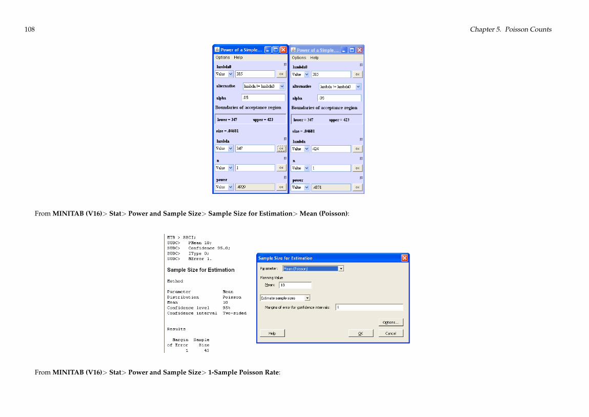
108 Chapter 5. Poisson Counts
From MINITAB (V16)> Stat> Power and Sample Size> Sample Size for Estimation>Mean (Poisson):
From MINITAB (V16)> Stat> Power and Sample Size> 1-Sample Poisson Rate:
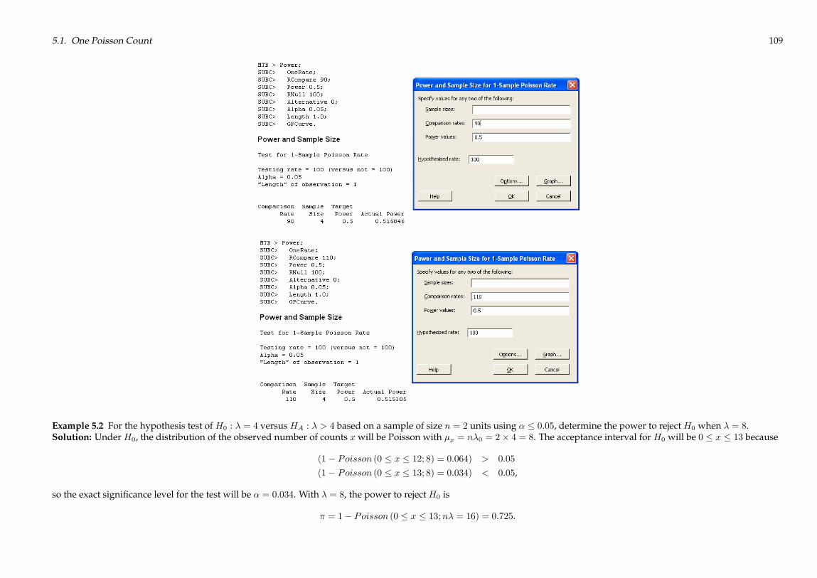
5.1. One Poisson Count 109
Example 5.2 For the hypothesis test of H0 : � = 4 versus HA : � > 4 based on a sample of size n = 2 units using � � 0:05, determine the power to reject H0 when � = 8.Solution: Under H0, the distribution of the observed number of counts xwill be Poisson with �x = n�0 = 2� 4 = 8. The acceptance interval for H0 will be 0 � x � 13 because
(1� Poisson (0 � x � 12; 8) = 0:064) > 0:05
(1� Poisson (0 � x � 13; 8) = 0:034) < 0:05,
so the exact significance level for the test will be � = 0:034. With � = 8, the power to reject H0 is
� = 1� Poisson (0 � x � 13;n� = 16) = 0:725.

110 Chapter 5. Poisson Counts
The count distributions under H0 and HA are shown in Figure 5.1.
From Piface>Generic Poisson test:
MINITAB V16 uses the normal approximation to the Poisson distribution so its answers are different from the exact answers. From MINITAB (V16)> Stat> Power andSample Size> 1-Sample Poisson Rate:

5.1. One Poisson Count 111
Example 5.3 For the hypothesis test of H0 : � = 4 versus HA : � > 4 based on a sample of size n = 5 units, determine the power to reject H0 when � = 9. Use the square roottransformation method with � = 0:05.Solution: By Equation 5.16, the power to reject H0 : � = 4when � = 9 is
� = ���2p5�p9�
p4�+ z0:05 < z <1
�= �(�2:83 < z <1)= 0:9977:
From Piface>Generic Poisson test:

112 Chapter 5. Poisson Counts
From MINITAB (V16)> Stat> Power and Sample Size> 1-Sample Poisson Rate:

5.1. One Poisson Count 113
Example 5.4 How many sampling units must be inspected to reject H0 : � = 10with 90% power in favor of HA : � > 10when in fact � = 15?Solution: By Equation 5.17 the necessary sample size is
n =1
4
�1:645 + 1:282p15�
p10
�2= 4:2,
which rounds up to n = 5 sampling units.
From Piface>Generic Poisson test:

114 Chapter 5. Poisson Counts
From MINITAB (V16)> Stat> Power and Sample Size> 1-Sample Poisson Rate:

5.2. Two Poisson Counts 115
5.2 Two Poisson Counts
Example 5.5 What optimal sample sizes are required to estimate the difference between two Poisson means with 30% precision if the means are expected to be �1 = 25 and�2 = 16?Solution: The difference between the means is expected to be �� = 9, so the confidence interval half-width must be 30% of that, or
� = 0:3� 9 = 2:7.
From Equation 5.24, the optimal sample size ratio isn1n2=
r�1�2=
r25
16= 1:25.
From Equation 5.22, with � = 0:05, the sample size n1 must be
n1 =
�1:96
2:7
�2(25 + 1:25� 16) = 23:7
and the sample size n2 must be
n2 =n1�n1n2
� = 23:7
1:25= 18:96,
which round up to n1 = 24 and n2 = 19.
Example 5.6 How many Poisson counts are required to estimate the ratio of the means of two independent Poisson distributions to within 20% of the true ratio with 95%confidence if the sample sizes will be the same and the ratio of the means is expected to be �1=�2 ' 2?

116 Chapter 5. Poisson Counts
Solution: With n1=n2 = 1, �1=�2 = 2, z0:025 = 1:96, and � = 0:02 in Equation 5.30, the number of Poisson counts required in the first sample is
x1 = (1 + 1� 2)�1:96
0:2
�2= 289.
The corresponding required counts in the second sample are about half of the counts in the first: x2 = 289=2 = 145.
Example 5.7 Determine the power to rejectH0 : �1 = �2 in favor ofHA : �1 < �2 when �1 = 10, n1 = 8 and �2 = 15, n2 = 6. Use the large-sample normal approximation, squareroot transform, and F test methods with � = 0:05.Solution: The expected number of counts from the first (x1) and second (x2) populations are both large enough to justify the large sample approximation method. By thismethod the power is
� = �
0@�1 < z <15� 10q156 +
108
� 1:645
1A= �(�1 < z < 0:937)
= 0:826.
By the log-transformation method the power is
� = �
0@�1 < z <log (15=10)q1
6�15 +1
8�10
� 1:645
1A= �(�1 < z < 0:994)
= 0:840.
By the square-root transform method the power is
� = �
0@�1 < z <
p15�
p10
12
q18 +
16
� 1:645
1A= �(�1 < z < 1:01)
= 0:838.
By the F test method the power is
� = P
�10
15F0:95;2(6)(15);2(8)(10) < F <1
�= P (0:86 < F <1)= 0:837.

5.2. Two Poisson Counts 117
MINITAB V16 supports the two-sample Poisson method but only for equal sample sizes.By the F test method using Piface> Two variances (F Test) with n1 = 2� 6� 15 = 180 and n2 = 2� 8� 10 = 160:
By the F test method using PASS> Variance> Variance: 2 Groups:
Example 5.8 What minimum total counts are required for the two-sample counts test to detect a factor of two difference between the count rates with 90% power? Assume thatthe two sample sizes will be equal.Solution: The hypotheses to be tested are H0 : �1=�2 = 1 versus HA : �1=�2 > 1. From Equation 5.45, which is expressed in terms of the ratio of the two means, the number of

118 Chapter 5. Poisson Counts
count events x1 required to reject H0 when �1=�2 = 2 is
x1 =
�1 +
�1�2
��z� + z�ln (�1=�2)
�2= (1 + 2)
�1:645 + 1:282
ln (2)
�2= 54.
Because �2 = �1=2, the corresponding number of x2 counts is x2 = 54=2 = 27.From MINITAB (V16)> Stat> Power and Sample Size> 2-Sample Poisson Rate:
By trial and error using the F test method in Piface> Two variances (F Test), 90% power is obtained with x1 = 192= (2� 2) = 48 and x2 = 48= (2� 2) = 24:

5.3. Tests for Many Poisson Counts 119
5.3 Tests for Many Poisson Counts
Example 5.9 In a test for differences between mean counts from five different processes, determine the power to reject H0 : �i = �j for all i; j pairs when �1 = �2 = �3 = 16,�4 = 9, �5 = 25 and n = 3 units from each process are inspected. The number of counts will be reported for each unit. Assume that the test will be performed using one-wayANOVA applied to the square root transformed counts.Solution: After the square root transform, the transformed treatment means are �01 = �
02 = �
03 = 4, �
04 = 3, and �05 = 5. The grand transformed mean is �0 = 4, so the treatment
biases relative to the grand mean are 0, 0, 0, �1, and 1, respectively. The ANOVA F test noncentrality parameter is then
� =E(SSTreatment)
E(MS�)=3�02 + 02 + 02 + (�1)2 + (1)2
��12
�2 = 24
where E (MS�) = (�0)2=�12
�2 is the error variance of the transformed counts. The ANOVA will have dfTreatment = 4 and df� = 15� 1� 4 = 10, so the F test critical value willbe F0:95;4;24 = 3:48. The power to reject H0 is then given by Equation 8.1:
F1�� = F1��;�
3:48 = F1��;24
3:48 = F0:11;24,
so the power is � = 0:89 to reject H0 for the specified set of means.
Example 5.10 In a test for differences among the means of five Poisson populations, determine the probability of rejecting H0 : �i = �0 for all i when �i = f16; 16; 16; 12; 20g.The number of units inspected is ni = 4 for all i.Solution: Given the Poisson means specified under HA, the value of �0 under H0 is given by
�0 =1
5(16 + 16 + 16 + 12 + 20) = 16.
With ni = n = 4, the noncentrality parameter is given by
� = nkPi=1
(�A;i � �0)2
�0
= 4
(0)
2
16+(0)
2
16+(0)
2
16+(�4)2
16+(4)
2
16
!= 8.
The power is determined from Equation 5.61:�20:95 = 9:49 = �
20:395;8
where the central and noncentral �2 distributions both have � = 5� 1 = 4 degrees of freedom, so the power is � = 0:605.

120 Chapter 5. Poisson Counts
5.4 Correcting for Background Counts
Example 5.11 In a two-sample test for counts, what common sample size n = n1 = n2 is required to distinguish �1 = �2 = 6 from �1 = 6, �2 = 15 with 90% power in thepresence of a background count rate of �0 = 10?Solution: From Equation 5.55, modified to account for the background count rate, the necessary sample size to reject H0 : �1 = �2 in favor of HA : �1 < �2 with 90% power and� = 0:05 is given by
n =1
2
z� + z��p
�2 + �0 �p�1 + �0
�!2 (5.1)
=1
2
�1:645 + 1:282p25�
p16
�2= 5.
Chapter 6
Regression
6.1 Linear Regression
Example 6.1 Designed experiments frequently involve two or three equally weighted levels of x. Compare the sample sizes required for these two important special cases ifthey must both deliver a �1 confidence interval half-width � and the observations are taken over the same x range from xmin to xmax. For the three-level case, assume that themiddle level will be midway between xmin and xmax.Solution: The subscripts 2 and 3will be used to indicate parameters from the two-level and three-level cases, respectively. For the two-level case, from Equation 6.12 with k2 = 2and�x2 = xmax � xmin, the sample size per x level will be
n2 � 2
�t�=2b����x1
�2� 2
�t�=2b��
� (xmax � xmin)
�2. (6.1)
For the three-level case with k3 = 3 and �x3 = 12 (xmax � xmin) the sample size per x level will be
n3 � 1
2
�t�=2b����x2
�2� 2
�t�=2b��
� (xmax � xmin)
�2. (6.2)
Because n2 = n3, N2 = 2n2, and N3 = 3n2, the two experiments appear to have the same ability to resolve �1 even though the three-level experiment requires 50% moreobservations! This means that the middle observations in the three-level experiment are effectively wasted for the purpose of estimating �1. This statement is not entirely truebecause the middle observations in the three-level experiment do add error degrees of freedom, which potentially decrease n3 compared to n2 for the same �. In general, thepurpose of using three levels of x in an experiment is not to improve the precision of the �1 estimate; rather, three levels are used to allow a linear lack of fit test, which is notpossible using just two levels of x.
121

122 Chapter 6. Regression
Example 6.2 Compare the sample sizes required to estimate the slope parameter with equal precision for two experiments if x is uniformly distributed over the interval fromxmin to xmax in the first experiment and if x has two levels, xmin and xmax, in the second experiment.Solution: From Equations 6.9 and 6.13 the ratio of the total number of observations required by the two experiments is
Nuniform x
Ntwo levels of x'12�
t�=2b���(xmax�xmin)
�24�t�=2b����x
�2where the t�=2 values may differ a bit because of the difference in error degrees of freedom. Both experiments cover the same x range, so�x = xmax � xmin and the sample sizeratio reduces to:
Nuniform x
Ntwo levels of x' 3.
That is, three times as many observations are required in an experiment that uses uniformly distributed x values than if the x values are concentrated at the ends of the xrange. Because we saw in Example 6.1 that the experiment with three evenly spaced, equally weighted levels of x requires 1:5 times as many observations as the two-levelexperiment, other methods of taking evenly spaced, equally weighted observations of x must give experiment sample size ratios between 1:5 and 3. Obviously, the two-levelequally weighted method is the most efficient method for specifying x values for an experiment.
Example 6.3 For an experiment to be analyzed by linear regression with a single predictor, how many observations are required to reject H0 : �1 = 0 in favor of HA : �1 6= 0with 90% power for �1 = 10when a) the distribution of x values will be normal with �x ' 15 and �x ' 2; b) an equal number of observations will be taken at x = 10 and x = 20;c) uniformly distributed values of x will be used over the interval 10 � x � 20; and d) an equal number of observations will be taken at x = 10, 15, and 20. Experience with theprocess tells us the standard error of the model is expected to be �� = 30.Solution:
a) With t ' z in Equation 6.19, the first iteration to find N gives
N = (z0:025 + z0:10)2
�30
10� 2
�2= 24.
Further iterations indicate that the required sample size is N = 26.
From Piface> Linear regression:

6.1. Linear Regression 123
From PASS> Regression> Linear Regression:

124 Chapter 6. Regression
b) The standard deviation of the x values will be
�x =
rSSxN
=
r1
N
N
2
�(�5)2 + (5)2
�= 5.
The first iteration to find N , with t ' z, gives
N = (z0:025 + z0:10)2
�30
10� 5
�2= 4.
Further iterations indicate that N = 7 observations are required.
From Piface> Linear regression:

6.1. Linear Regression 125
c) For uniformly distributed x, the standard deviation of the x values is
�x =xmax � xminp
12=
10p12= 2:89.
With t ' z, the first iteration to find N gives
N = (z0:025 + z0:10)2
�30
10� 2:89
�2= 12.
Further iterations indicate that N = 14 observations are required.From Piface> Linear regression:

126 Chapter 6. Regression
d) The standard deviation of the x values will be
�x =
rSSxN
=
r1
N
N
3
�(�5)2 + (0)2 + (5)2
�= 4:0825.
The first iteration to find N , with t ' z, gives
N = (z0:025 + z0:10)2
�30
10� 4:0825
�2= 6.
Further iterations indicate that N = 9 observations are required.From Piface> Linear regression:
Example 6.4 What is the power to reject H0 for the situation described in Example 6.3a if the sample size is N = 20?Solution: From Equation 6.18 with SSx = N�2x and df� = 20� 2 = 18,
t� =j�1j
pN�x
��� t0:025;18
=10p202
30� 2:10
= 0:881.
The power, as given by Equation 6.17, is
� = P (�1 < t < 0:881)
= 0:805.
From Piface> Linear regression:

6.1. Linear Regression 127
From PASS> Regression> Linear Regression:
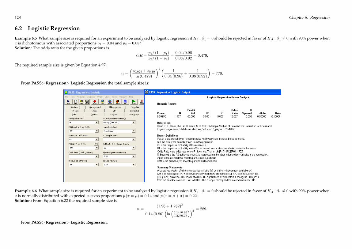
128 Chapter 6. Regression
6.2 Logistic Regression
Example 6.5 What sample size is required for an experiment to be analyzed by logistic regression ifH0 : �1 = 0 should be rejected in favor ofHA : �1 6= 0with 90% power whenx is dichotomous with associated proportions p1 = 0:04 and p2 = 0:08?Solution: The odds ratio for the given proportions is
OR =p1= (1� p1)p2= (1� p2)
=0:04=0:96
0:08=0:92= 0:479.
The required sample size is given by Equation 4.97:
n =
�z0:025 + z0:10ln (0:479)
�2�1
0:04 (0:96)+
1
0:08 (0:92)
�= 770.
From PASS> Regression> Logistic Regression the total sample size is:
Example 6.6 What sample size is required for an experiment to be analyzed by logistic regression ifH0 : �1 = 0 should be rejected in favor ofHA : �1 6= 0with 90% power whenx is normally distributed with expected success proportions p (x = �) = 0:14 and p (x = �+ �) = 0:22.Solution: From Equation 6.22 the required sample size is
n =(1:96 + 1:282)
2
0:14 (0:86)�ln�0:14=0:860:22=0:78
��2 = 289.
From PASS> Regression> Logistic Regression:

6.2. Logistic Regression 129

130 Chapter 6. Regression

Chapter 7
Correlation and Agreement
7.1 Pearson’s Correlation
Example 7.1 Determine the number of paired observations required to obtain the following confidence interval for the population correlation:
P (0:9 < � < 0:99) = 0:95.
Solution: The Fisher’s Z-transformed confidence interval is
P (Z0:9 < Z� < Z0:99) = 0:95
P (1:472 < Z� < 2:647) = 0:95.
Then with � = 0:05 in Equation 7.10, the required sample size is
n = 4
�1:96
2:647� 1:472
�2+ 3
= 15.
Example 7.2 An experiment is planned to test H0 : � = 0:9 versus HA : � < 0:9 on the basis of n = 28 paired observations. Determine the power of the test to reject H0 when� = 0:7.Solution: Under H0 following Fisher’s transform we have
(�Z)0 =1
2ln
�1 + 0:9
1� 0:9
�= 1:472
and by Equation 7.4
�Z =1p28� 3
= 0:2.
131

132 Chapter 7. Correlation and Agreement
For the one-sided left-tailed test, the critical value of Z that distinguishes the accept/reject regions is given by
ZA=R = (�Z)0 � z��z= 1:472� z0:05 (0:2)= 1:472� 1:645 (0:2)= 1:143.
The corresponding Z value under HA when � = 0:7 is
(�Z)A =1
2ln
�1 + 0:7
1� 0:7
�= 0:867.
Then the power to reject H0 when � = 0:7 is
� = ���1 < Z < ZA=R; (�Z)A ; �Z
�= �(�1 < Z < 1:143; 0:867; 0:2)
= � (�1 < z < 1:38)
= 0:916.
From PASS> Correlations> Correlations: One:
Example 7.3 Find the power to reject H0 : �1 = �2 in favor of HA : �1 6= �2 when �1 = 0:99, �2 = 0:95, and n1 = n2 = 30.

7.1. Pearson’s Correlation 133
Solution: The Fisher-transformed difference between the two correlations under HA is
�Z = Z1 � Z2
=1
2ln
�1 + 0:99
1� 0:99
�� 12ln
�1 + 0:95
1� 0:95
�= 0:815.
From Equations 7.11 and 7.14 with � = 0:05 the power is
� = �
0@�1 < z <
0@ 0:815q2
30�3
� 1:96
1A1A= �(�1 < z < 1:03)
= 0:85.
From PASS> Correlations> Correlations: Two:
Example 7.4 What sample size should be drawn from two populations to perform the two-sample test for correlation (H0 : �1 = �2 versus HA : �1 6= �2) with 90% power toreject H0 when �1 = 0:9 and �2 = 0:8?

134 Chapter 7. Correlation and Agreement
Solution: The Fisher-transformed difference between the two correlations is
�Z = Z1 � Z2
=1
2ln
�1 + 0:9
1� 0:9
�� 12ln
�1 + 0:8
1� 0:8
�= 0:374.
From Equation 7.15 with � = 0:05 and � = 0:10 the required common sample size is
n = 2
�1:96 + 1:28
0:374
�2+ 3
= 154.
From PASS> Correlations> Correlations: Two:
Example 7.5 Determine the power to reject H0 : �2 = 0when in fact �2 = 0:6 based on a sample of n = 20 observations taken with four random covariates.Solution: The regression model for y as a function of the four predictors will have dfmodel = k = 4model degrees of freedom and df� = n� k� 1 = 20� 4� 1 = 15 error degreesof freedom. The F distribution noncentrality parameter from Equation 7.19 with �2 = 0:6 is
� = 200:6
1� 0:6 = 30.
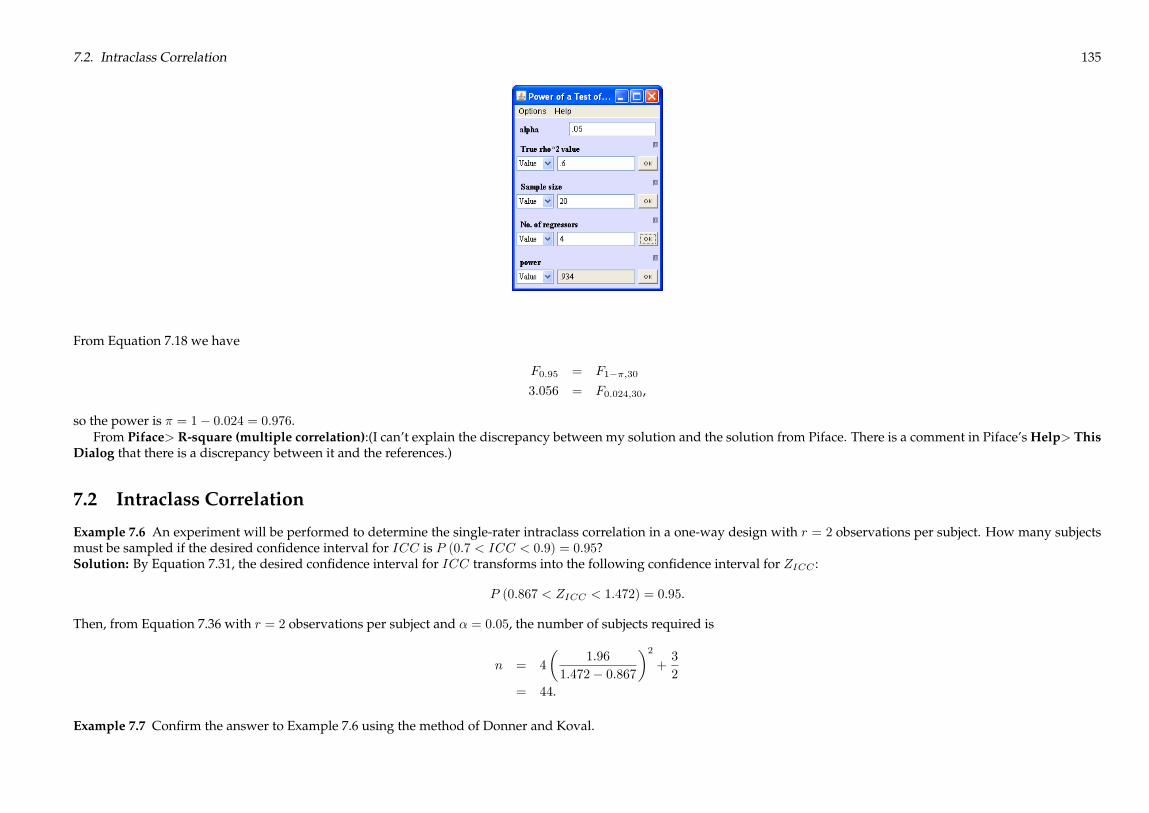
7.2. Intraclass Correlation 135
From Equation 7.18 we have
F0:95 = F1��;30
3:056 = F0:024;30,
so the power is � = 1� 0:024 = 0:976.From Piface> R-square (multiple correlation):(I can’t explain the discrepancy between my solution and the solution from Piface. There is a comment in Piface’s Help> This
Dialog that there is a discrepancy between it and the references.)
7.2 Intraclass Correlation
Example 7.6 An experiment will be performed to determine the single-rater intraclass correlation in a one-way design with r = 2 observations per subject. How many subjectsmust be sampled if the desired confidence interval for ICC is P (0:7 < ICC < 0:9) = 0:95?Solution: By Equation 7.31, the desired confidence interval for ICC transforms into the following confidence interval for ZICC :
P (0:867 < ZICC < 1:472) = 0:95.
Then, from Equation 7.36 with r = 2 observations per subject and � = 0:05, the number of subjects required is
n = 4
�1:96
1:472� 0:867
�2+3
2
= 44.
Example 7.7 Confirm the answer to Example 7.6 using the method of Donner and Koval.

136 Chapter 7. Correlation and Agreement
Solution: Assuming that [ICC = 0:8, the sample size according to Donner and Koval is given by Equation 7.38:
n =8
2 (2� 1)
�1:96 (1� 0:8) (1 + (2� 1) 0:8)
0:9� 0:7
�2= 50,
which is in reasonable agreement with the sample size determined by the Fisher’s transformation method.
Example 7.8 How many subjects are required in an experiment to reject H0 : ICC = 0:6 with 80% power when ICC = 0:8 and two raters will rate each subject? Confirm thesample size by calculating the exact power.Solution: From Equation 7.31 the ZICC values corresponding to ICC = 0:6 and ICC = 0:8 are Z0 = 0:693 and Z1 = 1:099, respectively. From Equation 7.42 with r = 2 and� = 0:05, the approximate sample size is
n =
�z0:05 + z0:20Z1 � Z0
�2+3
2
=
�1:645 + 0:84
1:099� 0:693
�2+3
2
= 39.
The exact power is given by Equation 7.39 where the F distribution has df1 = 39 � 1 = 38 numerator degrees of freedom and df2 = 39 (2� 1) = 39 denominator degrees offreedom. The power is given by
� = P
0@1 + 2�
0:61�0:6
�1 + 2
�0:81�0:8
�F0:95 < F <11A
= P (0:760 < F <1)= 0:80,
which is in excellent agreement with the target power.
From PASS> Correlation> Intraclass Correlation:

7.3. Cohen’s Kappa 137
7.3 Cohen’s Kappa
Example 7.9 How many units should two operators evaluate in an attribute inspection agreement experiment to be analyzed using Cohen’s � if the true value of the unknown� must be determined to within �0.10 with 95% confidence? A preliminary experiment indicated that � ' 0:85 and pe ' 0:5.Solution: With � = 0:05 and � = 0:10 in Equation 7.55, the required sample size is
n =0:85 (1� 0:85)
1� 0:5
�1:96
0:10
�2= 98.
Example 7.10 Calculate the power to reject H0 : � = 0:4 in favor of HA : � > 0:4when � = 0:7 if a sample of size n = 70 is allocated to k = 3 categories in the ratio 0:4 : 0:5 : 0:1.Solution: The expected chance agreement by Equation 7.46 is pe = 0:42 + 0:52 + 0:12 = 0:42. The two � values of interest have intermediate values not covered by the large- orsmall-� approximations, so it is necessary to estimate �b� using Equation 7.47. Under H0 with � = 0:4 and pe = 0:42 in Equation 7.44, we have
po = 0:4 (1� 0:42) + 0:42= 0:652,
so
�b�0 ' 1
1� 0:42
r0:652 (1� 0:652)
70' 0:0982.

138 Chapter 7. Correlation and Agreement
Under HA with � = 0:7we have
po = 0:7 (1� 0:42) + 0:42= 0:826,
so
�b�1 ' 1
1� 0:42
r0:826 (1� 0:826)
70' 0:0781.
Then with � = 0:05, z� is given by Equation 7.58:
z� =(0:7� 0:4)� 1:645 (0:0982)
0:0781= 1:77
and the power is given by Equation 7.57:
� = �(�1 < z < 1:77)
= 0:962.
Example 7.11 An experiment is to be performed to test for agreement between two methods of categorizing a dichotomous response. The hypotheses to be tested areH0 : � = 0versus HA : � > 0 where � is Cohen’s kappa. How many units must be inspected if the test should have 90% power to reject H0 when � = 0:40 and the total number of units tobe inspected is evenly split between the two categories?Solution: Because the units will be balanced between the two categories, the agreement expected by chance from Equation 7.51 is pe ' 0:5. With � = 0:05, � = 0:90,� = 1� � = 0:10, and � = 0:4� 0 = 0:4 in Equation 7.59, the required sample size is
n ' 0:5
1� 0:5
�z0:05 + z0:10
�
�2=
�1:645 + 1:282
0:40
�2= 54.
Example 7.12 An experiment is to be performed to test for agreement between two raters using a categorical four-state response. The hypotheses to be tested are H0 : � = 0:8versus HA : � > 0:8. How many units must be inspected if the test should have 90% power to reject H0 when � = 0:9? The units to be inspected are evenly balanced across thefour categories.Solution: From Equation 7.51 with k = 4 categories, pe ' 0:25. With � = 0:05, � = 1� � = 0:10, and � = 0:9� 0:8 = 0:1 in Equation 7.60, the required sample size is
n ' 1
1� 0:25
�1:645
p0:8� 0:2 + 1:282
p0:9� 0:1
0:9� 0:8
�2' 145.

7.4. Receiver Operating Characteristic (ROC) Curves 139
7.4 Receiver Operating Characteristic (ROC) Curves
Example 7.13 What sample size is required to estimate the value of an ROC curve’s AUC to within �0.05 with 95% confidence if the AUC value is expected to be about 90%?Solution: The desired confidence interval has the form
P�[AUC � 0:05 < AUC < [AUC + 0:05
�= 0:95.
With � = 0:05, AUC = 0:90, and � = 0:05 in Equation 7.66, the required sample size is
n ' 1�AUC2
�z0:025�
�2' 1� 0:90
2
�1:96
0:05
�2' 77.
That is, about 77 positives and 77 negatives are required. The large-sample and large AUC assumptions are reasonably satisfied, so this approximate sample size should beaccurate.
From PASS>Diagnostic Tests> ROC Curve - 1 Test:

140 Chapter 7. Correlation and Agreement
Example 7.14 What sample size is required to reject H0 : AUC = 0:9 in favor of HA : AUC 6= 0:9with 90% power when AUC = 0:95?Solution: With � = 0:05 in Equation 7.67, the required sample size is approximately
n =
0@q
1�0:902 z0:025 +
q1�0:952 z0:10
0:95� 0:90
1A2
=
0@q
1�0:902 1:96 +
q1�0:952 1:282
0:95� 0:90
1A2
= 165.
From PASS>Diagnostic Tests> ROC Curve - 1 Test:
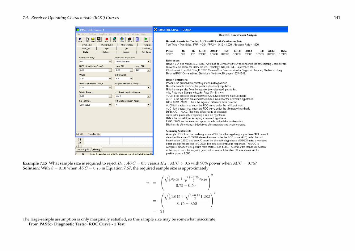
7.4. Receiver Operating Characteristic (ROC) Curves 141
Example 7.15 What sample size is required to reject H0 : AUC = 0:5 versus HA : AUC > 0:5with 90% power when AUC = 0:75?Solution: With � = 0:10when AUC = 0:75 in Equation 7.67, the required sample size is approximately
n =
0@q
16z0:05 +
q1�0:752 z0:10
0:75� 0:50
1A2
=
0@q
161:645 +
q1�0:752 1:282
0:75� 0:50
1A2
= 21.
The large-sample assumption is only marginally satisfied, so this sample size may be somewhat inaccurate.From PASS>Diagnostic Tests> ROC Curve - 1 Test:

142 Chapter 7. Correlation and Agreement
7.5 Bland-Altman Plots
Example 7.16 What minimum sample size is required to demonstrate the agreement between two methods to measure length by the Bland-Altman method if the limits ofagreement are LOAU=L = �3cm and the standard deviation of the differences had been estimated to be b�d = 0:65cm from historical data? Assume that the limits of agreementmust cover 99% of the samples with 95% confidence and that there is no bias between the two methods, i.e., �d = 0.Solution: The two-sided normal distribution tolerance interval factor k2 is given by
k2 =LOAb�d
=3cm
0:65cm= 4:615.

7.5. Bland-Altman Plots 143
With � = 0:05 and Y = 0:99 in Appendix E, Table E.7, the smallest sample size that gives k2 � 4:615 is n = 10.

144 Chapter 7. Correlation and Agreement

Chapter 8
Designed Experiments
8.1 One-Way Fixed Effects ANOVA
Example 8.1 In a one-way classification design with four treatments and five observations per treatment, determine the power of the ANOVA to rejectH0 if the treatment meansare �i = f40; 55; 55; 50g. The four populations are expected to be normal and homoscedastic with �� = 8.Solution: The grand mean is �� = 50 so the treatment biases relative to the grand mean are � i = f�10; 5; 5; 0g. From Equation 8.2 the F distribution noncentrality parameter is,
� =
nkPi=1
�2i
�2�=5��102 + (5)2 + (5)2 + (0)2
�82
= 11:72.
The F statistic will have dftreatments = 4� 1 = 3 and df� = 4 (5� 1) = 16 degrees of freedom. The power is 72% as determined from Equation 8.1:
F0:95 = 3:239 = F0:280;11:72.
From Piface> Balanced ANOVA (any model)>One-way ANOVA with:
sA =
vuut�(�10)2 + (5)2 + (5)2 + (0)2�4� 1 = 7:07
145

146 Chapter 8. Designed Experiments
From PASS>Means>Many Means> ANOVA: One-Way:

8.1. One-Way Fixed Effects ANOVA 147
MINITAB> Stat> Power and Sample Size> One-Way ANOVA cannot be used to solve this problem because it does not allow specification of the individual treatmentmeans or the standard deviation of the treatment means. The steps required to calculate the power from the model and error degress of freedom and the noncentrality parameterusing MINITAB> Calc> Probability Distributions> F are:
MTB invcdf 0.95;SUBC f 3 16.
F distribution with 3 DF in numerator and 16 DF in denominator
P(~X~=~x~) x0.95 3.23887
MTB cdf 3.23887;SUBC f 3 16 11.72.
F distribution with 3 DF in numerator and 16 DF in denominator and noncentrality parameter 11.72
x P(~X~=~x~)3.23887 0.279568
Power = 1 - 0.280 = 0.720
Example 8.2 Determine the power of the ANOVA to rejectH0 in a one-way classification design with four treatments and five observations per treatment if the treatment biasesfrom the grand mean are � i = f�12; 12; 0; 0g. The four populations are expected to be normal and homoscedastic with �� = 8.
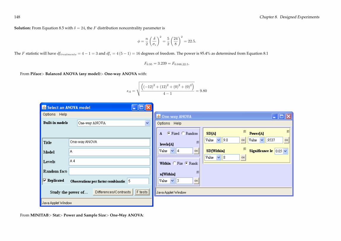
148 Chapter 8. Designed Experiments
Solution: From Equation 8.5 with � = 24, the F distribution noncentrality parameter is
� =n
2
��
��
�2=5
2
�24
8
�2= 22:5.
The F statistic will have dftreatments = 4� 1 = 3 and df� = 4 (5� 1) = 16 degrees of freedom. The power is 95.4% as determined from Equation 8.1
F0:95 = 3:239 = F0:046;22:5.
From Piface> Balanced ANOVA (any model)>One-way ANOVA with:
sA =
vuut�(�12)2 + (12)2 + (0)2 + (0)2�4� 1 = 9:80
From MINITAB> Stat> Power and Sample Size>One-Way ANOVA:

8.1. One-Way Fixed Effects ANOVA 149
From PASS>Means>Many Means> ANOVA: One-Way:
Example 8.3 In a one-way classification design with four treatments and five observations per treatment, determine the power of the ANOVA to rejectH0 if the treatment biasesfrom the grand mean are � i = f18;�6;�6;�6g. The four populations are expected to be normal and homoscedastic with �� = 8.

150 Chapter 8. Designed Experiments
Solution: From Equation 8.6 with � = 24, the F distribution noncentrality parameter is
� =n (k � 1)
k
��
��
�2=5� 34
�24
8
�2= 33:75.
The F statistic will have dftreatments = 4� 1 = 3 and df� = 4 (5� 1) = 16 degrees of freedom. The power is 99.5% as determined from Equation 8.1:
F0:95 = 3:239 = F0:005;33:75.
From Piface> Balanced ANOVA (any model)>One-way ANOVA with:
sA =
vuut�(18)2 + (�6)2 + (�6)2 + (�6)2�4� 1 = 12:0
From PASS>Means>Many Means> ANOVA: One-Way:

8.1. One-Way Fixed Effects ANOVA 151
Example 8.4 Determine the power to reject H0 by one-way ANOVA when the treatment means are �i = f50; 30; 40; 40; 40g and the sample sizes are ni = f12; 12; 20; 20; 15g. Thefive populations are expected to be normal and homoscedastic with �� = 13.Solution: The grand mean of the experimental data is expected to beP
ni�iPni
=(50� 12) + � � �+ (40� 15)
12 + � � �+ 15 = 40.
The treatment biases relative to the grand mean are � i = f10;�10; 0; 0; 0g so the noncentrality parameter is
� =12 (10)
2+ 12 (�10)2 + 20 (0)2 + 20 (0)2 + 15 (0)2
132= 14:2.
The ANOVA will have dftreatments = 5� 1 = 4 and df� =Pni � 1� 4 = 74 degrees of freedom. The power is 84.7% as determined from Equation 8.1:
F0:95 = 2:495 = F0:153;14:2.

152 Chapter 8. Designed Experiments
8.2 Randomized Block Design
Example 8.5 Recalculate the power for Example 8.1 if the experiment is built as a randomized block design and the standard deviation of the population of block biases is�blocks = 4.Solution: The F distribution noncentrality parameter (� = 11:72) and the treatment degrees of freedom (dftreatments = 3) will be unchanged from the original solution, but ifthe experiment is built in five blocks with one replicate in each block, the new error degrees of freedom for the RBD will be
df� = dftotal � dftreatments � dfblocks= 19� 3� 4= 12.
The power of the RBD is 68% as determined fromF0:95 = 3:490 = F0:32;11:72.
This is slightly lower than the original power (72%) because the RBD has fewer error degrees of freedom than the CRD. The RBD’s power is not affected by the block variationbecause it separates that variation from the error variation that is used to determine the power.
From Piface> Balanced ANOVA (any model)> Two-way ANOVA (additive model) with:

8.3. Balanced Full Factorial Design with Fixed Effects 153
From PASS>Means>Many Means> ANOVA: Fixed Effect:
Example 8.6 A 40-run experiment was performed using an RBD with k = 5 treatments and r = 8 blocks. The ANOVA table from the experiment is shown in Table 8.2. Calculatethe blocking efficiency and the increase in the number of runs required to obtain the same estimation precision for treatment means using a CRD.Solution: The blocking efficiency as determined from Equation 8.13 is
E =(7� 14) + (8� 4� 4)
(5� 8� 1) 4= 1:45.
That is, the CRD will require about 45% more runs than the RBD because it ignores the variation associated with block effects. Because the number of runs in the RBD waskr = 40, the number of runs required for the CRD to obtain the same estimation precision for the treatment means would be Ekr = 1:45� 40 = 58. Apparently the blocking wasbeneficial and should be used in future studies.
8.3 Balanced Full Factorial Design with Fixed Effects
Example 8.7 A 2� 3� 5 full factorial experiment with four replicates is planned. The experiment will be blocked on replicates and the ANOVA model will include main effectsand two-factor interactions. Determine the power to detect a difference � = 300 units between two levels of each study variable if the standard error of the model is expected to

154 Chapter 8. Designed Experiments
be �� = 500.Solution: If the three study variables are given the names A, B, and C and have a = 2, b = 3, and c = 5 levels, respectively, then the degrees of freedom associated with the termsin the model will be dfblocks = 3, dfA = 1, dfB = 2, dfC = 4, dfAB = 2, dfAC = 4, dfBC = 8, and
df� = dftotal � dfmodel= (2� 3� 5� 4� 1)� (3 + 1 + 2 + 4 + 2 + 4 + 8)= 119� 24= 95.
From Equation 8.2, the F distribution noncentrality parameter for variable Awith treatment biases �1 = �150 and �2 = 150 is
�A =
bcn2Pi=1
�2i
�2�
=3� 5� 4�
�(�150)2 + 1502
�5002
= 10:8.
The distribution of FA will have dfA = 1 numerator and df� = 95 denominator degrees of freedom, so the power associated with A is given by Equation 8.1:
F0:95 = 3:942 = F1��A;10:8,
which is satisfied by �A = 0:908 or 90.8%.Similarly, the F distribution noncentrality parameter for B with biases
�1 = �150, �2 = 150, and �3 = 0 is
�B =
acn3Pi=1
�2i
�2�
=2� 5� 4�
�(�150)2 + 1502 + 02
�5002
= 7:2.
The distribution of FB will have dfB = 2 numerator and df� = 95 denominator degrees of freedom, so the power associated with B is given by
F0:95 = 3:093 = F1��B ;7:2,
which is satisfied by �B = 0:654.
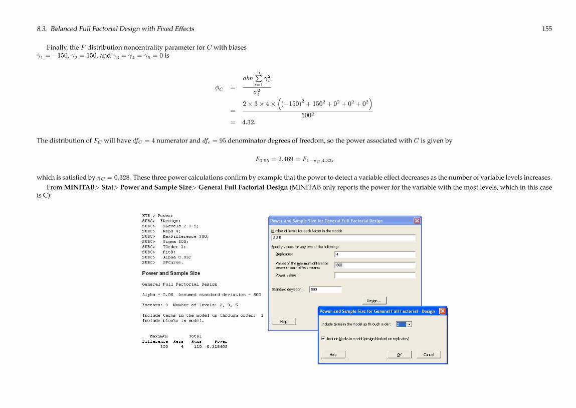
8.3. Balanced Full Factorial Design with Fixed Effects 155
Finally, the F distribution noncentrality parameter for C with biases 1 = �150, 2 = 150, and 3 = 4 = 5 = 0 is
�C =
abn5Pi=1
2i
�2�
=2� 3� 4�
�(�150)2 + 1502 + 02 + 02 + 02
�5002
= 4:32.
The distribution of FC will have dfC = 4 numerator and df� = 95 denominator degrees of freedom, so the power associated with C is given by
F0:95 = 2:469 = F1��C ;4:32,
which is satisfied by �C = 0:328. These three power calculations confirm by example that the power to detect a variable effect decreases as the number of variable levels increases.From MINITAB> Stat> Power and Sample Size>General Full Factorial Design (MINITAB only reports the power for the variable with the most levels, which in this case
is C):

156 Chapter 8. Designed Experiments
From Piface> Balanced ANOVA (any model)> Three-way ANOVA with
sA =
r�2 (150)
2�= (2� 1) = 212:1
sB =
r�2 (150)
2+ (0)
2�= (3� 1) = 150:0
sC =
r�2 (150)
2+ 3 (0)
2�= (5� 1) = 106:1

8.3. Balanced Full Factorial Design with Fixed Effects 157
From PASS>Means>Many Means> ANOVA: Fixed Effect:

158 Chapter 8. Designed Experiments
MINITAB doesn’t have a built in capability to do sample size and power calculations for multi-way ANOVA, however, the custom macro power.mac (posted at www.mmbstatistical.com/SampleSize/)can be used to calculate the power for one design variable at a time in a balanced multi-way ANOVA. For the first variable:
MTB %power c1Executing from file: C:\Program Files\Minitab 15\English\Macros\power.MAC
Do you want to specify your design from the terminal or from a column?
If from terminal a column will be created in the column specified.Otherwise the column specified will be the input.
(terminal=1, column=2)DATA 1
How many runs are in one replicate?DATA 30
How many replicates?DATA 4
How many levels does the variable have?DATA 2

8.4. Random and Mixed Models 159
How many model degrees of freedom are there?DATA 24
What is the standard deviation?DATA 500
What is the smallest difference that youwant to detect between two levels?DATA 300
N 120.000Runs 30.0000reps 4.00000Levels 2.00000dfmodel 24.0000dferror 95.0000Fcrit 3.94122lambda 10.8000sigma 500.000delta 300.000Power 0.901990
8.4 Random and Mixed Models
Piface can calculate sample size and power for random and mixed models but MINITAB and PASS can not.
Example 8.8 A balanced full factorial experiment is to be performed using a = 3 levels of a fixed variable A, b = 5 randomly selected levels of a random variable B, and n = 4replicates. Determine the power to reject H0 : �i = 0 for all i when the A-level biases are �i = f�20; 20; 0g with �B = 25, �AB = 0, and �� = 40. Assume that the AB interactionterm will be included in the ANOVA even though its expected variance component is 0.Solution: The ANOVA table with the equations for the expected mean squares is shown in Table 8.3. From the ANOVA table, the error mean square used for testing the A effect(that is, the denominator of FA) is
MS�(A) = MSAB
= b�2� + nb�2AB .
The noncentrality parameter for the test of the fixed effect A is given by Equation 8.15:
�A =N
a
Xa
i=1�2i
MS�(A)
=3� 5� 4
3
(�20)2 + (20)2 + (0)2
(40)2+ 4 (0)
2
= 10.

160 Chapter 8. Designed Experiments
With dfA = 2, dfAB = 8, and � = 0:05 in Equation 8.1
F0:95 = 4:459 = F1��;10:0,
which is satisfied by � = 0:640.From Piface> Balanced ANOVA (any model) with:
sA =
r�(�20)2 + (20)2 + (0)2
�= (3� 1) = 20
Example 8.9 Determine the power to reject H0 : �2B = 0 when �B = 25, �AB = 0, and �� = 40 for Example 8.8. Retain the AB interaction term in the model even though itsvariance component is 0.Solution: The ANOVA table with the equations for the expected mean squares is shown in Table 8.3. From Equation 8.19 under the specified conditions, the expected FB value

8.5. Nested Designs 161
is approximately
E (FB) ' E (MSB)
E (MSAB)
' �2� + n�2AB + an�
2B
�2� + n�2AB
' (40)2+ 4 (0)
2+ 3� 4� (25)2
(40)2+ 4 (0)
2
' 5:69.
With dfB = 4, dfAB = 8, and � = 0:05, the critical F value for the test for the B effect is F0:95;4;8 = 3:838, so from Equation 8.20 the power is approximately
� ' P
�3:838
5:69< F <1
�' P (0:675 < F <1)' 0:618.
See Piface solution to Example 8.8.
8.5 Nested Designs
Example 8.10 A is a fixed variable with three levels and B is a random variable with four levels nested within each level of A. The nested design is crossed with a five-level fixedvariable C and one replicate of the experiment will be built. The model to be fitted is: A+B (A)+C +AC +BC. Find the power to detect a difference � = 40 between two levelsof A assuming that the standard deviations for the random effects are �B = 12, �BC = 4, and �� = 10.Solution: The ANOVA table with the equations for the expected mean squares is shown in Table 8.4 where the �i are the A-level biases, the � i are the C-level biases, and the iare the AC interaction biases. The error mean square used for testing the A effect is MS�(A) = MSB(A). The noncentrality parameter for the test of the fixed effect A is given byEquation 8.15:
�A =a� b� c� n
a
Xa
i=1�2i
�2� + n�2BC + cn�
2B(A)
=3� 4� 5� 1
3
(�20)2 + (20)2 + (0)2
(10)2+ (4)
2+ 5 (12)
2
= 19:14.
With dfA = 2, dfB(A) = 3 (4� 1) = 9, and � = 0:05 in Equation 8.1:F0:95 = 4:256 = F1��;19:14
which is satisfied by � = 0:915.

162 Chapter 8. Designed Experiments
From Piface> Balanced ANOVA (any model) with:
sA =
s2 (20)
2+ (0)
2
3� 1 = 20:0
8.6 Two-Level Factorial Designs
Example 8.11 Use the method of Equation 8.24 to determine the number of replicates required to detect an effect of size � = 6with 90% power in a 24 experiment when �� = 10.Assume that the ANOVA model will include main effects and two-factor interactions.Solution: With t ' z in the first iteration of Equation 8.24, the number of replicates required to deliver 90% power to detect the difference � = 6 between two levels of a designvariable is
n � 1
24�2(1:96 + 1:282)
2
�10
6
�2� 8.
Another iteration (not shown) confirms that n = 8 is the correct number of replicates.See Example 8.12.
Example 8.12 Use the method of Equation 8.21 to confirm the solution to Example 8.11.Solution: By Equation 8.22 the F distribution noncentrality parameter is
� = 8� 24�2�6
10
�2= 11:5.
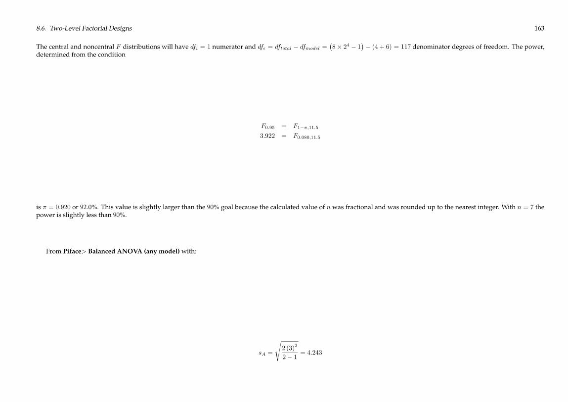
8.6. Two-Level Factorial Designs 163
The central and noncentral F distributions will have dfi = 1 numerator and df� = dftotal � dfmodel =�8� 24 � 1
�� (4 + 6) = 117 denominator degrees of freedom. The power,
determined from the condition
F0:95 = F1��;11:5
3:922 = F0:080;11:5
is � = 0:920 or 92.0%. This value is slightly larger than the 90% goal because the calculated value of n was fractional and was rounded up to the nearest integer. With n = 7 thepower is slightly less than 90%.
From Piface> Balanced ANOVA (any model) with:
sA =
s2 (3)
2
2� 1 = 4:243

164 Chapter 8. Designed Experiments
From MINITAB> Stat> Power and Sample Size> 2-Level Factorial Design (with 5 terms removed from the model: four three-factor interactions and the one four-factorinteraction):

8.6. Two-Level Factorial Designs 165
Example 8.13 Suppose that two more two-level variables were added to the 24 experiment with n = 8 replicates from Example 8.11 without any increase in the total number ofruns. Calculate the power for the resulting 26 experiment.Solution: The 26 experiment must have n = 2 replicates to maintain the same number of runs as the original experiment. Because 8�24 = 2�26, the F distribution noncentralityparameter will be unchanged. The new error degrees of freedom for the F distributions will be df� =
�2� 26 � 1
�� (6 + 15) = 106. The power, determined from
F0:95 = F1��;11:5
3:931 = F0:081;11:5
is � = 0:919 or 91.9%. This example confirms that adding variables to a 2k design without increasing the total number of observations has little effect on the power provided thatthe error degrees of freedom remains large.
From Piface> Balanced ANOVA (any model):
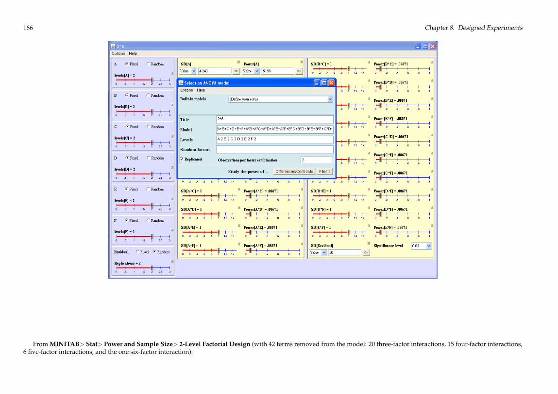
166 Chapter 8. Designed Experiments
From MINITAB> Stat> Power and Sample Size> 2-Level Factorial Design (with 42 terms removed from the model: 20 three-factor interactions, 15 four-factor interactions,6 five-factor interactions, and the one six-factor interaction):

8.6. Two-Level Factorial Designs 167
Example 8.14 Derive a simplified expression for the total number of observations required for a 2k experiment to detect a difference � between two levels of a design variableassuming � = 0:05 and � = 0:10. Under what conditions should this expression be valid?Solution: From Equation 8.25 the total number of replicates required for a 2k design to have 90% power to detect a difference � between two levels of a design variable isapproximately
n2k � 4 (z0:025 + z0:10)2����
�2� 42
����
�2. (8.1)
This condition will be strictly valid when df� is large so that the t ' z approximation is well satisfied.
Example 8.15 How many replicates of a 23 design are required to determine the regression coefficient for a main effect with precision � = 300 with 95% confidence when thestandard error of the model is expected to be �� = 600?Solution: If the error degrees of freedom are sufficiently large that t0:025 ' z0:025 then
n � 1
23
�1:96� 600300
�2� 2.

168 Chapter 8. Designed Experiments
With only 2 � 23 = 16 total runs, the t0:025 ' z0:025 assumption is not satisfied. Another iteration shows that the transcendental sample size condition is satisfied for n = 3replicates of the 23 design.
Example 8.16 What is the power for the 24�1IV design with two replicates to detect a difference of � = 10 between two levels of a design variable if �� = 5?Solution: With two replicates the total number of experimental runs will be 2
�24�1
�= 16. Because the experiment design is resolution IV, the model can include main effects and
only three of the six possible two-factor interactions, so dfmodel = 4 + 3 = 7. Then, the error degrees of freedom will be df� = (16� 1) � 7 = 8. The F distribution noncentralityparameter associated with a difference of � = 10 between two levels of a design variable is given by a slightly modified form of Equation 8.22:
� = n2(k�p)�2��
��
�2(8.2)
= 2� 2(4�1)�2�10
5
�2= 16:0
where p = 1 accounts for the half-fractionation of the full factorial design. Then, by Equation 8.21
F0:95 = F1��;16
5:318 = F0:063;16.
The power is � = 1� 0:063 = 0:937.From MINITAB> Stat> Power and Sample Size> 2-Level Factorial Design:

8.6. Two-Level Factorial Designs 169
Example 8.17 How many replicates of a 25�1V design are required to have 90% power to detect a difference � = 0:4 between two levels of a design variable? Assume that ten ofthe fifteen possible terms will drop out of the model and that the standard error will be �� = 0:18.Solution: If a model with main effects and two factor interactions is fitted to one replicate of the 25�1V design, there will not be any degrees of freedom left to estimate the error,so either the experiment must be replicated or some terms must be dropped from the model. Under the assumption that the number of replicates is large, so that we can taket ' z in the first iteration of Equation 8.24, we have
n � 1
2(5�1)�2(z0:025 + z0:10)
2
�0:18
0:4
�2� 0:532.
Obviously, the t ' z approximation is not satisfied, so at least one more iteration is required. If only one replicate of the half-fractional factorial design is built and ten of thefifteen possible terms are dropped from the model, the error degrees of freedom will be df� = 15� 10 = 5. Then, for the second iteration of Equation 8.24, we have
n � 1
2(5�1)�2(t0:025 + t0:10)
2
�0:18
0:4
�2� 1
2(5�1)�2(2:228 + 1:372)
2
�0:18
0:4
�2� 0:656,
which rounds up to n = 1. Calculation of the power (not shown) confirms � = 0:98 for one replicate.
From MINITAB> Stat> Power and Sample Size> 2-Level Factorial Design:

170 Chapter 8. Designed Experiments
Example 8.18 How many replicates of a 9-variable 12-run Plackett-Burman design are required to detect a difference � = 7000 between two levels of a variable with 90% powerif the standard error is expected to be �� = 4000?Solution: Plackett-Burman designs are resolution III, so their models may contain only main effects. If the experiment is run with only one replicate, then df� = (12� 1)� 9 = 2and the large-sample approximation is obviously not satisfied. If enough replicates are run so that the large-sample approximation is satisfied, then with � = 0:05, � = 0:10 andt ' z, the approximate number of replicates required is
n � 4
12(1:96 + 1:282)
2
�4000
7000
�2� 2.
Another iteration confirms that two replicates are sufficient to achieve 90% power.
From MINITAB> Stat> Power and Sample Size> Plackett-Burman Design:

8.7. Two-Level Factorial Designs with Centers 171
8.7 Two-Level Factorial Designs with Centers
Example 8.19 Calculate the power to detect a difference � = 1400 between two levels of a study variable in a 23 design with three replicates built in blocks with two center pointsper block. Include terms for main effects, two-factor interactions, lack of fit, and blocks in the model. The standard error is expected to be �� = 1000.Solution: The experiment will have 3
�23 + 2
�= 30 total observations, so the total degrees of freedom will be dftotal = 29. The degrees of freedom for the model will be
dfmodel = dfblocks + dfmain effects + dfinteractions + dfLOF
= 2 + 3 + 3 + 1
= 9,
so the error degrees of freedom will bedf� = dftotal � dfmodel = 29� 9 = 20.
The power � to reject H0 : � = 0 for the main effect of any one of the study variables is given by Equation 8.21 with one numerator and twenty denominator degrees of freedomwhere the F distribution noncentrality parameter, as given in Equation 8.22, is
� = 3� 23�2�1400
1000
�2= 11:76.
With � = 0:05 and
F1�� = F1��;�
F0:95 = 4:351 = F1��;8:17,

172 Chapter 8. Designed Experiments
we find the power to be � = 0:903.From MINITAB> Stat> Power and Sample Size> 2-Level Factorial Design:
Example 8.20 Determine the ratio of the precisions of the estimates for the lack of fit and main effects in a 24 plus centers design when two center points are used per replicate.Solution: From Equation 8.39 with k = 4 and n0 = 2 the ratio of the lack of fit and main effect precision estimates will be
����
=
r1 +
24
2= 3.
That is, the confidence interval for the lack of fit estimate will be three times wider than the confidence interval for the main effects.
8.8 Response Surface Designs
Example 8.21 How many replicates of a three-variable Box-Behnken design are required to estimate the regression coefficients associated with main effects, two-factor interac-tions, and quadratic terms to within � = �2with 95% confidence if the standard error is expected to be �� = 5?
8.8. Response Surface Designs 173
Solution: A first estimate for the number of replicates required to estimate the regression coefficients associated with main effects is given by Equation 8.43 with t0:025 ' 2 and,from Table 8.5 for the BB (3) design, SSMain Effects = 8 is
n � 1
8
�2� 52
�2� 4.
With n = 4 replicates, the error degrees of freedom will be
df� = dftotal � dfmodel= (4� 15� 1)� 9= 50,
so the approximation for t0:025 is justified. Another iteration with n = 3 replicates indicates that the precision of the regression coefficient estimates would be slightly greaterthan � = 2, so n = 4 replicates are required.
From Table 8.5 for two-factor interactions, SSInteraction = 4, so the number of replicates required to estimate the regression coefficients associated with two-factor interactionswith confidence interval half-width � = 2 with 95% confidence is
n � 1
4
�t0:025 � 5
2
�2� 6.
From Table 8.5 for quadratic terms, SSQuadratic = 3:694, so the number of replicates required to estimate the regression coefficients associated with quadratic terms is
n � 1
3:694
�t0:025 � 5
2
�2� 7.

174 Chapter 8. Designed Experiments

Chapter 9
Reliability and Survival
9.1 Reliability Parameter Estimation
Example 9.1 How many units must be tested to failure to determine, with 20% precision and 95% confidence, the exponential mean life �?Solution: From Equation 9.6 with � = 0:05 and � = 0:2, the required number of failures is
r =
�1:96
0:20
�2= 97.
From PASS>Means>One> Inequality (Exponential):
175

176 Chapter 9. Reliability and Survival
From MINITAB> Stat> Reliability/Survival> Test Plans> Estimation:
Example 9.2 How many units must be tested to failure to determine, with 20% precision and 95% confidence, any failure percentile under the assumption that the reliabilitydistribution is exponential?Solution: The conditions required to estimate the failure percentiles are the same as those in Example 9.1, so the same number of failures required is r = 97.

9.1. Reliability Parameter Estimation 177
From PASS>Means>One> Inequality (Exponential):
Example 9.3 How many units must be tested to failure in an experiment to determine, with 95% confidence, the exponential reliability to within 10% of its true value if theexpected reliability is 80%?Solution: From Equation 9.12 with � = 0:05, � = 0:10, and bR = 0:80, the required number of failures is
r =
�1:96 ln (0:80)
0:10
�2= 20.
Example 9.4 How many units must be tested to failure to estimate, with 20% precision and 95% confidence, the Weibull scale factor if the shape factor is known to be � = 2?Solution: The goal of the experiment is to obtain a confidence interval for the Weibull scale factor of the form given by Equation 9.17 with � = 0:20 and� = 0:05. From Equation 9.19 the required number of failures is
r =
�1:96
2� 0:20
�2= 25.
The Weibull scale parameter is the 63.2% percentile. From MINITAB> Stat> Reliability/Survival> Test Plans> Estimation:
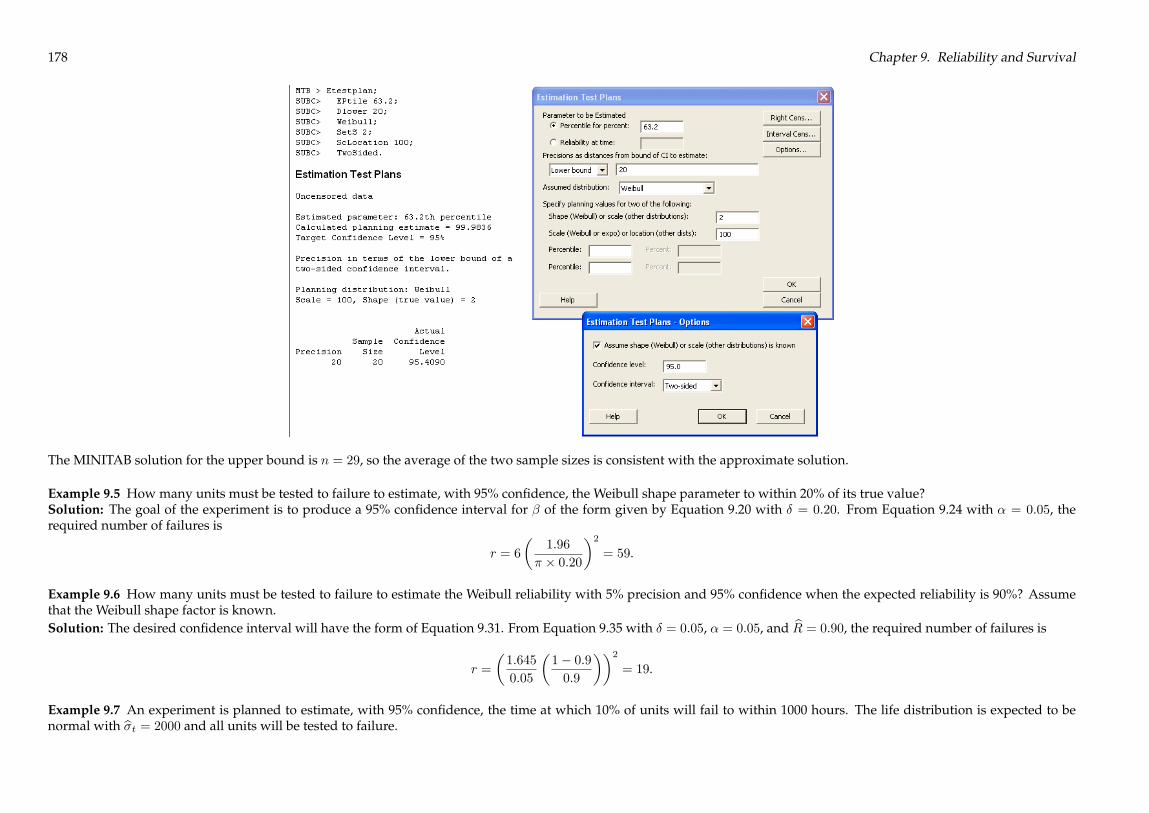
178 Chapter 9. Reliability and Survival
The MINITAB solution for the upper bound is n = 29, so the average of the two sample sizes is consistent with the approximate solution.
Example 9.5 How many units must be tested to failure to estimate, with 95% confidence, the Weibull shape parameter to within 20% of its true value?Solution: The goal of the experiment is to produce a 95% confidence interval for � of the form given by Equation 9.20 with � = 0:20. From Equation 9.24 with � = 0:05, therequired number of failures is
r = 6
�1:96
� � 0:20
�2= 59.
Example 9.6 How many units must be tested to failure to estimate the Weibull reliability with 5% precision and 95% confidence when the expected reliability is 90%? Assumethat the Weibull shape factor is known.Solution: The desired confidence interval will have the form of Equation 9.31. From Equation 9.35 with � = 0:05, � = 0:05, and bR = 0:90, the required number of failures is
r =
�1:645
0:05
�1� 0:90:9
��2= 19.
Example 9.7 An experiment is planned to estimate, with 95% confidence, the time at which 10% of units will fail to within 1000 hours. The life distribution is expected to benormal with b�t = 2000 and all units will be tested to failure.
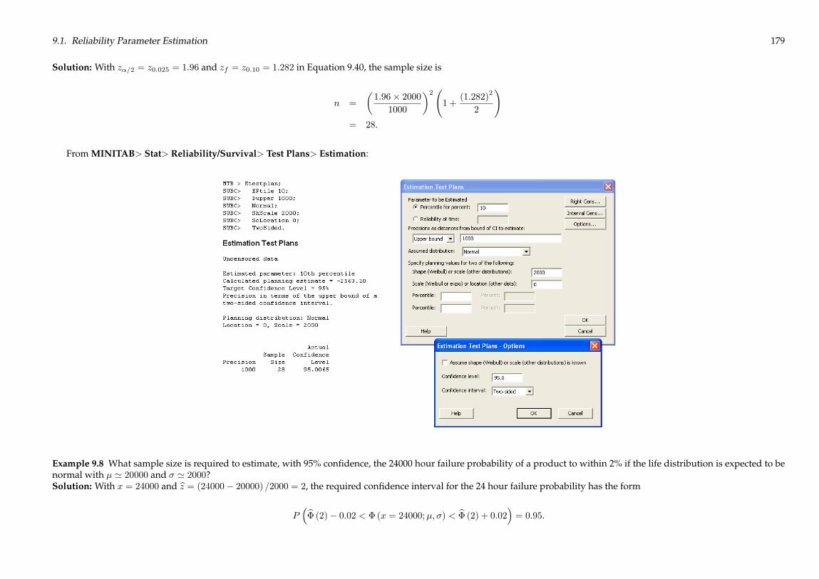
9.1. Reliability Parameter Estimation 179
Solution: With z�=2 = z0:025 = 1:96 and zf = z0:10 = 1:282 in Equation 9.40, the sample size is
n =
�1:96� 20001000
�2 1 +
(1:282)2
2
!= 28.
From MINITAB> Stat> Reliability/Survival> Test Plans> Estimation:
Example 9.8 What sample size is required to estimate, with 95% confidence, the 24000 hour failure probability of a product to within 2% if the life distribution is expected to benormal with � ' 20000 and � ' 2000?Solution: With x = 24000 and bz = (24000� 20000) =2000 = 2, the required confidence interval for the 24 hour failure probability has the form
P�b� (2)� 0:02 < � (x = 24000;�; �) < b� (2) + 0:02� = 0:95.
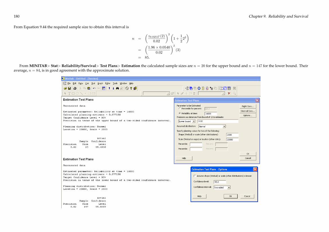
180 Chapter 9. Reliability and Survival
From Equation 9.44 the required sample size to obtain this interval is
n =
�z0:025' (2)
0:02
�2�1 +
1
222�
=
�1:96� 0:0540
0:02
�2(3)
= 85.
From MINITAB> Stat> Reliability/Survival> Test Plans> Estimation the calculated sample sizes are n = 20 for the upper bound and n = 147 for the lower bound. Theiraverage, n = 84, is in good agreement with the approximate solution.

9.2. Reliability Demonstration Tests 181
9.2 Reliability Demonstration Tests
Example 9.9 How many units must be tested for 200 hours without any failures to show, with 95% confidence, that theMTTF of a system exceeds 400 hours. The life distributionis exponential and the test is time terminated.Solution: We must determine the value of n with r = 0 failures in t0 = 200 hours of testing such that
P (400 < � <1) = 0:95.
From the f 0 equation for the exponential distribution from Table 9.1 with �0 = 400, the t0 = 200 hour failure probability is
f 0 = 1� e�t0=�0
= 1� e�200=400
= 0:3935.
With r = 0 and � = 0:05 the smallest value of n that satisfies Equation 9.46 is n = 6 because
(b (0; 6; 0:3935) = 0:04977) < (� = 0:05) .
From MINITAB> Stat> Reliability/Survival> Test Plans>Demonstration:
Example 9.10 Determine how long ten units must be life tested with no more than one failure during the test period to demonstrate, with 90% confidence, that the mean life isgreater than 1000 hours. Assume that the life distribution is exponential.Solution: The goal of the experiment is to demonstrate that
P (1000 < � <1) = 0:90.
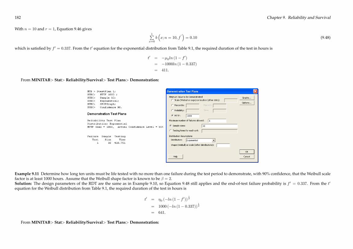
182 Chapter 9. Reliability and Survival
With n = 10 and r = 1, Equation 9.46 gives1P
x=0b�x;n = 10; f
0�= 0:10 (9.48)
which is satisfied by f 0 = 0:337. From the t0 equation for the exponential distribution from Table 9.1, the required duration of the test in hours is
t0 = ��0ln (1� f 0)= �1000ln (1� 0:337)= 411.
From MINITAB> Stat> Reliability/Survival> Test Plans>Demonstration:
Example 9.11 Determine how long ten units must be life tested with no more than one failure during the test period to demonstrate, with 90% confidence, that the Weibull scalefactor is at least 1000 hours. Assume that the Weibull shape factor is known to be � = 2:Solution: The design parameters of the RDT are the same as in Example 9.10, so Equation 9.48 still applies and the end-of-test failure probability is f 0 = 0:337. From the t0
equation for the Weibull distribution from Table 9.1, the required duration of the test in hours is
t0 = �0 (�ln (1� f 0))1�
= 1000 (�ln (1� 0:337))12
= 641.
From MINITAB> Stat> Reliability/Survival> Test Plans>Demonstration:
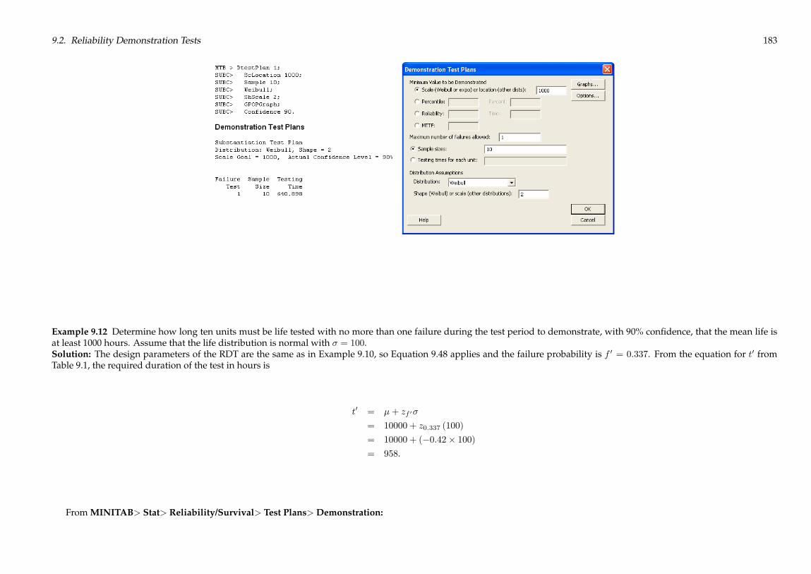
9.2. Reliability Demonstration Tests 183
Example 9.12 Determine how long ten units must be life tested with no more than one failure during the test period to demonstrate, with 90% confidence, that the mean life isat least 1000 hours. Assume that the life distribution is normal with � = 100.Solution: The design parameters of the RDT are the same as in Example 9.10, so Equation 9.48 applies and the failure probability is f 0 = 0:337. From the equation for t0 fromTable 9.1, the required duration of the test in hours is
t0 = �+ zf 0�
= 10000 + z0:337 (100)
= 10000 + (�0:42� 100)= 958.
From MINITAB> Stat> Reliability/Survival> Test Plans>Demonstration:

184 Chapter 9. Reliability and Survival
Example 9.13 How many units must be tested for 400 hours without any failures to demonstrate 90% reliability at 600 hours , with 95% confidence? Assume that the reliabilitydistribution is exponential.Solution: In terms of the 600 hour failure probability, the goal of the experiment is to demonstrate
P (0 < f (600) < 0:10) = 0:95
based on a sample of size n tested to t0 = 400 hours with r = 0 failures. From Table 9.2 the equation for f 0 for the exponential distribution gives
f 0 = 1� (1� f0)t0=t0
= 1� (1� 0:10)400=600
= 0:0678.
With r = 0, f 0 = 0:0678, and � = 0:05, Equation 9.46 gives
b (0;n; 0:0678) � 0:05,
which is satisfied by n = 43.
From MINITAB> Stat> Reliability/Survival> Test Plans>Demonstration:

9.2. Reliability Demonstration Tests 185
Example 9.14 How long must ten units be life tested with no more than one failure during the test period to demonstrate, with 80% confidence, that the 3000-hour reliability isat least 90%. Assume that the life distribution is Weibull with � = 1:8.Solution: The goal of the experiment is to demonstrate that
P (0:90 < R (3000) < 1) = 0:80
or in terms of the failure probabilityP (0 < f (3000) < 0:10) = 0:80.
With n = 10, r = 1, and � = 0:20, Equation 9.46 becomes1P
x=0b (x; 10; f 0) � 0:20,
which is satisfied by f 0 = 0:271. From the equation for t0 for the Weibull distribution from Table 9.2 with f0 = 0:10 and t0 = 3000, the test time is
t0 = t0
�ln (1� f 0)ln (1� f0)
�1=�= 3000
�ln (1� 0:271)ln (1� 0:10)
�1=1:8= 5523.
From MINITAB> Stat> Reliability/Survival> Test Plans>Demonstration:

186 Chapter 9. Reliability and Survival
Example 9.15 How many units must be tested for 140 hours with no more than one failure to demonstrate that the 100 hour reliability is at least 95% with 90% confidence?Assume that the reliability distribution is normal with � = 20.Solution: The goal of the experiment is to demonstrate
P (0 < f (100) < 0:05) = 0:90
based on a sample of size n tested to t0 = 140 hours with no more than r = 1 failures. From Table 9.2, the equation for zf 0 for the normal distribution gives
zf 0 = zf0 +
�t0 � t0�
�= z0:05 +
�140� 100
20
�= �1:645 + 2:0= 0:355,
which is satisfied by f 0 = �(�1 < z < 0:355) = 0:639. With r = 1, f 0 = 0:639, and � = 0:10, Equation 9.46 becomes
1Px=0
b (x;n; 0:639) � 0:10,
which is satisfied by n = 5.From MINITAB> Stat> Reliability/Survival> Test Plans>Demonstration:
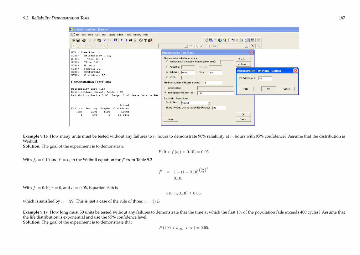
9.2. Reliability Demonstration Tests 187
Example 9.16 How many units must be tested without any failures to t0 hours to demonstrate 90% reliability at t0 hours with 95% confidence? Assume that the distribution isWeibull.Solution: The goal of the experiment is to demonstrate
P (0 < f (t0) < 0:10) = 0:95.
With f0 = 0:10 and t0 = t0 in the Weibull equation for f 0 from Table 9.2
f 0 = 1� (1� 0:10)�t0t0
��= 0:10.
With f 0 = 0:10, r = 0, and � = 0:05, Equation 9.46 isb (0;n; 0:10) � 0:05,
which is satisfied by n = 29. This is just a case of the rule of three: n = 3=f0.
Example 9.17 How long must 50 units be tested without any failures to demonstrate that the time at which the first 1% of the population fails exceeds 400 cycles? Assume thatthe life distribution is exponential and use the 95% confidence level.Solution: The goal of the experiment is to demonstrate that
P (400 < t0:01 <1) = 0:95.

188 Chapter 9. Reliability and Survival
From Equation 9.46 with r = 0, n = 50, and � = 0:05b (0; 50; f 0) � 0:05,
which is satisfied by f 0 = 0:058. From the exponential form of t0 from Table 9.2 with t0 = 400, the required duration of the test in cycles is
t0 = t0ln (1� f 0)ln (1� f0)
= 400ln (1� 0:058)ln (1� 0:01)
= 2380.
From MINITAB> Stat> Reliability/Survival> Test Plans>Demonstration:
Example 9.18 How many units must be tested to 30,000 cycles without any failures to demonstrate, with 95% confidence, that the 20,000 cycle reliability is at least 90%? The lifedistribution is known to be Weibull with � = 3:1.Solution: The goal of the experiment is to demonstrate that
P (20000 < t0:10 <1) = 0:95.
The equation for f 0 for the Weibull distribution from Table 9.2 with f0 = 0:10, t0 = 20000, t0 = 30000, and � = 3:1 gives
f 0 = 1� (1� f0)(t0=t0)
�
= 1� (1� 0:10)(30000=20000)3:1
= 0:3095.
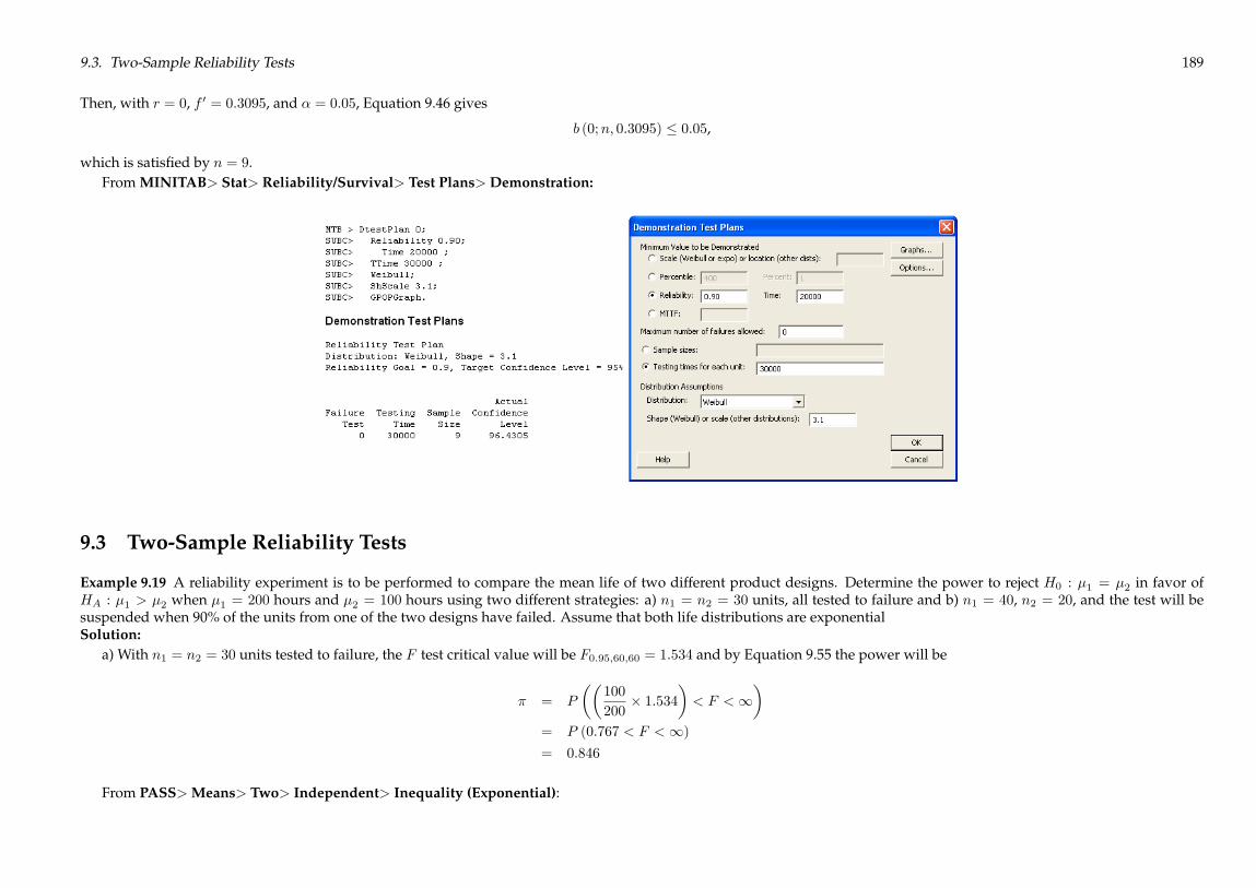
9.3. Two-Sample Reliability Tests 189
Then, with r = 0, f 0 = 0:3095, and � = 0:05, Equation 9.46 gives
b (0;n; 0:3095) � 0:05,
which is satisfied by n = 9.From MINITAB> Stat> Reliability/Survival> Test Plans>Demonstration:
9.3 Two-Sample Reliability Tests
Example 9.19 A reliability experiment is to be performed to compare the mean life of two different product designs. Determine the power to reject H0 : �1 = �2 in favor ofHA : �1 > �2 when �1 = 200 hours and �2 = 100 hours using two different strategies: a) n1 = n2 = 30 units, all tested to failure and b) n1 = 40, n2 = 20, and the test will besuspended when 90% of the units from one of the two designs have failed. Assume that both life distributions are exponentialSolution:
a) With n1 = n2 = 30 units tested to failure, the F test critical value will be F0:95;60;60 = 1:534 and by Equation 9.55 the power will be
� = P
��100
200� 1:534
�< F <1
�= P (0:767 < F <1)= 0:846
From PASS>Means> Two> Independent> Inequality (Exponential):
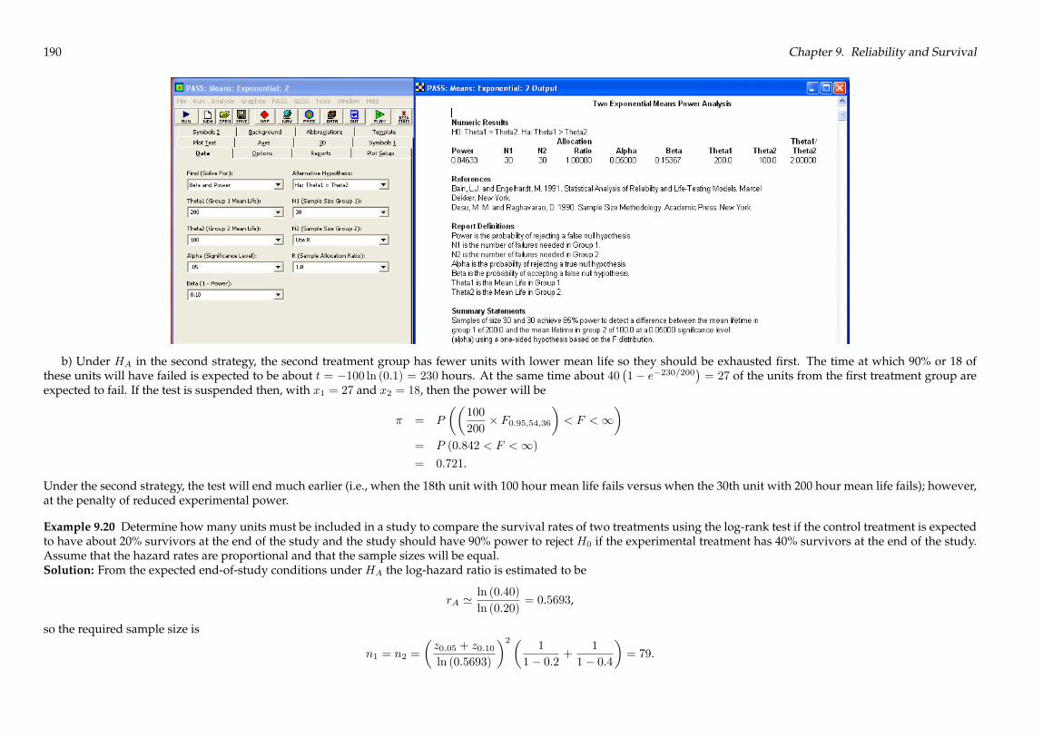
190 Chapter 9. Reliability and Survival
b) Under HA in the second strategy, the second treatment group has fewer units with lower mean life so they should be exhausted first. The time at which 90% or 18 ofthese units will have failed is expected to be about t = �100 ln (0:1) = 230 hours. At the same time about 40
�1� e�230=200
�= 27 of the units from the first treatment group are
expected to fail. If the test is suspended then, with x1 = 27 and x2 = 18, then the power will be
� = P
��100
200� F0:95;54;36
�< F <1
�= P (0:842 < F <1)= 0:721.
Under the second strategy, the test will end much earlier (i.e., when the 18th unit with 100 hour mean life fails versus when the 30th unit with 200 hour mean life fails); however,at the penalty of reduced experimental power.
Example 9.20 Determine how many units must be included in a study to compare the survival rates of two treatments using the log-rank test if the control treatment is expectedto have about 20% survivors at the end of the study and the study should have 90% power to reject H0 if the experimental treatment has 40% survivors at the end of the study.Assume that the hazard rates are proportional and that the sample sizes will be equal.Solution: From the expected end-of-study conditions under HA the log-hazard ratio is estimated to be
rA 'ln (0:40)
ln (0:20)= 0:5693,
so the required sample size is
n1 = n2 =
�z0:05 + z0:10ln (0:5693)
�2�1
1� 0:2 +1
1� 0:4
�= 79.

9.3. Two-Sample Reliability Tests 191
From PASS> Survival and Reliability> Log-Rank Survival (Simple):
Example 9.21 Compare the power of the log-rank test to the power of the two-sample test for exponential mean life for Example 9.19b.Solution: Because the hazard rate of an exponential distribution is constant, the proportional hazards assumption is satisfied. At 230 hours with s1 (t0) = 2=20 = 0:10 ands2 (t
0) = 13=40 = 0:325 the hazard ratio under HA will be
rA =ln (0:325)
ln (0:10)= 0:488.
With n2=n1 = 2, d1 (t0) = 18, and d2 (t0) = 27, the z� value from Equation 9.64 is
z� =1� 0:4881 + 2 (0:488)
p2 (18 + 27)� 1:96 = 0:50.
Then the power for the log-rank test is � = �(�1 < z < 0:50) ' 0:69, which is slightly less than the power for the two-sample exponential test for mean life, which was � = 0:72.The two-tailed test was used here to match the power obtained in Example 9.19.
From PASS> Survival and Reliability> Log-Rank Survival (Simple):

192 Chapter 9. Reliability and Survival
Example 9.22 Compare the sample size calculated by Lachin’s method to that of Schoenfeld’s method in Example 9.20.Solution: From the information given in the problem statement and Equation 9.66 the sample size by Lachin’s method must be
n1 = n2 =(1:645 + 1:282)
2
2� 0:2� 0:4
�1 + 0:5693
1� 0:5693
�2= 82,
which is in good agreement with Schoenfeld’s method, n = 79.See the NCSS/PASS solution shown in Example 9.20. The manual calculation by Schoenfeld’s method is in excellent agreement with PASS which uses the same method.
9.4 Interference
Example 9.23 A random sample of component strengths gave nS = 100, b�S = 600, and b�S = 60 and a random sample of loads gave nL = 36, b�L = 450, and b�L = 40. Bothdistributions are known to be normal. Determine the 90% upper confidence limit for the interference failure rate.Solution: The point estimate for bzf is given by Equation 9.73: bzf = 450� 600p
402 + 602= �2:08
and the corresponding point estimate for the interference failure rate is
bf = �(�1 < z < �2:08) = 0:0188.
The approximate standard deviation of the bzf distribution is given by Equation 9.74:
b�bzf =vuut 1
402 + 602
402
36+602
100+1
2
�450� 600402 + 602
�2�404
36+604
100
�!= 0:178.

9.4. Interference 193
Then, from Equation 9.76 with z0:10 = 1:282 bzfU = �2:08 + 1:282� 0:178= �1:85,
so from Equation 9.75 the 90% upper confidence limit for the interference failure probability is
bfU = �(�1 < z < �1:85)= 0:032.
That is, on the basis of the sample data, we can claim that the one-sided upper 90% confidence interval for the interference failure rate is
P (0 < f < 0:032) = 0:90.
Example 9.24 What sample size is required to demonstrate that the interference failure probability is less than 0.1% with 90% confidence if the strength distribution is known tobe normal with �S = 20 and �S = 2 and the load distribution is expected to be normal with b�L = 13 and b�L = 1?Solution: The point estimate for the interference failure probability determined from the S parameters and the L parameter estimates is
bf = �(�1 < z < bzf )= �
��1 < z <
13� 20p12 + 22
�= �(�1 < z < �3:13)= 0:000874.
The sample size required to study the load distribution is given by swapping the relevant S and L subscripts in Equation 9.78:
nL =
�z�bzfU � bzf
�2 b�2Lb�2L + �2S!0@1 + b�2L
2
b�L � �Sb�2L + �2S!21A (9.1)
=
�z0:10
z0:001 � z0:000874
�2�12
12 + 22
� 1 +
12
2
�13� 2012 + 22
�2!
=
�1:282
�3:09� (�3:13)
�2�12
12 + 22
� 1 +
12
2
�13� 2012 + 22
�2!= 407.
Example 9.25 What sample size is required to determine the 95% two-sided confidence interval for the exponential-exponential interference failure rate if the confidence limitsmust be within 50% of the predicted mean failure rate?Solution: The goal of the experiment is to obtain a confidence interval for the exponential-exponential interference failure rate f of the form
��0:50 bf < f < 1:50 bf� = 0:95.

194 Chapter 9. Reliability and Survival
With z0:025 = 1:96 and � = 0:50 in Equation 9.90, the required equal sample sizes are
nL = nS = 2
�1:96
0:50
�2= 31.
Example 9.26 How many measurements of mating components in a device must be taken to demonstrate, with 95% confidence, that their true interference failure rate does notexceed the observed failure rate by 20% if the two distributions are known to be Weibull with �S = 2:5 and �L = 1:5, respectively?Solution: The goal of the experiment is to acquire sufficient information to demonstrate the following one-sided upper confidence interval for the interference failure rate f :
P�0 < f < bf (1 + 0:2)� = 0:95.
With � = 0:2 and � = 0:05 in Equation 9.100, we obtain the sample size
n =
1:645
0:2� ��1 + 2:5
1:5
�!2�1 + 2:521:52
�= 113.

Chapter 10
Statistical Quality Control
10.1 Statistical Process Control
Example 10.1 Evaluate the following control chart run rule: A process is judged to be out of control if at least two of three consecutive observations falls beyond the same 2�limit on the chart.Solution: The rule is easy to identify on the chart, so it satisfies the first condition for a valid run rule. If the process is in control and the distribution of the statistic (call it w) isapproximately normal, then the probability that any point on the chart falls above �w+2�w is p = �(2 < z <1) = 0:023. The probability that at least x = 2 of n = 3 consecutivepoints fall above that limit is given by the binomial probability
3Px=2
b (x;n = 3; p = 0:023) = 0:0016.
Because this pattern could also appear on the bottom half of the chart, the type I error rate for this rule is � = 2 (0:0016) = 0:0032, which is acceptably low, so the rule meets thesecond requirement for a valid control chart rule. If the process mean shifted to �w +2�w, then the probability that an observation would fall beyond �w +2�w is p = 0:5 and thecorresponding power of the rule is
� =3P
x=2b (x;n = 3; p = 0:5) = 0:5.
This meets the third requirement of a valid control chart rule. Because all three conditions are satisfied, that is: 1) the rule is easy to recognize, 2) it has a low type I error rate,and 3) it has good power to detect shifts in the process, then it is a valid control chart run rule.
Example 10.2 One of the weaknesses of defects charts when the sampling unit is small is that it is not possible to declare a process to be out of control on the lower side of thechart with a single observation. Evaluate the following special run rule for defects charts: If a defects chart’s sampling unit size is sufficient to deliver � � 3, then the process isout of control if two consecutive sampling units have 0 defects.Solution: The chart obviously meets the first and third conditions for valid control chart run rules, but it is not clear if the second condition (low type I error rate) is satisfied.If the mean defect rate is � = 3, then the probability of a sampling unit having 0 defects when the process is in control (H0 : � = 3) is Poisson (x = 0;� = 3) = 0:05, a rathercommon occurrence. Under the same conditions, the probability of observing two consecutive zeros is b (x = 2;n = 2; p = 0:05) = 0:0025, but this is just the type I error rate forthe rule. Because � = 0:0025 is acceptably low, the rule meets all three conditions for a valid control chart run rule.
195
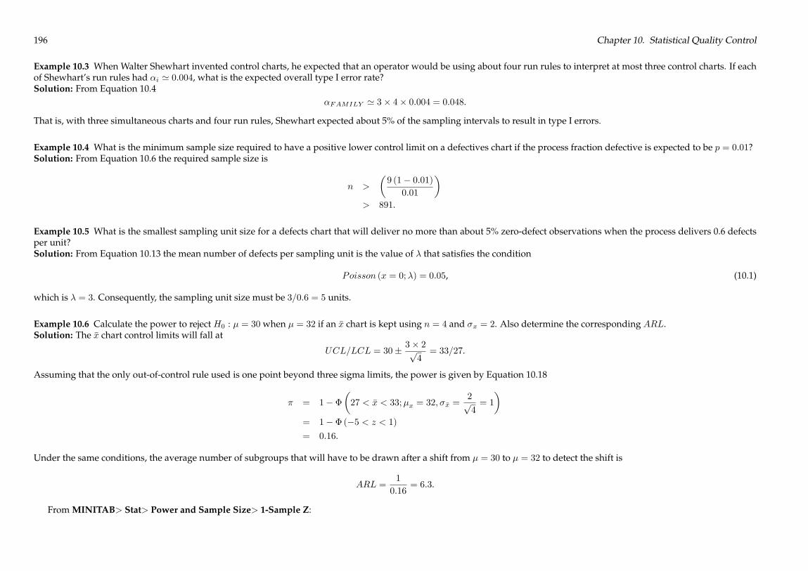
196 Chapter 10. Statistical Quality Control
Example 10.3 When Walter Shewhart invented control charts, he expected that an operator would be using about four run rules to interpret at most three control charts. If eachof Shewhart’s run rules had �i ' 0:004, what is the expected overall type I error rate?Solution: From Equation 10.4
�FAMILY ' 3� 4� 0:004 = 0:048.
That is, with three simultaneous charts and four run rules, Shewhart expected about 5% of the sampling intervals to result in type I errors.
Example 10.4 What is the minimum sample size required to have a positive lower control limit on a defectives chart if the process fraction defective is expected to be p = 0:01?Solution: From Equation 10.6 the required sample size is
n >
�9 (1� 0:01)
0:01
�> 891.
Example 10.5 What is the smallest sampling unit size for a defects chart that will deliver no more than about 5% zero-defect observations when the process delivers 0.6 defectsper unit?Solution: From Equation 10.13 the mean number of defects per sampling unit is the value of � that satisfies the condition
Poisson (x = 0;�) = 0:05, (10.1)
which is � = 3. Consequently, the sampling unit size must be 3=0:6 = 5 units.
Example 10.6 Calculate the power to reject H0 : � = 30 when � = 32 if an �x chart is kept using n = 4 and �x = 2. Also determine the corresponding ARL.Solution: The �x chart control limits will fall at
UCL=LCL = 30� 3� 2p4= 33=27.
Assuming that the only out-of-control rule used is one point beyond three sigma limits, the power is given by Equation 10.18
� = 1� ��27 < �x < 33;�x = 32; ��x =
2p4= 1
�= 1� � (�5 < z < 1)= 0:16.
Under the same conditions, the average number of subgroups that will have to be drawn after a shift from � = 30 to � = 32 to detect the shift is
ARL =1
0:16= 6:3.
From MINITAB> Stat> Power and Sample Size> 1-Sample Z:

10.2. Process Capability 197
10.2 Process Capability
Example 10.7 What sample size is required to determine cp to within 10% of its true value with 90% confidence?Solution: With � = 0:10 and � = 0:10 in Equation 10.26 the required sample size is
n =1
2
�1:645
0:10
�2= 136.
The cp value is inversely proportional to the standard deviation, so a standard deviation calculator can be used to determine the sample size required for a confidence intervalfor cp. From PASS> Variance> Variance: 1 Group:

198 Chapter 10. Statistical Quality Control
Example 10.8 What sample size is required to estimate cpk to within 5% of its true value with 90% confidence if cpk = 1:0 is expected?Solution: From Equation 10.30 with � = 0:05 and � = 0:05 the required sample size is
n '�1:645
0:05
�2 1
9 (1:0)2 +
1
2
!= 662.
Example 10.9 What sample size is required to estimate cpk to within 5% of its true value with 90% confidence if cpk is expected to be very large?Solution: From Equation 10.31 with � = 0:05 and � = 0:05 the required sample size is
n ' 1
2
�1:645
0:05
�2= 541.
Example 10.10 Determine the sample size required to reject H0 : cp = 1:33 in favor of HA : cp > 1:33with 90% power when cp = 1:5.Solution: With (cp)0 = 1:33, (cp)1 = 1:5, � = 0:05, and � = 0:10 in Equation 10.33, the required sample size is
n ' 1
2
1:645 + 1:282
ln�1:51:33
� !2= 297.
The hypothesis test for cp can be performed using a sample size calculator for the standard deviation. By setting the standard deviations to the reciprocals of cp in PASS>Variance> Variance: 1 Group:
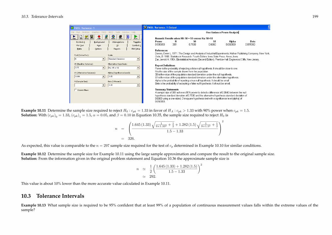
10.3. Tolerance Intervals 199
Example 10.11 Determine the sample size required to reject H0 : cpk = 1:33 in favor of HA : cpk > 1:33with 90% power when cpk = 1:5.Solution: With (cpk)0 = 1:33, (cpk)1 = 1:5, � = 0:05, and � = 0:10 in Equation 10.35, the sample size required to reject H0 is
n =
0@1:645 (1:33)q
19�1:332 +
12 + 1:282 (1:5)
q1
9�1:52 +12
1:5� 1:33
1A2
= 326.
As expected, this value is comparable to the n = 297 sample size required for the test of cp determined in Example 10.10 for similar conditions.
Example 10.12 Determine the sample size for Example 10.11 using the large sample approximation and compare the result to the original sample size.Solution: From the information given in the original problem statement and Equation 10.36 the approximate sample size is
n ' 1
2
�1:645 (1:33) + 1:282 (1:5)
1:5� 1:33
�2' 292.
This value is about 10% lower than the more accurate value calculated in Example 10.11.
10.3 Tolerance Intervals
Example 10.13 What sample size is required to be 95% confident that at least 99% of a population of continuous measurement values falls within the extreme values of thesample?

200 Chapter 10. Statistical Quality Control
Solution: With � = 0:05 and pU = 0:01 the required sample size is approximately
n '�20:95;42� 0:01
' 475.
Further iterations indicate that the smallest value of n for which � � 0:05 is n = 473, which leads to the following nonparametric tolerance interval for x:
P (0:99 < P (xmin � x � xmax) < 1) = 0:9502.
Example 10.14 What sample size n is required to be 95% confident that at least 99% of a population of continuous measurement values falls below the maximum value of thesample?Solution: With � = 0:05 and pU = 0:01 the required sample size is
n '�20:95;22� 0:01
' 300.
Example 10.15 Determine the sample size required to obtain a 95% confidence two-sided 99% coverage normal distribution tolerance interval with tolerance limits UTL=LTL =�x� 3:5s.Solution: The desired tolerance interval has the form
P (0:99 � � (�x� 3:5s � x � �x+ 3:5s) � 1) = 0:95.
From Appendix E.7, as sample of size n = 25 gives k2 = 3:46. A spreadsheet (not shown) was set up to calculate k2 as a function of n using Equation 10.47 with p = 0:01 and� = 0:05. The spreadsheet indicated that the sample size n = 24 delivers k2 = 3:485 and that n = 23 delivers k2 = 3:514, so n = 24 should be used to be conservative. Theseapproximate k2 values differ from the exact values given in Appendix E.7 in the thousandths place.
Example 10.16 Determine the sample size required to obtain a 95% confidence 99% coverage normal distribution tolerance interval with one-sided upper tolerance limit UTL =�x+ 3s.Solution: The required interval has the form
P (0:99 < � (�1 < x � UTL) < 1) = 0:95 (10.2)
where UTL = �x+ k1swith k1 = 3. From Table E.7 of Appendix E with � = 0:05 and Y = 0:99, the required sample size is n = 35.
10.4 Acceptance Sampling
Example 10.17 Design the single sampling plan for attributes that will accept 95% of lots when the process fraction defective is 1% and accept only 10% of lots when the processfraction defective is 5%.Solution: From the problem statement, the lots are coming from a continuous process, so the sampling plan will be Type B with points on the OC curve at (AQL; 1� �) =

10.4. Acceptance Sampling 201
(0:01; 0:95) and (RQL; �) = (0:05; 0:10). From Table 10.1 with RQL=AQL = 0:05=0:01 = 5:0, the acceptance number must be c = 3. Then, from the RQL condition, the requiredsample size is approximately
n '�20:90;82 (0:05)
' 13:36
2� 0:05' 134.
The exact sampling plan that meets the specifications in the problem statement is n = 132 and c = 3.From MINITAB> Stat>Quality Tools> Acceptance Sampling by Attributes:
Example 10.18 Find the c = 0 plans that meet a) the AQL requirement and b) the RQL requirement from Example 10.17. Plot the three OC curves on the same graph.Solution:
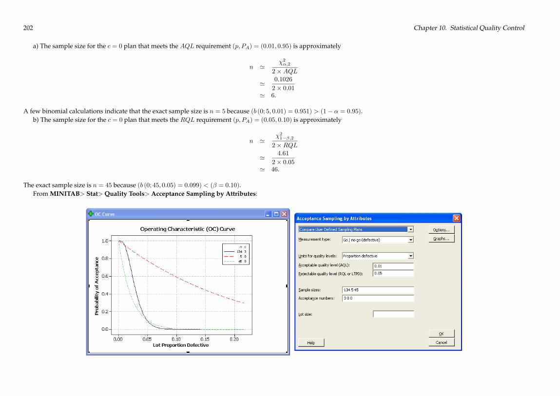
202 Chapter 10. Statistical Quality Control
a) The sample size for the c = 0 plan that meets the AQL requirement (p; PA) = (0:01; 0:95) is approximately
n '�2�;2
2�AQL
' 0:1026
2� 0:01' 6.
A few binomial calculations indicate that the exact sample size is n = 5 because (b (0; 5; 0:01) = 0:951) > (1� � = 0:95).b) The sample size for the c = 0 plan that meets the RQL requirement (p; PA) = (0:05; 0:10) is approximately
n '�21��;22�RQL
' 4:61
2� 0:05' 46.
The exact sample size is n = 45 because (b (0; 45; 0:05) = 0:099) < (� = 0:10).From MINITAB> Stat>Quality Tools> Acceptance Sampling by Attributes:

10.4. Acceptance Sampling 203
Example 10.19 Determine the sampling plan for lots of size N = 50 that will accept 95% of the lots with D � 1 defectives and reject 90% of the lots with D � 5 defectives.Solution: The sampling plan must meet the simultaneous conditions given by Equation 10.57 with D1 = 1 and � � 0:05:
cPx=0
h (x;D1 = 1; N = 50; n) � 0:95 (10.3)
and Equation 10.58 with D2 = 5 and � � 0:10:
cPx=0
h (x;D2 = 5; N = 50; n) < 0:10. (10.4)
The acceptance number c is not specified, so different values of cmust be considered. The approximate sample size for the c = 0 sampling plan to meet the condition in Equation10.63 is given by Equation 10.61:
n ' 50�1� 0:101=5
�= 19;
however, the condition in Equation 10.62 is not satisfied because
(h (x = 0;D1 = 1; N = 50; n = 19) = 0:525) � 0:95.
Iterations with a hypergeometric calculator show that with c = 1 Equation 10.63 is satisfied when n = 29 because
�1P
x=0h (x;D1 = 5; N = 50; n = 28) = 0:109
�� 0:10�
1Px=0
h (x;D1 = 5; N = 50; n = 29) = 0:092
�� 0:10
and Equation 10.62 is satisfied because �1P
x=0h (x;D1 = 1; N = 50; n = 29) = 1
�� 0:95.
The sampling plan that meets the requirements is n = 29with c = 1.
From MINITAB> Stat>Quality Tools> Acceptance Sampling by Attributes:

204 Chapter 10. Statistical Quality Control
Example 10.20 A 100% inspection process for large lots is to be replaced with a c = 0 sampling plan. What fraction of each lot must be inspected if lots that contain five or moredefectives must be rejected 90% of the time?Solution: From Equation 10.61 with D = 5 and PA = 0:10, the fraction of each lot that must be inspected is
n
N' 1� 0:101=5
' 0:37.
Example 10.21 The calculated sample size in Example 4.2 was quite large compared to the lot size, which violates the small-sample approximation assumption. Repeat thatexample using the small-lot-size method.Solution: The solution in the example indicated that 30% of the lot needed to be inspected. From Equation 10.61, which takes the relatively large sample size into account, thefraction of the lot that has to be inspected is more accurately
n
N' 1� 0:051=10
' 0:259.
10.4. Acceptance Sampling 205
Example 10.22 Create the OC curves for normal, tightened, and reduced inspection under ANSI/ASQ Z1.4 using general inspection level II, single sampling, N = 1000, andAQL = 1%.Solution: The sampling plans determined for code letter J from the standard were normal (n = 200; c = 5), tightened (n = 200; c = 3), and reduced (n = 80; c = 2). The operatingcharacteristic curves were calculated using Equation 10.54 and are shown in Figure 10.6. For reference, the figure also shows the OC curve for the sampling plan determined forthe same conditions using the Squeglia zero acceptance number sampling standard, which is often used instead of ANSI/ASQ Z1.4.
Example 10.23 Determine the optimal rectifying inspection sampling plan for LTPD = 0:04 with � = 0:10 when the lot size is N = 2500 and the historical process fractiondefective is p = 0:01.Solution: A spreadsheet was used to solve Equations 10.66 and 10.67 as a function of acceptance number c as shown in Table 10.2. For the specified conditions, the samplingplan that minimizes ATI when p = 0:01 is n = 232 with c = 5. By comparison, the Dodge-Romig LTPD tables indicate a sampling plan with n = 230 and c = 5, which is inexcellent agreement with the calculated plan.
From MINITAB> Stat>Quality Tools> Acceptance Sampling by Attributes:

206 Chapter 10. Statistical Quality Control
Example 10.24 Find the rectifying inspection plan with LTPD = 0:04 and � = 0:1 for a lot size of N = 50.Solution: For the given conditions, the spreadsheet method gives n = 58, which exceeds the lot size. From Equation 10.70 the sample size required for the c = 0 plan is
n ' 50�1� 0:1 1
50�0:04
�' 35.
By comparison, the corresponding Dodge-Romig plan calls for n = 34 and is independent of the historical fraction defective.From MINITAB> Stat>Quality Tools> Acceptance Sampling by Attributes:

10.4. Acceptance Sampling 207
Example 10.25 What sample size is required for a c = 1 rectifying inspection single-sampling plan to obtain 1% AOQL if the lot size is N = 300? For what value of incomingfraction defective will AOQ be a maximum?Solution: From Equation 10.76 with A1 = 0:839 the required sample size is
n =1
0:010:839 +
1300
= 66.
AOQwill be at its maximum value, AOQL, when the incoming fraction defective is
pc =�212n=
3:24
2� 66 = 0:0245.
Example 10.26 Determine the sampling plan that minimizes the ATI for lots of size N = 1000with AOQL = 0:02 when the historical defective rate is p = 0:01.Solution: A spreadsheet was used to solve for n and ATI as a function of c using Equations 10.76 and 10.67. The results from the spreadsheet, shown in Table 10.4, indicate thatthe sampling plan that minimizes ATI is given by n = 65 and c = 2. By comparison, this is exactly the same plan indicated in the Dodge-Romig tables for these conditions.
208 Chapter 10. Statistical Quality Control
Example 10.27 Find the single sampling plan for variables that will accept 95% of the lots with 1% defectives and reject 90% of the lots with 4% defectives when � = 30 and thespecification is one-sided with USL = 700.Solution: The two specified points on the OC curve are (p0; 1� �) = (0:01; 0:95) and (p1; �) = (0:04; 0:10). From Equation 10.79 the required sample size is
n =
�z0:05 + z0:10z0:01 � z0:04
�2=
�1:645 + 1:282
2:33� 1:75
�2= 26.
The critical value of �xA=R is
�xA=R = �0 + z���x
= (USL� zp0�x) + z��xpn
= (700� 2:33� 30) + 1:645 30p26
= 640.
From MINITAB> Stat>Quality Tools> Acceptance Sampling by Variables> Create/Compare:
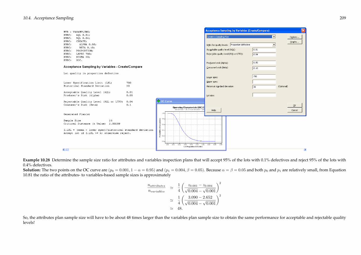
10.4. Acceptance Sampling 209
Example 10.28 Determine the sample size ratio for attributes and variables inspection plans that will accept 95% of the lots with 0.1% defectives and reject 95% of the lots with0.4% defectives.Solution: The two points on the OC curve are (p0 = 0:001; 1� � = 0:95) and (p1 = 0:004; � = 0:05). Because � = � = 0:05 and both p0 and p1 are relatively small, from Equation10.81 the ratio of the attributes- to variables-based sample sizes is approximately
nattributesnvariables
' 1
4
�z0:001 � z0:004p0:004�
p0:001
�2' 1
4
�3:090� 2:652p0:004�
p0:001
�2' 48.
So, the attributes plan sample size will have to be about 48 times larger than the variables plan sample size to obtain the same performance for acceptable and rejectable qualitylevels!

210 Chapter 10. Statistical Quality Control
Example 10.29 Find the single sampling plan for variables that will accept 95% of the lots with 1% defectives and reject 90% of the lots with 4% defectives. The specification isone-sided and � is unknown.Solution: The two specified points on the OC curve are (p0; 1� �) = (0:01; 0:95) and (p1; �) = (0:04; 0:10). From Equation 10.86, the condition that determines the sample size is
t0:95;n�1;�z0:01pn = t0:10;n�1;�z0:04pn ,
which is satisfied by n = 78 becauset0:95;77;�20:58 = t0:10;77;�15:46 = �17:75.
The accept/reject value of k for the test is
k =17:75p78
= 2:01.
From MINITAB> Stat>Quality Tools> Acceptance Sampling by Variables> Create/Compare:
Example 10.30 Plot the OC curves for the normal, tightened, and reduced sampling plans under ANSI/ASQ Z1.9 using a one-sided specification with Form 1, code letter F, andAQL = 1%.
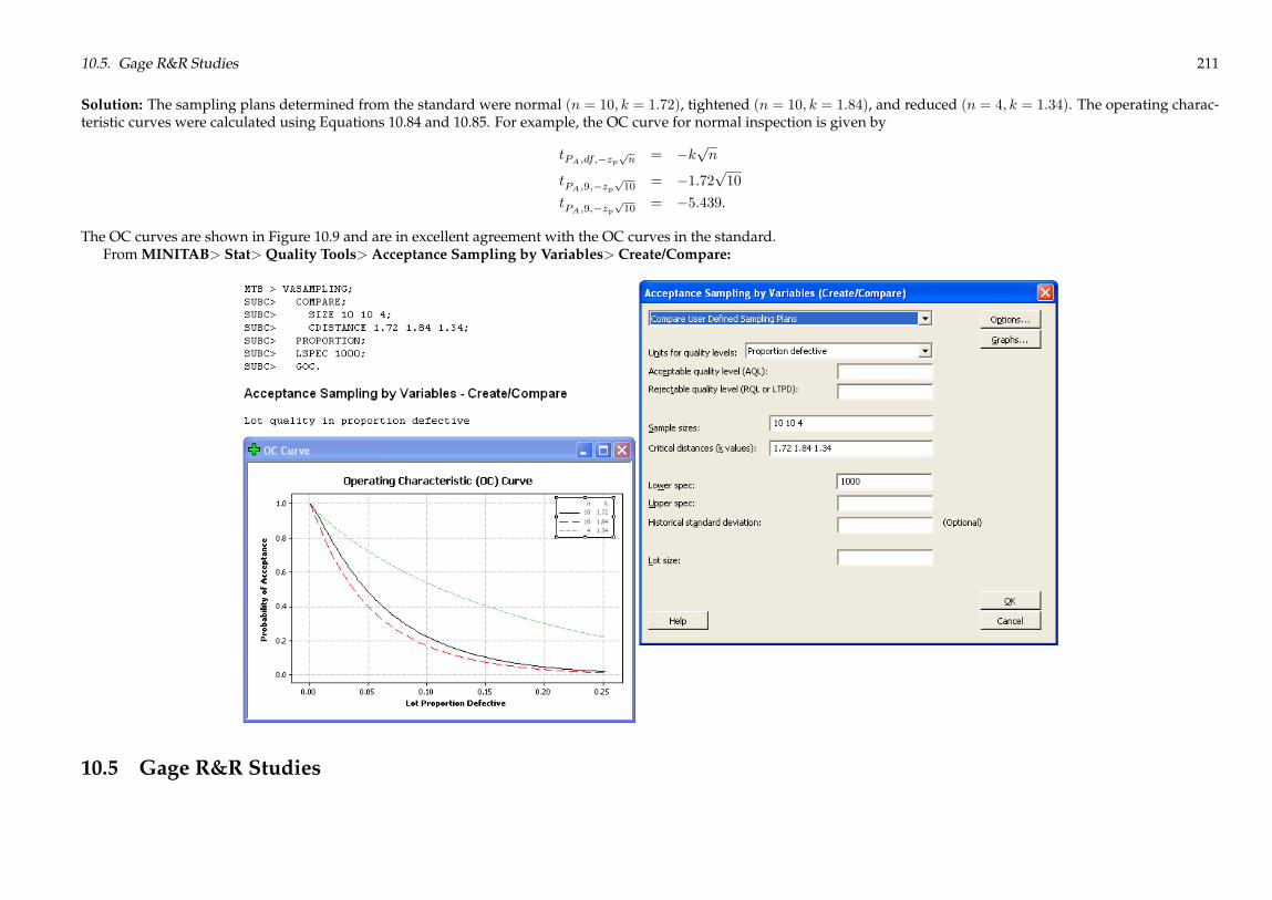
10.5. Gage R&R Studies 211
Solution: The sampling plans determined from the standard were normal (n = 10; k = 1:72), tightened (n = 10; k = 1:84), and reduced (n = 4; k = 1:34). The operating charac-teristic curves were calculated using Equations 10.84 and 10.85. For example, the OC curve for normal inspection is given by
tPA;df;�zppn = �k
pn
tPA;9;�zpp10 = �1:72
p10
tPA;9;�zpp10 = �5:439.
The OC curves are shown in Figure 10.9 and are in excellent agreement with the OC curves in the standard.From MINITAB> Stat>Quality Tools> Acceptance Sampling by Variables> Create/Compare:
10.5 Gage R&R Studies

212 Chapter 10. Statistical Quality Control
Chapter 11
Resampling Methods
11.1 Software Requirements
11.2 Monte Carlo
Example 11.1 How many samples should be drawn from a Poisson population to estimate the mean with 20% precision and 95% confidence? The mean is expected to be � = 5.Solution: The sample size must be sufficient to deliver the following confidence interval for �:
P�0:8b� < � < 1:2b�� = 0:95
P (4 < � < 6) = 0:95
where b� = x=n and x is the number of counts observed in n sampling units. A MINITAB macro was used to draw 10000 random samples, all of size n, from a Poisson distributionwith � = 5, and calculate b� for each sample. The 2:5th and 97:5th b� percentiles were used to estimate the 95% confidence limits. Figure 11.1 shows the Monte Carlo confidencelimits as a function of sample size. The sample size that delivers the desired confidence interval width is n = 19, which is in good agreement with the sample size given byEquation 5.11:
n =1
�
�z�=2�
�2=
1
5
�1:96
0:2
�2= 20.
Example 11.2 Use the Monte Carlo method to confirm the answer to Example 9.25, that samples of size n = 31 are required to estimate, with 95% confidence, the exponential–exponential interference failure rate to within �50%.Solution: A MINITAB macro was written that draws random samples of size n = 31 for exponential load and strength distributions, where the load distribution has mean �L,
213

214 Chapter 11. Resampling Methods
where �L comes from a uniform distribution with 1 � �L � 10, and the strength distribution has mean �S = k�L, where k comes from a uniform distribution with 3 � k � 10.The macro loops 1000 times, collecting the ratio of the empirical interference failure rate bf to the known failure rate f from each pass. Figure 11.2 shows the histogram of bf=f .About 97% of the observed bf values fall within �50% of their known f values, which is consistent with the intended 95% confidence level.
Example 11.3 An experiment is proposed to study the defective rate (p) of a process using a sample of size n = 300 units. The process is considered to be acceptable whenp � 0:01, but p � 0:03 is unacceptable. Determine the acceptance number and power for the sampling plan.Solution: The hypotheses to be tested areH0 : p � 0:01 versusHA : p > 0:01. The decision to rejectH0 or not is based on the observed number of defectives x in a sample of sizen = 300. The critical value of x that distinguishes the accept and reject regions should be chosen such that � � 0:05 for p = 0:01. To determine this critical value, MINITAB wasused to select 10000 random samples from a binomial population with n = 300 and p = 0:01. The frequencies and cumulative percentages by x are shown in the H0 columns ofTable 11.1. From the CumPct column, the critical value of x must be set to xA=R = 6:5 to provide good protection against type I errors (� = 1� 0:9692 = 0:0308). The frequencystatistics under HA in the Figure were created by selecting 10000 random samples from a binomial population with n = 300 and p = 0:03. From the CumPct column, the type IIerror probability relative to xA=R = 6:5 is � = 0:206, so the power to reject H0 when p = 0:03 is � = 1 � � = 0:794. This is in excellent agreement with the power calculated forthe one-sample proportion test (see Section 4.1.2), which is � = 0:797.
Example 11.4 Tukey’s quick test is a nonparametric two-sample test for location that is easy to perform using dotplots. The samples must be comparable in size and they mustbe slipped, that is, one sample must have the largest observation and the other sample must have the smallest observation. The test statistic, T , is the number of slipped ornonoverlapping points. The Tukey test rejects H0 : �1 = �2 when T � 7. For example, in Figure 11.3 T = 7 + 10 = 17, so there is sufficient evidence to reject H0.
Use the Monte Carlo method to determine the power of Tukey’s quick test as a function of effect size and sample size assuming that the two populations are normal andhomoscedastic.Solution: A MINITAB macro was written to draw 1000 random samples of equal sample size from two independent homoscedastic normal populations and count the numberof times thatH0 was rejected by the Tukey quick test. Figure 11.4 shows that the power of the test is low for all sample sizes until the difference between the means is greater than1.5 to 2.5 standard deviations. When the sample size is n � 20, Tukey’s quick test has power � � 0:90 for differences between the means of 1.5 standard deviations or greater.
11.3 Bootstrap
Example 11.5 The following yield strength values (in thousands of psi) for a material were obtained in a pilot study: {56, 23, 25, 68, 35, 31, 13, 15, 48, 37, 57, 69, 50, 76, 50, 19, 88,33, 10, 21}. What sample size is required to estimate, with 95% confidence, the mean yield strength to within �5000 psi?Solution: The bootstrap percentile confidence interval width was studied as a function of sample size using 1000 resamples for sample sizes from n = 30 to 100. Figure 11.5shows the confidence interval width, given by
2� = b��0:975 � b��0:025,
versus sample size. The sample size required to obtain the desired precision of the estimate is n = 75.
Example 11.6 The following data were obtained from a pilot study: {56, 48, 44, 62, 50, 47, 49, 57, 48, 55, 96, 47, 46, 47, 49, 72, 46, 61}. Determine the sample size required to obtain90% power to reject H0 : � = 50when � = 52. The population is not normal, so assume that the experimental data will be analyzed using the bootstrap method.
Solution: If the population distribution is normal, the one-sample Student’s t test would be an appropriate method of analysis. Because the normality assumption is not satisfied,the preferred method of analysis using the bootstrap method uses the analogous bootstrap-t distribution given by
t� =�x� � �0s�=pn
(11.4)

11.3. Bootstrap 215
where �x� and s� are the mean and standard deviation of bootstrap samples. Figure 11.6 shows the bootstrap distributions of t� with samples of size n = 18 under H0 : � = 50and HA : � = 56, where the sample data were shifted to the appropriate population means before bootstrapping using transformations of the form
x0i = xi � �x+ �.
From the bootstrap-t distribution under H0, the acceptance interval for H0 is �4:29 � t� � 1:62. The acceptance interval is skewed because the original sample is skewed. Fromthe bootstrap distribution under HA, the power is � = 0:802, which does not meet the 90% power requirement.
Figure 11.7 shows the bootstrap-t test power versus sample size for samples from size n = 16 to 30. (Figure 11.6 was constructed from 1000 bootstrap samples. Each point inFigure 11.7 was constructed from 10000 bootstrap samples to reduce the noise in the power versus sample size plot.) The sample size required to obtain 90% power to reject H0when � = 56 is n = 23.