Salt Solubility Products of Diprenorphine Hydrochloride ... · Salt Solubility Products of...

doi: 10.5599/admet.1.4.24 48

ADMET & DMPK 1(4) (2013) 48-62; doi: 10.5599/admet.1.4.24

Open Access : ISSN : 1848-7718

http://www.pub.iapchem.org/ojs/index.php/admet/index

Original scientific paper

Salt Solubility Products of Diprenorphine Hydrochloride,

Codeine and Lidocaine Hydrochlorides and Phosphates – Novel

Method of Data Analysis Not Dependent on Explicit Solubility

Equations

Gergely Völgyi1, Attila Marosi

1, Krisztina Takács-Novák

1, Alex Avdeef

2*

1Semmelweis University, Department of Pharmaceutical Chemistry

H-1092 Hőgyes Endre street 9. Budapest, Hungary 2in-ADME Research, 1732 First Avenue, #102, New York, NY 10128, USA

*Corresponding Author: Alex Avdeef;

E-mail: [email protected];

Tel.: +1 647 678 5713;

Received: December 6, 2013; Revised: December 11, 2013; Published: December 16, 2013

Abstract

A novel general approach was described to address many of the challenges of salt solubility determination of drug

substances, with data processing and refinement of equilibrium constants encoded in the computer program pDISOL-

XTM

. The new approach was illustrated by the determinations of the solubility products of diprenorphine hydrochloride,

codeine hydrochloride and phosphate, lidocaine hydrochloride and phosphate at 25 oC, using a recently-optimized

saturation shake-flask protocol. The effects of different buffers (Britton-Robinson universal and Sörensen phosphate)

were compared. Lidocaine precipitates were characterized by X-ray powder diffraction (XRPD) and polarization light

microscopy. The ionic strength in the studied systems ranged from 0.25 to 4.3 M. Codeine (and possibly diprenorphine)

chloride were less soluble than the phosphates for pH > 2. The reverse trend was evident with lidocaine. Diprenorphine

saturated solutions showed departure from the predictions of the Henderson-Hasselbalch equation in alkaline (pH > 9)

solutions, consistent with the formation of a mixed-charge anionic dimer.

Keywords sparingly-soluble drugs; pH-dependent solubility; salt solubility products, solubility equations; aggregation;

shake-flask method.

Introduction

Salt selection in preformulation is an important step in the preparation of effective oral drug

formulations [1-8]. Salt solubility, being a conditional constant, takes on different values according to the

concentrations and types of reactants used in a particular study. For this reason, laboratory-to-laboratory

comparisons can be complicated, possibly leading to conflicting interpretations of in vitro dissolution

studies in formulation development. On the other hand, salt solubility products are true equilibrium

constants. But these are not often reported in published salt solubility studies. Interpretation and scaling of

salt solubility measurements can be very challenging for a number of reasons.

ADMET & DMPK 1(4) (2013) 48-62 Novel method of Salt Solubility Analysis

doi: 10.5599/admet.1.4.24 49

· Since drug salts are often much more soluble than the corresponding uncharged forms, salt

solubility measurement is usually carried out in relatively concentrated solutions, with ionic

strengths, I, often exceeding 1 M.

· At these high levels, activity coefficients of ions are poorly controlled and cannot be accurately

predicted by the traditional Debye-Hückel equation.

· Also, pH electrodes calibrated in buffers with I = 0.15 M (“physiological” level) may not be accurate

at much higher ionic strengths, especially in the extreme regions of pH (< 1 or > 12) where

electrode junction potentials may be very different from those characteristic of the physiological

level.

· The salt solubility is a conditional constant, which depends not only on the concentration of the

drug but also on that of the counterion with which the charged drug precipitates. The counterion

may originate from the buffer used or other unsuspecting solution additives.

· Under such high sample concentrations, many drugs, especially those likely to be surface-active,

can form micelles, self-associated aggregates (dimers, trimers, or higher-order oligomers), or

complexes with buffer species or other solution additives.

All these effects can complicate the interpretation of the solubility data [9-18]. Such complexity may not

be evident unless a full solubility – pH profile is measured, over a pH range containing the uncharged and

charged forms of the drug, preferably at more than one solid-sample excess. Carefully planned

experimental designs and complicated computations are often needed to correctly interpret the measured

salt solubility.

Although explicit solubility equations (cf., Appendix A) have been derived for many different cases

of salt solubility and aggregation [19], it is hardly practical to derive such equations for the vast number of

possible forms of salt and aggregation stoichiometry that can be encountered. For this reason, salt

solubility analysis of data in the past had been done on a case by case basis, sometimes using incomplete

explicit solubility equations. At times the impact of aggregation reactions had been recognized but not

dealt with quantitatively, presumably because computational methods were not available at the time

[9,10,16].

In this study we describe a novel general approach to address many of the challenges of salt

solubility determination, with data processing and refinement of equilibrium constants encoded in the

computer program pDISOL-XTM

(in-ADME Research). The new approach was illustrated by the

determinations of the solubility products of three model drugs: diprenorphine hydrochloride, codeine

hydrochloride and phosphate, lidocaine hydrochloride and phosphate. Diprenorphine, whose solubility-pH

profile had not been reported, is primarily used as an opioid antagonist to reverse the effects of etorphine

and carfentanyl. Codeine is a naturally-occurring analgesic opiate. Lidocaine is a local anesthetic. The

effects of different buffers (Britton-Robinson universal and Sörensen phosphate) were compared.

Lidocaine precipitates were characterized by X-ray powder diffraction and polarization light microscopy.

The ionic strength in the studied systems ranged from 0.25 to 4.3 M.

Experimental

Chemicals

Codeine hydrochloride, codeine phosphate, lidocaine free base and lidocaine hydrochloride were

purchased from Sigma and used without further purification. Diprenorphine hydrochloride was an in-house

synthesized compound and was of analytical grade.

Gergely Völgyi et al. ADMET & DMPK 1(4) (2013) 48-62

50

Potassium hydroxide and hydrochloric acid used for pKa determination were from Sigma. The KOH

titrant solution was standardized by titration against primary standards potassium hydrogen phthalate

dissolved in 15 mL of 0.15 M potassium chloride. Potassium hydrogen phthalate and potassium chloride

were of analytical grade and were purchased from Sigma. The HCl titrant solution was standardized by

titrating a measured volume against the standardized KOH.

Two buffer solutions (Britton–Robinson universal and Sörensen phosphate) were used at pH 5 in the

shake-flask experiments of codeine and lidocaine. Britton-Robinson buffer solution (mixture of acetic,

phosphoric and boric acids, each at 0.04 M) was treated with 0.2 M NaOH to give the required pH. The

Sörensen phosphate buffer solutions were prepared by mixing 0.067 M Na2HPO4 and 0.067 M KH2PO4

solutions to reach the required pH (4.8 – 8.5). Phosphate-containing solutions between pH 1 and 12.5 were

used for the equilibrium solubility measurements of diprenorphine, where 0.5 M KOH, 0.5 M or 14.85 M

H3PO4 (standardized 85%) solutions were used to reach the desired pH values. Distilled water of Ph. Eur.

grade was used. All other reagents were of analytical grade.

pH Electrode Standardization and Compensation for Large Changes in Ionic Strength

All of the equilibrium constants reported here are based on the concentration scale, i.e., the “constant

ionic medium” thermodynamic standard state [19]. Since the measured pH is based on the operational

activity scale, these values need to be converted to the concentration scale, pcH (=-log[H+]). The procedure

to calibrate and standardize the pH electrode is described in detail elsewhere [19]. Briefly, the electrode is

standardized by the blank titration method: to a 0.15 M KCl solution, enough standardized 0.5 M HCl is

added to lower the pH to 1.8 (0.87 ± 0.03 mL when using a 20 mL solution); then the acidified solution is

precisely titrated with standardized 0.5 M KOH up to about pH 12.2 (which consumes about 2 mL 0.5 M

KOH). The blank titration pH data are fit to a four-parameter equation [20]:

pH = α + kS pcH + jH [H+] + jOH Kw/[H

+] (1)

where Kw is the ionization constant of water. The jH term corrects pH readings for the nonlinear pH

response due to liquid junction and asymmetry potentials in highly acidic solutions (pH < 2), while the jOH

term corrects for high-pH nonlinear effects [19]. Typical values of the adjustable parameters at 25°C and

0.15 M ionic strength are α = 0.09, kS = 1.002, jH = 0.5 and jOH = -0.5. However, each electrode indicates its

own characteristic set.

Since salt solubility measurements can be under conditions where ionic strength may reach values

as high as 1 M, the experimentally-determined parameters in Eq. (1), based on the “reference” ionic

strength 0.15 M, are automatically compensated by the computational procedure in pDISOL-X, for changes

in ionic strength from the reference value 0.15 M to the actual values in a particular solubility assay,

according to the empirically-determined relationships defined elsewhere [19].

pKa Determination

The pKa values of diprenorphine were determined by potentiometry using a GLpKa instrument (Sirius,

Forest Row, UK) equipped with a combination Ag/AgCl pH electrode. The titrations were carried out at

constant ionic strength (I = 0.15 M KCl) and temperature (T = 25.0 ± 0.5 °C), and under nitrogen

atmosphere. Aqueous solutions of diprenorphine hydrochloride (10 mL, 0.7-0.8 mM) were pre-acidified to


doi: 10.5599/admet.1.4.24 51

pH 2 with 0.5 M HCl, and then titrated with 0.5 M KOH to pH 12. Three parallel measurements were carried

out. The pKa values were calculated by the RefinementProTM

software (Sirius, Forest Row, UK).

Solubility Measurements by Saturation Shake-flask Method

In the shake-flask experiments, the pH of the solutions was measured by a Radiometer PHM 220 pH

meter with combined Ag/AgCl glass electrode. The temperature of the samples was maintained at 25.0 ±

0.5 °C during the solubility measurements using a Lauda thermostat. A Heidolph MR 1000 magnetic stirrer

was used to mix the two phases. The concentration in the supernatant was measured by spectroscopy

using a Jasco V-550 UV/VIS spectrophotometer.

To facilitate the measure of concentration by UV spectrophotometry, the specific absorbance (A1cm1%

,

the absorbance of 1 g/100 mL solution over a 1 cm optical path length at a given wavelength) of each

sample at the given pH values was determined separately at a selected wavelength using 12-18 points of a

minimum of two parallel dilution series, from the linear regression equation (Lambert-Beer law).

The equilibrium solubility of the samples at different pH values was determined by the new protocol of

saturation shake-flask method [21]. The sample was added to the aqueous Britton-Robinson universal and

Sörensen phosphate buffers (codeine and lidocaine) or phosphate-containing solution (diprenorphine) until

a heterogeneous system (solid sample and liquid) was obtained. The solution containing solid excess of the

sample was stirred for a period of 6 hours (saturation time) at controlled temperature allowing it to

achieve thermodynamic equilibrium. After a further 18 hours of sedimentation, the concentration of the

saturated solution was measured by UV spectroscopy. Three aliquots were taken out with a fine pipette (5-

500 μL) from the liquid and diluted with the solvent if necessary. At least three parallel concentration

measurements were carried out and the result was calculated using 9-12 data points. The standard

deviation varied from 1-13%.

Refinement of Intrinsic and Salt Solubility and Aggregation Constants

The new data analysis method uses logS - pH as measured input data (along with the standard

deviations in logS) into the computer program. The data can be UV-derived, potentiometric-derived,

etc. An algorithm was developed which considers the contributions of all species present in solution,

including universal buffer components (e.g., Britton-Robinson, Sörensen, Prideaux-Ward, etc.). The

approach does not depend on any explicitly derived extensions of the Henderson-Hasselbalch

equations. The computational algorithm derives its own implicit equations internally, given any practical

number of equilibria and estimated constants, which are subsequently refined by weighted nonlinear least-

squares regression. So, in principal, drug-salt precipitates, -aggregates, -complexes, - bile salts, -surfactant

can be accommodated [19]. Specific buffer-drug formed species can be tested, as is often necessary with

phosphate-, and sometimes, citrate-containing buffers. The program assumes an initial condition of a

suspension of the solid drug in a solution often containing a background electrolyte, e.g., 0.15 M NaCl,

ideally with the suspension saturated over a wide range of pH. The computer program calculates the

distribution of species corresponding to a sequence of additions of standardized strong-acid titrant HCl (or

weak-acid titrants H3PO4, H2SO4, acetic acid, maleic acid, lactic acid) to simulate the suspension speciation

down to pH ~ 0, the staging point for the next operation. A sequence of perturbations with standardized

NaOH (or KOH) is simulated, and solubility calculated at each point (in pH steps of 0.005-0.2), until pH ~ 13

is reached. The ionic strength is rigorously calculated at each step (cf, Appendix B), and pKa values (as well

as solubility products, aggregation and complexation constants) are accordingly adjusted (cf., Appendix


52

B). Nonlinear pH electrode standardization parameters (Eq. 1) are included in the calculation [20], a feature

that is especially important for measurement of accurate pH in the extreme pH (<1 or >12) regions.

At the end of the speciation simulation, the calculated logS vs. pH curve is compared to actual measured

logS vs. pH. A logS-weighted nonlinear least squares refinement commences to refine the proposed

equilibrium model, using analytical expressions for the differential equations.

The process is repeated until the differences between calculated and measured logS values reach a

minimum. Specifically, the logS - pH data are refined to minimize the weighted residual function,

å-

=N

i i

calc

i

obs

iw

S

SSR

)(log

)log(log2

2

s (2)

where N is the measured number of solubility values used to test the model, and logSicalc

is the calculated

log solubility values. The estimated standard deviation in the observed logS, si, is estimated as 0.10

(log units), or is set equal to the values reported in the measurement. The overall quality of the refinement

is assessed by the "goodness-of-fit" (GOF),

p

w

NN

RGOF

-= (3)

where Np is the number of refined parameters. If a proposed model fits the data well, and accurate

weighting factors are used, then GOF = 1 is the statistically expected value.

Results and Discussion

Table 1 summarizes some of the physicochemical properties of the three model compounds, including

the pKa constants of diprenorphine determined in this work. Table 2 lists the shake-flask solubility

measurement details, including the actual weights of compounds added to form the saturated solutions.

In critical salt solubility studies, it is often necessary to state the actual weight of compound added, and not

just state that “excess solid was added.” This is because salt solubility constants are conditional, and in

some cases require the actual weights to determine solubility products, especially when aggregates form in

saturated solutions or when salt stoichiometries are complex. In Table 2, the calculated volumes of 14.85

M H3PO4 or 0.5 M KOH titrants used to adjust the pH are normalized to 1 mL total solution volumes (actual

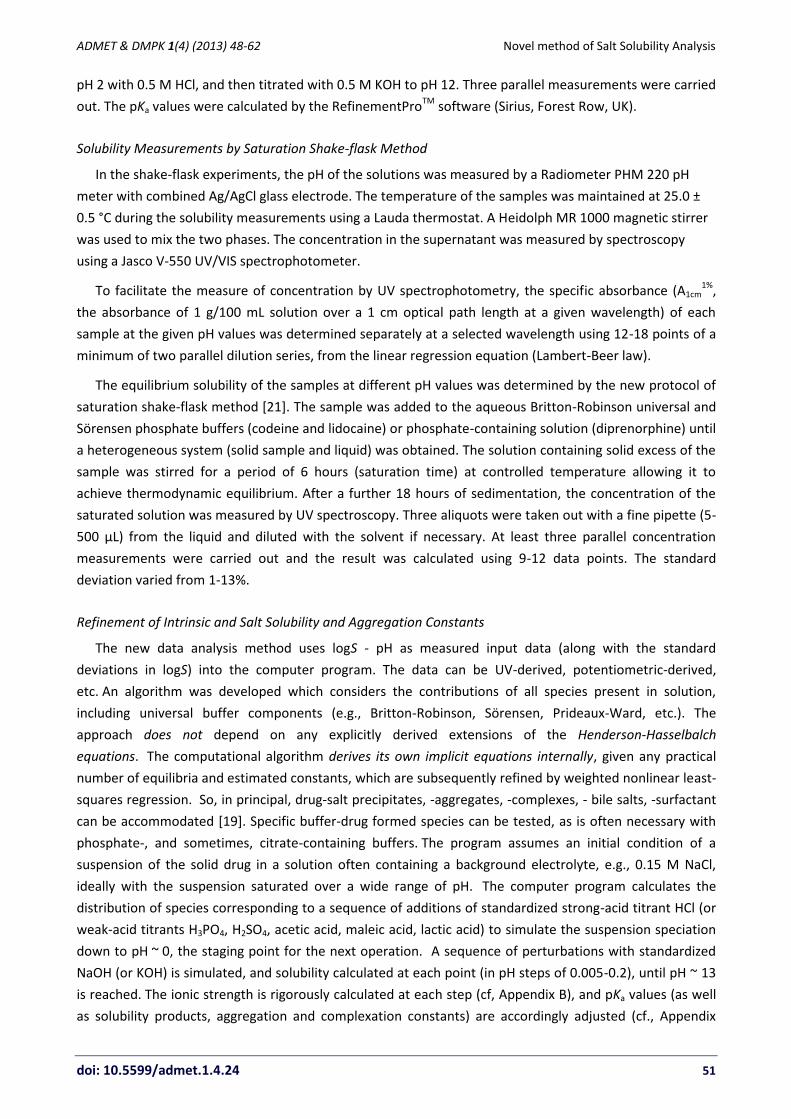
volumes ranged from 0.5 to 15 mL). Table 3 lists the equilibrium constants determined and critical

concentrations (including ionic strength and buffer capacity) calculated in the various assays.

The pKa values of the model compounds are listed in Table 1 at standard state conditions (Iref = 0.15 M,

25 oC), but the primed constants in Table 3 are those that were actually applied at the specific ionic

strength (0.25 – 4.34 M), calculated as described in Appendix B. Those of diprenorphine changed slightly

by 0.0 to +0.05 (pKa1) and 0.0 to -0.04 (pKa2); that of codeine +0.02 to +0.14; that of lidocaine +0.15 to

+0.51. According to the simple Debye-Hückel theory, those of monoprotic bases are expected not to

change, but Eq. B5 predicts otherwise. Also listed in Table 3 are the actual pKsp values used at the particular

ionic strengths, compared to those at Iref.


doi: 10.5599/admet.1.4.24 53

Table 1. Physicochemical properties, 25 °C.

Compound MW log P pKa

Literature

-log S0 = pS0 [M]

Diprenorphine 425.56 3.81a 9.68 ± 0.01

d, 8.52 ± 0.01

d --

Codeine 299.36 1.19b 8.24

b 1.52

e

Lidocaine 234.34 2.44c 7.95

c 2.04

f, 1.88

g, 1.75

h, 1.71

i

a Calculated using ADME Boxes 4.9 (ACD Labs, Toronto).

b[22]

c [23]

d This work.

e[24]

f[16].

g[25]

h[26]

i[27]

The solubility products are also affected significantly when I >> Iref. For example, the phosphate pKsp of

codeine phosphate decreased from 1.00 {1.11} at Iref to -0.07 {0.02} at I = 1.21 {1.07} M, where the braced

value refers to Britton-Robinson universal and the unbraced value refers to Sörensen buffer measurements

(Table 3). Lidocaine showed similar large shifts due to the large I = 4.34 {3.81} M. The changes were much

smaller for the codeine chloride pKsp, since I = 0.33 {0.24} M.

Table 2. Shake-flask solubility data, 25 °Ca

pH Buffer

V (14.85

M H3PO4)

/ml b

V (0.5 M KOH)

/ml b S (mg mL

-1)

Sample Wt.

(g mL-1

)

Expected

Precipitate

0.83 Sör 0.4998 0.0000 4.98 ± 0.04 0.0307 XH2+H2PO4

-(s)

1.94 Sör 0.0111 0.0000 54.1 ± 1.1 0.0601 XH2+Cl

-(s)

3.53 Sör 0.0003 0.0000 45.2 ± 0.9 0.0634 XH2+Cl

-(s)

5.06 Sör 0.0000 0.0082 45.1 ± 1.2 0.0637

XH2+Cl

-(s) +

XH(s)

7.22 Sör 0.0000 0.4969 0.249 ± 0.014 0.0050 XH(s)

8.34 Sör 0.0000 0.5702 0.088 ± 0.021 0.0114 XH(s)

8.83 Sör 0.0000 0.5759 0.032 ± 0.001 0.0007 XH(s)

10.38 Sör 0.0000 0.6251 0.667 ± 0.008 0.0106 XH(s)

11.52 Sör 0.0000 0.8274 4.79 ± 0.11 0.0051 XH(s)

5.00 BR 0.0000 0.1376 52.0 ± 0.1 0.1050 BH+Cl

-(s)

5.00 Sör 0.0000 0.0044 53.0 ± 0.1 0.1535 BH+Cl

-(s)

5.00 BR 0.0000 0.1716 290 ± 38 0.4950 BH+H2PO4

-(s)

5.00 Sör 0.0000 0.0390 308 ± 30 0.5305 BH+H2PO4

-(s)

5.00 BR 0.2149 0.0000 310 ± 15 0.7700 BH+H2PO4

-(s)

5.00 Sör 0.2940 0.0000 294 ± 10 1.0300 BH+H2PO4

-(s)

5.00 BR 0.0000 0.0064 >1000 1.0300 BH+Cl

-(s)

5.00 Sör 0.0000 0.0042 >1000 1.1354 BH+Cl

-(s)

a Sör = Sörensen buffer (0.15 M phosphate, adjusted with NaOH). BR = Britton-Robinson universal buffer

(acetic, phosphoric, and boric acids, each at 0.04 M, adjusted with NaOH to pH 5). b Calculated by pDISOL-X.

The pKa values of the acetate, phosphate, and borate buffer components used were taken from

Wiki-pKa website (<http://www.in-ADME.com/wiki_pka.php/>). These were automatically adjusted for

changes in the ionic strength by pDISOL-X. The changes were most pronounced with phosphoric acid (0.17

– 0.62), and were minimal with acetic and boric acids (0.01-0.06).


54

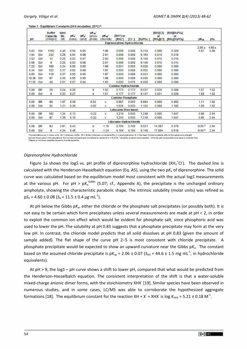
Diprenorphine Hydrochloride

Figure 1a shows the logS vs. pH profile of diprenorphine hydrochloride (XH2+Cl

-). The dashed line is

calculated with the Henderson-Hasselbalch equation (Eq. A5), using the two pKa of diprenorphine. The solid

curve was calculated based on the equilibrium model most consistent with the actual logS measurements

at the various pH. For pH > pKaGIBBS

(5.07; cf., Appendix A), the precipitate is the uncharged ordinary

ampholyte, showing the characteristic parabolic shape. The intrinsic solubility (molar units) was refined as

pS0 = 4.60 ± 0.08 (S0 = 11.5 ± 0.4 µg mL-1

).

At pH below the Gibbs pKa, either the chloride or the phosphate salt precipitates (or possibly both). It is

not easy to be certain which form precipitates unless several measurements are made at pH < 2, in order

to exploit the common ion effect which would be evident for phosphate salt, since phosphoric acid was

used to lower the pH. The solubility at pH 0.83 suggests that a phosphate precipitate may form at the very

low pH. In contrast, the chloride model predicts that all solid dissolves at pH 0.83 (given the amount of

sample added). The flat shape of the curve pH 2–5 is most consistent with chloride precipitate. A

phosphate precipitate would be expected to show an upward curvature near the Gibbs pKa. The constant

based on the assumed chloride precipitate is pKsp = 2.06 ± 0.07 (SXH = 44.6 ± 1.5 mg mL-1

, in hydrochloride

equivalents).

At pH > 9, the logS – pH curve shows a shift to lower pH, compared that what would be predicted from

the Henderson-Hasselbalch equation. The consistent interpretation of the shift is that a water-soluble

mixed-charge anionic dimer forms, with the stoichiometry XHX- [19]. Similar species have been observed in

numerous studies, and in some cases, LC/MS was able to corroborate the hypothesized aggregate

formations [18]. The equilibrium constant for the reaction XH + X- = XHX

- is log KXHX = 5.21 ± 0.18 M

-1.


doi: 10.5599/admet.1.4.24 55

Figure 1. Solubility-pH profiles of the three model drugs studied. (See text)


56

Codeine Hydrochloride and Dihydrogenphosphate

Figure 1b shows the codeine hydrochloride (BH+Cl

-) and phosphate (BH

+H2PO4

-) logS – pH profiles. The

curve was calculated assuming the intrinsic solubility, pS0 = 1.52 (S0 = 12 mg mL-1

, assuming phosphate salt

molecular weight), reported by Kuhne et al. [24]. Although single pH measurements were made, the whole

curve adds useful perspective to the expected solubility – pH relationship. The assignment of the types of

salts formed is possible in the way the assays were designed. The codeine phosphate assay had no source

of chloride, and thus revealed the phosphate pKsp = 1.00 {1.11}. The codeine chloride assay indicated a

significantly higher pKsp = 1.59 {1.57}, suggesting that the salt precipitate was that of the chloride.

Furthermore, the solubility product for the phosphate salt in the case of the chloride was not exceeded

(Table 3), suggesting the absence of phosphate salt in the chloride assay.

Lidocaine Free Base and Hydrochloride

Figure 1c shows the lidocaine phosphate (BH+H2PO4

-) logS – pH profile. The chloride was very soluble

with SBH>1 g mL-1

. The chloride pKsp in Table 3 refer to the minimum possible values: pKspBHCl

= -0.99 {-0.85},

suggesting that the chloride salt is at least 50 times more soluble than the phosphate salt. The solid curve

was calculated assuming the intrinsic solubility, pS0 = 2.04 (S0 = 2.5 mg mL-1

, assuming BH+Cl

- molecular

weight), reported by Bergström et al. [16]. As in the case of the codeine assays, the assignment of the

types of salts formed with lidocaine is possible in the way the assays were designed. The lidocaine free

base assay had no source of chloride, and thus revealed the phosphate pKsp = 0.85 {0.88}. The solubility

product for the phosphate salt in the case of the chloride was not exceeded (Table 3), suggesting the

absence of phosphate salt in the chloride assay.

The unfilled circle symbols in Figure 1c are the solubility values reported by Bergström et al. [16], using

the miniaturized shake-flask method (25 oC, 0.15 M phosphate buffer, 24 h incubation).

Even though the pKsp values of phosphate precipitate in the free base case were nearly identical for the

two buffer systems used, the morphology of the crystals isolated was quite different, as shown in Figure 2,

with the Sörensen buffer producing much larger and better-formed crystals, compared to the Britton-

Robinson buffer (approx. 800 vs. 60 µm, respectively). The X-ray powder diffractograms in Figure 3

confirmed that the crystals formed in the free base assay were those of the same phosphate salt

polymorph.


doi: 10.5599/admet.1.4.24 57

Figure 2. Microphotographs of lidocaine phosphate solids obtained from solubility experiments: (a) Britton-Robinson

buffer, (b) Sörensen buffer.

5 10 15 20 25 30 352Theta (°)

0

500

1000

1500

2000

Inte

ns

ity

(c

ps

)

Figure 3. X-ray powder diffractograms of reference lidocaine base (blue), lidocaine phosphate from solubility

measurement in Britton-Robinson buffer (brown) and in Sörensen buffer (orange).


58

Conclusion

The design of salt solubility assays here and the data analysis capability of the new program, pDISOL-X

offered an opportunity to critically investigate issues related to the challenges of characterizing salt

solubility products, such as the high ionic strengths, which can affect values of equilibrium constants and

the calibration of pH electrodes. The “anomalies” in the shapes of logS – pH profiles that cannot accurately

be predicted by the Henderson-Hasselbalch may be common with sparingly-soluble or practically-insoluble

drugs, such as diprenorphine, but are not always easy to recognize unless accurately-determined pKa values

are available [28]. Phosphate buffers can dramatically influence the solubility profiles of ionizable drugs, as

shown here and elsewhere [16,29]. These and other similar complications may be common, but are not

always easy to interpret quantitatively. In such instances, pDISOL-X may be a helpful data analysis and

simulation tool. It can further aid in the analysis of dissolution mechanisms which depend on the salt

solubility of drugs.

Appendices

A) Explicit Solubility - pH Equations

The idealized relationship between solubility and pH can be readily derived for simple equilibrium models.

The "model" refers to a set of equilibrium equations and the associated equilibrium constants. The

following are examples of such derivations correspond to a diprotic ampholyte.

Precipitation of Diprotic Amphoteric Drug, XH (Henderson-Hasselbalch Equation)

In the case of a diprotic amphoteric drug, a saturated solution can be defined by the equations and the

corresponding constants

XH2+ D H

+ + XH Ka1 = [H

+][XH] / [XH2

+] (A1)

XH D H+ + X

– Ka2 = [H

+][X

–] / [XH] (A2)

HX(s) D XH S0 = [XH] (A3)

Solubility, S, at a particular pH is defined as the mass balance sum of the concentrations of all of the

species dissolved in the aqueous phase:

S = [X–] + [XH] + [XH2

+] (A4)

where the square brackets denote molar concentration of species. The above equation can be

transformed into an expression containing only constants and [H+] (as the only variable), by substituting

the ionization and solubility Eqs. A1-A3 into Eq. A4.

logS = log(Ka1/([XH][H+]) [XH] [H

+] /Ka1 + [XH] + [XH][H

+] / Ka1 )

= log[XH] + log(Ka2 / [H+] + 1 + [H

+] / Ka1 )

= logS0 + log(1 + 10– pKa2+pH

+10+pKa1–pH

) (A5)

Eq. A5 is often called the Henderson-Hasselbalch (HH) equation for a diprotic ampholyte, and describes

a U-shaped logS – pH curve. At the low-pH bend in the logS – pH curve, the pH equals the pKa1; at the other

bend, pH equals the pKa2.

Salt Precipitation of Diprotic Amphoteric Drug, XH


doi: 10.5599/admet.1.4.24 59

Eq. A5 considers only one precipitate, that of the uncharged species XH, defining the “intrinsic

solubility” concentration, S0. If the solubility experiment were carried out as an acid-base (HCl/NaOH)

titration, over a wide range pH <<pKa1 to pH >> pKa2, with enough excess compound added that the

solubility products of the salts XH2+Cl

–(s) and Na

+X

–(s) are exceeded, then the curve would have regions at

low pH and high pH that would not behave as indicated by the HH equation. To describe these processes,

two additional solubility equations need to be added to Eqs. A1-A3:

XH2+Cl

–(s) D XH2

+ + Cl

– Ksp1 = [XH2

+][Cl

–] (A6)

Na+X

–(s) D Na

+ + X

– Ksp2 = [Na

+][X

–] (A7)

Hydrochloride Salt of the Drug, XH2+Cl

–(s)

If enough compound is added to the suspension and the pH is gradually lowered, well below pKa1, at a

critical pH point, called pKa1Gibbs

[30,31], the HH equation is replaced by an approximately horizontal line.

In the salt solubility region, pH < pKa1Gibbs

, Eq. A4 still holds, but [XH2+] becomes constant, instead of

[XH]. Eq. A5 can be modified (using Eqs. A1, A2 and A6) to reflect this.

logS = log(Ka2 Ka1 [XH2+] / [H

+]

2 + Ka1 [XH2

+] / [H

+] + [XH2

+] )

= log[XH2+] + log(1 + 10

–pKa1–pKa2+2pH +10

– pKa1+pH )

= logKsp1 – log[Cl–] + log(1 + 10

–pKa1–pKa2+2pH +10

–pKa1+pH ) (A8)

For pH << pKa1, the right-most logarithmic term in Eq. A8 becomes vanishingly small, and cationic-drug

conditional solubility is described by S(+) = [XH2+] = Ksp1 /[Cl

–]. Eq. A8 largely describes a horizontal line.

However, since the HCl titrant both dilutes the solution and elevates the Cl–, the horizontal line curves

downward for pH < 2, noted as the chloride “common-ion” effect, according to Eq. A8.

Sodium Salt of the Drug, Na+X

–(s)

In the presence of a large excess of compound in alkaline pH >> pKa2, at the second critical pH point,

pKa2Gibbs

, the HH equation is replaced by another approximately horizontal line.

In the salt solubility region, pH > pKa2Gibbs

, Eq. A4 still holds, but [X–] becomes constant, while [XH] and

[XH2+] are variable. Eq. A5 can be further modified (using Eqs. A1, A2 and A7) as

logS = log( [X–] + [X

–][H

+] / Ka2 + [X

–] [H

+]

2 / (Ka1Ka2) )

= log[X-] + log(1 + 10

+ pKa1+pKa2–2pH +10

– pKa2+pH)

= logKsp2 – log[Na+] + log(1 + 10

+ pKa1+pKa2–2pH +10

–pKa2+pH) (A9)

For pH >> pKa2, the right-most logarithmic term in Eq. A9 becomes vanishingly small, and conditional

anionic-drug solubility is described by S(–) = [X–] = Ksp2 / [Na

+]. Since the NaOH titrant both dilutes the

solution and raises the sodium concentration in solution, the horizontal line curves downward for pH > 12,

as a result of the sodium “common-ion” effect, according to Eq. A9.

The Complete Solubility Equation

Across the whole pH range, given enough compound excess, the complete solubility equation consists

of three segments: (a) conditional hydrochloride salt region, pH < pKa1Gibbs

(Eq. A8), (b) drug concentration-

independent “HH” region, pKa2Gibbs

> pH > pKa1Gibbs

(Eq. A5), and (c) conditional sodium salt region, pH >

pKa2Gibbs

(Eq. (A9)).


60

Gibbs pKa Values

At the lower pH = pKa1Gibbs

, two solids co-precipitate: XH2+Cl

–(s) and XH(s). At the higher pH = pKa2

Gibbs,

two different solids co-precipitate: Na+X

–(s) and XH(s). More discussion of the topic may be found in the

literature [19,30,31].

Cationic, Anionic and Neutral Self-Aggregate Formations

In concentrated drug solutions or in solutions containing practically insoluble drugs, oligomeric species,

Xnn–

, (XH2+)n

n+, (XH)n, (XH.X

–)n

n-, (XH.XH2

+)n

n+ , …, can form. These can characteristically alter the shape of the

solubility – pH profile. Consequently, most of Eqs. A1-A9 would need to be modified to accommodate

aggregation equilibria. The resultant solubility equations often become very complex, and not all

combinations of possible species have had the corresponding equations derived. Examples of such

derivations of aggregation-solubility equations may be found in the literature [19].

B) Automatic Ionic Strength Compensation

Generally, the ionic strength, I, changes in the course of an acid-base titration due to ionizations,

additions of titrant, and dilution of concentrations. This change affects acid-base equilibrium constants. In

solubility experiments designed to determine salt solubility products, Ksp, the ionic strength can vary

substantially during a titration, and sometimes reaches values as high as 1 M, or even higher. In contrast,

ionization constants, pKa, are determined at a nearly constant I = 0.15 M, under conditions where low

sample concentrations (e.g., 10-3

to 10-6

M) are “swamped” by the added inert salt (e.g., 0.15 M NaCl or

KCl). The independently-determined pKa constants are critical to the analysis of solubility data, and thus the

above large differences in ionic strength need to be factored in, as described here.

It is a reasonable practice to designate 0.15 M as the “reference” ionic strength, Iref, (“physiological” level)

to which all equilibrium constants are scaled in the solubility assay. In the older literature, the reference

state was often chosen as zero, but in current pharmaceutical applications, 0.15 M is usually chosen, with

no loss of thermodynamic rigor [19].

Since the ionic strength at any given pH point in a titration is likely different from Iref, all ionization

constants need to be locally transformed (from reference Iref to local I) for the calculation of local point

concentrations. The procedure below describes such an adjustment of activity coefficients.

Consider a three-reactant system, based on reactants X, Y and H (proton), whose charges are Qx, Qy, and

+1. The concentration of the jth particular species, Cj, is defined in terms of these reactants

Cj = [XQx

]exj

[YQy

]eyj

[H+]

ehj βj (B1)

associated with the general equilibrium expression

exj X + eyj Y + ehj H D XexjYeyjHehj (B2)

where βj is the cumulative formation constant [19], and exj, eyj, and ehj are the X, Y, and H stoichiometric

coefficients, respectively, of the jth

species.

At each pH point in a solubility assay, I is calculated precisely, according to the general formula

[32]:

I = [NaCl] + [NaOH] + [H+] + ½{Qx(1+Qx) x + Qy(1+Qx) y + Σ Qj(1+Qj) Cj }

+ ½ {│Qx + nX │ - Qx – nX } X + ½ {│Qy + nY │ - Qy – nY )}Y (B3)


doi: 10.5599/admet.1.4.24 61

The last two terms in braces in Eq. B3 take into account any nX or nY number of counter ions introduced to

the solution by drug substances in salt form (per X- or Y-compound, respectively).

The reference set of β(Iref) formation constants are locally transformed to the set β(I) according to

the general expression:

úúû

ù

êêë

é-úúû

ù

êêë

é+

úúû

ù

êêë

é+

úúû

ù

êêë

é+=

)(

)(log

)(

)(log

)(

)(log

)(

)(log)(log)(log

refj

j

refh

hhj

refy

yyj

refx

xxjrefjj

If

If

If

Ife

If

Ife

If

IfeII bb (B4)

where β(I) refers to the ionic strength I, while β(Iref) refers to Iref. The ionic-strength-dependent activity

coefficients of X, Y, H, and jth

species (cf., Eq. B2) are denoted fx, fy, fh, and fj, respectively. A similar

equation was introduced by Avdeef [32], based on the Davies-modified Debye-Hückel equation, which is

reasonably useful up to I = 0.3 M. Since much higher ionic strengths are reached in salt solubility

experiments, Eq. B4 in the current study is cast in an expanded activity coefficient equation based on the

hydration theory proposed by Stokes and Robinson [32,33], further elaborated by Bates et al. [34] and

Robinson and Bates [35] to include single-ion activities, then slightly modified by Bockris and Reddy [36],

and recently applied to solubility data of a drug-like molecule by Wang et al. [7]:

÷÷÷÷

ø

ö

çççç

è

æ

×-+

+

+-+

-=å

å

j

jj

j

j

iiiChC

CC

ahIB

IAQIf

OH

OH

OH )1(loglog

å1)(log

2

2

2i

2 (B5)

The first term on the right side of Eq. B5 is the Debye-Hückel equation accounting for the ion-ion

electrostatic interactions; the second term is related to the decrease in the activity of water due to the

work done in immobilizing some of the bulk water to hydrate ions; the third term is related to free energy

change of the ions, as their concentrations effectively increase when the volume of bulk water decreases

upon hydration of the ions. The parameters at 25°C (molar scale): dielectric constant of water, ε = 78.3,

76.8, 67.3 at I = 0, 0.15, and 1 M (NaCl), respectively [37]; the Debye-Hückel slope, A = 1.825x106 (εT)

-3/2 =

0.512, 0.528, 0.642 at I = 0, 0.15, and 1 M, resp.; B = 50.29 (εT)-1/2

= 0.329, 0.333, 0.355 at I = 0, 0.15, 1 M,

resp.; T is the absolute temperature (K). The two adjustable parameters are åi, corresponding to the mean

diameter of the ith

hydrated ion [38], and hi, the hydration number of the ith

ion [37]. The activity of water,

aH2O = 1.000, 0.995, 0.967 at I = 0, 0.15, 1 M, respectively [36]. CH2O = 55.51 M (concentration of water in

pure solvent form, I = 0). The summation symbols in Eq. B5 are over all charged species (including the

reactants) in the system.

Acknowledgements

We thank Sándor Hosztafi (Semmelweis University, Dept. of Pharmaceutical Chemistry) for the synthesis

of diprenoprhine hydrochloride sample. We also thank Dénes Janke for the XRPD measurements.

References

[1] S. Miyazaki, H. Inouie, T. Nadai, T. Arita, M. Nakano, Chem. Pharm. Bull. 27 (1979) 1441-1447.

[2] S. Miyazaki, M. Oshiba, T. Nadai, J. Pharm. Sci. 70 (1981) 594-596.

[3] B.D. Anderson, R.A. Conradi, J. Pharm. Sci. 74 (1985) 815-820.

[4] B.D. Anderson, K.P. Flora, Preparation of water-soluble compounds through salt formation. In: C.G.

Wermuth (Ed.). The Practice of Medicinal Chemistry. Academic Press, London, 1996, pp. 739-754.

[5] M.T. Ledwidge, O.I. Corrigan, Int. J. Pharm. 174 (1998) 187-200.


62

[6] A.T.M. Serajuddin, M. Pudipeddi, Salt selection strategies, in: Stahl PH, Wermuth CG (Eds.),

Handbook of Pharmaceutical Salts: Properties, Selection, and Use, Wiley-VCH, Weinheim, 2002, pp.

135-160.

[7] Z. Wang, L.S. Burrell, W.J. Lambert, J. Pharm. Sci. 91 (2002) 1445-1455.

[8] P.H. Stahl, Salt selection, in: R. Hilfiker (Ed.), Polymorphism in Pharmaceutical Industry, Wiley-VCH,

Weinheim, 2006, pp. 309-322.

[9] T. Higuchi, M. Gupta, L.W. Busse, J. Amer. Pharm. Assoc. (Sci. Ed.) 42 (1953) 157-161.

[10] T.J. Roseman, S.H. Yalkowsky, J. Pharm. Sci. 62 (1973) 1680-1685.

[11] D.J. Attwood, J. Gibson, J. Pharm. Pharmacol. 30 (1978) 176-180.

[12] A. Fini, G. Fazio, G. Feroci, Int. J. Pharm. 126 (1995) 95-102.

[13] Z. Wang, K.R. Morris, B. Chu, J. Pharm. Sci. 84 (1995) 609-613.

[14] Y. Surakitbanharn, R. McCandless, J.F. Krzyzaniak, R.-M. Dannenfelser, S.H. Yalkowsky, J. Pharm. Sci.

84 (1995) 720-723.

[15] W.H. Streng, D.H.-S. Yu, C. Zhu, Int. J. Pharm. 135 (1996) 43-52.

[16] C.A.S. Bergström, K. Luthman, P. Artursson, Eur. J. Pharm. Sci. 22 (2004) 387-398.

[17] A. Avdeef, Adv. Drug Deliv. Rev. 59 (2007) 568-590.

[18] E. Shoghi, E. Fuguet, E. Bosch, C. Ràfols, Eur. J. Pharm. Sci. 48 (2013) 291-300.

[19] A. Avdeef, Absorption and Drug Development, Second Edition. Wiley-Interscience, Hoboken, NJ,

2012.

[20] A. Avdeef, J.J. Bucher, Anal. Chem. 50 (1978) 2137-2142.

[21] E. Baka, J. Comer, K. Takács-Novák, J. Pharm. Biomed. Anal. 46 (2008) 335-341.

[22] A. Avdeef, D.A. Barrett, P.N. Shaw, R.D. Knaggs, S.S. Davis, J. Med. Chem. 39 (1996) 4377-4381.

[23] A. Avdeef, K.J. Box, J.E.A. Comer, C. Hibbert, K.Y. Tam, Pharm. Res. 15 (1997) 208-214.

[24] R. Kuhne, R-U. Ebert, F. Kleint, G. Schmidt, G. Schuurmann, Chemosphere 30 (1995) 2061-2077.

[25] E. Shoghi, E. Fuguet, C. Ràfols, E. Bosch, Chem. Biodivers. 6 (2009) 1789-1795.

[26] C.M. Wassvik, A.G. Holmén, R. Draheim, P. Artursson. LogP-independent solubility of drugs -

molecular descriptors for solid-state limited solubility. In: C.M. Wassvik. PhD Thesis, Univ. Uppsala,

2006.

[27] S. Pinsuwan, P.B. Myrdal, Y.-C. Lee, S.H. Yalkowsky, Chemosphere 35 (1997) 2503-2513.

[28] G. Völgyi, E. Baka, K. Box, J. Comer, K. Takács-Novák, Anal. Chim. Acta 673 (2010) 40-46.

[29] W.H. Streng, S.K. Hsi, P.E. Helms, H.G.H. Tan, J. Pharm. Sci. 73 (1984) 1679-1684.

[30] A. Avdeef, Pharm. Pharmacol. Commun. 4 (1998) 165-178.

[31] W.H. Streng, Int. J. Pharm. 186 (1999) 137–140.

[32] A. Avdeef, J. Pharm. Sci. 82 (1993) 183-190.

[33] R.H. Stokes, R.A. Robinson, J. Amer. Chem. Soc. 70 (1948) 1870-1878.

[34] R.G. Bates, B.R. Staples, R.A. Robinson, Anal. Chem. 42 (1970) 867-871.

[35] R.A. Robinson, R.G. Bates, Marine Chem. 6 (1978) 327-333.

[36] J.O’M. Bockris, A.K.N. Reddy, Modern Electrochemistry, Vol. 1. Plenum Publishing Corp., New York,

NY, 1973.

[37] R.A. Robinson, R.H. Stokes, Electrolytic Solutions. 2nd

Revised Ed. Dover Publications, Inc., Mineola,

NY, 2002.

[38] J. Kielland, J. Amer. Chem. Soc. 59 (1937)1675-1678.

©2013 by the authors; licensee IAPC, Zagreb, Croatia. This article is an open-access article distributed under the terms and

conditions of the Creative Commons Attribution license (http://creativecommons.org/licenses/by/3.0/)

Salt Solubility Products of Diprenorphine Hydrochloride ... · Salt Solubility Products of...

Documents

Transcript of Salt Solubility Products of Diprenorphine Hydrochloride ... · Salt Solubility Products of...