
Salt Brine Blending to Optimize Deicing and Anti-Icing...
115
Salt Brine Blending to Optimize Deicing and Anti-Icing Performance and Cost Effectiveness, Phase II Stephen J. Druschel, Principal Investigator Center for Transportation Research and Implementation Minnesota State University, Mankato December 2014 Research Project Final Report 2014-43
Transcript of Salt Brine Blending to Optimize Deicing and Anti-Icing...

Salt Brine Blending to Optimize Deicing and
Anti-Icing Performance and Cost Effectiveness, Phase II
Stephen J. Druschel, Principal Investigator Center for Transportation Research and Implementation
Minnesota State University, Mankato
December 2014
Research ProjectFinal Report 2014-43

To request this document in an alternative format call 651-366-4718 or 1-800-657-3774 (Greater Minnesota) or email your request to [email protected]. Please request at least one week in advance.
Technical Report Documentation Page 1. Report No. 2. 3. Recipients Accession No. MN/RC 2014-43 4. Title and Subtitle 5. Report Date Salt Brine Blending to Optimize Deicing and Anti-Icing Performance and Cost Effectiveness, Phase II
December 2014 6.
7. Author(s) 8. Performing Organization Report No. Stephen J. Druschel,
9. Performing Organization Name and Address 10. Project/Task/Work Unit No. Center for Transportation Research and Implementation 342 Trafton North Minnesota State University Mankato, MN 56001
11. Contract (C) or Grant (G) No.
(C) 02829
12. Sponsoring Organization Name and Address 13. Type of Report and Period Covered Minnesota Department of Transportation Research Services & Library 395 John Ireland Boulevard, MS 330 St. Paul, Minnesota 55155-1899
Final Report 14. Sponsoring Agency Code
15. Supplementary Notes http://www.lrrb.org/pdf/201443.pdf http://www.lrrb.org/pdf/201443A.pdf 16. Abstract (Limit: 250 words)
This report presents the evaluation of winter maintenance efforts, including applications of deicers and anti icers and plowing, in parallel conditions on actual pavements to assess intuitions based on observations and anecdotal evidence. Parallel conditions eliminate the issue of test sections being in slightly different geographies. Four different aspects were evaluated in this effort:
• Anti icer persistence, measured in response to actual traffic through drainage off defined roadway sections of an elevated highway;
• Deicer effectiveness, techniques and materials evaluated at two proximal facilities across six and three parallel treatment lanes of 1,000 feet length;
• Plow effectiveness, techniques and equipment evaluated at the same locations as the deicer effectiveness evaluation; and,
• Pavement study of anti icer persistence in response to precipitation, performed using asphalt and Portland cement concrete pavements in a laboratory setting.
Results of this work indicate factor interaction such as truck traffic plus deicer use or roadway crosswind and deicer distribution may have significant impact on differences in winter maintenance performance and deicer efficiency.
17. Document Analysis/Descriptors 18. Availability Statement Deicers, Anti-icing, Snowplows, Winter maintenance, Snow and ice control, Pavements, Traffic
No restrictions. Document available from: National Technical Information Services, Alexandria, Virginia 22312
19. Security Class (this report) 20. Security Class (this page) 21. No. of Pages 22. Price Unclassified Unclassified 115

Salt Brine Blending to Optimize Deicing and Anti-Icing Performance and Cost Effectiveness, Phase II
Final Report
Prepared by:
Stephen J. Druschel Center for Transportation Research and Implementation
Minnesota State University, Mankato
December 2014
Published by: Minnesota Department of Transportation
Research Services & Library 395 Ireland Boulevard, MS 330
St. Paul, MN 55155
This report represents the results of research conducted by the author and does not necessarily represent the views or policies of the Minnesota Department of Transportation or Minnesota State University, Mankato. This report does not contain a standard of specified technique. The Minnesota Department of Transportation and Minnesota State University, Mankato do not endorse products or manufacturers. Any trade or manufacturers’ names that may appear herein do so solely because they are considered essential to this report.

Acknowledgments
This report would not be possible without the support of the professionals at the Minnesota Department of Transportation (MnDOT). Many district personnel plowed, salted, drove or shared information in support of this project. Their support greatly increased the quality of this report and the applicability of the results to the wide range of Minnesota conditions. MnDOT also provided plow truck and payloader equipment, deicer chemicals, safety training and meeting space, all substantial ingredients to our recipe for success. Carver County provided a truckload of magnesium chloride-treated rock salt for deicer testing, and although it was unable to be incorporated into the field study, the county’s support was helpful.
Canterbury Park and Valleyfair provided large pavement areas for plowing and deicing evaluations. Their flexibility, support and overall contribution to this effort is warmly appreciated.
Student workers from the Civil Engineering program at Minnesota State University, Mankato, contributed substantial effort in support of this project, including Danielle Alinea, Anthony Adderley, Meghann Chiodo, Thu Hoang Anh (Amy) Nguyen and Andy Pfeffer. Thanks to all of these students for their hours and hours of preparation, field work, literature search, lab testing and data analysis. Researchers on this project would also like to thank Karnell Johnson of the Center for Transportation Research and Implementation for assistance with administrative services.
This project was funded by the Minnesota Department of Transportation through agreement 02829. MnDOT’s support is gratefully acknowledged.

Table of Contents
Chapter 1: Introduction ................................................................................................................... 1
1.1: History of Roadway Deicing ............................................................................................... 2
1.2: Previous Studies of Deicing and Anti-Icing Performance .................................................. 3
Chapter 2: Anti-Icing Persistence Study ........................................................................................ 8
2.1: Test Method ......................................................................................................................... 8
2.1.1: Method design ............................................................................................................... 8
2.1.2: Field Site ....................................................................................................................... 9
2.1.3: Drainage Measurement ............................................................................................... 18
2.1.4: Weather Measurement ................................................................................................. 22
2.1.5: Cameras and Photography .......................................................................................... 23
2.1.6: Plow and Deicer Spreading Operations ..................................................................... 23
2.2: Results ................................................................................................................................ 26
2.3: Evaluation .......................................................................................................................... 29
2.3.1: Comparison of Chloride Mass Flow Rates and Cumulative Weekly Amounts ........... 30
2.3.2: Comparison of Traffic Effects by Storm Event ............................................................ 33
2.4: Conclusions and Recommendations .................................................................................. 35
Chapter 3: Deicer Effectiveness Study ........................................................................................ 36
3.1: Test Method ...................................................................................................................... 36
3.1.1: Method Design ............................................................................................................ 36
3.1.2: Field Sites .................................................................................................................... 37
3.1.3: Weather Measurement ................................................................................................. 43
3.1.4: Cameras and Photography .......................................................................................... 43
3.1.5: Plow and Deicer Spreading Operations ..................................................................... 45
3.2: Results ................................................................................................................................ 48
3.3.1: Effect of Time and Temperature .................................................................................. 54
3.3.2: Effect of Snow Structure .............................................................................................. 55
3.3.3: Effect of Deicer Application Rate................................................................................ 55
3.3.4: Effect of Traffic............................................................................................................ 57
3.3.5: Effect of Prewet ........................................................................................................... 58

3.3.6: Effect of Wind and Sun or Overcast ............................................................................ 63
3.4: Conclusions ........................................................................................................................ 63
Chapter 4: Plow Effectiveness Study ........................................................................................... 65
4.1: Test Method ....................................................................................................................... 65
4.1.1: Method Design ............................................................................................................ 65
4.1.2: Field Sites .................................................................................................................... 65
4.1.3: Weather Measurement ................................................................................................. 71
4.1.4: Cameras and Photography .......................................................................................... 71
4.1.5: Plow and Deicer Spreading Operations ..................................................................... 74
4.2: Results ................................................................................................................................ 75
4.3: Evaluation .......................................................................................................................... 78
4.3.1: Comparison of Plow Scrape Quality Across Single Site ............................................. 79
4.3.2: Comparison of Plow Scrape Quality Across Single Site ............................................. 82
4.3.3: Evaluation of Plow Speed Effects on Dislodged Snow Removal ............................... 82
4.4: Conclusions ........................................................................................................................ 88
Chapter 5: Pavement Study .......................................................................................................... 89
5.1: Test Method ....................................................................................................................... 92
5.1.1: Method design ............................................................................................................. 92
5.1.2: Pavement Samples ....................................................................................................... 92
5.1.3: Deicers ......................................................................................................................... 93
5.1.4: Precipitation and Drainage ........................................................................................ 93
5.2: Results ................................................................................................................................ 96
5.3: Evaluation .......................................................................................................................... 96
5.4: Conclusions and Recommendations .................................................................................. 97
Chapter 6: Conclusions ................................................................................................................ 99
References ................................................................................................................................... 101
Appendix A: Calibration of Flow Measurement Weirs
Appendix B: Calibration of Leveloggers for Conductivity and Salt Brine Concentration
Appendix C: Weather Data of Field Days and Field Season
Appendix D: Temperature, Conductivity and Water Depth Results
Appendix E: Mass Flow and Cumulative Mass Flow Calculation Results

Appendix F: Weather Data of Field Days and Field Season
Appendix G: Time-Lapse Photographs of Lane Treatments
Appendix H: Salt Evaluation by Rate at 25° F
Appendix I: Salt Evaluation by Rate at 4° F
Appendix J: Traffic Effect Evaluation
Appendix K: Photographs of Lane Plowing with Snow Conditions Before and After Plowing
Appendix L: Drainage Results
List of Figures
Figure 1. Winter conditions conducive to ice buildup on roadways …………………………….9
Figure 2. Deicer and anti icer application equipment………………………………………...…11
Figure 3. North Star Bridge, US 169 over the Minnesota River at Mankato, Minnesota…….....12
Figure 4. North Star Bridge drainage..…………………………………………... ……………..13
Figure 5. North Star Bridge plan showing drainage inlet locations…………………………..…15
Figure 6. Traffic on the North Star Bridge………………..…………………………………….18
Figure 7. Flow-through cells…………………………………………………..………………...21
Figure 8. Calibration of flow measurement in weirs of plastic drum…..……………………….22
Figure 9. Calibration of conductivity measurement in data loggers.………….. ……………….22
Figure 10. Debris clog at Location A, March 27, 2014….……………………………………...23
Figure 11. Ice blocking……………………………………...…………………………………..25
Figure 12. Blocked down chute at Location H.…………………………………………………31
Figure 13. Pavement areas with snow cover prior to plowing………………………………..….38
Figure 14. Pavement discontinuities, noted prior to snowfall………………………………...…40
Figure 15. First snowplow cuts……………………………………………………………….…40
Figure 16. Placement of lane marking flags and stationing of lane distance……………………41
Figure 17. Completed lanes.……………………………………………………………………..42
Figure 18. Comparison of conditions possible between field sites………………………………43
Figure 19. Exploration of techniques to create ice sheet patches on pavement lanes………...…44
Figure 20. Weather monitoring tools.……………………………………………………………45
Figure 21. Time-lapse cameras and a resulting photograph.…………………………………….46
Figure 22. Plow and deicer equipment on a MnDOT truck used for this study……………...…47

Figure 23. MnDOT truck spreading deicer off left rear while moving forward with a right-angled front plow……………………………………………………………………………………...…48
Figure 24. Pavement areas with snow cover prior to plowing……………….………………….66
Figure 25. Pavement discontinuities, noted prior to snowfall.……………………………….....67
Figure 26. First snowplow cuts.…………………………………………………………………68
Figure 27. Placement of lane marking flags and stationing of lane distance….…...……………68
Figure 28. Comparison of conditions possible between field sites…...…………………………69
Figure 29. Completed lanes…………………………………………………………………..…70
Figure 30. Weather monitoring tools……………………………………………………………71
Figure 31. Time-lapse cameras and a resulting photograph…………………………………….73
Figure 32. Plow and deicer equipment on a MnDOT truck used for this study………………...74
Figure 33. MnDOT truck spreading deicer off left rear while moving forward with a right-angled front plow………………………………………………………………………………...75
Figure 34. Typical time lapse photograph showing front and wing plowing plus deicer application (left rear distributor).………………………………………………………………...78
Figure 35. Time-lapse photographs from immediately (~1 minute) after plowing …………….80
Figure 36. Time-lapse photographs from immediately (~1 minute) after plowing (except CD 1 and CD 2 are from 11 and 6 minutes after plowing, respectively)…………………………...….81
Figure 37. Comparison between Canterbury Park (CD Lanes) and Valleyfair (VF Lanes) sites using time-lapse photographs from immediately (~1 minute) after plowing.…………………...84
Figure 38. Comparison between Canterbury Park (CD Lanes) and Valleyfair (VF Lanes) sites using time-lapse photographs from immediately (~1 minute) after plowing (except CD 1 and VF3 are from 11 and 6 minutes after plowing, respectively)………………………………...….85
Figure 39. Comparison between different plowing speeds within similar snow and weather conditions of a single site on a single day…………………………………………………….….86
Figure 40. Comparison of plowing on different speeds during different snow and weather conditions of two lanes from a single site on different days.…………………………………….87
Figure 41. Winter conditions conducive to ice buildup on roadways…………………………...90

Figure 42. Deicer and anti icer application equipment………………………………………….91
Figure 43. Pavement specimen collection, CSAH 17 project…………………………………...94
Figure 44. Anti icer application to defined pavement area……………………………………...95
Figure 45. Precipitation water application (left) and drainage collection (right)…………….…95

List of Tables
Table 1. Storm drainage locations used in measurements.………………………………...……16
Table 2. Events and flow measurements pertaining to North Star Bridge locations.…………...28
Table 3. Replicate evaluation……………………………………………………………………29
Table 4. Magnitude of highest chloride mass flow rates in pounds per lane mile per minute, given by location and week of observation……………………………...…………………..…...32
Table 5. Magnitude of cumulative chloride mass flow rates in pounds per lane mile per week, given by location and week of observation.……………………………………...………………33
Table 6. Comparison of cumulative chloride mass magnitude and timing by traffic conditions for specific storm events..………………………………………………………………………..34
Table 7. Deicing activities by date and weather conditions.…………………………………….49
Table 8. Deicing activities by lane for 1/29/2014, at 25°F, clear and sunny, with wind 5-15 mph……………………………………………………………………………………………....50
Table 9. Deicing activities by lane for 2/6/2014, at 4°F, clear and sunny, with wind 8-12 mph………………………………………………………………………………………………51
Table 10. Deicing activities by lane for 2/14/2014, at 13°F, clear and sunny, with wind 8-12 mph..……………………………………………………………………………………..………52
Table 11. Deicing activities by lane for 2/19/2014, at 40°F, clear and sunny, with wind 0-3 mph.……………………………………………………………………………………………...53
Table 12. Ice melt capacity for rock salt (from Druschel, 2012)………………………………..54
Table 13. Comparison of prewet and no prewet for different traffic conditions at an air temperature of 4° F with a deicer application rate of 400 pounds per lane mile.………………..59
Table 14. Comparison of prewet and no prewet for different traffic conditions at an air temperature of 25° F with a deicer application rate of 400 pounds per lane mile..……………...60
Table 15. Comparison of prewet and no prewet for different traffic conditions at an air temperature of 13° F with a deicer application rate of 800 pounds per lane mile. ………...……61
Table 16. Comparison of prewet and no prewet for different traffic conditions at an air temperature of 40°F with a deicer application rate of 800 pounds per lane mile………………..62
Table 17. Plowing activities by date, weather and snow conditions……………………………76
Table 18. Deicers considered in this study, listed with active components as listed by the vendor……………………………………………………………………………………………93
Executive Summary
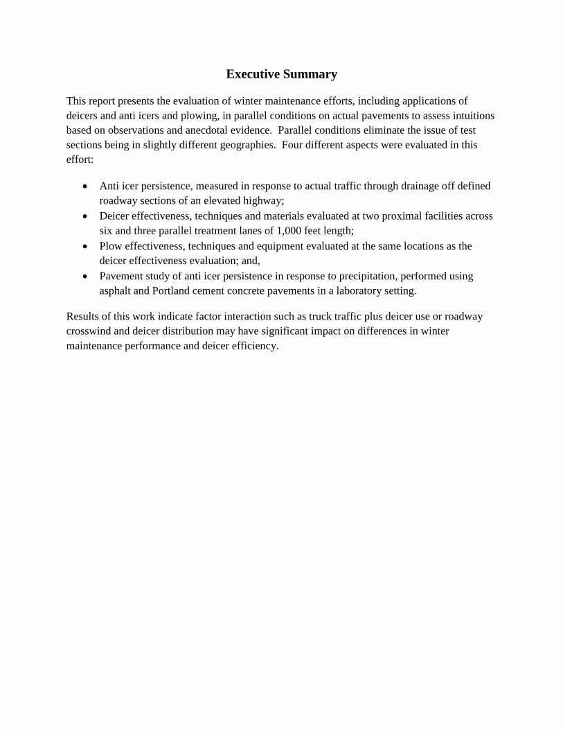
This report presents the evaluation of winter maintenance efforts, including applications of deicers and anti icers and plowing, in parallel conditions on actual pavements to assess intuitions based on observations and anecdotal evidence. Parallel conditions eliminate the issue of test sections being in slightly different geographies. Four different aspects were evaluated in this effort:
• Anti icer persistence, measured in response to actual traffic through drainage off defined roadway sections of an elevated highway;
• Deicer effectiveness, techniques and materials evaluated at two proximal facilities across six and three parallel treatment lanes of 1,000 feet length;
• Plow effectiveness, techniques and equipment evaluated at the same locations as the deicer effectiveness evaluation; and,
• Pavement study of anti icer persistence in response to precipitation, performed using asphalt and Portland cement concrete pavements in a laboratory setting.
Results of this work indicate factor interaction such as truck traffic plus deicer use or roadway crosswind and deicer distribution may have significant impact on differences in winter maintenance performance and deicer efficiency.
1
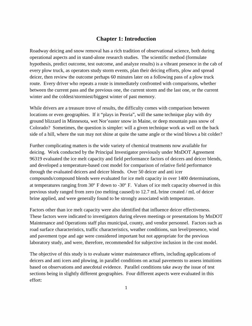
Chapter 1: Introduction
Roadway deicing and snow removal has a rich tradition of observational science, both during operational aspects and in stand-alone research studies. The scientific method (formulate hypothesis, predict outcome, test outcome, and analyze results) is a vibrant presence in the cab of every plow truck, as operators study storm events, plan their deicing efforts, plow and spread deicer, then review the outcome perhaps 60 minutes later on a following pass of a plow truck route. Every driver who repeats a route is immediately confronted with comparisons, whether between the current pass and the previous one, the current storm and the last one, or the current winter and the coldest/stormiest/biggest winter of past memory.
While drivers are a treasure trove of results, the difficulty comes with comparison between locations or even geographies. If it “plays in Peoria”, will the same technique play with dry ground blizzard in Minnesota, wet Nor’easter snow in Maine, or deep mountain pass snow of Colorado? Sometimes, the question is simpler: will a given technique work as well on the back side of a hill, where the sun may not shine at quite the same angle or the wind blows a bit colder?
Further complicating matters is the wide variety of chemical treatments now available for deicing. Work conducted by the Principal Investigator previously under MnDOT Agreement 96319 evaluated the ice melt capacity and field performance factors of deicers and deicer blends, and developed a temperature-based cost model for comparison of relative field performance through the evaluated deicers and deicer blends. Over 50 deicer and anti icer compounds/compound blends were evaluated for ice melt capacity in over 1400 determinations, at temperatures ranging from 30° F down to -30° F. Values of ice melt capacity observed in this previous study ranged from zero (no melting caused) to 12.7 mL brine created / mL of deicer brine applied, and were generally found to be strongly associated with temperature.
Factors other than ice melt capacity were also identified that influence deicer effectiveness. These factors were indicated to investigators during eleven meetings or presentations by MnDOT Maintenance and Operations staff plus municipal, county, and vendor personnel. Factors such as road surface characteristics, traffic characteristics, weather conditions, sun level/presence, wind and pavement type and age were considered important but not appropriate for the previous laboratory study, and were, therefore, recommended for subjective inclusion in the cost model.
The objective of this study is to evaluate winter maintenance efforts, including applications of deicers and anti icers and plowing, in parallel conditions on actual pavements to assess intuitions based on observations and anecdotal evidence. Parallel conditions take away the issue of test sections being in slightly different geographies. Four different aspects were evaluated in this effort:

2
• Anti icer persistence, measured in response to actual traffic through drainage off defined roadway sections of an elevated highway;
• Deicer effectiveness, techniques and materials evaluated at two proximal facilities across six and three parallel treatment lanes of 1000 feet length;
• Plow effectiveness, techniques and equipment evaluated at the same locations as the deicer effectiveness evaluation; and,
• Pavement study of anti icer persistence in response to precipitation, performed using asphalt and Portland cement concrete pavements in a laboratory setting.
Each effort contributes to identification of best practices for winter maintenance. Whether MnDOT, city or county personnel, or private contractor, winter deicing is a high intensity, high cost effort that can surely use greater characterization of performance benefits of available deicer and anti icer products for use in predicting efforts required for expected driver level of service.
1.1: History of Roadway Deicing
Clearing snow from roadways is an effort as old as roadways themselves, at least in cold climates. Truck mounted plows came into wide use by the 1920’s. Abrasives such as sand, coal bottom ash or clinker were used to increase friction on icy roadways, once plowed. During the winter of 1941-42, New Hampshire became the first state to establish a systematic use of salt for deicing (TRB Special Report 235, 1991). About 1 million tons per year of salt were used for deicing in 1950; by 1970, 10 million tons per year were being used, an amount that has remained consistent though adjusted by winter-to-winter variation (USGS, 2014). The rapid increase of salt usage from 1950-1970 coincides with the rise of driver expectation for bare pavements during winter conditions, excepting storm events (TRB Special Report 235, 1991).
Distribution of deicer on roadways has progressed from basic to quite advanced techniques (TRB Special Report 235, 1991, and author observation):
• 1940’s: stationing of a shoveler in the back of a dump truck; • 1950’s: installation of a spinner plate below gravity fed chute for full roadway broadcast; • 1970’s: distribution through a smaller spinner plate or line drop onto high side of travel
lane, to encourage undercutting of ice through brine drainage; • 1980’s: incorporation of pre-wetting treatment on to granular deicer to improve roadway
adherence and resistance to bounce or blow off; • 1990’s: introduction of pre-storm chemical treatment of pavements to anti ice;

3
• 2000’s: matching deicer spreading technologies with “smart vehicle” techniques such as Maintenance Decision Support System (MDSS), Automated Vehicle Location (AVL) and Road Weather Information Systems (RWIS); and,
• 2010’s: introduction of brine blending systems and multi-component liquid chemical systems.
Deicing material selection has been a consideration constant since the introduction of deicing as a technique, as cost-benefit analyses have accompanied the use of rock salt (bulk mined sodium chloride), solar salt (evaporated remains of solution mined or sea water originated salt), magnesium chloride, calcium chloride, acetates, alcohols, carbohydrates and any other product available in bulk that can reduce the freeze point of water.
1.2: Previous Studies of Deicing and Anti-Icing Performance
Evaluations of deicing and anti-icing performance occur with every winter storm event, with every driver on a given roadway impacted by snow or ice. Given the difficulty of driving in winter conditions, it is no wonder this anecdotal evaluation occurs. However, formal studies of performance in the technical literature are few, particularly studies with evaluations of factors rather than comparisons of procedures.
Chollar (1988) summarizes field studies done during the winter of 1986 – 87 comparing the performance of calcium magnesium acetate (CMA) and rock salt at four locations: Wisconsin, Massachusetts, Ontario and California. CMA was found to deicer slower than rock salt although eventually reached a similar performance level. CMA was also found to have roadway distribution and persistence issues caused by lower density particles: (1) particles would spread farther than rock salt (ending off the vehicle lane); and (2) were more susceptible to wind erosion from the roadway. Operational issues were also identified with CMA, including distributor clogging due to material softening with moisture absorbance and increased adherence to vehicle windshields.
Sypher:Mueller (1988) describe field trials of CMA and sodium formate (NaFo) against the performance of sodium chloride done during the winter of 1987 – 88 in Ottawa, Ontario. The purpose of this study was to assess deicer alternatives that were associated with lower environmental, vegetation and corrosion damage than with sodium chloride. Test sections were designated for the application treatments plus a no-application control using two parallel roadways: a two-lane, low volume, low speed city road; and a four lane, high volume, moderate speed regional road (traffic amounts were not provided). This study was the first to use friction testing as a measure of deicer performance. Slower melt times for both alternative deicers and

4
higher application rate needed for equivalent performance of CMA were noted. Cost increases of 33 and 13 times the cost of sodium chloride were noted for CMA and NaFo, respectively.
Raukola, et al (1993) described an anti-icing program evaluation in Finland that used a residual chloride measurement to assess anti-icing persistence on pavement in a medium duty roadway with 6100 average daily traffic. Anti-icing was applied in liquid form only for this study. Decreases in surface chloride concentration were found to be associated with roadway moisture most of all. Other factors positively correlated to a decline in surface chloride concentration included traffic, initial application amount, and applicator speed. No difference in the pattern of persistence was noted between sodium chloride and calcium chloride.
Manning and Perchanok (1993) evaluated the use of CMA at two locations in Ontario using a comparison with rock salt for performance measures. The two locations differed greatly in the temperature, precipitation and traffic conditions. Four different winter periods were used from 1986 – 87 to 1990 – 91. With heavy traffic and light snow, CMA was generally equivalent to rock salt, although 20 – 70% more CMA was applied in an attempt to match the ionic characteristics of rock salt. Both light traffic and heavy snow conditions caused decreases in performance of CMA relative to rock salt.
Stotterud and Reitan (1993) discussed the findings of an anti-icing evaluation in Norway that considered weather factors on ice prevention. Performance was assessed by friction measurements. Anti-icing was negatively affected by snow intensity, lower temperatures and the occurrence of freezing rain. Duration (persistence) of anti-icing materials was found to be reduced by increases in traffic or surface moisture, either as frost or drizzle. Persistence could be as long as 2 – 3 days on the tested roadway, if low temperatures and low humidity occurred prior to the storm event. Pavement type and age were discussed as factors in performance, but no clear trend was identified only differences discussed.
Woodham (1994) describes a testing program that used a single storm event in 1991 with twelve roadway sections of 1/10th mile each in a single community in Colorado. Four different material preparations were evaluated: (1) magnesium chloride and sand; (2) calcium chloride and sand; (3) sodium chloride (rock salt) and sand; and (4) magnesium chloride, sodium chloride and sand. Salt of any type was limited to 80 pounds per lane mile due to societal constraints. Sand component amount was varied in the blends, as an objective of the study was to find a lower amount of sand in a blend that would achieve expected performance or better. Prewetting was also evaluated and found to greatly improve deicing time. Magnesium chloride – sand and sodium chloride – sand mixtures were found to perform best.
Blackburn, et al (1994) presented a large and comprehensive study of anti-icing, consisting of liquid, solid and prewet solid anti-icing materials and techniques tested at fourteen locations in

5
nine states (CA, CO, MD, MN, MO, NV, NY, OH and WA) during the winters of 1991 – 92 and 1992 – 93. Materials and techniques were tested against control sections where conventional snow and ice control practices of the particular state were used. Friction testing and chloride residual testing were used for performance measurement, and results were presented along with weather, pavement condition and air temperature records. State departments of transportation were the testing agencies, and training materials were developed within the study for anti-icing techniques, testing methods and quality control procedures. Difficulties encountered included the lack of equipment available for prewetting, equipment targeted for the low treatment levels associated with anti-icing, and a lack of vendor testing of operational characteristics of spreading equipment.
Findings of Blackburn, et al (1994) included a mixed outcome about the reduction of overall salt use, as some locations experienced increases in salt use and some locations first decreased then increased salt use. Salt use outcome variations were attributed to the contrasts of winter storm patterns between the two years. Overall, anti-icing at 100 pounds per lane mile with liquid or prewetted solid was found to greatly improve roadway operation during winter conditions when temperatures were above 20° F; dry solids were found to have persistence on the roadway inadequate for effective anti-icing due to blow off or traffic effects. Prewet rates of 5 – 6 gal/ton and 10 – 12 gal/ton were found minimal but effective for prewetting on the spinner and in the truck bed, respectively, although recommendation was given to increase the rate by 50% for greater effectiveness and reliability of method. Magnesium chloride was evaluated and found to be an effective anti-icing material as a liquid or prewet on sodium chloride. Anti-icing techniques were found to be ineffective or even detrimental if used during freezing rain or drizzle events, or on compacted snow.
Blackburn, et al (1993) presented preliminary observations of techniques and the overall program later presented Blackburn, et al (1994).
Ketcham, et al (1998) produced a follow on study to Blackburn, et al (1994) using eight of the sites previously studied and adding eight new sites. Fifteen states were involved in the study (IA, KS, MA, NH, OR and WI were added), although results were only reported from twelve sites in eleven states addressing ADTs of 3000 – 40,000. The goal of this study, similar to the previous study, was to evaluate new techniques of anti-icing in comparison with conventional practices of the particular state, with the objective to further encourage development and implementation of the new anti-icing practices. As before, performance was measured with friction tests and pavement observations, while perceptions of passenger vehicle handling after treatment was added. Results were graphed across the storm times then evaluated with statistical evaluations of friction values by pavement conditions and treatment approach (either conventional or anti-icing based). Two to fourteen storms per year were evaluated for each site. A wide range of treatment

6
materials were evaluated including rock salt, fine salt, calcium chloride, magnesium chloride, potassium acetate, and abrasives.
In the study by Ketcham, et al (1998), friction was found to be reduced by lower air temperatures (greatest effect), higher precipitation rates and decreasing traffic volume (least effect). Snowfall intensity was also particularly identified, as packed snow was observed to occur after an upturn in intensity, although the results were not quantified. Friction was consistently worse with “snow” conditions than with “light snow” conditions. Cost analyses of five highway sections were inconclusive, as anti-icing techniques resulted in both lower and higher costs. Reasons for the costs to increase included higher priced chemicals being used, test operations not being completely typical, and anti-icing not being “tuned” to achieve the full potential of ice prevention and removal. Additionally, clean up of abrasives (when used) was identified as a significant cost.
Anti-icing performance factors identified by Ketcham, et al (1998) as needing further evaluation included:
• Lower levels of service being incorporated as a flexible storm response; • Rural versus urban roadway treatments; • Abrasives as a complementary strategy to anti-icing; • The effective application of solids and prewet solids for anti-icing; • Persistence of anti-icing treatments between storms; • The optimum timing of anti-icing treatments ahead of storms; • Interaction of anti-icing with open graded pavement courses; and, • Effective anti-icing techniques for freezing rain conditions.
Highway Innovative Technology Evaluation Center (1999) presents an evaluation of applications and techniques using Ice Ban Magic liquid deicer product. Seven state highway agencies (AK, CO, IN, NE, NY, WA and WI) and one county were involved. Performance advantages were observed in comparison to magnesium chloride at low temperatures and with residual material lasting from one storm to the next. Advantages over sodium chloride brine were also observed when used as either a prewet or stockpile treatment. However, Ice Ban was found to be particularly susceptible to occurrences of refreeze and freezing rain, in that lower effectiveness than traditional materials was observed under these conditions.
Two laboratory studies have particular applicability to this project. Trost, et al (1987) described deicing as fundamentally controlled by undercutting, allowing traffic to break up delaminated ice. Undercutting was further described as a two-phased behavior, first being controlled by ice melt capacity in a thermodynamic process, and second being controlled by diffusion and density gradients in a kinetic process. Shi, et al (2013) connected this two-phase behavior to

7
observations of time being a highly significant factor in roadway ice melting: melting occurred within 30 minutes of application for magnesium chloride and calcium chloride, but within 60 minutes for sodium chloride.
Recent work by Blomqvist, et al (2011) showed that anti-icing and deicing operations could be negatively affected by the roadway wetness as traffic removes salt through splash and spray as well as run off:
“Road surface wetness, as shown from the wheel tracks, related positively to the rate of residual salt loss. The wetter the surface, the faster the salt left the wheel tracks. On a wet road surface, the salt in the wheel tracks was almost gone after only a couple of hundred vehicles had traveled across the surface, whereas on a moist road surface, it would take a couple of thousand vehicles to reach the same result.”
Blomqvist, et al (2011) suggests that, while road wetness has a significant impact, it is first and foremost traffic that appears to reduce deicer persistence. This finding matches the conclusions of Raukola, et al (1993) and Stotterud and Reitan (1993), noted previously. However, this finding appears different than the finding noted by Ketcham, et al (1998) that decreasing traffic reduces friction; in essence, that traffic is helpful to anti-icing. It may be these two findings are describing two different behaviors within anti-icing:
• Vehicle as breaker of ice, perhaps by dislodging undercut ice; and, • Vehicle as remover of salt chemical, perhaps by mobilizing salt water spray or splash.

8
Chapter 2: Anti-Icing Persistence Study
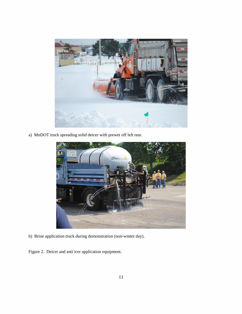
One technique of winter maintenance operations that has shown great promise is anti-icing, the pre-storm placement of deicer brine to clear pavement done to limit or prevent formation of icing on a roadway. Whether due to wind blown snow, ice fog, freezing rain, or simply wet snow becoming packed (Figure 1), anti-icing has been found to reduce formation and build up. However, winter maintenance operations have often found it difficult to mobilize the anti-icing application trucks, either because of labor shortages prior to a storm (resting crews before potential long shifts) or limited procurement of the anti-icing brine application equipment (Figure 2). Application of sodium chloride (rock salt) brine at typical rates between 10 and 30 gallons per lane mile (gal/LM) also provides a significant deicer material savings, as with a brine saturation of 23% concentration this rate calculates to 20 to 60 lb/LM, about 1/20th of the typical deicer application rate during a snow event.
However, anti-icing and deicing operations could be negatively affected by the roadway wetness as traffic removes salt through splash and spray as well as run off. Blomqvist, et al (2011) observed:
Road surface wetness, as shown from the wheel tracks, related positively to the rate of residual salt loss. The wetter the surface, the faster the salt left the wheel tracks. On a wet road surface, the salt in the wheel tracks was almost gone after only a couple of hundred vehicles had traveled across the surface, whereas on a moist road surface, it would take a couple of thousand vehicles to reach the same result.
The study described in this chapter aims to characterize and define the factors related to anti icer persistence during traffic and precipitation events, to minimize loss of anti icer material and maximize anti-icing performance. This study was done on an elevated section of an active highway as an outdoor test facility, employing actual anti-icing on actual traffic with operational winter maintenance efforts unadjusted for research. Factors evaluated included: deicer application rate, time, temperature, precipitation, and traffic situation.
2.1: Test Method
2.1.1: Method design
For this evaluation of anti-icing persistence, measurements of flow and deicer concentration over time were made of storm drainage runoff from defined highway pavement areas. Comparison of the deicer concentration in the runoff to the timing and amount of precipitation events can be assessed by factors including temperature and precipitation intensity. Comparison between

9
different pavement areas can allow evaluation of traffic factors including traffic rate, direction, truck proportion plus allow consideration of replicates for improvement of evaluation strength.
a) Wind blown snow b) Ice fog
c) Freezing rain d) Wet snow becoming packed
Figure 1. Winter conditions conducive to ice buildup on roadways.
2.1.2: Field Site
Pavement areas were defined by the contributing drainage area of individual scupper collection points on an elevated section of US 169 in Mankato, Minnesota (Figure 3), part of the Minnesota River crossing. This location was selected because: (1) the elevated highway is an active highway with known anti-icing and deicing procedures; (2) the drainage system is easy to access

10
from below, with no exposure to highway traffic nor any potential confined space entry as can occur with catch basins; and, (3) weather at this location was both sufficiently wintery and well defined through use of the National Oceanic and Atmospheric Agency (NOAA) weather system coverage.
Access agreements with MnDOT were negotiated and agreed upon on November 26, 2013, during a meeting with the District 7 Maintenance, Bridge and Hydraulics departments, the bridge managers. Safety procedure review was received at the bridge site on December 11, 2013, and project personnel were approved for site operations as proposed.
11
a) MnDOT truck spreading solid deicer with prewet off left rear.
b) Brine application truck during demonstration (non-winter day).
Figure 2. Deicer and anti icer application equipment.

12
a) Side view, view west.
b) Northbound lanes, view south.
Figure 3. North Star Bridge, US 169 over the Minnesota River at Mankato, Minnesota.

13
Bridge drainage follows the profile and crown slopes of the bridge deck, draining from south to north and from a crown line between the right and left lanes for both northbound and southbound directions. Drainage is collected from the pavement in scupper inlets, then flows downward through 8-inch ductile iron down chutes to discharge through an open bend to just above a concrete gutter on the ground surface that leads to a catch basin and a subsurface drainage system (Figure 4). Scuppers are located in sets of four located along a single bridge deck joint and coming down a single bridge pier line.
a) Scupper. b) Down chute piping, outside lane.
c) Down chute piping, inside lanes. d) Outlet to concrete drainage gutter.
Figure 4. North Star Bridge drainage.
Two sets of four scupper/down chute drainage features were selected for study, shown on Figure 5 and detailed in Table 1. The two sets are replicates, draining adjacent areas with the same traffic and thermal conditions. Each set of four scuppers represents four distinct areas of the bridge: northbound right lane, ramp and shoulder; northbound left lane with shoulder;

14
southbound left lane with shoulder; and southbound right lane, ramp and shoulder. The are denoted in that order as Locations A to D and E to H for the north and south sets, respectively. As viewed from the ground level, the north set is along the Minnesota River flood protection levee and the south set is near to Sibley Avenue.

15
Figure 5. North Star Bridge plan showing drainage inlet locations.

16
Table 1. Storm drainage locations used in measurements
Notation Direction, Station and Offset Lanes Drained Approximate Drainage Area
A
(Alfa)
TH 169 NB
Sta 107+40
32 ft right
Right through lane
Ramp lane
Shoulder
8,800 sf
B
(Bravo)
TH 169 NB
Sta 107+40
20 ft left
Left through lane
Shoulder
5,500 sf
C
(Charlie)
TH 169 SB
Sta 107+40
20 ft right
Left through lane
Shoulder
5,500 sf
D
(Delta)
TH 169 SB
Sta 107+40
32 ft left
Right through lane
Ramp lane
Shoulder
8,800 sf
E
(Echo)
TH 169 NB
Sta 104+65
32 ft right
Right through lane
Ramp lane
Shoulder
9,440 sf
F
(Foxtrot)
TH 169 NB
Sta 104+65
20 ft left
Left through lane
Shoulder
5,990 sf
G
(Golf)
TH 169 SB
Sta 104+65
20 ft right
Left through lane
Shoulder
5,990 sf
H TH 169 SB Right through lane 9,440 sf

17
(Hotel) Sta 104+65
32 ft left
Ramp lane
Shoulder
Notes: Station lines match to lines shown on plan of Figure 5. Locations A-D are at the north end of the elevated highway near the flood levee. Locations E-H are at the middle of the elevated highway near the north side of Sibley Parkway located below the highway. Names in parentheses beneath the notations were used during field operations to verbally distinguish locations; names may appear in field notes and calculations.
The traffic on the bridge was characterized for the project by Scott Thompson of MnDOT District 7:
The last time traffic counts were done on the bridge was 2011. At that time, the bridge had 32,500 AADT (Average Annual Daily Traffic). Of the 32,500 vehicles, 2,450 would be heavy commercial vehicles.
Traffic volumes in our area have been relatively flat. In order to inflate to 2014 values, I would use a straight 1% annual increase in volumes. Regarding directionality of the volumes, I would assume a 50/50 split. It should also be assumed that 10% of the daily traffic volume occurs during the peak AM rush hour and another 10% occurs during the peak PM rush hour.
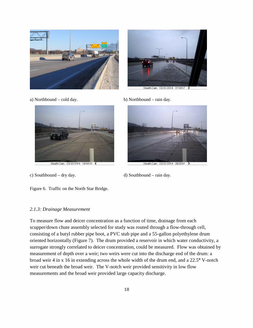
It may be noted that the heavy commercial (truck) proportion is about 7.5% of the total traffic. Figure 6 provides several views of traffic on the bridge.
18
a) Northbound – cold day. b) Northbound – rain day.
c) Southbound – dry day. d) Southbound – rain day.
Figure 6. Traffic on the North Star Bridge.
2.1.3: Drainage Measurement
To measure flow and deicer concentration as a function of time, drainage from each scupper/down chute assembly selected for study was routed through a flow-through cell, consisting of a butyl rubber pipe boot, a PVC stub pipe and a 55-gallon polyethylene drum oriented horizontally (Figure 7). The drum provided a reservoir in which water conductivity, a surrogate strongly correlated to deicer concentration, could be measured. Flow was obtained by measurement of depth over a weir; two weirs were cut into the discharge end of the drum: a broad weir 4 in x 16 in extending across the whole width of the drum end, and a 22.5° V-notch weir cut beneath the broad weir. The V-notch weir provided sensitivity in low flow measurements and the broad weir provided large capacity discharge.

19
Water level, conductivity and temperature were all measured using LTC Levelogger Junior in-water measurement probes (Solinst Canada, Ltd, Georgetown, ON), selected for both measurement ability and resistance to salt water. The probes were lowered into the drum and rested horizontally on the drum bottom until being removed for reading/downloading. PVC coated wire rope 1/8th in diameter was used to attach the Leveloggers to a U-bolt installed in the top crown of the horizontal drum. The drums were chained and locked in place, with the chain attaching to the ductile iron down chute above the lowest anchor point. The chain was also wrapped circumferentially around the drum and through an adjacent 8 in x 8 in x 16 in concrete masonry unit used to help level the drum and prevent the drum from rolling towards the center low point of the concrete gutter.
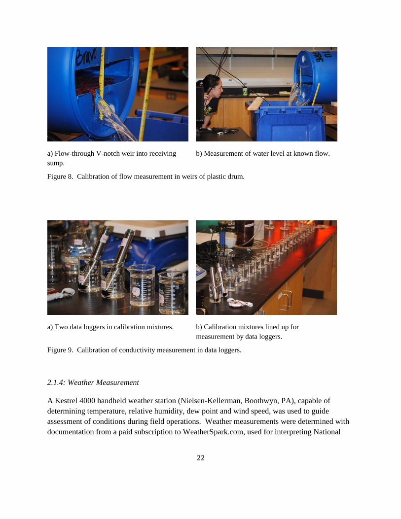
The weirs of each drum were calibrated for flow by pumping a known flow-through the drum then measuring the depth over the weir (Figure 8). A weir coefficient was obtained particular to each drum using a best fit method (Appendix A). Calibration was done for flows ranging from 0.2 gpm to 4 gpm. Additional evaluation was done for flows up to 50 gpm.
Conductivity calibration of each Levelogger was done using solutions made with sodium chloride (rock salt) at nine concentrations from 0 to 150 g/L (Figure 9 and Appendix B). Leveloggers were rinsed with deionized (DI) water, placed in the solution and read at four time intervals. The order of the solutions was randomized, and 36 total solution mixtures were evaluated. Results were evaluated and found to bifurcate with a lower range of 0 – 60 g/L and a higher range of 60 – 150 g/L best representing the measured conductivities. However, during the course of the 2013-14 winter season, no field measurements reached to the high range for the conductivity measurement.
Depth measurement was done by the Leveloggers using total pressure measured at pressure membrane location. Total pressure consists of atmospheric (barometric) pressure plus water pressure. To calculate water pressure, barometric pressure must be subtracted. Two barometric pressure loggers (Solinst Edge 3001 Barologger) were used in the project: a main Barologger locked to the flow-through cell at Location C and backup Barologger kept in the vehicle typically used to support the project (this vehicle was typically parked within ½ to 1½ miles of the North Star Bridge). Pressure and depth calibrations were done at the manufacture and provided with the instruments.
Clogging in the flow-through cells was frequently observed, typically consisting of cigarette butts, agricultural materials such as corn or soybeans, miscellaneous vegetative matter (Figure 10) or ice (Figure 11).

20
Because of the potential for ice to damage the pressure transducer within the Leveloggers, when temperatures were expected to be consistently below 20° F. flow-through cells were taken out of the drainage pathway and locked in place adjacent to the drainage gutter and down chute.

21
Figure 7. Flow-through cells
a) End view showing plastic drum with V-notch weir, broad weir, manual measurement tape, leveling chain/concrete masonry unit, and security chain.
b) Side view showing down chute piping, boot, PVC stub, plastic drum, leveling chain/concrete masonry unit, and security chain.
22
a) Flow-through V-notch weir into receiving sump.
b) Measurement of water level at known flow.
a) Two data loggers in calibration mixtures. b) Calibration mixtures lined up for measurement by data loggers.
Figure 8. Calibration of flow measurement in weirs of plastic drum.
Figure 9. Calibration of conductivity measurement in data loggers.
2.1.4: Weather Measurement
A Kestrel 4000 handheld weather station (Nielsen-Kellerman, Boothwyn, PA), capable of determining temperature, relative humidity, dew point and wind speed, was used to guide assessment of conditions during field operations. Weather measurements were determined with documentation from a paid subscription to WeatherSpark.com, used for interpreting National

23
Weather Service data obtained from Mankato Regional Airport, located 6 miles northeast of the field site.
Figure 10. Debris clog at Location A, March 27, 2014.
2.1.5: Cameras and Photography
Field conditions were documented through photography using two different camera systems. Handheld, high resolution photographs were taken using a Nikon D3000 camera with a 55-200 mm telephoto lens, occasionally alternating with a 20-55 mm wide angle lens. Time-lapse photographs were taken using Stealth Calm Core 3 time-lapse (game scouting) cameras (Figure 9) (Stealth Cam, LLC, Grand Prairie, TX). Time-lapse cameras were pole mounted at approximately a 2-ft height for flow-through cell observations. Time lapse cameras were installed on March 26, 2014 and remained in place through April 12th, taking photographs at 5 minute increments from 7 am to 7 pm.
2.1.6: Plow and Deicer Spreading Operations
Plowing and deicer spreading (distribution) were done by maintenance personnel from MnDOT District 7 Headquarters location in Mankato. Typical equipment was a Sterling tandem axle,

24
automatic transmission dump truck with front, right wing and underbody plows (Figure 2a). Side mounted (saddle) tanks were used to carry brine materials used for prewetting granular deicer. Typical deicer material applied was rock salt pretreated with calcium chloride at a rate of 6 gal/ton then prewet with salt brine (sodium chloride, 23.3%). Application typically is off the left rear corner of an application truck, so placed to use traffic for pavement distribution. Based on discussion with maintenance personnel, the North Star Bridge was treated with deicer at about 400 lb/LM three days a week as an anti-icing treatment, plus application of 200 – 800 lb/LM during storm event plowing. Application rates were automatically adjusted for vehicle speed.

25
a) March 27, 2014, Location F, ice level above broad weir.
b) April 3, 2014, Location F, debris and ice damming flow-through V-notch weir.
Figure 11. Ice blocking.

26
2.2: Results
Events and manual flow measurements pertaining to North Star Bridge locations are provided in Table 2. Data was collected in 5-minute increments by the Leveloggers then supplemented with manual measurements to provide a check. Results from each measurement location at the North
Star Bridge are presented in Appendix D by location (denoted as separate sub appendices). Results are presented in two graphs on a page: conductivity and temperature graphed to separate scales on the top graph, water level and temperature similarly graphed to separate scales on the bottom graph (temperature is used as a marker for comparison between the two graphs). Within each sub appendix, results are first presented for the whole testing period of February 16th to April 6th, 2014, showing a gap for weather too cold for Levelogger deployment from February 21st to March 7th. Additional presentation of results follows using time periods of deployment weeks, allowing for greater detail per graph, using a calendar format to the graphs representing a typical calendar week of Sunday to Saturday.
Calculation of chloride concentration and flow at each location was done, with results presented graphically in Appendix E by location (same organizational structure and graphing system as Appendix D). Chloride concentration was calculated using the Levelogger specific conductivity and the calibration relationship developed as shown in Appendix B. Flow was calculated using values for the height of water over a flow-through cell weir, obtained from the Levelogger depth less a zero-flow depth representing the submersion level of the logger. Zero-flow depths were determined manually from the graphs of water depth in Appendix D for periods of no flow. Zero-flow depths were reassessed for time periods after Levelogger download or adjustment (e.g., cleaning), or for periods following obvious icing.
Calculation of mass flow, defined as the amount of mass passing a drainage location in a period of time, was calculated from the results of Appendix E by the formula:
Mass Flow = Mass/Time = Concentration x Flow (Equation 1)
Mass flow was determined in units of lb/LM/minute to show a running level related to the application of deicer and anti icer.
Cumulative mass flow, defined as the sum of all the mass flow that had passed through a drainage location, was determined on a weekly basis beginning at 12:00 am on a given Sunday (start point arbitrarily picked to match the graphing interval). Cumulative mass flow was determined in units of lb/LM/week to show a running level related to the application of deicer and anti icer.

27
Both mass flow and cumulative mass flow are presented graphically in Appendix F by location (same organizational structure and graphing system as Appendices D and E). Ideally, these values would be accompanied by automatic vehicle locator (AVL) system results that include the deicer application rates. However, AVL results were apparently not recorded for the North Star Bridge treatments during the study period.

28
Table 2. Events and flow measurements pertaining to North Star Bridge locations.
Date
Comments
Measured Flows by Location (L/min)
A B C D E F G H
2/16 Deployed equipment. X X X X X X X X
2/20 Precipitation 1 – 3 pm.
Measured flows then removed equipment ~4 pm.
5.7 0.4 0.4 12 5.0 X 0.4 17
3/7 Reinstalled equipment (A-D, F & G).
Snow observed on bridge to be in windrows along parapet and median walls.
0.4 0.1 0.2 ~0 X 0.2 0.2 X
3/11 Precipitation 8 – 10 am. X X X X X X X X
3/12 Loggers frozen in at Locations A-D, F & G. Reinstalled loggers at Locations E & H.
0 0 0 0 0 0 0 0
3/13 All loggers frozen in. ~0 ~0 ~0 ~0 ~0 ~0 ~0 ~0
3/14 All loggers melted out. Downloaded, cleaned and reset loggers.
0 0 0 0 0 0 0 0
3/20 Downloaded, cleaned and reset loggers. Location F clogged by ice block. Other
locations ice free. 0 0 0 1.0e 0 0 0 1.0e
3/26 All loggers frozen in; ice ~3 inches thick. 0 0 0 0 0 0 0 0
3/27
Precipitation 1 – 7 pm.
Cleaned weirs of clogs. Estimated flows at 3 pm. Locations E – H drowned/flows
backed up through weirs.
6e 3 e 2 e 3 e 10 e 6 e 3 e 12 e
3/30 Downloaded, cleaned and reset loggers. 0 0 0 0 0 0 0 0
3/31 Precipitation 9 – 10 am. X X X X X X X X
4/3
Precipitation 6 – 7 pm.
Flows measured at 5 pm prior to rain. Flows observed to suddenly increase up to
X X X X 2 0.9 0.5 1.8
29
25 L/min estimated.
4/7 Removed equipment 4 pm. X X X X X X X X
Notes: X: not measured. e: flow estimated. ~0: flow approximately zero; a dribble.
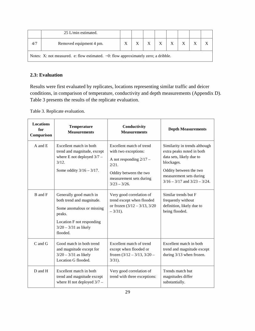
2.3: Evaluation
Results were first evaluated by replicates, locations representing similar traffic and deicer conditions, in comparison of temperature, conductivity and depth measurements (Appendix D). Table 3 presents the results of the replicate evaluation.
Table 3. Replicate evaluation.
Locations for
Comparison
Temperature Measurements
Conductivity Measurements
Depth Measurements
A and E Excellent match in both trend and magnitude, except where E not deployed 3/7 – 3/12.
Some oddity 3/16 – 3/17.
Excellent match of trend with two exceptions:
A not responding 2/17 – 2/21.
Oddity between the two measurement sets during 3/23 – 3/26.
Similarity in trends although extra peaks noted in both data sets, likely due to blockages.
Oddity between the two measurement sets during 3/16 – 3/17 and 3/23 – 3/24.
B and F Generally good match in both trend and magnitude.
Some anomalous or missing peaks.
Location F not responding 3/20 – 3/31 as likely flooded.
Very good correlation of trend except when flooded or frozen (3/12 – 3/13, 3/20 – 3/31).
Similar trends but F frequently without definition, likely due to being flooded.
C and G Good match in both trend and magnitude except for 3/20 – 3/31 as likely Location G flooded.
Excellent match of trend except when flooded or frozen (3/12 – 3/13, 3/20 – 3/31).
Excellent match in both trend and magnitude except during 3/13 when frozen.
D and H Excellent match in both trend and magnitude except where H not deployed 3/7 –
Very good correlation of trend with three exceptions:
Trends match but magnitudes differ substantially.

30
3/12. D exhibits extra peak 2/17.
Oddity between the two measurement sets during 3/23 – 3/26 when frozen.
H increased abruptly on 4/1 and stayed elevated; not seen with D.
H has extra peaks 2/17 – 2/18.
Very different magnitudes observed during periods when frozen.
Replicate comparison may be summarized by the following observations:
• All locations were impacted when frozen, as large oddities in depth measurements were caused by ice pressure, and muting of conductivity response during melt out was caused by inability of flow to mix around the logger;
• Locations F and G were often compromised by flooding of the weirs due to slow drainage away from the locations;
• Location H was impacted by freezing/potential blockage in down chute; • Temperature measurements generally were excellent matches of both trend and
magnitude; • Conductivity measurements generally were excellent matches of trend and good
correlates of magnitude; and, • Depth measurements generally were good matches of trend but exhibit jumps likely due
to blockage or ice.
Both conductivity and depth measurements were seen to appropriately respond to precipitation.
2.3.1: Comparison of Chloride Mass Flow Rates and Cumulative Weekly Amounts
Chloride mass flow rates were taken from the graphs in Appendix E for each week of the study period. Maximum rate magnitudes are provided in Table 4, and cumulative mass per week are provided in Table 5. Magnitudes of maximum rates seem consistent throughout the study period and across the drainage locations, though issues were observed due to anomalous flow calculations likely due to either ice pressure on the depth loggers or back-flooding of the flow calculation weirs. Location H also experienced impacts from blocked down chute (Figure 12) that existed during March. No extreme swings in maximum chloride mass flow rate were observed except when influenced by the previously mentioned issues. No behavioral patterns were observed due to factors represented by drainage measurement location such as traffic lane, traffic direction.
31
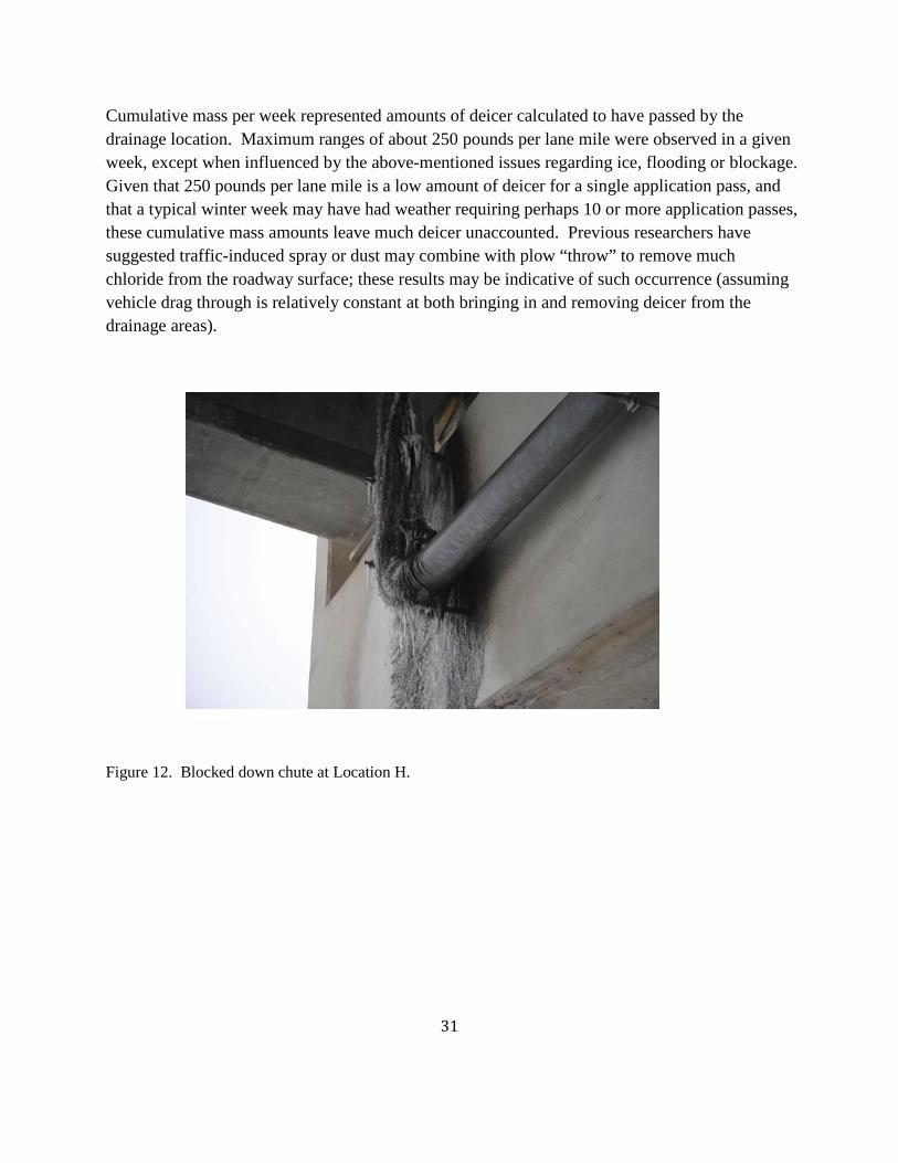
Cumulative mass per week represented amounts of deicer calculated to have passed by the drainage location. Maximum ranges of about 250 pounds per lane mile were observed in a given week, except when influenced by the above-mentioned issues regarding ice, flooding or blockage. Given that 250 pounds per lane mile is a low amount of deicer for a single application pass, and that a typical winter week may have had weather requiring perhaps 10 or more application passes, these cumulative mass amounts leave much deicer unaccounted. Previous researchers have suggested traffic-induced spray or dust may combine with plow “throw” to remove much chloride from the roadway surface; these results may be indicative of such occurrence (assuming vehicle drag through is relatively constant at both bringing in and removing deicer from the drainage areas).
Figure 12. Blocked down chute at Location H.
32
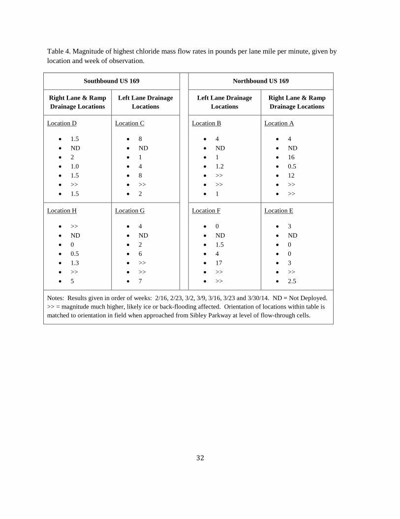
Table 4. Magnitude of highest chloride mass flow rates in pounds per lane mile per minute, given by location and week of observation.
Southbound US 169 Northbound US 169
Right Lane & Ramp Drainage Locations
Left Lane Drainage Locations
Left Lane Drainage Locations
Right Lane & Ramp Drainage Locations
Location D
• 1.5 • ND • 2 • 1.0 • 1.5 • >> • 1.5
Location C
• 8 • ND • 1 • 4 • 8 • >> • 2
Location B
• 4 • ND • 1 • 1.2 • >> • >> • 1
Location A
• 4 • ND • 16 • 0.5 • 12 • >> • >>
Location H
• >> • ND • 0 • 0.5 • 1.3 • >> • 5
Location G
• 4 • ND • 2 • 6 • >> • >> • 7
Location F
• 0 • ND • 1.5 • 4 • 17 • >> • >>
Location E
• 3 • ND • 0 • 0 • 3 • >> • 2.5
Notes: Results given in order of weeks: 2/16, 2/23, 3/2, 3/9, 3/16, 3/23 and 3/30/14. ND = Not Deployed. >> = magnitude much higher, likely ice or back-flooding affected. Orientation of locations within table is matched to orientation in field when approached from Sibley Parkway at level of flow-through cells.

33
Table 5. Magnitude of cumulative chloride mass flow rates in pounds per lane mile per week, given by location and week of observation.
Southbound US 169 Northbound US 169
Right Lane & Ramp Drainage Locations
Left Lane Drainage Locations
Left Lane Drainage Locations
Right Lane & Ramp Drainage Locations
Location D
• 160 • ND • 40 • 60 • 500 • >> • 40
Location C
• 200 • ND • 100 • 200 • 2000 • >> • 160
Location B
• 50 • ND • 15 • 20 • >> • >> • 20
Location A
• 200 • ND • 2500 • 2500 • 3000 • >> • >>
Location H
• >> • ND • 20 • 20 • 20 • >> • 300
Location G
• 100 • ND • 25 • 70 • >> • >> • 160
Location F
• 2 • ND • 7.5 • 1600 • >> • >> • >>
Location E
• 220 • ND • 0 • 1 • 350 • >> • 125
Notes: Results given in order of weeks: 2/16, 2/23, 3/2, 3/9, 3/16, 3/23 and 3/30/14. ND = Not Deployed. >> = magnitude much higher, likely ice or back-flooding affected. Orientation of locations within table is matched to orientation in field when approached from Sibley Parkway at level of flow-through cells.
2.3.2: Comparison of Traffic Effects by Storm Event
Chloride amounts measured at individual drainage locations were compared for five storm events (Table 6) for magnitude and timing differences attributable to traffic condition. These storm events encompass the precipitation events with potential for near-freezing temperatures that occurred during the period when the flow-through cells were deployed and unaffected by ice buildup during the study period (February to April). Comparing results, it may be observed that little difference in timing of deicer flow was noted between drainage locations. Magnitude differences were not found due to traffic differences, although perhaps application differences influenced some results as occasions were noted when little or no deicer appeared to have been applied to certain lanes. No persistence was observed between storm events, illustrated by the

34
March 31st storm passing effectively no deicer only four days after the previous storm that had deicer use. Interestingly, during the March 11th storm, potential effect of wind was observed in that deicer was measured for the eastern portion of each highway segment, perhaps due to a crossing wind.
Table 6. Comparison of cumulative chloride mass magnitude and timing by traffic conditions for specific storm events.
Storm Event Right Lane and Ramp Areas
Left Lane Areas Northbound US 169
Southbound US 169
2/20 noon – 6 pm, 30° F, 0.043 inch.
NB and SB are similar in timing. Magnitude of NB is about twice SB.
Low magnitude observed. NB and SB are similar.
Right lane magnitude much larger than left lane. Timings similar.
Right lane magnitude much larger than left lane. Timings similar.
3/11 6 am – noon, 36° F, 0.032 inch.
NB magnitude much larger than SB, perhaps 12x. Timings similar.
SB magnitude much larger than NB, perhaps 6x. Timings similar.
Right lane magnitude about 3x left lane magnitude.
Left lane magnitude about 3x right lane magnitude.
East side of each highway has ~6x magnitude greater than corresponding west side.
3/27 noon – 6 pm, 37° F, 0.166 inch.
SB ~ 20 lbs/LM greater than NB. Timings similar.
SB ~ 20 lbs/LM greater than NB. Timings similar.
Only right lane exhibits deicer.
Right and left lane magnitudes similar.
3/31 6 am – noon, 30° F, 0.043 inch.
No chloride measured above 1 pound per lane mile except at Location G (~10 pounds per lane mile).
2/20 3 pm – 9 pm, 32° F, 0.022 inch.
NB & SB similar; magnitudes low. Timings similar.
NB & SB similar; magnitudes low. Timings similar.
Right lane magnitude 3x left lane. Timings similar.
Right and left lane magnitudes and timings similar.
Notes: Precipitation amounts from NOAA Doppler radar summation. NB = Northbound. SB = Southbound.
35
2.4: Conclusions and Recommendations
A deicer and anti icer test facility was set up and procedures established. Eight drainage locations of US 169 were routed through flow cells for measurements of chloride content and flow. Comparisons suggested good experimental behavior in the method, excepting anomalous readings caused by instruments frozen in ice and effects caused by debris blockage. Efforts to protect and clean gear during deployment increased reliability. Of the measurements, it was observed that:
• Temperature makes a good variable to check on instrument operating conditions; • Conductivity and therefore chloride concentration were only affected by a lack of mixing
due to ice or sedimentation in the flow-through cells; and, • Depth and therefore flow measurement were sensitive to ice buildup and debris blockage.
Individual drainage measurement locations experienced some site-specific impact due to blockage in down chute (Location H) or outlet back-flooding (Location F); it is recommended that each location be closely monitored in future efforts. Time lapse photography could be employed to aid in location and equipment monitoring.
Chloride mass amounts passing through the drainage locations were calculated at levels substantially below the likely roadway application levels. This observation was consistent through the study area, regardless of traffic condition or direction. This finding agrees with observations by previous researchers that the majority of deicer loss occurs through traffic-induced spray or dust combined with plow “throw”. It is recommended that future efforts incorporate atmospheric sampling and off-roadway drainage measurement to assess chloride migration through such effects. Some evidence was observed of possible wind effects in the pathway of chloride on the roadways of the study site.
Results of two closely spaced storms suggested little to no persistence in chloride after a storm event. This result was intriguing, as it indicates that anti-icing may be detrimentally affected by any antecedent moisture prior to the anticipated icing event. Additional evaluation of this effect will occur during the upcoming Task 4 Pavement Study of this contract.
Because of the severe conditions during the winter of 2013-14 (coldest winter in 30+ years), only late winter conditions were available for evaluation. Therefore, declining temperature conditions associated with early winter were not able to be tested. Additionally, deicer application rates and frequency may have been affected by reduced availability of rock salt during the late winter after very high seasonal usage within the Upper Midwest region. Lastly, for the period of this study, AVL records of deicer application at the study facility were apparently not recorded and

36
therefore could not be used for comparison. It is hoped that future evaluations will be done for early winter conditions and with full AVL results for comparison.
Vandalism was not an issue during the study period, in spite of the area showing signs of frequent pedestrian traffic and warnings from local officials. Perhaps the severe winter temperatures helped protect the equipment. When equipment was removed in mid April, footprints and bike tire tracks were noted around some study locations.
Chapter 3: Deicer Effectiveness Study
This study aims to characterize and define these factors by developing and using an outdoor pavement facility with nine 1000-ft long lanes for treatment areas, separated to prevent incidental cross-treatment, located in Shakopee, Minnesota, at two proximal locations. The length of treatment areas was set to provide sufficient room for normal highway operating speeds of spreader vehicles (plow trucks). Time-lapse cameras were placed sufficiently close to treatment areas to observe and document deicing in high definition. Deicer were applied by MnDOT Metro District spreader trucks on non-storm days. Factors evaluated included: temperature at application, deicer rate of application use of prewetting agent, traffic, weather, and wind condition.
3.1: Test Method
3.1.1: Method Design
For this evaluation of deicing effectiveness and contributing factors, pavement lanes were set up and defined where deicers could be applied without actual traffic such that experimental approaches could be tried out and compared without potential for compromising public safety.
Lane lengths of 900 to 1000 ft long were defined, plus additional space for turning, so that spreader trucks could reach and maintain highway speeds of approximately 30 mph. Time-lapse and hand held camera photographs were used to augment observation notes and to document the activity and progress of deicers.
Deicer approaches were compared both within the conditions of a given day and under different weather conditions between days. Actual snow conditions were used, supported by ice sheets created for additional evaluation. MnDOT spreader trucks were used on non-storm days to closely model actual efforts without significantly diverting equipment necessary for actual road maintenance during storms.

37
3.1.2: Field Sites
Shakopee was targeted for project field sites to provide locations accessible both to researchers from Minnesota State, Mankato and maintenance personnel of MnDOT Metro District, with potential for additional access by maintenance personnel of other nearby MnDOT Districts.
Pavement lanes were set up in Shakopee at two locations with large parking lots not typically used during winter months:
• Canterbury Park, 1100 Canterbury Road; in the overflow parking lot on the north side of the facility, approximately 0.25 mile south of 4th Avenue East and 0.5 mile west of Canterbury Road South (Figure 13a).
• Valleyfair, One Valleyfair Drive; in the back (north) parking lot on the north east corner of the facility, located north of TH 101 about 2.5 miles west of US 169 (Figure 13b).

38
•
a) Canterbury Park
b) Valleyfair
Figure 13. Pavement areas with snow cover prior to plowing.
39
Access agreements were negotiated and agreed upon during early December, 2013. Prior to a lasting snowfall, researchers with support from MnDOT Metro District maintenance staff performed pavement surveys to locate and document surface discontinuities (Figure 14) that could either interfere with or be damaged by plowing. Test lanes were configured to avoid such discontinuities. Lane marking was done with pin flags of various colors; colors were assigned to designate the sides of individual lanes. Pin flags were anchored through 6 in x 3 in x 2 in “sewer” (hollow core) bricks to 8 in x 8 in x ¾ in wooden plates and stabilized by 1 ft lengths of ¾ in diameter Schedule 40 PVC pipe. Anchoring was done to prevent penetration of the pavement by the flags yet maintain the flags in spite of winter winds. Initial lane cuts were made December 18th (Figure 15); afterwards flags were reset on measured locations to represent 100-ft stationing along both sides of each lane (Figure 16). Completed lanes are shown in Figure 17, from conditions representative of early January, 2014.
Figure 18 shows the benefit of having two separate locations involved in the study. Lanes at Canterbury Park were located on top of a low ridge, and therefore were exposed and often had transverse snow drifts. Conversely, lanes at Valleyfair were located in an area of river bottomland, protected by mature trees on the parking lot perimeter, and therefore were protected and often had uniform snow.
Formation of ice sheets by which to test deicers was explored on January 8th and 10th, 2014. Approximately 100 gal of tap water was obtained from a laboratory at Minnesota State, placed in two horizontally mounted 55-gal drums located in a 7-passenger van, and transported to the Canterbury Park field site. With temperatures at -5°F on January 8th, ice formation techniques tested included:
• Pouring water directly from 5-gal buckets (Figure 19a); • Drizzling water via hoses from the 55-gal drums (Figure 19b); • Spraying water from woodland fire suppression bladder bag and hand pump (Figure 19c);
and, • Directly pouring from the 55-gal drums (Figure 19d).
Figures 7e and 7f show the comparison between unconsolidated snow, left after plowing at -5°F, and consolidated snow and ice formed by direct pouring of water from 5-gal buckets.
Direct pouring water from the 5-gal buckets was found to be the most efficacious method for forming ice sheets, although water consumption was relatively high. Hose drizzling was too slow a method to cover areas larger than perhaps 10 ft long, at least without additional pressurization. Hand pump spraying of water provided a uniform surface, but thin. Hand pump was also subject to frequent ice clogging at the pump nozzle (unblocked by momentary

40
immersion in water). Direct pouring water from the 55-gal drums was limited to amounts that could be lifted.
At -5°F, ice was created with limited drainage off-lane (wasted water and effort). However, at 28°F on January 10th, applied water was found to melt previously formed ice (water applied via direct pouring from 5-gal buckets). Water obtained from Minnesota State was approximately 50°F and did not appreciably cool during the 1 hr transport time. When ice formation is needed in the future, it is recommended that water be cooled prior to application, though the thermal stability of water is such that techniques will need to be developed for different levels of ambient winter temperatures.
a) Drainage structure at Canterbury Park b) Transverse drainage gutter at Valleyfair
Figure 14. Pavement discontinuities, noted prior to snowfall.
a) Canterbury Park b) Valleyfair
Figure 15. First snowplow cuts.

41
Figure 16. Placement of lane marking flags and stationing of lane distance.

42
a) Canterbury Park
b) Valleyfair
Figure 17. Completed lanes.

43
a) Canterbury Park February 13, 2014 showing wind effects and creation of drift structure.
b) Valleyfair January 8, 2014 showing uniformity of conditions created by river bottomland and tree protection.
Figure 18. Comparison of conditions possible between field sites.
3.1.3: Weather Measurement
A Kestrel 4000 handheld weather station (Nielsen-Kellerman, Boothwyn, PA), capable of determining temperature, relative humidity, dew point and wind speed, was used to determine conditions during field operations (Figure 20a). A dial thermometer (Figure 20b) was used for illustration and photographic documentation, but was not considered sufficiently accurate to represent field conditions. Weather measurements were augmented with documentation from a paid subscription to WeatherSpark.com, used for interpreting National Weather Service data obtained from Flying Cloud Airport, Eden Prairie, Minnesota, approximately 2 miles north of either field site.
3.1.4: Cameras and Photography
Field conditions were documented through photography using two different camera systems. Handheld, high resolution photographs were taken using a Nikon D3000 camera with a 55-200 mm telephoto lens, occasionally alternating with a 20-55 mm wide angle lens. Time-lapse photographs were taken using Stealth Calm Core 3 time-lapse (game scouting) cameras (Figure 21) (Stealth Cam, LLC, Grand Prairie, TX). Time-lapse cameras were pole mounted at approximately a 6-ft height, with poles attached to wooden bases. Wooden bases were set aside once windrows built up along test lanes, as poles were directly inserted into windrows for support. Typically, time-lapse cameras were installed at lane station 1+00 for each lane, meaning 100 ft from the start of the lane, oriented in the direction of the plow and deicer truck movement. Time increments of 1 minute were typically used. Date and time stamps were made on time-lapse photographs, though all photographs had file origination information that could provide time of capture for verification, if needed.

44
a) Pour from buckets. b) Hose drizzle.
c) Woodland fire suppression bladder bag spray. d) Direct pour from transport drum.
e) Post plow, pre-icing treatment surface. Note significant amount of unconsolidated snow.
f) Post-icing treatment surface with ice formation.
Figure 19. Exploration of techniques to create ice sheet patches on pavement lanes.

45
a) Handheld weather station. b) Dial thermometer.
Figure 20. Weather monitoring tools.
3.1.5: Plow and Deicer Spreading Operations
Plowing and deicer spreading (distribution) were done by maintenance personnel from MnDOT Metro District using equipment from the Chaska Truck Station. Typical equipment was a 2006 Sterling tandem axle, automatic transmission dump truck with front, right wing and underbody plows (Figure 22a). Side mounted (saddle) tanks were used to carry brine materials used for prewetting granular deicer (Figure 22b). A transverse auger was mounted in the rear of the dump body to feed deicer either to the left or right chute. Granular deicer was maintained in contact with the auger by frequent plow body raising such that the granular deicer would shift to the back of the plow body where the auger was located. Deicer would fall through the chute to a distributor (spinner) plate (Figure 22c). Prewet was poured via gravity onto the granular deicer when on the distributor plate (Figure 22d). The distributor plate rotated when the truck was in forward motion, spreading deicer rather than having a straight drop (Figure 23).
Alternative truck configurations were also used during plowing and deicing operations, typically consisting of single axle trucks or trucks with manual transmission. Note that Metro District deicer application equipment on board trucks was calibrated at the start of the 2013-14 season, according to the maintenance staff.

46
a) Time-lapse camera, pole mounted. b) Pole mounted cameras with detachable bases being deployed.
c) Pole mounted cameras directly inserted into plow windrows.
d) Camera in foreground with view of lane prior to plowing.
e) Truck passing pole mounted camera on left. f) Camera view after truck has just past.
Figure 21. Time-lapse cameras and a resulting photograph.

47
a) MnDOT tandem axle dump truck with front and right wing plows engaged.
b) MnDOT truck with saddle tanks for prewet fluid.
c) Salt distributor behind left rear wheel (not in motion/not being fed deicer at time of photo).
d) Prewet flow onto salt distributor (not in motion/not being fed deicer at time of photo).
Figure 22. Plow and deicer equipment on a MnDOT truck used for this study.

48
Figure 23. MnDOT truck spreading deicer off left rear while moving forward with a right-angled front plow.
3.2: Results
Field activities related to deicing evaluation are listed in Table 7, by date and weather conditions. Individual lane treatments are listed in Tables 8 to 11 for each date of testing and evaluation.
Documentation of weather conditions was obtained from the National Weather Service station at the Flying Cloud Airport, Eden Prairie, Minnesota, approximately 2 miles north of either site. Data was interpreted using the WeatherSpark.com web service, in a paid subscription. Graphical representations for each day of field activities, and including a few days prior weather, are provided in Appendix F as pages 1 to 7. Documentation of daily increments for the whole testing season from November to mid March are also included in Appendix F as pages 8 and 9.
Time-lapse photography was used for four field days when plowing and deicing activities were done on over the full distance of a pavement lane. Specific dates include:
• January 29, 2014 • February 6, 2014 • February 14, 2014, and • February 19, 2014.

49
Time-lapse photographs of each lane during plowing and deicing activities are provided in summary form in Appendix G. Time-lapse photographs are provided for times prior to plowing, immediately after plowing, then 10, 20, 30 and 60 minutes after plowing. Where noted, “camera malfunction” typically represents a camera that did not withstand the snow thrown by the passing plow; photographs of the lane were therefore not obtained until the camera was picked up and repositioned.
Table 7. Deicing activities by date and weather conditions
Date Weather Deicing Activities
12/18/2013 5°F, clear and sunny
wind 0-3 mph
Plowing only; initial cutting of lanes and installation of stationing flags
1/8/2014 -5°F, clear and sunny
wind 5 mph
Plowing only; Canterbury Park only; recutting lanes
1/10/2014 28°F, overcast
wind 10-15 mph
Spot treatments on prepared ice sheets
1/29/2014 25°F, clear and sunny
wind 5-15 mph
200 to 800#/LM rock salt; prewet/no prewet; car traffic/no traffic
2/6/2014 4°F, clear and sunny
wind 8-12 mph
200 to 800#/LM rock salt; prewet/no prewet; car traffic/no traffic
Repeat of 1/29/2014 with colder temperatures
2/14/2014 13°F, clear and sunny
wind 8-12 mph
800#/LM rock salt; prewet/no prewet; car traffic/truck traffic/no traffic
2/19/2014 40°F, clear and sunny
wind 0-3 mph
800#/LM rock salt; prewet/no prewet; car traffic/truck traffic/no traffic
Repeat of 2/14/2014 with warmer temperatures
Note: There was insufficient snow cover before 12/3/2013 by which to plow and deice; there was insufficient cold as of 3/6/2014 to maintain snow cover until MnDOT plow and deicing trucks were available.

50
Prior to December 18, 2013, snow remaining the day after a storm event was insufficient for testing and evaluation. On March 6, 2014, an additional day of plowing and deicing was planned; however, melting of snow created slick conditions underlying the snow. A MnDOT truck mounted plow was unable to clear access to the pavement lanes at Canterbury Park, resulting in test cancelation. By March 13, 2014, insufficient snow remained on the pavement lanes for additional testing.
Table 8. Deicing activities by lane for 1/29/2014, at 25°F, clear and sunny, with wind 5-15 mph.
Lane Deicer, Rate & Prewet Condition
Traffic Condition
CD1 Rock Salt, 200#/LM LCS prewet, 15 gal/ton
No traffic
CD2 Rock Salt, 400#/LM LCS prewet, 15 gal/ton
No traffic
CD3 Rock Salt, 800#/LM LCS prewet, 15 gal/ton
No traffic
CD4 Rock Salt, 400#/LM No prewet
No traffic
CD5 Rock Salt, 400#/LM LCS prewet, 15 gal/ton
Car, 5 passes beginning ~60 min after deicer application
CD6 Rock Salt, 400#/LM No prewet
Car, 5 passes beginning ~60 min after deicer application
VF1 Rock Salt, 400#/LM LCS prewet, 15 gal/ton
No traffic
VF2 Rock Salt, 800#/LM LCS prewet, 15 gal/ton
No traffic
VF3 Rock Salt, 400#/LM No prewet
No traffic
Note: CD denotes a lane at Canterbury Park (Canterbury Downs); VF denotes a lane at Valleyfair. Lanes are numbered increasing from north to south at each parking lots.

51
Table 9. Deicing activities by lane for 2/6/2014, at 4°F, clear and sunny, with wind 8-12 mph.
Lane Deicer, Rate & Prewet Condition
Traffic Condition
CD1 Rock Salt, 200#/LM
LCS prewet, 15 gal/ton No traffic
CD2 Rock Salt, 400#/LM
LCS prewet, 15 gal/ton No traffic
CD3 Rock Salt, 800#/LM
LCS prewet, 15 gal/ton No traffic
CD4 Rock Salt, 400#/LM
No prewet No traffic
CD5 Rock Salt, 400#/LM
LCS prewet, 15 gal/ton
Car, 5 passes beginning ~60 min after deicer application
CD6 Rock Salt, 400#/LM
No prewet
Car, 5 passes beginning ~60 min after deicer application
VF1 Rock Salt, 400#/LM
LCS prewet, 15 gal/ton No traffic
VF2 Rock Salt, 800#/LM
LCS prewet, 15 gal/ton No traffic
VF3 Rock Salt, 400#/LM
No prewet No traffic
Note: CD denotes a lane at Canterbury Park (Canterbury Downs); VF denotes a lane at Valleyfair. Lanes are numbered increasing from north to south at each parking lots.
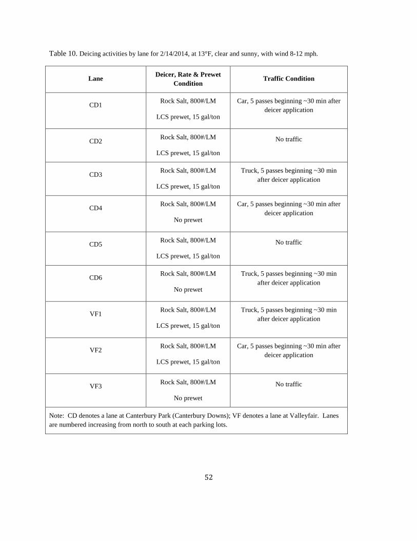
52
Table 10. Deicing activities by lane for 2/14/2014, at 13°F, clear and sunny, with wind 8-12 mph.
Lane Deicer, Rate & Prewet Condition
Traffic Condition
CD1 Rock Salt, 800#/LM
LCS prewet, 15 gal/ton
Car, 5 passes beginning ~30 min after deicer application
CD2 Rock Salt, 800#/LM
LCS prewet, 15 gal/ton
No traffic
CD3 Rock Salt, 800#/LM
LCS prewet, 15 gal/ton
Truck, 5 passes beginning ~30 min after deicer application
CD4 Rock Salt, 800#/LM
No prewet
Car, 5 passes beginning ~30 min after deicer application
CD5 Rock Salt, 800#/LM
LCS prewet, 15 gal/ton
No traffic
CD6 Rock Salt, 800#/LM
No prewet
Truck, 5 passes beginning ~30 min after deicer application
VF1 Rock Salt, 800#/LM
LCS prewet, 15 gal/ton
Truck, 5 passes beginning ~30 min after deicer application
VF2 Rock Salt, 800#/LM
LCS prewet, 15 gal/ton
Car, 5 passes beginning ~30 min after deicer application
VF3 Rock Salt, 800#/LM
No prewet
No traffic
Note: CD denotes a lane at Canterbury Park (Canterbury Downs); VF denotes a lane at Valleyfair. Lanes are numbered increasing from north to south at each parking lots.

53
Table 11. Deicing activities by lane for 2/19/2014, at 40°F, clear and sunny, with wind 0-3 mph.
Lane Deicer, Rate & Prewet Condition
Traffic Condition
CD1 Rock Salt, 800#/LM
LCS prewet, 15 gal/ton
Car, 5 passes beginning ~30 min after deicer application
CD2 Rock Salt, 800#/LM
LCS prewet, 15 gal/ton
No traffic
CD3 Rock Salt, 800#/LM
LCS prewet, 15 gal/ton
Truck, 5 passes beginning ~30 after deicer application
min
CD4 Rock Salt, 800#/LM
No prewet
Car, 5 passes beginning ~30 min after deicer application
CD5 Rock Salt, 800#/LM
LCS prewet, 15 gal/ton
No traffic
CD6 Rock Salt, 800#/LM
No prewet
Truck, 5 passes beginning ~30 after deicer application
min
VF1 Rock Salt, 800#/LM
LCS prewet, 15 gal/ton
Truck, 5 passes beginning ~30 after deicer application
min
VF2 Rock Salt, 800#/LM
LCS prewet, 15 gal/ton
Car, 5 passes beginning ~30 min after deicer application
VF3 Rock Salt, 800#/LM
No prewet
No traffic
Note: CD denotes a lane at Canterbury Park (Canterbury Downs); VF denotes a lane at Valleyfair.are numbered increasing from north to south at each parking lots.
Lanes

54
3.3: Evaluation
The objective of deicing for this project was improvement in open, un-iced pavement, primarily observed as enlargement of the un-iced patches, interpreted to represent improved driving conditions. Evaluation of deicing results was made for selected factors using time-lapse photography of treated lanes, primarily represented by the photographs presented in Appendix G. Additional evaluation was done using hand-held (Nikon) photographs, presented in Appendices H – J for specific factor evaluation.
3.3.1: Effect of Time and Temperature
Time and temperature are critical factors for deicing, in that a quicker melt will improve roadways sooner and that deicer performance is significantly temperature dependent (Table 12). Deicer performance is generally a function of ice melt capacity, defined as the amount of ice melted (brine created) per the amount of deicer applied, with units of mL brine created / g of deicer applied for solid form deicers. Ice melt capacity determinations do not consider when melting occurs, only if it occurs by 120 minutes after deicer application.
Table 12. Ice melt capacity for rock salt (from Druschel, 2012).
Temperature Ice Melt Capacity (mL brine created/g deicer applied)
28°F 8
20°F 6
12°F 2
0°F 0
Deicing at 40° F air temperature can be evaluated for time of melt by comparing photographs from CD5 on February 19th, when 800 pounds per lane mile of rock salt was applied with a prewet of LCS (Appendix G, page 32). No post-application traffic was applied to this lane on this day. Enlargement of the open pavement can be observed occurring at 20 minutes after application, the wheel lane under the rock salt distribution point is mostly ice free. By 30 minutes after application, a broad area of the lane is open and exposed. This behavior matches the behavior expected with a high ice melt capacity.
Deicing at 25° F can be evaluated for time of melt by comparing photographs from CD3 on January 29th, when 800 pounds per lane mile of rock salt was applied with a prewet of LCS
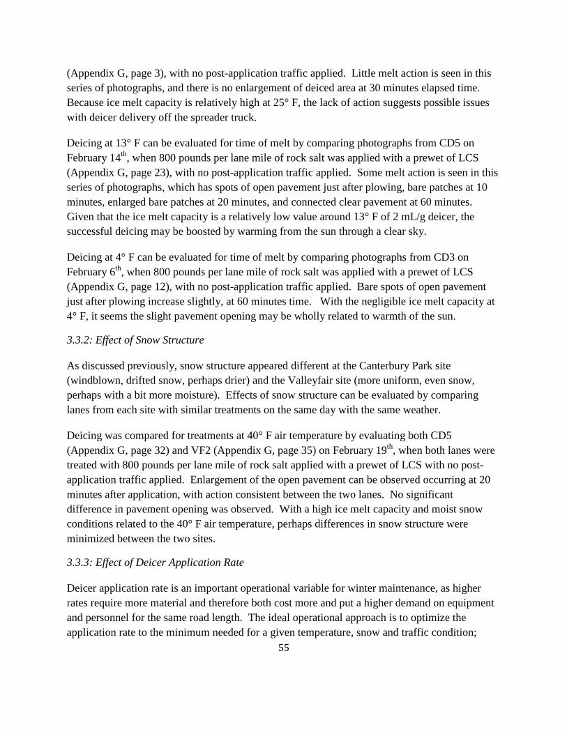
55
(Appendix G, page 3), with no post-application traffic applied. Little melt action is seen in this series of photographs, and there is no enlargement of deiced area at 30 minutes elapsed time. Because ice melt capacity is relatively high at 25° F, the lack of action suggests possible issues with deicer delivery off the spreader truck.
Deicing at 13° F can be evaluated for time of melt by comparing photographs from CD5 on February 14th, when 800 pounds per lane mile of rock salt was applied with a prewet of LCS (Appendix G, page 23), with no post-application traffic applied. Some melt action is seen in this series of photographs, which has spots of open pavement just after plowing, bare patches at 10 minutes, enlarged bare patches at 20 minutes, and connected clear pavement at 60 minutes. Given that the ice melt capacity is a relatively low value around 13° F of 2 mL/g deicer, the successful deicing may be boosted by warming from the sun through a clear sky.
Deicing at 4° F can be evaluated for time of melt by comparing photographs from CD3 on February 6th, when 800 pounds per lane mile of rock salt was applied with a prewet of LCS (Appendix G, page 12), with no post-application traffic applied. Bare spots of open pavement just after plowing increase slightly, at 60 minutes time. With the negligible ice melt capacity at 4° F, it seems the slight pavement opening may be wholly related to warmth of the sun.
3.3.2: Effect of Snow Structure
As discussed previously, snow structure appeared different at the Canterbury Park site (windblown, drifted snow, perhaps drier) and the Valleyfair site (more uniform, even snow, perhaps with a bit more moisture). Effects of snow structure can be evaluated by comparing lanes from each site with similar treatments on the same day with the same weather.
Deicing was compared for treatments at 40° F air temperature by evaluating both CD5 (Appendix G, page 32) and VF2 (Appendix G, page 35) on February 19th, when both lanes were treated with 800 pounds per lane mile of rock salt applied with a prewet of LCS with no post-application traffic applied. Enlargement of the open pavement can be observed occurring at 20 minutes after application, with action consistent between the two lanes. No significant difference in pavement opening was observed. With a high ice melt capacity and moist snow conditions related to the 40° F air temperature, perhaps differences in snow structure were minimized between the two sites.
3.3.3: Effect of Deicer Application Rate
Deicer application rate is an important operational variable for winter maintenance, as higher rates require more material and therefore both cost more and put a higher demand on equipment and personnel for the same road length. The ideal operational approach is to optimize the application rate to the minimum needed for a given temperature, snow and traffic condition;

56
however optimization can be quite difficult because there are so many variables associated with roadway conditions.
The experimental approach to evaluate deicer rate on this project was to apply deicer at different rates on pavement lanes under the same weather and traffic condition. MnDOT maintenance personnel described to researchers that 100 pounds per lane mile was spread most anytime a plow truck was traveling during the winter, such as out on patrol. 200 pounds per lane mile was spread when ice was sporadic, 400 pounds per lane mile was spread when ice was continuous, and 800 pounds per lane mile was spread when ice was heavy or there was high risk of ice formation. This project focused on 200, 400 and 800 pounds per lane mile as factor levels, for comparison.
Deicer application rate at 25° F can be evaluated by comparing photographs from CD1, CD2 and CD3 on January 29th, when 200, 400 and 800 pounds per lane mile, respectively, of rock salt was applied with a prewet of LCS (Appendix G, pages 1, 2 and 3), with no post-application traffic applied. As there was a failed camera for time-lapse photographs associated with CD1, hand held (Nikon) camera photographs have been assembled for CD1, CD2 and CD3 taken on January 29th in Appendix H, which also provides an opportunity for additional evaluation.
As discussed previously for the evaluation of time and temperature, the time-lapse photographs for the 800 pounds per lane mile treatment of CD 3 shows little melt action, and there is no enlargement of deiced area at 30 minutes elapsed time. Because ice melt capacity is relatively high at 25° F, the lack of action suggests possible issues with deicer delivery off the spreader truck. Conversely, the time-lapse photographs for the 400 pounds per lane mile treatment of CD2 show a much greater ice melt, though perhaps an excess amount for the application rate. Examination of Figure H in Appendix H shows an isolated patch of highly deiced pavement that appears to be associated with an over delivery of deicer.
Comparison of the hand held camera photographs of Appendix H across the three application rates shows increasing melted areas and cleared pavement with the increase of rate from 200 to 400 pounds per lane mile. However, the amount of cleared pavement with 800 pounds per lane mile does not seem appreciably more than with 400 pounds per lane mile. For the 25° F temperature, it seems 400 pounds per lane mile would be sufficient, and 800 pounds per lane mile an excessive and unneeded increase in application.
In contrast, deicer application rate may be evaluated for 4° F by comparing photographs from CD1, CD2 and CD3 on February 6th, when 200, 400 and 800 pounds per lane mile, respectively, of rock salt was applied with a prewet of LCS (Appendix G, pages 10, 11 and 12), with no post-application traffic applied (same conditions as the previous evaluation except for the temperature being 4° F instead of 25° F). Hand held camera photographs were also prepared for these lanes

57
and are presented as Appendix I. As the ice melt capacity is very low, near zero, for 4° F, little action was expected, and the photographs all indicate very little melt with one exception: the 800 pounds per lane mile treatment seems to have caused some deicing, as shown in photographs S and T of Appendix I. Given that the day was clear and sunny, perhaps the increased application rate helped with solar warming to create the deicing observed.
3.3.4: Effect of Traffic
MnDOT maintenance personnel had reported their anecdotal observations that traffic, particularly truck traffic, could make a substantial improvement in roadway deicing. The hypothesis is that the vehicle pressure creates a closer physical contact between the deicer grain and the ice, particularly if the ice is not fully consolidated, i.e., lightly packed snow. Also, truck traffic might create better deicing because truck tires are often inflated to 90 psi, rather than the 35psi typical of passenger vehicles, resulting in greater vehicle pressure.
To evaluate the effect of traffic in this project, lanes were designated for no traffic, car traffic or truck traffic and compared under similar deicer application and during the same weather. Traffic was applied through 5 passes of either a passenger vehicle (Ford Windstar minivan or Toyota Rav 4 utility vehicle) or a plow/deicer spreading truck typically loaded with about 5 ton of deicer. Two different days with different temperatures were evaluated: February 19th with an air temperature of 40° F and February 14th with an air temperature of 13° F. On both days, 800 pounds per lane mile of rock salt was applied with a prewet of LCS to all lanes tested for traffic evaluation. Lane CD2 had no post-application traffic, CD1 had five passes of a passenger vehicle, and CD 3 had five passes of a truck. Additional comparison could be made for each day using VF2 with five passes of a passenger vehicle and VF1 with five passes of a truck.
Comparing traffic effects at an air temperature of 40° F for the Canterbury Park lanes (Appendix G, pages 29, 28 and 30 for no, passenger vehicle and truck traffic, respectively), it appears that lanes open up at similar rates. At 20 minutes, each of the traffic conditions showed wheel line open pavement. At 30 minutes, each of the traffic conditions was broadly open where the deicer had been applied, while at 60 minutes the pavement was widely open.
Similar results were seen for the same 40° F temperature at the Valleyfair lanes (Appendix G, pages 35 and 34 for passenger vehicle and truck traffic, respectively), though the width of the open pavement was not as great. It can be seen in the photographs that the slope of each Valleyfair lane is to the vehicle’s left, which may have caused the salt brine to have migrated off the travel way rather than across the lane towards the vehicle’s right, as the deicer was distributed from the truck’s left side. The relatively thinner area of melt for Valleyfair lanes when compared to Canterbury Park lanes is therefore considered an artifact of the test conditions, and not representative of deicer applied to a normally crowned roadway.

58
Comparing traffic effects at an air temperature of 13° F for the Canterbury Park lanes (Appendix G, pages 20, 19 and 21 for no, passenger vehicle and truck traffic, respectively), differences were more significant. With no traffic, there is little change observed with time in the ice and snow on the treated lane. With car traffic, there is modest improvement in open pavement, primarily occurring in the 30 to 60 min time range. With truck traffic, there is substantial melting occurring between 10 and 20 min after application, beginning with the opening of the left wheel line (the location of the deicer distribution point) then widening to about half the lane. Interesting to compare is that the right wheel line, away from the deicer distribution point, does not become open pavement, suggesting that it is the combination of deicer and tire pressure that causes the melt, not the tire pressure alone.
Although not directly comparable, a similar result can be seen for lane CD6 for the same day, which had 800 pounds per lane mile rock salt applied but with no prewet, then truck traffic applied (Appendix G, pages 24). The left wheel lane opens but not the right, again in the time frame of 10 to 20 min after application.
Similar results of truck traffic providing a more effective boost in melt were seen for the same 13° F temperature at the Valleyfair lanes (Appendix G, pages 26 and 25 for passenger vehicle and truck traffic, respectively).
3.3.5: Effect of Prewet
Prewet is reportedly applied to solid deicer to bring about a quicker initiation of melting and to hold the deicer onto the roadway surface during windy conditions. Prewet was evaluated during this project to verify the reported behavior.
Lanes were treated on a single day (same weather) with similar deicer application and had the same traffic, but alternated between having prewet added to the deicer or having no prewet. Two different application rates were used at four different temperatures (different days) were evaluated:
• 400 pounds per lane mile of rock salt with a prewet (when used) of LCS on February 4th with an air temperature of 4° F (Table 13) and January 29th with an air temperature of 25° F (Table 14); and,
• 800 pounds per lane mile of rock salt with a prewet (when used) of LCS on February 19th with an air temperature of 40° F (Table 15) and February 14th with an air temperature of 13° F (Table 16).
Observations of the difference made by prewet as well as the difference made by traffic are included in each table.
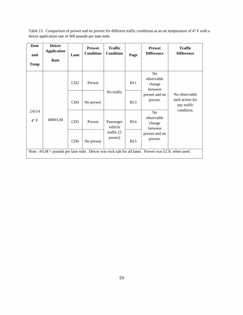
59
Table 13. Comparison of prewet and no prewet for different traffic conditions at an air temperature of 4° F with a deicer application rate of 400 pounds per lane mile.
Date
and
Temp
Deicer Application
Rate
Lane
Prewet Condition
Traffic Condition
Page
Prewet Difference
Traffic Difference
2/6/14
4° F
400#/LM
CD2
Prewet
No traffic
B11
No observable
change between
prewet and no prewet.
No observable melt action for
any traffic condition.
CD4
No prewet
B13
CD5
Prewet
Passenger vehicle
traffic (5 passes)
B14
No observable
change between
prewet and no prewet.
CD6
No prewet
B15
Note: #/LM = pounds per lane mile. Deicer was rock salt for all lanes. Prewet was LCS, when used.

60
Table 14. Comparison of prewet and no prewet for different traffic conditions at an air temperature of 25° F with a deicer application rate of 400 pounds per lane mile.
Date
and
Temp
Deicer Application
Rate
Lane
Prewet Condition
Traffic Condition
Page
Prewet Difference
Traffic Difference
1/29/14
25° F
400#/LM
CD2
Prewet
No traffic
B2
No observable
change between
prewet and no prewet.
Little observable melt action for
any traffic condition
CD4
No prewet
B4
CD5
Prewet
Passenger vehicle
traffic (5 passes)
B5
Slight improvementaround spots plowed bare with prewet
CD6
No prewet
B6
Note: #/LM = pounds per lane mile. Deicer was rock salt for all lanes. Prewet was LCS, when used.

61
Table 15. Comparison of prewet and no prewet for different traffic conditions at an air temperature of 13° F with a deicer application rate of 800 pounds per lane mile.
Date
and
Temp
Deicer Application
Rate
Lane
Prewet Condition
Traffic Condition
Page
Prewet Difference
Traffic Difference
2/14/14
13° F
800#/LM
CD5
Prewet
No traffic
B23 Prewet or no prewet works equally well.
Truck traffic greatly improves deicing, opening lane quicker and
wider. 10 min for wheel line, 20 min for broad melt, 60
min for whole lane.
CD2
No prewet
B20
CD1
Prewet
Passenger vehicle
traffic (5 passes)
B19 Prewet or no prewet works equally well.
CD4
No prewet
B22
CD3
Prewet
Truck traffic (5 passes)
B21 Prewet or no prewet works equally well.
CD6
No prewet
B24
Note: #/LM = pounds per lane mile. Deicer was rock salt for all lanes. Prewet was LCS, when used.

62
Table 16. Comparison of prewet and no prewet for different traffic conditions at an air temperature of 40°F with a deicer application rate of 800 pounds per lane mile.
Date
and
Temp
Deicer Application
Rate
Lane
Prewet Condition
Traffic Condition
Page
Prewet Difference
Traffic Difference
2/19/14
40° F
800#/LM
CD5
Prewet
No traffic
B32 Prewet or no prewet works equally well.
Truck traffic greatly improves deicing, opening lane quicker and
wider. 10 min for wheel line, 20 min for broad melt, 30
min for whole lane.
CD2
No prewet
B29
CD1
Prewet
Passenger vehicle
traffic (5 passes)
B28 Prewet or no prewet works equally well.
CD4
No prewet
B31
CD3
Prewet
Truck traffic (5 passes)
B30 Prewet or no prewet works equally well.
CD6
No prewet
B33
Note: #/LM = pounds per lane mile. Deicer was rock salt for all lanes. Prewet was LCS, when used.
Prewet caused no observable difference in melt performance at any of the conditions tested. This observation may be a result of using photographs at a 10-minute increment, as it may be possible that melt differences could be occurring quicker than the time increment. However, the effect of truck traffic previously discussed was fully evidenced for the 13 and 40° F air temperatures that had 800 pounds per lane mile application rate. The lack of effect for truck traffic at the 4 and 25° F air temperatures may be related to the 400 pounds per lane mile application rate, particularly for the 25° F air temperatures at which ice melt capacity is higher, in that the 400 pound per lane mile application rate may not be sufficient to cause observable melt for the pavement and traffic conditions of this work. While maintenance personnel report that 400 pounds per lane mile is an acceptable application rate for roadways, perhaps with only five

63
passes of a vehicle the deicer mixing is not enough for the unconsolidated (snowy) materials of the project sites.
3.3.6: Effect of Wind and Sun or Overcast
Wind and sun or overcast have been suggested by winter maintenance personnel to have significant effects on deicing performance. Wind can remove deicer from the roadway surface, or cool the surface and create conditions conducive for refreeze. Wind can create drift structure for the snow, areas that alternate between thick and thin, and wind may dry moisture out of icy materials. Sun can warm a roadway, particularly asphalt, exploiting the non-reflective surface of the pavement and enlarging open patches. Sun can also reduce the thickness of less-consolidated (snowy) ice, increasing the moisture content of the snowy material that remains.
For the current project, no same day/same temperature evaluations of wind and sun or overcast were made. It is recommended that wind and sun or overcast be evaluated in the future.
3.4: Conclusions
A deicing test facility was set up and procedures established. Six and three parallel 1000-foot long lanes were created at two facilities offering a range of snow conditions. Time-lapse photography worked well to document melting conditions, at least during daylight hours. Ice base creation procedures were developed but remain somewhat difficult to do in winter conditions without a ready supply of cold water.
Deicing results followed the expectations developed in laboratory studies for temperature, with warmer temperatures providing more melt from the deicer. Little melt was observed below about 10° F unless sunlight provided warming. Additional work is needed to evaluate deicing behaviors when faced with changing temperatures, i.e., formation of refreeze when temperatures drop but the roadway is still wet with brine, activation of deicing when temperatures rise from a cold application temperature, etc. Time of the melting process did not appreciably change with temperature, and any changes noted may be more related to the increased ice melt capacity with increased temperature. However, additional work could be done to fine tune the melt time characteristics, perhaps with closer photography at more rapid increments.
The effect of snow structure on melt performance was inconclusive but was done on a relatively warm day when deicing was highly effective for all conditions. Future evaluation should be done for temperatures in the 15 to 25° F range, perhaps including measurements of snow moisture and sunlight.
Application rate was observed to have the best results at 800 pounds per lane mile, with best being defined as widest melt area. Melt area size is important to this study, as wider effects are

64
easier to discern and compare. However, it is recognized that while melt area is important, cost efficiency and reduced deicer usage may also be important winter maintenance requirements. Finding the optimum balance between deicer performance level, cost and deicer usage requires many more inputs than considered in this research project, and an optimum balance evaluation would require consideration of specific factors for a given situation. Therefore, it must be concluded that application rate effects deicing performance level, as expected, and is a factor that must be designed around in winter maintenance operations.
Perhaps more importantly, snow should be compacted (consolidated), perhaps by truck traffic, prior to testing in future evaluations. Application rate may need to be reconsidered when the majority of the ice is higher moisture content, consolidated material rather than snow-like unconsolidated material.
The need for replication of test conditions in evaluations within deicer research was suggested by the results when camera failure, camera malfunction, or spreader variation was observed. Having second lanes with replicated test conditions would help limit impacts of unexpected equipment issues and provide much higher strength of observation and evaluation.
No significant difference was observed in deicer performance by whether prewet was used or not. Benefits reported by maintenance personnel of better roadway adherence during windy conditions and quicker initiation of melt were not observed during this study, and may warrant further evaluation if deemed important.
Traffic, specifically truck traffic, was found to cause a significant improvement in deicer performance, with both wider and quicker melt occurring. The interaction of tire pressure and deicer was clearly observed to create the improved melting, as compared to the effect of the tire pressure alone.

65
Chapter 4: Plow Effectiveness Study
This study aims to characterize and define the factors influenced by plow effectiveness by developing and using an outdoor pavement facility with nine 1000-ft long lanes for treatment areas, separated to prevent incidental cross-treatment, located in Shakopee, Minnesota, at two proximal locations. The length of plowed areas was set to provide sufficient room for normal highway operating speeds of plow trucks. Time-lapse cameras were placed sufficiently close to treatment areas to observe and document post-plow pavement in high definition. Plow trucks were supplied by MnDOT Metro District on non-storm days. Factors evaluated included: truck speed, snow structure between days/different storm composition, and snow structure differing by field site geography.
4.1: Test Method
4.1.1: Method Design
For this evaluation of plow effectiveness and contributing factors, pavement lanes were set up and defined where plowing could be done without actual traffic such that experimental approaches could be tried out and compared without potential for compromising public safety. Lane lengths of 900 to 1000 ft long were defined, plus additional space for turning, so that plow trucks could reach and maintain highway speeds of approximately 30 mph. Time-lapse and hand held camera photographs were used to augment observation notes and to document the effectiveness of plowing techniques for the different snow conditions.
Plowing approaches were compared both within the conditions of a given day and under different weather conditions between days. Actual snow conditions were used. MnDOT plow trucks were used on non-storm days to closely model actual efforts without significantly diverting equipment necessary for actual road maintenance during storms.
4.1.2: Field Sites
Shakopee was targeted for project field sites to provide locations accessible both to researchers from Minnesota State, Mankato and maintenance personnel of MnDOT Metro District, with potential for additional access by maintenance personnel of other nearby MnDOT Districts. Pavement lanes were set up in Shakopee at two locations with large parking lots not typically used during winter months:
• Canterbury Park, 1100 Canterbury Road; in the overflow parking lot on the north side of the facility, approximately 0.25 mile south of 4th Avenue East and 0.5 mile west of Canterbury Road South (Figure 24a).

66
• Valleyfair, One Valleyfair Drive; in the back (north) parking lot on the north east corner of the facility, located north of TH 101 about 2.5 miles west of US 169 (Figure 24b).
a) Canterbury Park
b) Valleyfair
Figure 24. Pavement areas with snow cover prior to plowing.

67
Access agreements were negotiated and agreed upon during early December, 2013. Prior to a lasting snowfall, researchers with support from MnDOT Metro District maintenance staff performed pavement surveys to locate and document surface discontinuities (Figure 25) that could either interfere with or be damaged by plowing. Test lanes were configured to avoid such discontinuities.
a) Drainage structure at Canterbury Park b) Transverse drainage gutter at Valleyfair
sides of individual lanes. Pin flags were anchored through 6 in x 3 in x 2 in “sewer” (hollow core) bricks to 8 in x 8 in x ¾ in wooden plates and stabilized by 1 ft lengths of ¾ in diameter Schedule 40 PVC pipe. Anchoring was done to prevent penetration of the pavement by the flags yet maintain the flags in spite of winter winds.
Initial lane cuts were made December 18th (Figure 26); afterwards flags were reset on measured locations to represent 100-ft stationing along both sides of each lane (Figure 27).
Lane marking was done with pin flags of various colors; colors were assigned to designate the
Figure 25. Pavement discontinuities, noted prior to snowfall.
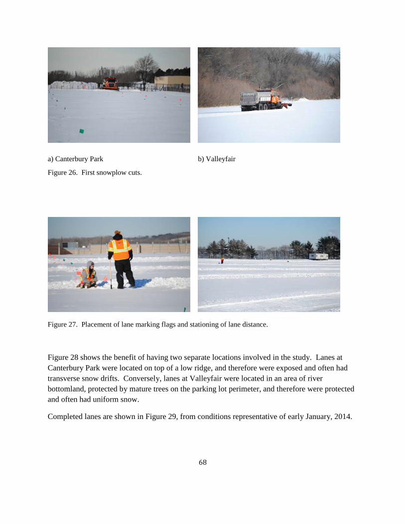
68
a) Canterbury Park b) Valleyfair
Figure 26. First snowplow cuts.
Figure 27. Placement of lane marking flags and stationing of lane distance.
Figure 28 shows the benefit of having two separate locations involved in the study. Lanes at Canterbury Park were located on top of a low ridge, and therefore were exposed and often had transverse snow drifts. Conversely, lanes at Valleyfair were located in an area of river bottomland, protected by mature trees on the parking lot perimeter, and therefore were protected and often had uniform snow.
Completed lanes are shown in Figure 29, from conditions representative of early January, 2014.

69
a) Canterbury Park February 13, 2014 showing wind effects and creation of drift structure.
b) Valleyfair January 8, 2014 showing uniformity of conditions created by river bottomland and tree protection.
Figure 28. Comparison of conditions possible between field sites.

70
a) Canterbury Park
b) Valleyfair
Figure 29. Completed lanes.

71
4.1.3: Weather Measurement
A Kestrel 4000 handheld weather station (Nielsen-Kellerman, Boothwyn, PA), capable of determining temperature, relative humidity, dew point and wind speed, was used to determine conditions during field operations (Figure 30a). A dial thermometer (Figure 30b) was used for illustration and photographic documentation, but was not considered sufficiently accurate to represent field conditions. Weather measurements were augmented with documentation from a paid subscription to WeatherSpark.com, used for interpreting National Weather Service data obtained from Flying Cloud Airport, Eden Prairie, Minnesota, approximately 2 miles north of either field site.
a) Handheld weather station. b) Dial thermometer.
Figure 30. Weather monitoring tools.
4.1.4: Cameras and Photography
Field conditions were documented through photography using two different camera systems. Handheld, high resolution photographs were taken using a Nikon D3000 camera with a 55-200 mm telephoto lens, occasionally alternating with a 20-55 mm wide angle lens.
Time-lapse photographs were taken using Stealth Calm Core 3 time-lapse (game scouting) cameras (Figure 31) (Stealth Cam, LLC, Grand Prairie, TX). Time-lapse cameras were pole mounted at approximately a 6-ft height, with poles attached to wooden bases. Wooden bases were set aside once windrows built up along test lanes, as poles were directly inserted into windrows for support.

72
Typically, time-lapse cameras were installed at lane station 1+00 for each lane, meaning 100 ft from the start of the lane, oriented in the direction of the plow and deicer truck movement. Time increments of 1 minute were typically used. Date and time stamps were made on time-lapse photographs, though all photographs had file origination information that could provide time of capture for verification, if needed.
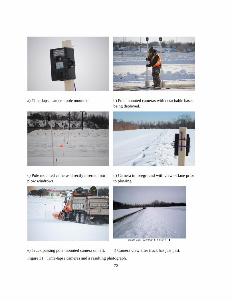
73
a) Time-lapse camera, pole mounted. b) Pole mounted cameras with detachable bases being deployed.
c) Pole mounted cameras directly inserted into plow windrows.
d) Camera in foreground with view of lane prior to plowing.
e) Truck passing pole mounted camera on left. f) Camera view after truck has just past.
Figure 31. Time-lapse cameras and a resulting photograph.

74
4.1.5: Plow and Deicer Spreading Operations
Plowing and deicer spreading (distribution) were done by maintenance personnel from MnDOT Metro District using equipment from the Chaska Truck Station. Typical equipment was a 2006 Sterling tandem axle, automatic transmission dump truck with front, right wing and underbody plows (Figure 32a). Side mounted (saddle) tanks were used to carry brine materials used for prewetting granular deicer (Figure 32b). A transverse auger was mounted in the rear of the dump body to feed deicer either to the left or right chute. Granular deicer was maintained in contact with the auger by frequent plow body raising such that the granular deicer would shift to the back of the plow body where the auger was located. Deicer would fall through the chute to a distributor (spinner) plate (Figure 32c). Prewet was poured via gravity onto the granular deicer when on the distributor plate (Figure 32d). The distributor plate rotated when the truck was in forward motion, spreading deicer rather than having a straight drop (Figure 33).
a) MnDOT tandem axle dump truck with front and right wing plows engaged.
b) MnDOT truck with saddle tanks for prewet fluid.
c) Salt distributor behind left rear wheel (not in motion/not being fed deicer at time of photo).
d) Prewet flow onto salt distributor (not in motion/not being fed deicer at time of photo).
Figure 32. Plow and deicer equipment on a MnDOT truck used for this study.
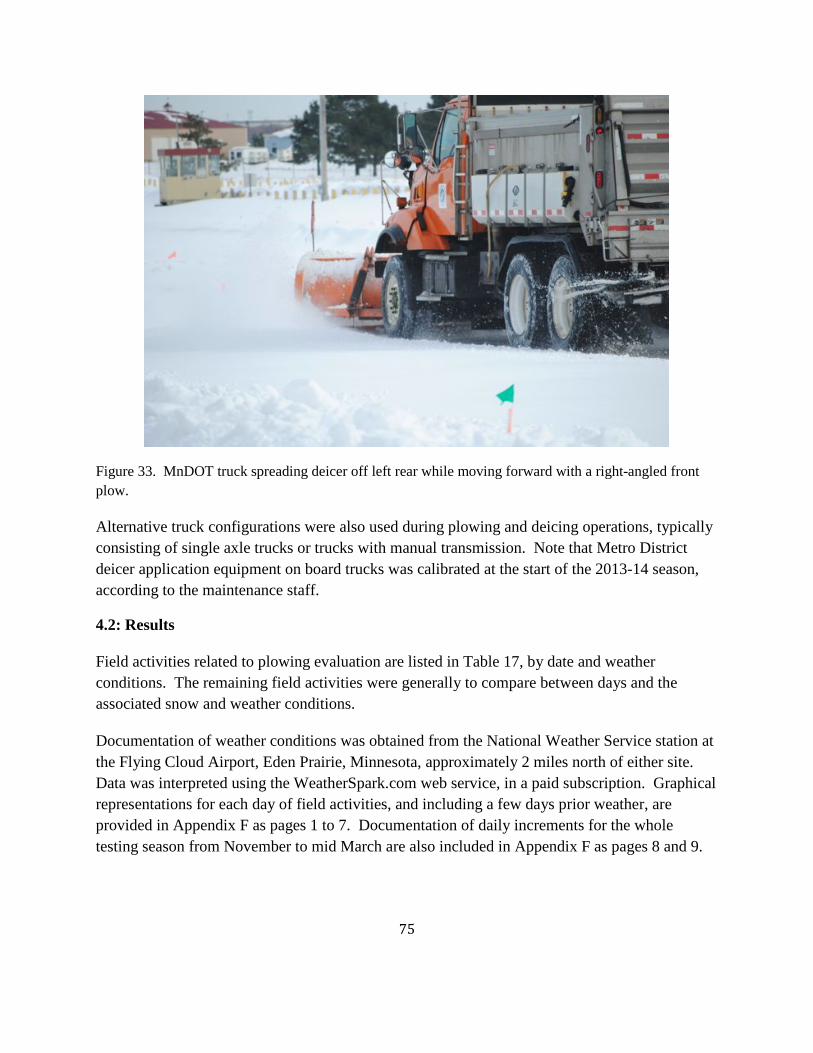
75
Figure 33. MnDOT truck spreading deicer off left rear while moving forward with a right-angled front plow.
Alternative truck configurations were also used during plowing and deicing operations, typically consisting of single axle trucks or trucks with manual transmission. Note that Metro District deicer application equipment on board trucks was calibrated at the start of the 2013-14 season, according to the maintenance staff.
4.2: Results
Field activities related to plowing evaluation are listed in Table 17, by date and weather conditions. The remaining field activities were generally to compare between days and the associated snow and weather conditions.
Documentation of weather conditions was obtained from the National Weather Service station at the Flying Cloud Airport, Eden Prairie, Minnesota, approximately 2 miles north of either site. Data was interpreted using the WeatherSpark.com web service, in a paid subscription. Graphical representations for each day of field activities, and including a few days prior weather, are provided in Appendix F as pages 1 to 7. Documentation of daily increments for the whole testing season from November to mid March are also included in Appendix F as pages 8 and 9.

76
Table 17. Plowing activities by date, weather and snow conditions.
Date Weather Snow Plowing Activities (Truck)
12/18/2013 5°F, clear and
sunny
wind 0-3 mph
CD: 3 – 6 inches crusty, drifted snow
VF: 4 – 6 inches, uniform snow
Evaluation of effects from truck speed: 5, 10, 15, and 20 mph.
Truck 3153 tandem axel with automatic transmission (AVL 206552)
1/8/2014 -5°F, clear and
sunny
wind 5 mph
CD: 2 – 3 inches, drifts to 6 inches, dry
VF: No plowing done
Slow and steady 10 mph, evaluation of plowing drift structure.
Truck tandem axel with manual transmission (AVL 200043)
1/10/2014 28°F, overcast
wind 10-15 mph
CD: No plowing done
VF: 2 – 3 inches, drifts to 6 inches, dry
Plow evaluation not made.
Truck 3153 tandem axel with automatic transmission (AVL 206552)
1/29/2014 25°F, clear and
sunny
wind 5-15 mph
CD: 1 – 2 inches thin, dry snow with small drifts
VF: 2– 3 inches, dry snow
Plowing fast at 30 mph.
Truck 3153 tandem axel with automatic transmission (AVL 206552)
2/6/2014 4°F, clear and
sunny
wind 8-12 mph
CD: 2 – 3 inches slightly moist snow
VF: 2– 3 inches, slightly moist snow
Plowing at medium speed of perhaps 20 mph.
Truck 3153 tandem axel with automatic transmission (AVL 206552)
2/14/2014 13°F, clear and
sunny
wind 8-12 mph
CD: ½ – 1 inch thin, dry snow with bare spots
VF: 1– 2 inches, dry snow, uniform
Plowing at medium speed of perhaps 20 mph, evaluation of surface scraping
of thin, windblown snow.
Truck (unknown number) single axel
2/19/2014
40°F, clear and sunny
wind 0-3 mph
CD: 2 – 3 inches moist snow
VF: 2– 3 inches moist snow
Plowing at medium speed of perhaps 20 mph, evaluation of plowing
“thicker” consistency snow.
Truck 3153 tandem axel with automatic transmission (AVL 206552)
Note: There was insufficient snow cover before 12/3/2013 by which to plow and deice; there was insufficient cold as of 3/6/2014 to maintain snow cover until MnDOT plow and deicing trucks were available.
77
Hand held (Nikon) camera photography was used for plow effectiveness documentation, capturing photos in “rapid fire” or “burst” mode during plowing. Time-lapse photography was added during four field days (January 29th, February 6th, 14th and 19th) when plowing and deicing activities were done on over the full distance of a pavement lane.
Photographic documentation of each lane during plowing activity (Figure 34) is provided in summary form in Appendix K. Photographs are provided for times prior to plowing, three moments during plowing, immediately after plowing, and 10 minutes after plowing. Where noted, “camera malfunction” typically represents a camera that did not withstand the snow thrown by the passing plow; photographs of the lane were therefore not obtained until the camera was picked up and repositioned.
Photographs used in the summary forms of Appendix K for the times prior to plowing, immediately after plowing and 10 minutes after plowing were selected to illustrate snow and pavement conditions typical of either before or after plowing. Photographs of the moments during plowing were selected to illustrate dislodgement and casting of snow during the plow action.
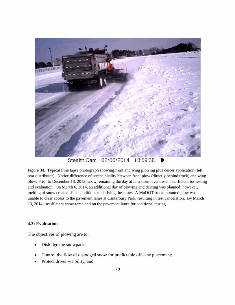
78
Figure 34. Typical time lapse photograph showing front and wing plowing plus deicer application (left rear distributor). Notice difference of scrape quality between front plow (directly behind truck) and wing plow. Prior to December 18, 2013, snow remaining the day after a storm event was insufficient for testing and evaluation. On March 6, 2014, an additional day of plowing and deicing was planned; however, melting of snow created slick conditions underlying the snow. A MnDOT truck mounted plow was unable to clear access to the pavement lanes at Canterbury Park, resulting in test cancelation. By March 13, 2014, insufficient snow remained on the pavement lanes for additional testing.
4.3: Evaluation
The objectives of plowing are to:
• Dislodge the snowpack;
• Control the flow of dislodged snow for predictable off-lane placement; • Protect driver visibility; and,

79
• Leave a roadway surface scraped bare or with a low amount of residual snow (likely to be removed using deicing techniques).
These objectives are best met with low equipment and labor cost, meaning effective snow removal in a single pass, preferably at speeds of around 25 to 30 mph typically recommended for highway plowing and deicing operations (speed selected to optimize safety and deicer application).
This study evaluates factors that can improve plowing performance in meeting these objectives. The energy required to move a given amount of snow (fuel efficiency) was not evaluated in this study, but would also relate to efficiency of operation.
Evaluation of plowing results was made for selected factors using time-lapse photography of treated lanes, primarily represented by the photographs presented in Appendix K and augmented by field observations during the plowing efforts.
4.3.1: Comparison of Plow Scrape Quality Across Single Site
Two different days were evaluated for differences in plow performance across snow and weather conditions at a single site. Results from Canterbury Park lanes CD1 to CD 6 were evaluated for February 6th, a colder day with 2 – 3 inches of snow (Figure 35), and for February 19th, a warmer day also with 2 – 3 inches of snow (Figure 36). Plow speeds were 20 mph on both days using the same truck.
No significant differences were observed in plowing results across the site from CD1 to CD6 on either day. The front plow scraped to ~ ¼th inch residual snow on average, with a moderate amount of pavement bared. The wing plow scraped to ~ ½ inch residual snow on average, with no pavement bared. No significant differences were observed between the days, in spite of the temperature difference (air temperatures of 4°F versus 40°F).
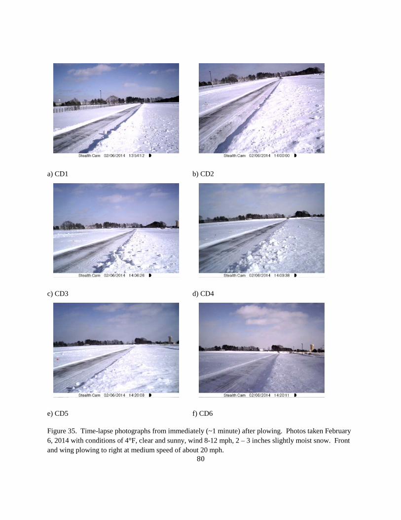
80
a) CD1 b) CD2
c) CD3 d) CD4
e) CD5 f) CD6
Figure 35. Time-lapse photographs from immediately (~1 minute) after plowing. Photos taken February 6, 2014 with conditions of 4°F, clear and sunny, wind 8-12 mph, 2 – 3 inches slightly moist snow. Front and wing plowing to right at medium speed of about 20 mph.

81
a) CD1 b) CD2
c) CD3 d) CD4
e) CD5 f) CD6
Figure 36. Time-lapse photographs from immediately (~1 minute) after plowing (except CD 1 and CD 2 are from 11 and 6 minutes after plowing, respectively). Photos taken February 19, 2014 with conditions of 40°F, clear and sunny, wind 0 – 3 mph, 2 – 3 inches moist snow. Front and wing plowing to right at medium speed of about 20 mph.

82
4.3.2: Comparison of Plow Scrape Quality Across Single Site
Comparison was also made between the two sites with the same truck, speed and weather but with different pavements and perhaps slightly different snow conditions. Results from Canterbury Park lanes CD 1, CD 3 and CD 5 were compared to results from Valleyfair lanes VF 1, VF 2 and VF 3 on a single day for each of the same two days previously evaluated: February 6th, a colder day with 2 – 3 inches of snow (Figure 37), and for February 19th, a warmer day also with 2 – 3 inches of snow (Figure 38). Plow speeds were 20 mph on both days using the same truck.
Again, no significant differences were observed in plowing results between the sites on either day. The front plow scraped to ~ ¼th inch residual snow on average, with a moderate amount of pavement bared. The wing plow scraped to ~ ½ inch residual snow on average, with no pavement bared. No significant differences were observed between the days, in spite of the temperature difference (air temperatures of 4°F versus 40°F).
4.3.3: Evaluation of Plow Speed Effects on Dislodged Snow Removal
Evaluation was made of plow speed effects on the movement and removal of dislodged snow using different speeds on different lanes with the same truck, snow and weather conditions. Results from December 18th, a colder day with 3 – 6 inches of crusty, drifted snow, were evaluated for Canterbury Park lanes CD1 to CD 6 (Figure 39). Plow speeds were varied from 5 to 20 mph using the same truck.
As expected, snow rises higher in the curvature of the plow in response to higher speeds. Higher speeds create a broader spray off the plow ends, with an accompanying greater distribution distance of the dislodge snow.
No evaluation of pavement scrape quality in response to speed was made at this time, as time lapse cameras were not yet deployed or installed.
Different speeds were also compared across different days and the particular snow conditions (Figure 40), comparing three days with three different speeds:
• 10 mph on January 8th, -5°F, with 2 – 3 inches, drifts to 6 inches, dry snow. • 20 mph on February 6th, 4°F, with 2 – 3 inches, slightly moist snow. • 30 mph on January 29th, 25°F, with 1 – 2 inches, dry snow with small drifts.
Two lanes (CD 2 and CD 4) at Canterbury Park were selected for evaluation, based on the representativeness of the lanes.

83
Even with different snow and temperature conditions, the evaluation of speed provides the same conclusion as before: snow rises higher in the curvature of the plow in response to higher speeds, and higher speeds create a broader spray off the plow ends, with an accompanying greater distribution distance of the dislodged snow.

84
a) CD1 b) VF1
c) CD3 d) VF2
e) CD5 f) VF3
Figure 37. Comparison between Canterbury Park (CD Lanes) and Valleyfair (VF Lanes) sites using time-lapse photographs from immediately (~1 minute) after plowing. Photos taken February 6, 2014 with conditions of 4°F, clear and sunny, wind 8-12 mph, 2 – 3 inches slightly moist snow. Front and wing plowing to right at medium speed of about 20 mph. Photos a, c, and e repeated from Figure 35.

85
a) CD1 b) VF1
c) CD3 d) VF2
e) CD5 f) VF3
Figure 38. Comparison between Canterbury Park (CD Lanes) and Valleyfair (VF Lanes) sites using time-lapse photographs from immediately (~1 minute) after plowing (except CD 1 and VF3 are from 11 and 6 minutes after plowing, respectively). Photos taken February 19, 2014 with conditions of 40°F, clear and sunny, wind 0 – 3 mph, 2 – 3 inches moist snow. Front and wing plowing to right at medium speed of about 20 mph. Photos a, c, and e repeated from Figure 35.

86
a) CD1 at 5 mph. b) CD2 at 10 mph.
c) CD3 at 15 mph. d) CD4 at 20 mph, front plow angled left.
e) CD5 at 20 mph. f) CD6 at 20 mph.
Figure 39. Comparison between different plowing speeds within similar snow and weather conditions of a single site on a single day. Photos taken December 18, 2013 with conditions of 5°F, clear and sunny, wind 0 – 3 mph, 3 – 6 inches crusty, drifted snow. Front and wing plowing to right excepted where noted.

87
a) CD2, January 8th, -5°F, 2 – 3 inches, drifts to 6 inches, dry snow. 10 mph.
b) CD4, January 8th, -5°F, 2 – 3 inches, drifts to 6 inches, dry snow. 10 mph.
c) CD2, February 6th, 4°F, 2 – 3 inches, slightly moist snow. 20 mph.
d) CD4, February 6th, 4°F, 2 – 3 inches, slightly moist snow. 20 mph.
e) CD2, January 29th, 25°F, 1 – 2 inches, dry snow with small drifts. 30 mph.
f) CD4, January 29th, 25°F, 1 – 2 inches, dry snow with small drifts. 30 mph.
Figure 40. Comparison of plowing on different speeds during different snow and weather conditions of two lanes from a single site on different days. Left photos all Canterbury Park Lane 2 (CD2). Right photos all Canterbury Park Lane 4 (CD4).

88
4.4: Conclusions
A plowing test facility was set up and procedures established. Six and three parallel 1000-foot long lanes were created at two facilities offering a range of snow conditions. Time-lapse photography worked well to document snow clearing conditions, at least during daylight hours.
Similar results were obtained across six different lanes at one facility, suggesting strong replication of performance. Results appeared consistent over the length of the lanes, based on the photographs. Similar results were also seen when plowing was compared between two sites with slightly different snow conditions, suggesting uniformity in results from a single truck, plow and driver combination.
Because of the severe conditions during the winter of 2013-14, multiple plow combinations were not available on a single day of testing. Therefore, equipment variations were not able to be tested. It is hoped that future evaluations will be done for cutting edge/blade, plow shape, plow material and truck variations.
Plowing results followed expectations for differences in speed, in that snow rises higher in the curvature of the plow in response to higher speeds, and higher speeds create a broader spray off the plow ends, with an accompanying greater distribution distance of the dislodged snow.
Perhaps as importantly, snow should be compacted (consolidated), perhaps by truck traffic, prior to testing in future evaluations. Application rate may need to be reconsidered when the majority of the ice is higher moisture content, consolidated material rather than snow-like unconsolidated material.

89
Chapter 5: Pavement Study
One technique of winter maintenance operations that has shown great promise is anti-icing, the pre-storm placement of deicer brine to clear pavement done to limit or prevent formation of icing on a roadway. Whether due to wind blown snow, ice fog, freezing rain, or simply wet snow becoming packed (Figure 41), anti-icing has been found to reduce formation and build up. However, winter maintenance operations have often found it difficult to mobilize the anti-icing application trucks, either because of labor shortages prior to a storm (resting crews before potential long shifts) or limited procurement of the anti-icing brine application equipment (Figure 42). Application of sodium chloride (rock salt) brine at typical rates between 10 and 30 gallons per lane mile (gal/LM) also provides a significant deicer material savings, as with a brine saturation of 23% concentration this rate calculates to 20 to 60 lb/LM, about 1/20th of the typical deicer application rate during a snow event.
However, anti-icing and deicing operations could be negatively affected by the roadway wetness as traffic removes salt through splash and spray as well as run off. Blomqvist, et al (2011) observed:
Road surface wetness, as shown from the wheel tracks, related positively to the rate of residual salt loss. The wetter the surface, the faster the salt left the wheel tracks. On a wet road surface, the salt in the wheel tracks was almost gone after only a couple of hundred vehicles had traveled across the surface, whereas on a moist road surface, it would take a couple of thousand vehicles to reach the same result.
This study aims to characterize and define the pavement aspects of these factors by performing laboratory tests of deicer persistence using different pavement types. Different deicer/anti icer chemicals were evaluated in response to application of artificial precipitation. Pavements were prepared by application of deicer chemical in either brine or solid form, dried or burnished to replicate service conditions, then chilled. Measurements of chloride content were made to see how long the deicer chemical stuck to the pavement in relationship to the precipitation amount.
This report represents the work done under Task 4 of MnDOT Agreement 02829, Salt Brine Blending to Optimize Deicing and Anti-Icing Performance and Cost Effectiveness Phase II. This work was performed by Minnesota State University (MSU), Mankato in the Environmental Engineering laboratory, as part of the Center for Transportation Research and Implementation.
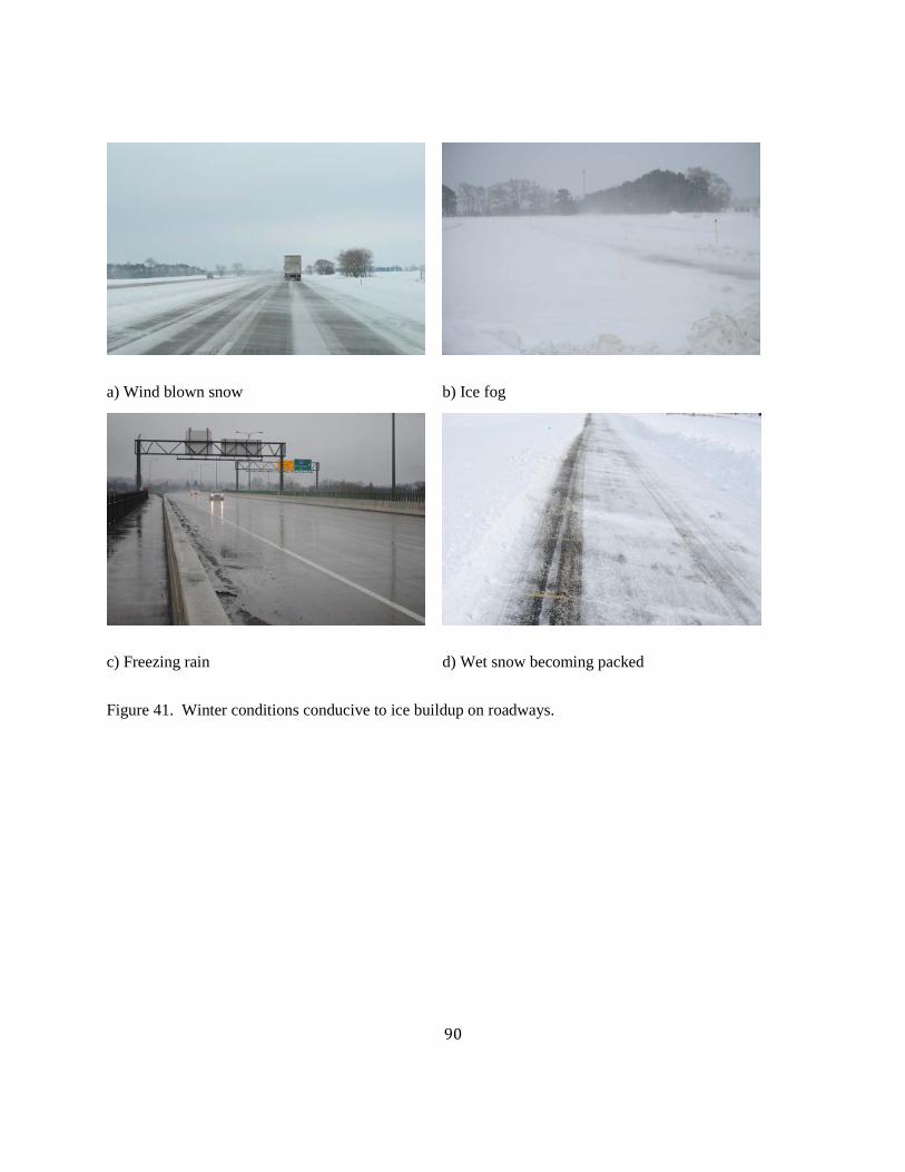
90
a) Wind blown snow b) Ice fog
c) Freezing rain d) Wet snow becoming packed
Figure 41. Winter conditions conducive to ice buildup on roadways.

91
a) MnDOT truck spreading solid deicer with prewet off left rear.
b) Brine application truck during demonstration (non-winter day).
Figure 42. Deicer and anti icer application equipment.

92
5.1: Test Method
5.1.1: Method design
For this evaluation of anti-icing persistence, measurements of flow and deicer concentration over time were made of storm drainage runoff from defined highway pavement areas. Unlike the field study previously described for this project (Task 1 Summary Report), this study was done in the laboratory to provide comparison between different pavement specimens in an attempt to identify factors related to pavement composition, construction, age and service.
Different deicer/anti icer chemicals were evaluated in response to application of artificial precipitation. Pavements were prepared by application of deicer chemical in either brine or solid form, dried or burnished, respectively, to replicate service conditions, then chilled. Measurements of chloride content were made to see how long the deicer chemical stuck to the pavement in relationship to the precipitation amount.
Initial exploratory evaluations used pavements chilled to 0, 15 and 28°F; however, this temperature regime created conditions unsuitable for testing as the artificial drainage froze to the pavement and become unaccountable for deicer content. For purposes of this evaluation, pavements were chilled to 40°F prior to precipitation application.
5.1.2: Pavement Samples
Pavement samples were obtained from Blue Earth County and the City of Mankato, rather than MnDOT, as by the time this research work had been authorized, excavated state highway pavements had been removed from maintenance and construction operations (pavements are typically ground or crushed in preparations for material reuse). Figure 43 shows student workers collecting a concrete pavement sample.
Collected pavement samples included:
• Limestone aggregate concrete pavement, approximately 60 years old, Blue Earth County State Aid Highway (CSAH) 17;
• Asphalt concrete pavement, approximately 1 year old (temporary pavement), CSAH 17; and,
• Asphalt concrete pavement, approximately 20 years old, Carney Avenue, Mankato, Minnesota.
Test sections of 8 inches by 8 inches (20 cm by 20 cm) were defined using weather stripping and silicone caulk to create hydraulic isolation on the pavement area of interest.
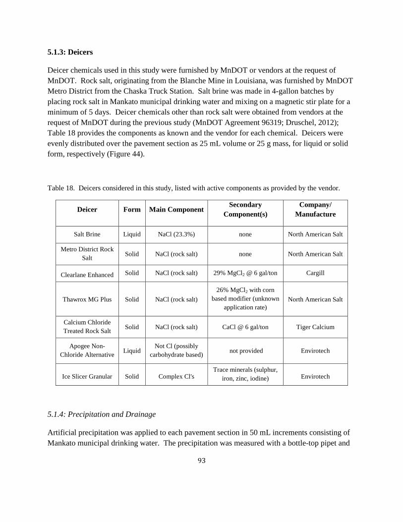
93
5.1.3: Deicers
Deicer chemicals used in this study were furnished by MnDOT or vendors at the request of MnDOT. Rock salt, originating from the Blanche Mine in Louisiana, was furnished by MnDOT Metro District from the Chaska Truck Station. Salt brine was made in 4-gallon batches by placing rock salt in Mankato municipal drinking water and mixing on a magnetic stir plate for a minimum of 5 days. Deicer chemicals other than rock salt were obtained from vendors at the request of MnDOT during the previous study (MnDOT Agreement 96319; Druschel, 2012); Table 18 provides the components as known and the vendor for each chemical. Deicers were evenly distributed over the pavement section as 25 mL volume or 25 g mass, for liquid or solid form, respectively (Figure 44).
Table 18. Deicers considered in this study, listed with active components as provided by the vendor.
Deicer Form Main Component Secondary
Component(s) Company/
Manufacture
Salt Brine Liquid NaCl (23.3%) none North American Salt
Metro District Rock Salt Solid NaCl (rock salt) none North American Salt
Clearlane Enhanced Solid NaCl (rock salt) 29% MgCl2 @ 6 gal/ton Cargill
Thawrox MG Plus Solid NaCl (rock salt) 26% MgCl2 with corn
based modifier (unknown application rate)
North American Salt
Calcium Chloride Treated Rock Salt Solid NaCl (rock salt) CaCl @ 6 gal/ton Tiger Calcium
Apogee Non-Chloride Alternative Liquid
Not Cl (possibly carbohydrate based) not provided Envirotech
Ice Slicer Granular Solid Complex Cl's Trace minerals (sulphur,
iron, zinc, iodine) Envirotech
5.1.4: Precipitation and Drainage
Artificial precipitation was applied to each pavement section in 50 mL increments consisting of Mankato municipal drinking water. The precipitation was measured with a bottle-top pipet and

94
gently released to the treated pavement (Figure 45a). Drainage was then collected from along the pavement test section perimeter using a transfer pipet (Figure 45b), measured and placed in a 60-mL centrifuge tube. Eight aliquots of precipitation were applied to each treated pavement specimen, and drainage collected after each application.
Drainage was evaluated for chloride content using a salinity refractometer with automatic temperature compensation (Model 211ATC, General Tools & Instruments, LLC, New York, New York) that measures salinity in a range of 0 – 10%.
Figure 43. Pavement specimen collection, CSAH 17 project

95
Figure 44. Anti icer application to defined pavement area.
Figure 45. Precipitation water application (left) and drainage collection (right).

96
5.2: Results
Numerical results and graphs are provided in Appendix A, broken out by each of the seven deicers tested. Each deicer was tested in triplicate for each pavement sample, both asphalt concrete and Portland cement concrete. The numerical results provide: application rate; precipitation volume and equivalent impingement depth (precipitation in inches); the volume recovered and the equivalent runoff depth; salinity measured in parts per thousand (ppt); and the cumulative salt equivalent in both total mass (grams) and mass per area calculated in pounds per lane mile. The graphs are of salinity and cumulative mass per area graphed by precipitation depth.
To evaluate variability between pavement specimens of each pavement composition, two asphalt concrete and two Portland cement concrete specimens were tested with salt brine. All other deicers were tested with a single pavement specimen. Results for asphalt concrete pavement are shown as circles and a dashed line for salinity and cumulative mass per area, respectively (squares and a dotted line for the second asphalt concrete specimen with salt brine). Results for Portland cement concrete pavement are shown as diamonds and a solid line for salinity and cumulative mass per area, respectively (triangles and a long dashed/dot line for the second Portland cement concrete specimen with salt brine).
All graphs were prepared using the same horizontal and vertical scales except for Apogee, which has a cumulative mass per area scale range that is twice the ranges of the other materials.
5.3: Evaluation
General trends were similar for all tests, as seen in the graphs provided in Appendix A. Salinity values start high at levels of 45 to 90 ppt at 0.10 inches or less precipitation, then declined to a low residual amount of less than 10 ppt by 0.30 inches precipitation. The decline in salinity values followed a highly similar curvature for all materials, likely reflecting solubility mechanics for surface films. The decline to residual amounts occurred between 0.1 and 0.3 inches precipitation consistently for all deicers.
Cumulative salt equivalent amounts initially increase quickly, and then settle above 0.30 inches precipitation into slow and steady increases with greater precipitation. Typical cumulative salt equivalent amounts are calculated at 2000 – 3000 pounds per lane mile, except for Apogee, which produced cumulative salt equivalent amounts of 4500 – 5500 pounds per lane mile, and salt brine, which produced cumulative salt equivalent amounts of 1000 – 3500 pounds per lane mile. Given the salinity residual behavior, the curve form associated with cumulative salt equivalent meets expectations.
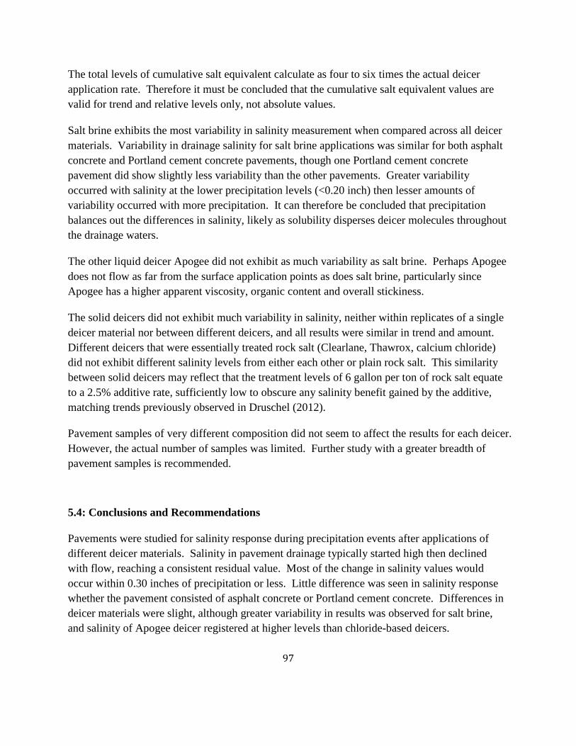
97
The total levels of cumulative salt equivalent calculate as four to six times the actual deicer application rate. Therefore it must be concluded that the cumulative salt equivalent values are valid for trend and relative levels only, not absolute values.
Salt brine exhibits the most variability in salinity measurement when compared across all deicer materials. Variability in drainage salinity for salt brine applications was similar for both asphalt concrete and Portland cement concrete pavements, though one Portland cement concrete pavement did show slightly less variability than the other pavements. Greater variability occurred with salinity at the lower precipitation levels (<0.20 inch) then lesser amounts of variability occurred with more precipitation. It can therefore be concluded that precipitation balances out the differences in salinity, likely as solubility disperses deicer molecules throughout the drainage waters.
The other liquid deicer Apogee did not exhibit as much variability as salt brine. Perhaps Apogee does not flow as far from the surface application points as does salt brine, particularly since Apogee has a higher apparent viscosity, organic content and overall stickiness.
The solid deicers did not exhibit much variability in salinity, neither within replicates of a single deicer material nor between different deicers, and all results were similar in trend and amount. Different deicers that were essentially treated rock salt (Clearlane, Thawrox, calcium chloride) did not exhibit different salinity levels from either each other or plain rock salt. This similarity between solid deicers may reflect that the treatment levels of 6 gallon per ton of rock salt equate to a 2.5% additive rate, sufficiently low to obscure any salinity benefit gained by the additive, matching trends previously observed in Druschel (2012).
Pavement samples of very different composition did not seem to affect the results for each deicer. However, the actual number of samples was limited. Further study with a greater breadth of pavement samples is recommended.
5.4: Conclusions and Recommendations
Pavements were studied for salinity response during precipitation events after applications of different deicer materials. Salinity in pavement drainage typically started high then declined with flow, reaching a consistent residual value. Most of the change in salinity values would occur within 0.30 inches of precipitation or less. Little difference was seen in salinity response whether the pavement consisted of asphalt concrete or Portland cement concrete. Differences in deicer materials were slight, although greater variability in results was observed for salt brine, and salinity of Apogee deicer registered at higher levels than chloride-based deicers.

98
It is recommended that more pavement samples be evaluated, with a particular focus on different pavements including open graded pavements and pavements of different ages. Brine mixtures should also be considered, as was done in a related study (Druschel, 2012), though issues of precipitation formation causing clogging would need to be considered concurrently.
99
Chapter 6: Conclusions
Three research approaches were used to study winter roadway maintenance. First, a deicer and anti-icer test facility was set up and procedures were established. Eight drainage locations of US 169 were routed through flow cells for measurements of chloride content and flow. Comparisons suggested good experimental behavior in the method, except for anomalous readings caused by instruments frozen in ice and effects caused by debris blockage. Efforts to protect and clean gear during deployment increased reliability. Of the measurements, it was observed that:
• temperature makes a good variable to check on instrument operating conditions; • conductivity and therefore chloride concentration were only affected by a lack of mixing
due to ice or sedimentation in the flow-through cells; and, • depth and therefore flow measurement were sensitive to ice buildup and debris blockage.
Chloride mass amounts passing through the drainage locations were calculated at levels substantially below the likely roadway application levels. This observation was consistent through the study area, regardless of traffic condition or direction. This finding agrees with observations by previous researchers that the majority of deicer loss occurs through traffic-induced spray or dust combined with plow “throw.” It is recommended that future efforts incorporate atmospheric sampling and off-roadway drainage measurement to assess chloride migration through such effects. Some evidence was observed of possible wind effects in the pathway of chloride on the roadways of the study site.
Results of two closely spaced storms suggested little to no persistence in chloride after a storm event. This result was intriguing, as it indicates that anti-icing could be detrimentally affected by any antecedent moisture prior to the anticipated icing event. Additional evaluation of this effect will occur during the upcoming Task 4 Pavement Study of this contract.
Second, a plowing and deicing test facility was set up and procedures were established. Six and three parallel 1,000-foot long lanes were created at two facilities offering a range of snow conditions. Time-lapse photography worked well to document plowing and melting conditions, at least during daylight hours. Ice base creation procedures were developed but remain somewhat difficult to do in winter conditions without a ready supply of cold water.
Similar plowing results were obtained across six different lanes at one facility, suggesting strong replication of performance. Results appeared consistent over the length of the lanes, based on the photographs. Similar results were also seen when plowing was compared between two sites with slightly different snow conditions, suggesting uniformity in results from a single truck, plow and driver combination. Plowing results followed expectations for differences in speed, in

100
that snow rises higher in the curvature of the plow in response to higher speeds, and higher speeds create a broader spray off the plow ends, with an accompanying greater distribution distance of the dislodged snow.
Deicing results followed the expectations developed in laboratory studies for temperature, with warmer temperatures providing more melt from the deicer. Little melt was observed below about 10° F unless sunlight provided warming. Additional work is needed to evaluate deicing behaviors when faced with changing temperatures, i.e., formation of refreeze when temperatures drop but the roadway is still wet with brine, activation of deicing when temperatures rise from a cold application temperature, etc. Time of the melting process did not appreciably change with temperature, and any changes noted may be more related to the increased ice melt capacity with increased temperature. However, additional work could be done to fine tune the melt time characteristics, perhaps with closer photography at more rapid increments.
No significant difference was observed in deicer performance by whether prewet was used or not. Benefits reported by maintenance personnel of better roadway adherence during windy conditions and quicker initiation of melt were not observed during this study, and could warrant further evaluation if deemed important. Traffic, specifically truck traffic, was found to cause a significant improvement in deicer performance, with both wider and quicker melt occurring. The interaction of tire pressure and deicer was clearly observed to create the improved melting, as compared to the effect of the tire pressure alone.
Third, pavements were studied for salinity response during precipitation events after applications of different deicer materials. Salinity in pavement drainage typically started high then declined with flow, reaching a consistent residual value. Most of the change in salinity values would occur within 0.30 inches of precipitation or less. Little difference was seen in salinity response whether the pavement consisted of asphalt concrete or Portland cement concrete. Differences in deicer materials were slight, although greater variability in results was observed for salt brine, and salinity of Apogee deicer registered at higher levels than chloride-based deicers.

101
References
Blackburn, Robert R., Erin J. McGrane, Cecile C. Chappelow, Douglas W. Harwood, and Edward J. Fleege. 1994. Development of anti-icing technology. Washington, DC: Strategic Highway Research Program, National Research Council, SHRP-H-385.
Blackburn, Robert R., Erin J. McGrane, Karin M. Bauer, and Edward J. Fleege. 1993. “Current status of U.S. anti-icing technology” Transportation Research Board Record No. 1387, pages 29-39. Symposium on Snow removal and ice control technology. Washington, D.C.: National Academy Press.
Blomqvist, G., M. Gustafsson, M. Eram, and K. Unver. 2011. “Prediction of salt on road surface tool to minimize use of salt.” Transportation Research Record, (2258), 131-138.
Bolen, W. P. 2014. Salt Commodity Summary. Downloaded June 7, 2014 from http://minerals.er.usgs.gov/minerals/pubs/commodity/salt/mcs-2014-salt.pdf. United States Geological Survey, Washington, D.C.
Chollar, B. H. 1988. “Field evaluation of calcium magnesium acetate during the winter of 1986-87.” Public Roads 52 (1) (June 1988): 13-18.
Druschel, S.J. 2012. Salt Brine Blending to Optimize Deicing and Anti-Icing Performance, Minnesota Department of Transportation, St. Paul, MN.
Committee on the Comparative Costs of Rock Salt and Calcium Magnesium Acetate (CMA) for Highway Deicing. 1991. Highway deicing comparing salt and calcium magnesium acetate. Transportation Research Board, Special Report 235. Washington, D.C.: National Academy Press.
Highway Innovative Technology Evaluation Center (HITEC). 1999. Summary of evaluation findings for the testing of ice ban. Washington DC: Civil Engineering Research Foundation.
Ketcham, Stephen A., L. David Minsk, and Lawrence S. Danyluk. 1998. Test and evalutation project no. 28 : Anti-icing technology, field evaluation report. Springfield, VA: Federal Highway Administration.
Manning, David G., and Max S. Perchanok. 1993. “Trials of calcium magnesium acetate deicer on highways in Ontario,” Transportation Research Board Record No. 1387, pages 71-78.

102
Symposium on snow removal and ice control technology. Washington, D.C.: National Academy Press.
Raukola, Tapio, Rauno Kuusela, Heikki Lappalainen, and Antti Piirainen. 1993. “New ideas and equipment for winter maintenance in Finland,” Transportation Research Board Record No. 1387, pages 48-56. Symposium on Snow removal and ice control technology. Washington, D.C.: National Academy Press.
Shi, Xianming, Keith Fortune, Robert Smithlin, Michelle Akin, and Laura Fay. 2013. “Exploring the performance and corrosivity of chloride deicer solutions: Laboratory investigation and quantitative modeling.” Cold Regions Science and Technology 86 (0) (2): 36-44.
Stotterud, Roar, and Knut Magne Reitan. 1993. “Deicing of roads in Norway with brine” Transportation Research Board Record No. 1387, pages 23-28. Symposium on Snow removal and ice control technology. Washington, D.C.: National Academy Press.
Sypher:Mueller. 1988. 1987-1988 City of Ottawa de-icer field trials. Ottawa, Ontario, Canada: City of Ottawa Department of Engineering and Works.
Trost, Susan E., Frank J. Heng, and E. L. Cussler. 1987. “Chemistry of deicing roads: Breaking the bond between ice and road.” Abstract. Journal of Tranportation Engineering 113, no. 1:15-26.
Woodham, D. 1994. Alternative deicing chemicals research. Denver, Colorado: Colorado Department of Transportation.