NCAA TR ERL J59-GL£RL

*T

NOAA Technical Report ERL LERL 8U.S. DEPARTMENT OF COMMERCENATIONAL OCEANIC AND ATMOSPHERIC A D M i W S T R A T ONEnvironmental Research Laboratories

Saginaw Bay Water Circulation

J. H. SAYLOR

3OULDER. COLO.DECEMBER 1975

^WMOSfl^ U.S. DEPARTMENT OF COMMERCE

Rogers C. B. Morton, Secretary

NATIONAL OCEANIC AND ATMOSPHERIC ADMINISTRATION

Robert M. White, Administrator

ENVIRONMENTAL RESEARCH LABORATORIES

Wilmot N. Hess, Director

NOAA TECHNICAL REPORT ERL 359-GLERL 6(GLERL Contribution No. 45)

Saginaw Bay Water Circulation

L. J. DANEK

J. H. SAYLOR

BOULDER, COLO-December 1975

FOREWORD

This report presents the results of a field study conductedduring the summer of 1974 on Saginaw Bay, Michigan. Both Lagrangianand Eulerian current measuring techniques were used to determinethe characteristic water circulation patterns of the bay and tofind representative current speeds and volume transports duringthe summer. This study was partially supported through an inter-agency agreement with the National Environmental Research Center,Office of Research and Development, Environmental ProtectionAgency, under contract EPA-IAG-D4-0502 and is a contribution tothe International Joint Commission Upper Lakes Reference study.

11

NOTICE

The NOAA Environmental Research Laboratories do notapprove, recommend, or endorse any proprietary product orproprietary material mentioned in this publication. Noreference shall be made to the NOAA Environmental ResearchLaboratories, or to this publication furnished by the NOAAEnvironmental Research Laboratories, in any advertising orsales promotion which would indicate or imply that the NOAAEnvironmental Research Laboratories approve, recommend, orendorse any proprietary product or proprietary materialmentioned herein, or which has as its purpose an intent tocause directly or indirectly the advertised product to beused or purchased because of this NOAA Environmental ResearchLaboratories publication.

CONTENTS

Page

ABSTRACT 11. INTRODUCTION 12. PREVIOUS STUDIES 33. METHODS OF DATA COLLECTION 4

3.1 Current Meters " " 43.2 Drogues 53.3 Wind 6

4. RESULTS 64.1 Drogues 64.2 Current Meters , 124.3 Power Spectra 17

5. CONCLUDING REMARKS 196. REFERENCES 217. APPENDIX A. DROGUE RESULTS 228. APPENDIX B- MONTHLY CURRENT DIRECTION HISTOGRAMS 369. APPENDIX C. POWER SPECTRA ESTIMATES 43

FIGURES

1. The study site showing the locations of the 9 current metermoorings and the wind station at Gravelly Shoal Lighthouse. 2

2. Compilation of drogue tracks for a southwest wind from6 June, 8 June, 14 June, 21 August, and 22 August. 7

3. Circulation pattern for a southwest wind. 84. Compilation of drogue tracks for a northeast wind from

23 August, 28 August, and 12 October plus average velocityvector from meter 9A. 9

5. Circulation pattern for a northeast wind. 106. Histograms of current direction for entire period of study. 137. Histograms from 22-27 June — northeast wind. 148. Histograms from 20-22 July — northeast wind. 159. Histograms from 20-22 August — southwest wind. 1610. Histograms from 3-5 October — southwest wind. 1711. Progressive vector plot of data from current meter 2B

showing 17.1-hr inertial period. 18

TABLE

1. Current meter locations and dates of operation.

APPENDIX A FIGURES

A.I.A. 2.A. 3.A. 4.A.5.A. 6.A. 7.A. 8.A.9.A. 10.A. 11.A. 12.A. 13.

DrogueDrogueDrogueDrogueDrogueDrogueDrogueDrogueDrogueDrogueDrogueDrogueDrogue

resultsresultsresultsresultsresultsresultsresultsresultsresultsresultsresultsresultsresults

fromfromfromfromfromfromfromfromfromfromfromfromfrom

6 June and 7 June.8 June and 10 June.12 June and 13 June.14 June and 15 June.20 August and 21 August.22 August and 23 August.24 August and 26 August.28 August and 29 August.30 August and 2 October.3 October and 7 October.8 October and 9 October.10 October and 11 October12 October.

Page

23242526272829303132333435

APPENDIX B FIGURES

B.I.B.2.B.3.B.4.B.5.B.6.

HistogramsHistogramsHistogramsHistogramsHistogramsHistograms

of currentof currentof currentof currentof currentof current

direction for May.direction for June,direction for July.direction for August,direction for September,direction for October.

373839404142

APPENDIX C FIGURES

C.I. Power spectra2A and 2B.

C.2. Power spectra4A and 4B.

C.3. Power spectra5A and 5B.

C.4. Power spectra3B and 6B.

C.5. Power spectraC.6. Power spectra

2A and 5B.C.7. Power spectra

6B and 9A.

estimates for data from current meters

estimates for data from current meters

estimates for data from current meters

estimates for data from current meters

estimate for data from current meter 9A,estimates for data from current meters

estimates for data from current meters

vi

44

45

46

4748

49

50

SAGINAW BAY WATER CIRCULATION

L. J. Danek and J. H. Saylor

A combination of Lagrangian measurements and fixed currentmeter moorings during the summer of 1974 were used to determinethe circulation patterns of Saginaw Bay. Because the bay isshallow, the water responds rapidly to wind changes. Distinctcirculation patterns were determined for a southwest wind and anortheast wind._.. Speeds measured in the inner bay are on theorder of 7 cm s wnereas n the outer bay the speeds averagecloser to 11 cm s . A.typical exchange rate between the innerand outer bay is 3700 m s for winds parallel to the axis ofthe bay, but winds perpendicular to the axis of the bay causelittle water to be exchanged.

The driving forces that control the circulation patternsin the bay are also examined. The water motions in the innerbay are driven almost solely by wind stress whereas the outerbay is also influenced by the circulation of Lake Huron andby the geometry of the area. Inertial oscillations are themost dominant periodic component of the flow. Seiche motions ofLake Huron and the bay itself were detected, but they are of lit-tle importance in determining the gross circulation of the bay.

1. INTRODUCTION

This report presents results of a 1974 field investigation of SaginawBay water currents and circulation patterns. Saginaw Bay is located on thesouthwestern coast of Lake Huron, centered at nearly 44°00'N latitude and83°20'W longitude, as shown in fig. 1. The investigative program includedthe deployment of nine current meter moorings in the bay (fig. 1) inMay, 1974, the establishment of a wind recording station at the GravellyShoal Lighthouse, and Lagrangian current measurements by use of drogues dur-ing three 2 week-long intervals while the moored current meters were inplace. The current meters were retrieved in October 1974, giving approxi-mately 5 months of continuous current speed and direction recordings.

The mouth of Saginaw Bay (from Point Aux Barques to Au Sable Point)is 42 km wide and has an average depth of 27 m. The bay's narrowest con-striction is between Sand Point and Point Lookout with a width of 20 kmand a mean depth of only 4m. A line between these two points forms anapproximate boundary between the outer bay (mean depth 16 m) and the muchshallower inner bay (mean depth 4.5 m). The bay is 83 km long with itsmajor axis aligned 40° east of north. An important feature of the bay isthe relatively deep channel that runs through the inner bay. It is alignednearly parallel with the major axis of the bay and has a maximum depth ofabout 14 m. The Saginaw River, which enters the bay at the southwestern

2end, drains an area of over 16,000 km and passes through Bay City justprior to entering the bay. The average discharge of thj river is about100 m s , though it can increase to well over 300 m s during the springmonths. There are several small rivers that also flow into the bay, buttheir combined discharge is small compared to that of the Saginaw River.

S agin aw BayMichigan

N

Au Sable Point]

Figure 1. The study site showing the locations of the 9current meter moorings and the wind station at GravellyShoal Lighthouse.

Because the water in the inner reaches of Saginaw Bay is shallow,currents in the inner bay are closely related to the wind; the measure-ments presented in this report establish the wind dependence. The outerbay interacts strongly with the larger scale circulation of Lake Huron.Saginaw Bay currents and the character of Saginaw Bay-Lake Huron inter-

actions are important because of the heavy load of pollutants which enterLake Huron through the bay. The Saginaw River discharges the wastes ofthe industrialized cities of Midland, Bay City, and Saginaw, Mich., and isthe largest tributary source of undesirable materials discharged to LakeHuron. A long residence time and the pattern of water mass movement withinSaginaw Bay have adversely impacted parts of the bay.

2. PREVIOUS STUDIES

Several qualitative studies have been done on the circulation of LakeHuron and Saginaw Bay. The first was by Harrington (1895), who conducteda drift bottle study on Lake Huron during 1892, 1893, and 1894. He con-cluded that the currents were quite variable, but that there was usuallya strong southward current along the west shore of the lake. This currenteither passed by or flushed through the mouth of Saginaw Bay, in eithercase strongly influencing the circulation in the outer bay.

Ayers et al. (1956) used c. dynamic height method for fresh water plusverification from a drift bottle study to determine the circulation ofLake Huron. It was concluded that the usual summertime circulation wascounterclockwise with strong southward flow along the west shore of LakeHuron. Part of this southward flow entered the northern part of the mouthof Saginaw Bay, flushed through the outer bay, and flowed eastward to LakeHuron along the southern coast. The flow then continued southward alongthe west coast of Lake Huron. They also suggested that a similar counter-clockwise loop existed in the inner bay, with water entering the bay alongthe west shore and flowing out along the east shore, and that at timesa slowly rotating eddy occurred near the mouth of the outer bay.

Johnson (1958) performed extensive drift bottle studies in SaginawBay and Lake Huron. His findings confirmed the earlier observations of astrong southerly current along the western shore of Lake Huron, and hemade special note of the prominence of this current in the southern partof Lake Huron below the mouth of Saginaw Bay. In the bay itself, he con-cluded that normally a counterclockwise gyre exists, with water enteringthe bay along the west shore and leaving along the east shore in a fashionsimilar to that suggested by Ayers et al. He states, however, that it isdifficult to generalize about the circulation of the bay because it is sohighly dependent on local winds, adding that ".... it seems possible thata surface current might change in response to a rapidly changed strongwind in a matter of hours," (Johnson, 1958, p. 16).

— 4-Beeton et al. (1967) used chemical distributions, mainly Cl and Na ,

to trace the water movements in the bay. They determined that winds fromthe northeast, east, and southeast produce a clockwise circulation inSaginaw Bay and west and southwest winds drive a counterclockwise circula-tion. They state that the circulation can shift from clockwise to counter-clockwise in a matter of 4 days or less, a conclusion also suggested bydata from the Michigan Stream Control Commission (1937). Beeton et al.also stated that the flow of Saginaw River water was out of the bay along

the eastern shore and that this deflection to the right may be influencedby the Coriolis force. Rogers et al. (1975) used remote sensing to detectwater masses in Saginaw Bay. They used Earth Resources Technology Satte-lite (ERTS) imagery plus ground truth data collected by the EnvironmentalProtection Agency (EPA) to map areas of constant turbidity. Their workshowed that during the 1 day of investigation, more turbid water wasfound along the eastern shore. This again suggested that clearer LakeHuron water entered Saginaw Bay along the west shore, mixed with more tur-bid Saginaw River water, and exited along the eastern shore of the bay.

Allender (1975) developed a numerical model to simulate the circu-lation of Saginaw Bay. The development of such a model requires the speci-fication of boundary conditions at the mouth of Saginaw Bay with LakeHuron. By examining water level records from within Saginaw Bay and fromLake Huron near the bay mouth, Allender concluded that prominent bay modesof 3.3 hr and 1.8 hr were driven by forcing waves with these periods inLake Huron; shorter period waves were felt to be strongly damped in thebay. Therefore, periodic functions of the velocity field were specifiedas boundary conditions at the bay mouth, adjusted in intensity to yieldSaginaw Bay water surface oscillations near the observed amplitudes. Hestated that the circulation pattern of the bay can change completely in8 hr or less, fully responding to a newly-imposed wind stress and reachinga new equilibrium state. The general pattern derived in the inner bay wascurrent flow in the same direction as the wind in shoal areas with returnflow in the deeper channel near the center of the bay. Since the prevail-ing wind is from the southwest, the usual circulation was characterizedby water from the outer bay entering through the deep channel and leavingalong the eastern coast.

A recent study of Lake Huron currents by Sloss and Saylor (1975)examined current meter records from Lake Huron and the mouth of SaginawBay. They noted the strong southward current along the west shore of LakeHuron north of Saginaw Bay, but did not speculate on circulation patternsin the bay itself. A detailed review of chemical, biological, and physicalstudies of Saginaw Bay and a discussion of the hydrology of the area ispresented in Freedman (1974).

3. METHODS OF DATA COLLECTION

3.1 Current Meters

Eighteen Geodyne model A-100 film recording current meters wereinstalled in Saginaw Bay during May, 1974, and were operational throughOctober, 1974. A maximum of three current meters were attached to ananchored line and suspended in the water column by a subsurface float. Asmall surface float attached to the end of a ground line 30 to 40 m inlength was used to mark the location of the moorings and to aid in therecovery of the meters. Because of mechanical and electrical problems,several of the meters failed; this left some holes in our proposed samplinggrid. Locations and depths of the meters are given in fig. 1 and table 1.

Table 1. Current Meter Locations and Dates of Operation,

Meter No,

9A

Site No, Lat. (N) Long. (W) Depth (m) Duration

2A2B2C

3B3C

4A4B

5A5B

6A6B

222

33

44

55

66

44°5.2'44°5.2'44°5.2'

44°11.5?44°11.5'

44°15.3'44°15.3'

44°10.1'44°10.1'

44°2.3'44°2.3'

83°2.4'83°2.4f83°2.4'

83°10.9'83"10.9?

83°15.0'83°15.0'

83°28.9'83°28.9'

83°17.3'83°17.3'

102030

2030

1020

715

710

17 May-15 Oct.28 May-15 Oct.17 May-15 Oct.

18 May-15 Oct.18 May-15 Oct.

18 May-15 Oct.18 May-15 Oct.

18 May-16 Aug.18 May-3 Oct.

17 May-8 June17 May-16 Oct.

43°45.6! 83°41.4' 20 May-18 Oct

Each current meter sampled the velocity for a 50-s interval every30 min and accumulated over 7200 data points for the duration of the_study.The Savonius rotors on the meters have a threshold speed of 2.5 cm s andan accuracy of 2.5 cm s for speeds less than 50 cm s . The sensitivityof the direction vane is alignment within 10° of the current direction ata current speed of 2.5 cm s , and within 2° at 10 cm s , with a resolu-tion of 2.8°. The meters recorded the velocity in binary code on standard16-mra photographic film. Eight of the films were sent to Geodyne for auto-mated processing and the decoded raw data was stored on magnetic tape.The rest of the films were read and decoded manually.

3.2 Drogues

Drogues were tracked for three 2-week sessions from abroad the R/VShenehon, one session each in June, August, and October of 1974. Theresults are shown in Appendix A. The drogues consisted of a surface buoyplus a subsurface panel. The buoy was made from a pneumatic float and aradar reflector that extended 1.5 m above the water surface. The panel wasa current cross made of sheet metal that could be set to any desired depthin the water column. During this study the panels were set only.at depthsof 2 m or 5 m. The cross-sectional area of the panel was 1.86 m . One

drogue and one anchored radar reflector were deployed at each launch site,and the drogues were tracked by radar using the anchored buoy as a refer-ence point. Typically five drogues were launched along each transect witha 2.5-kra spacing between drogues.

3.3 Wind

A wind station was installed at the Gravelly Shoal Lighthouse nearPoint Lookout. Both wind speed and direction were measured by a Bendixwind recording system. The data was continuously recorded on a stripchart and later digitized into hourly averages. The sensor location wasapproximately 23 m above the water surface. The distance to the nearestpoint of land was 4.5 km, so that local interferences were minimal. Dueto the isolated location of the station, constant servicing was not pos-sible. Consequently a few relatively short gaps appeared in the data.The gaps included about 10 days of record during the 5-month study. Forcomputation of monthly wind statistics, the gaps were filled with dataobtained from Tri-City Airport (located 20 km WSW of Bay City) after windspeeds were adjusted to make them more consistent with the generally higherspeeds measured at the lighthouse. The adjustment procedure followed wasto average the speeds recorded for 1 week prior and 1 week after the gap inthe record at both the lighthouse and the airport and adjust the airportspeed during the record gap by the observed ratio of speed difference.

4. RESULTS

4.1 Drogues

Since most of the inner bay was too shallow for current meter moor-ings, the drogue studies were concentrated in this area. The results areplotted on figs. A. 1 through A. 13. During 25 days on the bay, 117drogues were tracked for an average of 5 hr each. The average speed forthe drogues was 6.7 cm s . The speeds in several areas of the bay variedconsiderably from this average. Near Point Lookout, where., the channel hasits narrowest constriction, the average speed was 10 cm s . The waterentering or leaving the bay was apparently funneled through this constric-tion, causing the higher speeds. The water in the southeastern sectionof the bay was nearly stagnant, with average speeds less than 4 cm sThis is the same area where the highest ion concentrations were reportedby Beeton, et al. (1967). In the central part of the inner bay the speedswere typically slower in the channel (average speed 6.2 cm s ^ than inthe shallow water areas on either side (average speed 8.8 cm s ).

All of the drogue panels were set at a depth of either 2 m or 5 m.There was no appreciable difference between the average speeds measuredat the two levels. One exception to this was on 6 June (fig. A. 1), whenthe speed measured at the 2-m level was more than twice the speed at the5-m depth. There was also a difference in direction between the two levelsof approximately 30°. The reason for the difference was bottom friction,as the water was only 7-m deep and the 5-m drogue was deep enough to be

in the region where the bottom effects were important,were drogue panels set that close to the bottom.

Only on that day

Since it was not possible to do a synoptic survey of the entire bay,the drogue data were compiled to present on one chart observations madeduring similar wind conditions in various parts of the bay. This provideda reasonably accurate picture of the circulation of the inner bay for twoprevailing wind directions. The transects from 6 June, 8 June, 14 June,21 August, and 22 August are plotted on fig. 2. The wind was out of thesouthwest during all of these days. The results show that the circulation

Figure 2. Compilation of drogue tracks for a southwestwind from 6 June, 8 June, 14 June,, 21 August, and22 August.

is characterized by a clockwise gyre in the western portion of the innerbay (fig. 3). The water in the shallow eastern area flows in the samedirection as the wind and enters the outer bay between Charity Island andOak Point. There is a well defined return flow in the channel past PointLookout which fans out somewhat as it enters the inner bay. The SaginawRiver water enters from the southwest and mixes with the bay water. Someof the river water then branches off into the western portion of the bay,but most of it flows into the shallow eastern area, causing the high ionconcentrations reported by Beeton et. al. (1967).

N

Figure 3, Ciroulati,on pattern for a southwest wi/nd.

The wind was usually out of the southwest, but there were a fewoccasions of northeast winds during the Lagrangian current studies. Thedrogue tracks for these days, 23 August, 28 August, and 12 October, areplotted on fig. 4. An average velocity was also computed from meter 9Afor these 3 days and the result plotted on the same figure. From this data

N

S IDcm/sac

Figure 4. Compilation of drogue tracks for a northeast windfrom 23 August, 28 August^ and 12 October plus averagevelocity vector from meter 9A.

the circulation driven by a northeast wind was determined and plotted onfig. 5. The flow is characterize^ by a counterclockwise gyre in thewestern inner bay. The water enters along the eastern shore betweenCharity Island and Oak Point and flows out in the channel past PointLookout. The circulation pattern is similar to that for a southwest windexcept that the current directions are just reversed.

N

Figure 5. Circulation pattern for a northeast wind.

10

On 22 August (fig. A. 6) the drogues were deployed across the channelnear PointLookout. The wind was out of the southwest with an average speedof 5.8 m s . Drogue panels were set at both 2 m and 5 m, making it possibleto estimate the vertical profile of horizontal velocity and to compute thevolume of water entering the inner bay. The estimated transport was3700* m s or 37 times the average flowqof,,the Saginaw River. Since thevolume of the inner bay is about 8.5 x 10 m , it would take only 26 1/2days for this flow to fill the inner bay.

It was also possible to estimate the volume of return flow in thechannel from the drogue tracks of 14 June (fig. A. 4). The wind was againout of the southwest with an average speed of 5.0 m s . The estimatedreturn transport was 7100 m s . This is larger than the previous esti-mate, but this transect was further south and much of the transport wasdue to the recycling of water from the shallow western region as illustratedin fig. 3.

The highest speeds were recorded during a storm on 26 August (fig. A.7), with wind again out of the southwest. The drogues were deployed in thechannel and were in the region of ..the return flow, therefore moving intothe wind. Speeds of over 30 cm s were measured, which represents a re-turn transport of 18,600 m s through this section of the channel. Thespeeds and transports measured may have been even higher because the droguemovements were no doubt somewhat impeded by the strong wind.

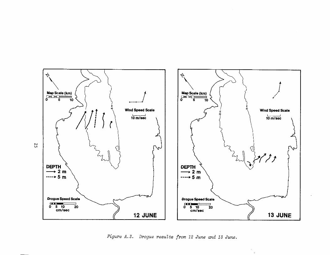
On several days the wind changed rather abruptly and became steadyout of the southwest. This presented an opportunity to examine the responseof the bay to sudden wind changes. The typical response is that in allareas of the inner bay the water initially moves with the wind. Afterapproximately 8 hr a return flow developes in the central channel of thebay. Of course residual currents and the intensity of the wind affect thecirculation and lag time before a return flow developes and a new equili-brium state is established, but the above results seem typical for a south-west wind. On 12 June (fig. A. 3) and 8 October (fig. A. 11) the water inthe shallow western section of the inner bay reacted to the wind changeby moving in the same direction as the wind. The easternmost drogue on12 June, though, had a much smaller velocity than the others. It waslaunched in the channel and its progress was retarded by the development ofthe return flow. On 29 August (fig. A. 8) the magnitude of the wind wassmall, but the development of the return flow could be seen along theeastern edge of the channel. On 20 August (fig. A. 5) the flow couldactually be seen reversing directions. The wind became southwesterly about0200. The current initially followed the wind, but between 1000 and 1100the flow reversed directions. Thus it took 8 to 9 hr for the return flow

* Transports and volumes referred to in this section have been calculatedusing the 1-m stage existing during the period of investigation. Physicaldimensions referred to in the introductory section were scaled from lakecharts giving depths relative to the International Great Lakes Datum (1955)

11

to develop. The magnitude of the bay wind was rather weak, however, and astronger wind would have caused the bay to fully respond more rapidly. Stillthis estimate agrees well with some of the previous work on the bay (Johnson,1958; and Allender, 1975).

Conductivity and chloride were measured at 5-min intervals enroute toand from the drogue transects during most of the Lagrangian current studies.The data collected, however, were not sufficient to trace the water massesin the bay. Because of the rapidly changing circulation patterns in thebay, samples taken on one day could not be correlated with previous days'measurements. In order to determine flow patterns with chemical analyses,a survey of the entire bay must be completed in a single day unless thestudy can be conducted during a period of relatively constant wind. Thedata collected, however, show a sharp gradient with values highest near theSaginaw River. The conductivity is twice as high near the mouth of theriver as the overall average of the bay. The values in specific areas ofthe bay varied considerably from day to day, but no general trends wereapparent.

4.2 Current Meters

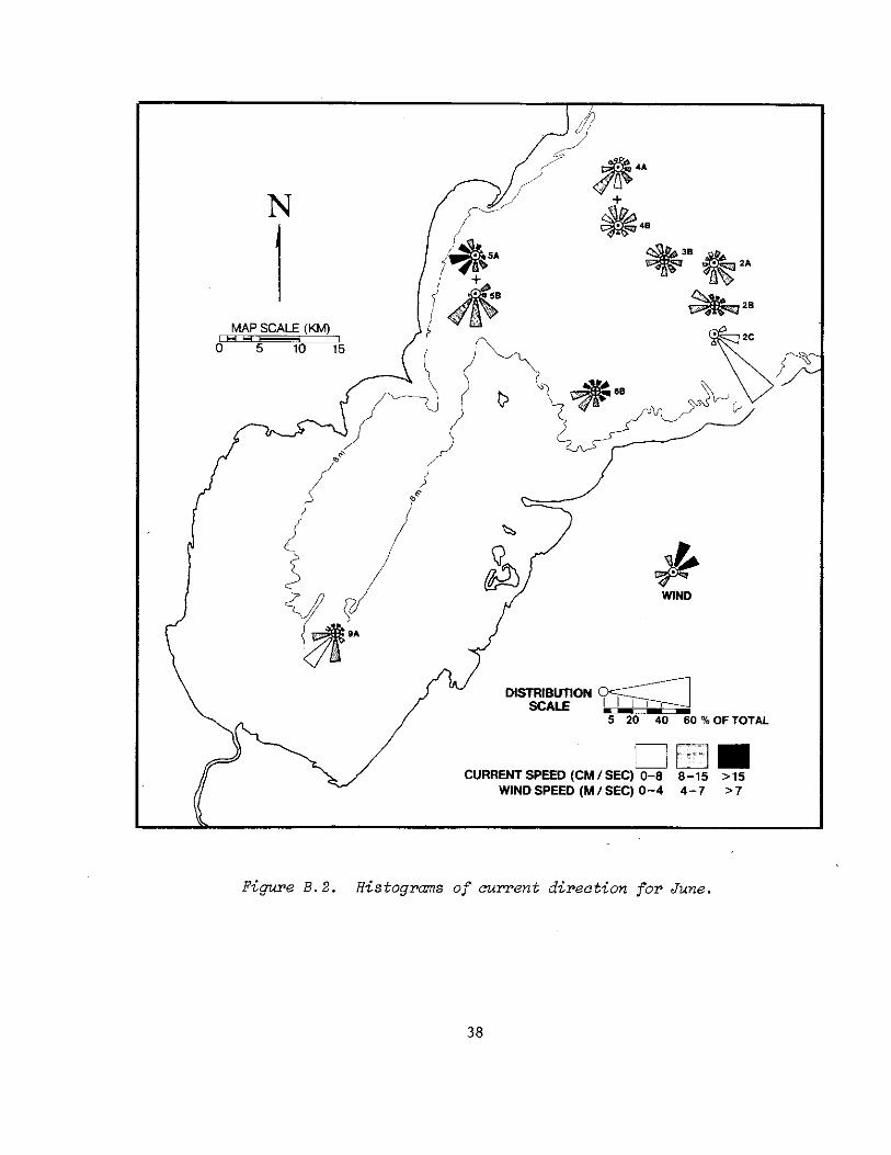
Since most of the inner bay was too shallow for current meter moorings,most of the meters were deployed in the outer bay (see fig. 1). Histogramsof current direction are used to display the data. The histograms wereconstructed by sorting the current direction into 40° sectors. The per-centage of data points falling into each sector was computed and the averagespeed for each sector was calculated. The average speeds.were divided intothree categories: low (<8 cm s ), medium (8 to 15 cm s ), and high(>15 cm s ), and the results are displayed on the histograms. Monthly his-tograms were computed for all of the meters and are shown in Appendix B.A similar summary of wind data for each month is given on the same figures.Histograms of current direction for the entire recording interval were alsocomputed and are shown in fig. 6.

The average speed computed for all the current meter data was10.6 cm s . The highest averages were recorded by meter 6B (13.7 cm s )and meter 5A (13.0 cm s ). These two meters were located near the divisionbetween the inner and outer bays. The-only meter in the inner bay (meter 9A)recorded an average speed of 7.9 cm s . The speed recorded at the 30-mlevel near the mouth of Saginaw Bay averaged only 7.7 cm s (meters 2Cand 3C). The direction* measured at the 30-m level was much more stable thanthe direction recorded closer to the water surface. This indicates thatthe flow along the bottom near the mouth is rather slow and relatively free,,of turbulence. Meter 6B, on the other hand, is located in an area of highturbulence. Large fluctuations in direction and a high variance calculatedfor the velocity components plus large amounts of energy in the high fre-quency range of computed power spectra (discussed in the next section) indi-cate that this is an area of strong turbulence. This meter is located nearthe division of the inner and outer bay. Apparently the water from the innerregion mixes with the water in the outer bay in this area and causes thesehighly variable currents.

12

N

5 20 40 SO % OF TOTAL

_CURRENT SPEED (CM /SEC) 0-8 8-15 >15

WIND SPEED (M / SEC) 0-4 4-7 > 7

Figure 6. Histograms of current direction for the entireperiod of study.

Histograms computed for the entire length of the current meter records(fig. 6) show the high variability of the flow, with the current directionfor some of the meters almost equally distributed around the compass. Thisis due not only to the variable winds, but also to the importance of iner-tial currents in certain parts of the bay. Meter 9A, though, shows a veryconsistent flow to the southwest. The prevailing wind is out of the south-west, causing a return flow to move down the channel past meter 9A andproducing the prominent flow in this area. Meter 5B shows a strong south-west flow near the mouth of the channel because it is in the zone of returnflow for southwest wind and in the inflow to Saginaw Bay from Lake Huronduring northeast wind.

13

N

CURRENT SPEED (CM/SEC) 0-8 8-15 >15

Figure 7. Histograms from 22-27 June — northeast wind.

Since the currents are so highly dependent on the local winds, the char-acter of the bay circulation during several meteorological events was exam-ined. Histograms of current direction were computed for periods when thewind was relatively constant for at least 2 days. Since the two predominantwind directions during the summer of 1974 were out of the southwest and out ofthe northeast, the response of the bay to winds from these directions wasanalyzed. On 22-27 June and 20-22 July the wind was constant out of thenortheast. The histograms for these periods were plotted on fig. 7 and 8,respectively.

CURRENT SPEED (CM /SEC) 0-8 8-15 >1S

Figure 8. Histograms from 20-22 July — northeast wind.

The results for the two episodes are quite similar. The flow in the outerbay is characterized by a counterclockwise gyre; water enters the bay at thenorthern edge of the mouth, flushes through the outer bay, and flows backinto Lake Huron along the southern part of the bay mouth as indicatedby the histograms at site 2. An illustration of this pattern, plus thecirculation derived from the drogue results for a northeast wind in theinner bay, is shown in fig. 5. The vectors on this illustration represent avertically averaged horizontal velocity.

15

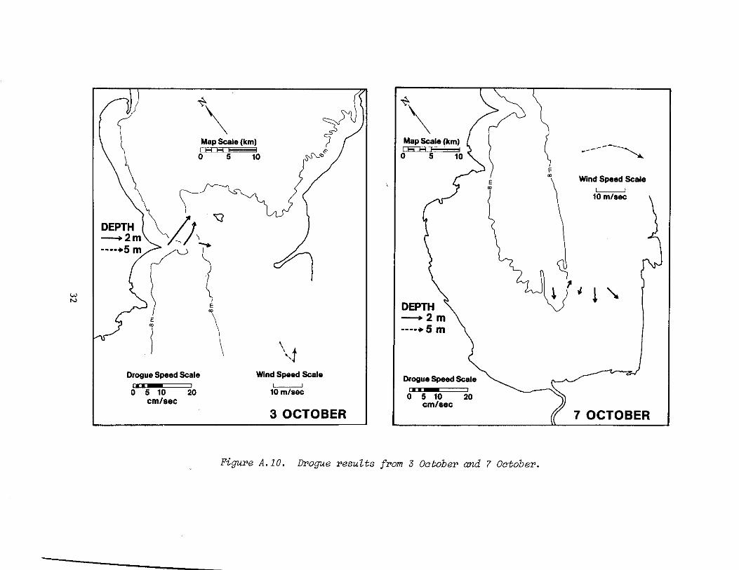
On 20-22 August and 3-5 October the wind was constant out of thesouthwest. The histograms for these periods are plotted on fig. 9 and 10.The results from these episodes are markedly different from those computedfor a northeast wind. The flow from Lake Huron enters the bay through thesouthern part of the mouth. The water flushes through the outer bay in aclockwise sense and flows out along the northern edge. This circulationpattern, plus the flow pattern determined from the drogue results for asouthwest wind, is illustrated in fig. 3. As noted earlier, the flow pastsite 5 is usually to the southwest under both wind conditions, influencedmore by the gross circulation and geometry of the bay than by the direct

influence of the local winds.

CURRENT SPEED (CM/SEC) 0-8 8-15 >15

Figure 9. Histograms from 20-22 August — southwest wind.

16

N

DISTRIBUTIONSCAL£ U Lai

5 20 40 60% OF TOTAL

CURRENT SPEED (CM/SEC) 0-8 8-15 >15

Figure 10. Histograms from 3-5 October — southwest wind.

4.3 Power Spectra

Spectra were computed for both the east-west and north-south velocitycomponents. The fast Fourier transform (FFT) method was used to obtain thespectral estimates. The u and v components of the velocity time series foreach meter were divided into subsets of 256 data points in length. The sub-sets were linearly detrended and tapered at the ends. Overlapping datasubsets for each meter were then transformed and the power spectra ensembleaveraged. This result was smoothed by the Banning method, and spectralestimates for the entire time series were obtained. Frequently severalpoints were averaged together before transforming to give better resolutionin the low frequency range. Several of the spectral estimates are shown inAppendix C.

17

The most prominent spike in the power spectra was found near the iner-tial frequency. The inertial period in Saginaw Bay varies from 17.33 hrin the southern part of the bay to 17.18 hr near the mouth of the bay. Anenergy density peak is centered at approximately 17.1 hr on the spectralestimates. The energy spikes are greatest for meters near the mouth of thebay where the water was just over 30-m deep. At times the flow is almostpurely inertial as illustrated by the progressive vector plot from meter2B shown in fig. 11. There are still significant amounts of energy nearthe inertial period at sites 5 and 6 even though the water is only 15-mdeep. At site 9 the water depth is less than 8 m and the energy peak atthe inertial frequency is very small though still noticeable.

PROGRESSIVE VECTOR PLOTMETER 2B

3 JUNE1200

0.5km

Figure 11. Progressive vector plot of datafrom current meter 2B showing 17.1~hrinertial period.

18

Several of the meters show energy concentrations at various otherfrequencies. There are energy peaks in the 13.5 to 14.0 hr range. Thesepeaks are especially noticeable in the data from meters 4B, 5A, and 9A andare usually strongest in the east-west component. Allender (1975) alsofound an energy peak near the 14-hr period in spectra computed from waterlevel records on the bay. As of now the cause of this energy concentrationis unknown.

Several of the spectra show energy concentrations near 11.1 and 9.7 hr.The first mode of Saginaw Bay as calculated by Rockwell (1966) is 10.0 hr.His work did not include frictional effects, and the water level in the baywas significantly greater during this study than depths used by Rockwellfrom lake charts. Since deeper water would decrease the period of oscilla-tion and the inclusion of frictional effects would tend to increase theestimated period, either of the above peaks may be due to the bay's firstmode. It is difficult to determine which is the dominant correction with-out further numerical work. The primary longitudinal mode of Lake Huronis near 6.5 hr. Several of the spectra show energy near this period thoughnot at significant levels. Other frequencies containing energy concentra-tions are the lunar semidiurnal tide near 12 hr and the diurnal wind re-sponse at 24 hr.

The higher frequency oscillations in the bay were also examined. Sincethe sampling interval was 30 min, the period corresponding to the Nyquistfrequency was 1 hr, so periods shorter than this could not be examined. Theresults show that there is no significant energy concentration in the cur-rents in any frequency band with a period below 5 hr (fig. C.6 and C.7).The spectrum from meter 6B does show several spikes; however, none of theseappear on the spectra from the other meters.

5. CONCLUDING REMARKS

The currents in Saginaw Bay are quite variable and highly dependent onthe local winds. The inner bay circulation is especially susceptible towind changes. The circulation patterns in the inner bay, though, are pre-dictable for winds out of the southwest or northeast, as a stable patterndevelops in approximately 8 hr after a wind shift. The circulation patternin Saginaw Bay driven by a southwest wind is shown in fig. 3, and the cir-culation pattern driven by a northeast wind is shown in fig. 5. Since windfrom directions just slightly different than these will cause only smallperturbations to the flow field, as revealed during several of the droguetracking intervals, it is felt that the two circulation charts are essen-tially representative of wind from the southwest and northeast quadrants.

Winds blowing transverse to the longitudinal axis of the bay (i.e.,from the northwest or southeast) also cause the circulation pattern tochange quickly. The flow pattern seems more confused than when the windis nearly parallel to the axis of the bay, but not enough data werecollected under these wind conditions to determine a general circulation.

19

The outer bay responds less rapidly to wind changes and the circulationpatterns are less predictable because the flow is strongly influenced bycurrents in Lake Huron. The predominant southerly current along the westshore of Lake Huron frequently flushes through the outer bay. A north-east wind causes this current to flow through the outer bay in a counter-clockwise sense whereas the current flow past the mouth of the bay undera southwest wind and drives a large clockwise eddy in the bay. The exis-tence of such an eddy was suggested by Ayers et al. (1956). The flow inthe outer bay may be further complicated by temporal variations in the*circulation pattern in Lake Huron.

The natural modes of lake surface oscillation for both Lake Huron andSaginaw Bay can be detected in the power spectra of the velocity components,but the energy near these frequencies is much smaller than that near theinertial frequency. The inertial flow is the most dominant periodiccomponent of the circulation, especially in water over 20-m deep. At timesthe flow near the mouth of the bay is almost purely inertial. This demon-strates that care must be taken when doing Lagrangian measurements inwater over 20-m deep. The study should last through at least one inertialperiod so that the effects of the inertial component can be filtered out.Energy density peaks also occur at the semi-diurnal tidal period, at thediurnal wind period, and at an unexplained period near 14 hr. There areno consistent peaks in the power spectra for periods shorter than 5 hr.Peaks in spectra from water level records were noted in previous work(Allender, 1975) for this high frequency range, but these water level fluc-tuations are not associated with periodic currents with enough magnitudeto appear on the spectra computed from the velocity time series. Apparentlythese high frequency components are of small importance to the overallcirculation in the bay.

20

6. REFERENCES

Allender, J. H. (1975), Numerical Simulation of Circulation and Advection-Diffusion Processes in Saginaw Bay, Michigan. Ph.D. Thesis, Universityof Michigan, 171 pp.

Ayers, J. C., D. V. Anderson, D. C. Chandler, and G. H. Lauff (1956),Currents and Water Masses of Lake Huron, Ont. Dept. Lands and Forests,Res. Rept. 35 and Great Lakes Res. Inst., University of Michigan,Tech. Pap. 1, 101 pp.

Beeton, A. M., S. H. Smith, and F. F. Hooper (1967), Physical Limnologyof Saginaw Bay, Lake Huron. Great Lakes Fishery Commission, Tech.Rept. No. 12, 56 pp.

Freedman, P. L. (1974), Saginaw Bay: An Evaluation of Existing and His-torical Conditions, E.P.A. Final Rept. PB-232, 440 pp.

Harrington, M. W. (1895), Surface Currents of the Great Lakes, as DeducedFrom the Movements of Bottle Papers During the Seasons of 1892, 1893,and 1894. U.S. Dept. Agric. Weather Bur., Bull. B (rev. edit.), 14 pp.

Johnson, J. H. (1958), Surface-Current Studies of Saginaw Bay and LakeHuron, 1956. U.S. Fish and Wildlife Service, Spec. Sci. Rep.-Fish.267, 84 p.

Michigan Stream Control Commission (1937), Saginaw Valley Report, Mich.Stream Control Comm., 156 pp.

Rogers, R. H., L. E. Reed, and V. E. Smith (1975), Computer Mapping ofTurbidity and Circulation Patterns in Saginaw Bay, Michigan (LakeHuron) from ERTS Data, ASP-ACSM Convention, Washington, D.C., 15 pp.

Sloss, P. W., and J. H. Saylor (1975)), Large-pcale Current Measurementsin Lake Huron, 1966 (in press).

21

7. APPENDIX .. DROGUE RESULTS

The average drogue speed is given by the straight line distancebetween the ends of the velocity vector. The shape of the vector issimilar to the trajectory of the drogue though the actual distance thedrogue traveled is much less than the illustrated vector. The solidline for the wind velocity gives the average wind during the study;the dashed sections give the average velocity for the two 6-hr periodsprior to the study.

22

LO

DEPTH

—* 5 m

Drogue Speed Scale

0 5 10 20cm/sec

Xs

Wind Speed Scale

10 m/sec

6 JUNE

0 5 10 20cm/sec

\d Speed Scale

10 m/sec

DEPTH—» 2m—* 5 m

7 JUNE

Figure A.I. Drogue results from 6 June and 7 June,

5 10cm/sec

\

Wind Speed Scale

10 m/sec

DEPTH*• 2m

-—* 5 m

8 JUNE

Wind Speed Scale

10 m/sec

5 10cm/sec

10 JUNE

Figure A. 2. Drogue results from 8 June and 10 June.

KJLn

DEPTH» 2m

—* 5 m

Drogue Speed Scale

0 5 10 20cm/sec

Wind Speed Scale

10 m/sec

12 JUNE

Drogue Speed Scale

0 5 10 20cm/sec

Wind Speed Scale

10 m/sec

13 JUNE

Figure A.3, Drogue results from 12 June and 13 June,

Drogue Speed Scale

0 5 10 20cm/sec

\d Speed Scale

10 m/sec

DEPTH2m

-—* 5 m

14 JUNE

DEPTH*• 2m

—- * 5 m

Drogue Speed Scale

0 5 10 20cm/sec

Wind Speed Scale

10 m/sec

15 JUNE

Figure A, 4. Drogue results from 14 June and 15 June,

Drogue Speed Scale

0 5 10 20cm/sec

Wind Speed Scale

10m/sec

20 AUGUST

Drogue Speed Scale

0 5 10 20cm/sec

Wind Speed Scale

10 m/sec

DEPTH2m

---* 5 m

21 AUGUST

Figure A.5. Drogue results from 20 August and 21 August,

NJoo

Drogue Speed Scale

0 5 10 20cm/sec

Wind Speed Scale

10 m/sec

22 AUGUST

Drogue Speed Scale

0 5 10cm/sec

20

Wind Speed Scale

10 m/sec

23 AUGUST

Figure A,6. Drogue results from 22 August and 23 August.

Drogue Speed Scale

0 5 10 20cm/sec

Wind Speed Scale

10 in/sec

24 AUGUST

Drogue Speed Scale

0 5 10 20cm/sec

Wind Speed Scale

10 m/sec

DEPTH2m

-••* 5 m

26 AUGUST

Figure A.?. Drogue results from 24 August and 26 August.

LOO

Wind Spaed Scale

10 m/sec

DEPTH* 2m

—* 5 m

Drogue Speed Scale

0 5 10 20cm/sec

28 AUGUST

Wind Speed Scale

10 m/sec

Drogue Speed Scale

0 5 10 20cm/sec

29 AUGUST

Figure A.8. Drogue results from 28 August and 29 August,

Drogue Speed Scale

0 5 10 20cm/sec

Wind Speed Scale

10 m/sec

DEPTH2m

-—* 5 m

30 AUGUST

Drogue Speed Scale

0 5 10 20cm/sec

Wind Speed Scale

10 m/sec

2 OCTOBER

Figure A.9. Drogue results from 30 August and 2 October.

Drogue Speed Scale

0 5 10 20cm/sec

Drogue Speed Scale

0 5 10 20cm/sec

Wind Speed Scale

10 m/sec

DEPTH2m

—* 5 m

7 OCTOBER

Figure A.10. Drogue results from 3 October and 7 October.

DEPTH*• 2 m

—-* 5 m

Drogue Speed Scale

0 5 10 20cm/sec

V

Wind Speed Scale

10m/sec

8 OCTOBER

Wind Speed Scale

10 m/sec

\H

» 2m—* 5 m

Drogue Speed Scale

0 5 10 20cm/sec

9 OCTOBER

Figure A.11. Drogue results from 8 October and 9 October,

DEPTH> 2

—* 5 m

Drogue Speed Scale

0 5 10 20cm/sec

10 OCTOBER

Wind Speed Scale

10 m/sec

DEPTH2m

-—* 5 m

0 5 10 20cm/sec

11 OCTOBER

Figure A.12. Drogue results from 10 October and 11 October.

Wind Speed Scale

10 m/sec

0 5 10 20cm/sec

12 OCTOBER

Figure A.13. Drogue results from 12 October.

35

8. APPENDIX B. MONTHLY CURRENT DIRECTION HISTOGRAMS

Histograms show the percentage of current meter data in eachsector. Similarly, monthly wind roses are given showing the direc-tion toward which the wind was blowing (i.e., to be consistent, theoceanographic convention was also used for the wind direction sothat a wind out of the north was plotted in the south sector).

36

N

5 20 40 60 % OF TOTAL

CURRENT SPEED (CM / SEC) 0-8 8-15 >15WINDSPEED (M/SEC) 0-4 4-7 >7

Figure B.I. Histograms of current direction for May.

37

N2A

5 20 40 60 % OF TOTAL

CURRENT SPEED (CM / SEC) 0-8 8-15 >15WIND SPEED (M/SEC) 0-4 4-7 >7

Figure B.2. Histograms of current direction for June.

38

N

2A

5 20 40 60 % OF TOTAL

CURRENT SPEED (CM / SEC) 0-8 8-15 >15WINDSPEED (M/SEC) 0-4 4-7 >7

Figure B.3. Histograms of current direction for July.

39

N

5 20 40 60 % OF TOTAL

CURRENT SPEED (CM / SEC) 0-8 8-15 >15WIND SPEED (M/SEC) 0-4 4-7 >7

Figure B.4. Histograms of current direct-ion for August.

N

5 20 40 60 % OF TOTAL

CURRENT SPEED (CM/SEC) 0-8 8-15 >15WIND SPEED (M/SEC) 0-4 4-7 >7

Figure B.5. Histograms of current direction for September.

41

4A

N

5 20 40 60 % OF TOTAL

CURRENTSPEED (CM/SEC) 0-8 8-15 >15WINDSPEED (M/SEC) 0-4 4-7 >7

Figure B.6. Histograms of current direct-ion for October.

42

9. APPENDIX C. POWER SPECTRA ESTIMATES

43

PERIOD (hr)

15 10

METER 2A

East Component

.025 .05 .075 .100

FREQUENCY (hr-i)

.125 .150

40 30

PERIOD (hr)

20 15 10

METER 2B

East ComponentNorth Component

.025 .05 .075

FREQUENCY

.100 .125 .150

Figure C.I. Power spectra estimates for data fromcurrent meters 2A and 2B3 duration - 3072 hr3degrees of freedom - 15.5.

44

40 30

PERIOD (hr)

15 10

METER 4A

Eaat Component

.025 .05 .075 .100

FREQUENCY (hr-'>

125 .150

40 30 20

PERIOD (hr)15 10

(LO

W

HIo

I3

METER 4B

East Component- North Component

.025 .05 .075 .100

FREQUENCY <hr-')

.125 ,150

Figure C.2. Power spectra estimates for data fromcurrent meters 4A and 4B3 duration - 3072 hr,degrees of freedom - 25.5.

45

1.040 30 20

PERIOD (hr)

15 10

5 .4O

I2 .2

METER 5A

East ComponentNorth Component

.025 .09 .075 .100

FREQUENCY (hr-')

.125 .150

.2040 30 20

PERIOD (hr)

t5 10

.16

.12

.08

"".04

METER 5B

— East Component-- North Component

.025 .05 .075 .100

FREQUENCY (hM)

.125 .150

Figure C.3. Power spectra estimates for data fromcurrent meters 5A and SB, duration - 3072 hr3degrees of freedom - 15.5.

46

40 30 20

PERIOD (hr)15 10

METER 3B

East Component

.075 .100

FREQUENCY (hr~i)

.125 .150

40 30 20—r~

PERIOD {hr)15 10

METER 6B

East ComponentNorth Component

.025 .05 .075 .100

FREQUENCY (hM)

.125 .150

Figure C.4. Potfer spectra estimates for data fromcurrent meters 3B and 6B3 duration - 3072 hr,degrees of freedom - 25.5.

47

.10

.08

40 30

PERIOD (hr)

20 15 107—r

.06

.04

.02

METER 9A

East ComponentNorth Component

.025 .05 .075

FREQUENCY

.100 .125 .150

Figure C. 5. Power spectra estimate for data fromcurrent meter 9A3 duration - 3072 hr, degreesof freedom -15.5.

48

10.0 5.0 4.0 3.0

PERIOD (hr)

2.0 1.5 1.0

== *a.o

.3 -

METER 2A

East ComponentNorth Component

.10 .20 .30 .40 .50 .80

FREQUENCY (hr~i)

.70 .80 .90 100

PERIOD (hr)

10.0 5.0 4.0 3.0 2.0 1.5 1.0

ao

IM

O

12

.2 -

.1 -

METER SB

East Component— North Component

.10 .20 .30 .40 .50 .60 .70 .80 .90 1.00

FREQUENCY (hr-i)

Figure C. 6. Power spectra estimates for data fromcurrent meters 2A and 5B, duration - 2048 hr3degrees of freedom - 63. 5.

49

10.0 5.0 4.0 3.0

PERIOD (he)

2.0

METER 6B

East ComponentNorth Component

.10 .20 .30 .40 .50 .60 .70 .80

FREQUENCY (hf-1)

90 1.00

4

.31-

.2Q

O£

PERIOD (hr)10.0 5.0 4.0 3.0I ~ ~ l I I

2.0 1.5

METER 9A

East ComponentNorth Component

1.0

.10 .20 .30 .40 .50 .60 .70 .80 .90 1.00

FREQUENCY (hr-i)

Figure C.7. Power spectra estimates for data fromcurrent meters 6B and 9A3 duration - 2048 hr,degrees of freedom - 63. 5.

50

S. GOVERNMENT PRINTING OFFICE: 1976 677—347/1291 REGION NO. B

ENVIRONMENTAL RESEARCH LABORATORIES

The mission of the Environmental Reasearch Laboratories is to study the oceans, ;niand Caters, the lowerind 'JDper atmosphere. :he space environment, nod the earth, in :earcn of :he understanding needed to nro-.iae more Usefu l services ;n improving -Tun's prospects ior surv iva l as inT!uersced 1.W yne ph\ska! environment.Laborator ies coninbuune to these studies are:

Vjf/.j'.-a/ Severe Storms Laboratory f\SSL): Tornadoes, iqujl! lines, EhuniJerstorms, and other >cvere local:cnvecti'.e phenomena directed toward improved methods of ;;rodiccion ,snd .Icidction (Norman, Oklahoma).

.Aer'jiio.'rty Laboratory (\L): Tneoretical, iabo r<'Jlorv, -ot^tit, J"d satel l i te studios oi ihe physical andjnemicai processes controfiing the ionosphere And c\o<phers -jf ''r:S ',arth md other aianets, /.nd or [heJviarnlcs of their interactions with high-aititude fneteoroiogv •

Virir? t.'.oSysie.'n -1rj/>s/j Prvjrjm Office '\1L~SA): H ! i ns and di^cts interdisc ip l inary ana lyses of thephysical , '.hemicalj ^tologicai, and ciolo^icdl cnaractifristics r;r '-ei^i-ied co-iital r^^ ions to assess tre potential:-rfects of ocean Jumping, -municipal and industrial waste docharaes, oH p'jttuticn, or other acriyity which may'•;ave 3nvir '3"mer>tal .impact.

NATIONAL OCEANIC \^D A FMOSPHERIC ADMIMSTRAT iONSOULDER. COLORADO S 0 3 0 2