SADDLE-POINT DYNAMICS: CONDITIONS FOR ASYMPTOTICSTABILITY OF SADDLE POINTS ∗

ASHISH CHERUKURI† , BAHMAN GHARESIFARD‡ , AND JORGE CORTES†

Abstract. This paper considers continuously differentiable functions of two vector variablesthat have (possibly a continuum of) min-max saddle points. We study the asymptotic convergenceproperties of the associated saddle-point dynamics (gradient-descent in the first variable and gradient-ascent in the second one). We identify a suite of complementary conditions under which the set ofsaddle points is asymptotically stable under the saddle-point dynamics. Our first set of results isbased on the convexity-concavity of the function defining the saddle-point dynamics to establish theconvergence guarantees. For functions that do not enjoy this feature, our second set of results relieson properties of the linearization of the dynamics, the function along the proximal normals to thesaddle set, and the linearity of the function in one variable. We also provide global versions of theasymptotic convergence results. Various examples illustrate our discussion.

Key words. saddle-point dynamics, asymptotic convergence, convex-concave functions, proxi-mal calculus, center manifold theory, nonsmooth dynamics

AMS subject classifications. 34A34, 34D05, 34D23, 34D35, 37L10

1. Introduction. It is well known that the trajectories of the gradient dynamicsof a continuously differentiable function with bounded sublevel sets converge asymp-totically to its set of critical points, see e.g. [20]. This fact, however, is not true ingeneral for the saddle-point dynamics (gradient descent in one variable and gradi-ent ascent in the other) of a continuously differentiable function of two variables, seee.g. [2, 13]. In this paper, our aim is to investigate conditions under which the abovestatement is true for the case where the critical points are min-max saddle pointsand they possibly form a continuum. Our motivation comes from the applications ofthe saddle-point dynamics (also known as primal-dual dynamics) to find solutions ofequality constrained optimization problems and Nash equilibria of zero-sum games.

Literature review. In constrained optimization problems, the pioneering works [2,25] popularized the use of the primal-dual dynamics to arrive at the saddle points ofthe Lagrangian. For inequality constrained problems, this dynamics is modified witha projection operator on the dual variables to preserve their nonnegativity, whichresults in a discontinuous vector field. Recent works have further explored the con-vergence analysis of such dynamics, both in continuous [17, 9] and in discrete [27]time. The work [16] proposes instead a continuous dynamics whose design builds onfirst- and second-order information of the Lagrangian. In the context of distributedcontrol and multi-agent systems, an important motivation to study saddle-point dy-namics comes from network optimization problems where the objective function is anaggregate of each agents’ local objective function and the constraints are given by aset of conditions that are locally computable at the agent level. Because of this struc-ture, the saddle-point dynamics of the Lagrangian for such problems is inherentlyamenable to distributed implementation. This observation explains the emerging

†Department of Mechanical and Aerospace Engineering, University of California, San Diego, 9500Gilman Dr., La Jolla, CA 92093-0411, United States, acheruku,cortes@ucsd.edu‡Department of Mathematics and Statistics, Queen’s University, 403 Jeffery Hall, University

Ave., Kingston, ON, Canada K7L3N6, bahman@mast.queensu.ca∗A preliminary version of this paper appeared at the 2015 American Control Conference as [8].

1

body of work that, from this perspective, looks at problems in distributed convex op-timization [33, 18, 14], distributed linear programming [30], and applications to powernetworks [26, 34, 35] and bargaining problems [31]. The work [23] shows an interestingapplication of the saddle-point dynamics to find a common Lyapunov function for alinear differential inclusion. In game theory, it is natural to study the convergenceproperties of saddle-point dynamics to find the Nash equilibria of two-person zero-sumgames [3, 29]. A majority of these works assume the function whose saddle pointsare sought to be convex-concave in its arguments. Our focus here instead is on theasymptotic stability of the min-max saddle points under the saddle-point dynamicsfor a wider class of functions, and without any nonnegativity-preserving projection onindividual variables. We explicitly allow for the possibility of a continuum of saddlepoints, instead of isolated ones, and wherever feasible, on establishing convergence ofthe trajectories to a point in the set. The issue of asymptotic convergence, even inthe case of standard gradient systems, is a delicate one when equilibria are a contin-uum [1]. In such scenarios, convergence to a point might not be guaranteed, see e.g.,the counter example in [28]. Our work here is complementary to [21], which focuseson the characterization of the asymptotic behavior of the saddle-point dynamics whentrajectories do not converge to saddle points and instead show oscillatory behaviour.

Statement of contributions. Our starting point is the definition of the saddle-point dynamics for continuously differentiable functions of two (vector) variables,which we term saddle functions. The saddle-point dynamics consists of gradient de-scent of the saddle function in the first variable and gradient ascent in the secondvariable. Our objective is to characterize the asymptotic convergence properties ofthe saddle-point dynamics to the set of min-max saddle points of the saddle function.Assuming this set is nonempty, our contributions can be understood as a catalog ofcomplementary conditions on the saddle function that guarantee that the trajectoriesof the saddle-point dynamics are proved to converge to the set of saddle points, andpossibly to a point in the set. We broadly divide our results in two categories, one inwhich the saddle function has convexity-concavity properties and the other in which itdoes not. For the first category, our starting result considers saddle functions that arelocally convex-concave on the set of saddle points. We show that asymptotic stabilityof the set of saddle points is guaranteed if either the convexity or concavity prop-erties are strict, and convergence is pointwise. Furthermore, motivated by equalityconstrained optimization problems, our second result shows that the same conclusionson convergence hold for functions that depend linearly on one of its arguments if thestrictness requirement is dropped. For the third and last result in this category, werelax the convexity-concavity requirement and establish asymptotic convergence forstrongly jointly quasiconvex-quasiconcave saddle functions. Moving on to the secondcategory of scenarios, where functions lack convexity-concavity properties, our firstcondition is based on linearization. We consider piecewise twice continuously differ-entiable saddle-point dynamics and provide conditions on the eigenvalues of the limitpoints of Jacobian matrices of the saddle function at the saddle points that ensurelocal asymptotic stability of a manifold of saddle points. Our convergence analysisis based on a general result of independent interest on the stability of a manifoldof equilibria for piecewise smooth vector fields that we state and prove using ideasfrom center manifold theory. The next two results are motivated by the observationthat saddle functions exist in the second category that do not satisfy the linearizationhypotheses and yet have convergent dynamics. In one result, we justify convergenceby studying the variation of the function and its Hessian along the proximal normal

2

directions to the set of saddle points. Specifically, we assume polynomial bounds forthese variations and derive an appropriate relationship between these bounds thatensures asymptotic convergence. In the other result, we assume the saddle functionto be linear in one variable and indefinite in another, where the indefinite part satisfiessome appropriate regularity conditions. When discussing each of the above scenarios,we extend the conditions to obtain global convergence wherever feasible. Our anal-ysis is based on tools and notions from saddle points, stability analysis of nonlinearsystems, proximal normals, and center manifold theory. Various illustrative examplesthroughout the paper justify the complementary character of the hypotheses in ourresults.

Organization. Section 2 introduces notation and basic preliminaries. Section 3presents the saddle-point dynamics and the problem statement. Section 4 deals withsaddle functions with convexity-concavity properties. For the case when this propertydoes not hold, Section 5 relies on linearization techniques, proximal normals, and thelinearity structure of the saddle function to establish convergence guarantees. Finally,Section 6 summarizes our conclusions and ideas for future work.

2. Preliminaries. This section introduces basic notation and presents prelimi-naries on proximal calculus and saddle points.

2.1. Notation. We let R, R≥0, R≤0, R>0 and Z≥1 be the set of real, nonnegativereal, nonpositive real, positive real, and positive integer numbers, respectively. Giventwo sets A1,A2 ⊂ Rn, we let A1 + A2 = x + y | x ∈ A1, y ∈ A2. We denote by‖ · ‖ the 2-norm on Rn and also the induced 2-norm on Rn×n. Let Bδ(x) representthe open ball centered at x ∈ Rn of radius δ > 0. Given x ∈ Rn, xi denotes thei-th component of x. For vectors u ∈ Rn and w ∈ Rm, the vector (u;w) ∈ Rn+m

denotes their concatenation. For A ∈ Rn×n, we use A 0, A 0, A 0, andA ≺ 0 to denote the fact that A is positive semidefinite, negative semidefinite, positivedefinite, and negative definite, respectively. The eigenvalues of A are λi(A) for i ∈1, . . . , n. If A is symmetric, λmax(A) and λmin(A) represent the maximum andminimum eigenvalues, respectively. The range and null spaces of A are denoted byrange(A), null(A), respectively. We use the notation Ck for a function being k ∈ Z≥1

times continuously differentiable. A set S ⊂ Rn is path connected if for any two pointsa, b ∈ S there exists a continuous map γ : [0, 1]→ S such that γ(0) = a and γ(1) = b.A set Sc ⊂ S ⊂ Rn is an isolated path connected component of S if it is path connectedand there exists an open neighborhood U of Sc in Rn such that U ∩ S = Sc. For areal-valued function F : Rn × Rm → R, we denote the partial derivative of F withrespect to the first argument by ∇xF and with respect to the second argument by

∇zF . The higher-order derivatives follow the convention ∇xzF = ∂2F∂x∂z , ∇xxF = ∂2F

∂x2 ,and so on. The restriction of f : Rn → Rm to a subset S ⊂ Rn is denoted by f|S .The Jacobian of a C1 map f : Rn → Rm at x ∈ Rn is denoted by Df(x) ∈ Rm×n.For a real-valued function V : Rn → R and α > 0, we denote the sublevel set of Vby V −1(≤ α) = x ∈ Rn | V (x) ≤ α. Finally, a vector field f : Rn → Rn is saidto be piecewise C2 if it is continuous and there exists (1) a finite collection of disjointopen sets D1, . . . ,Dm ⊂ Rn, referred to as patches, whose closure covers Rn, that is,Rn = ∪mi=1cl(Di) and (2) a finite collection of C2 functions fi : Dei → Rnmi=1 where,for each i ∈ 1, . . . ,m, Dei is open with cl(Di) ⊂ Dei , such that f|cl(Di) and fi takethe same values over cl(Di).

3

2.2. Proximal calculus. We present here a few notions on proximal calculusfollowing [11]. Given a closed set E ⊂ Rn and a point x ∈ Rn\E , the distance from xto E is,

(2.1) dE(x) = miny∈E‖x− y‖.

We let projE(x) denote the set of points in E that are closest to x, i.e., projE(x) =y ∈ E | ‖x−y‖ = dE(x) ⊂ E . For y ∈ projE(x), the vector x−y is a proximal normaldirection to E at y and any nonnegative multiple ζ = t(x−y), t ≥ 0 is called a proximalnormal (P -normal) to E at y. The distance function dE might not be differentiablein general (unless E is convex), but is globally Lipschitz and regular [11, p. 23]. Fora locally Lipschitz function f : Rn → R, the generalized gradient ∂f : Rn ⇒ Rn is

∂f(x) = co limi→∞

∇f(xi) | xi → x, xi /∈ S ∪ Ωf,

where co denotes convex hull, S ⊂ Rn is any set of measure zero, and Ωf is the set(of measure zero) of points where f is not differentiable. In the case of the square ofthe distance function, one can compute [11, p. 99] the generalized gradient as,

∂d2E(x) = co2(x− y) | y ∈ projE(x).(2.2)

2.3. Saddle points. Here, we provide basic definitions pertaining to the notionof saddle points. A point (x∗, z∗) ∈ Rn×Rm is a local min-max saddle point of a con-tinuously differentiable function F : Rn × Rm → R if there exist open neighborhoodsUx∗ ⊂ Rn of x∗ and Uz∗ ⊂ Rm of z∗ such that

F (x∗, z) ≤ F (x∗, z∗) ≤ F (x, z∗),(2.3)

for all z ∈ Uz∗ and x ∈ Ux∗ . The point (x∗, z∗) is a global min-max saddle point of Fif Ux∗ = Rn and Uz∗ = Rm. Min-max saddle points are a particular case of the moregeneral notion of saddle points. We focus here on min-max saddle points motivated byproblems in constrained optimization and zero-sum games, whose solutions correspondto min-max saddle points. With a slight abuse of terminology, throughout the paperwe refer to the local min-max saddle points simply as saddle points. We denote bySaddle(F ) the set of saddle points of F . From (2.3), for (x∗, z∗) ∈ Saddle(F ), thepoint x∗ ∈ Rn (resp. z∗ ∈ Rm) is a local minimizer (resp. local maximizer) of themap x 7→ F (x, z∗) (resp. z 7→ F (x∗, z)). Each saddle point is a critical point of F , i.e.,∇xF (x∗, z∗) = 0 and∇zF (x∗, z∗) = 0. Additionally, if F is C2, then∇xxF (x∗, z∗) 0and ∇zzF (x∗, z∗) 0. Also, if ∇xxF (x∗, z∗) ≺ 0 and ∇zzF (x∗, z∗) 0, then theinequalities in (2.3) are strict.

A function F : Rn×Rm → R is locally convex-concave at a point (x, z) ∈ Rn×Rmif there exists an open neighborhood U of (x, z) such that for all (x, z) ∈ U , thefunctions x 7→ F (x, z) and z 7→ F (x, z) are convex over U ∩ (Rn × z) and concaveover U ∩ (x × Rm), respectively. If in addition, either x 7→ F (x, z) is strictlyconvex in an open neighborhood of x, or z 7→ F (x, z) is strictly concave in an openneighborhood of z, then F is locally strictly convex-concave at (x, z). F is locally (resp.locally strictly) convex-concave on a set S ⊂ Rn×Rm if it is so at each point in S. Fis globally convex-concave if in the local definition U = Rn×Rm. Finally, F is globallystrictly convex-concave if it is globally convex-concave and for any (x, z) ∈ Rn ×Rm,either x 7→ F (x, z) is strictly convex or z 7→ F (x, z) is strictly concave. Note that this

4

notion is different than saying that F is both strictly convex and strictly concave.

Next, we define strongly quasiconvex function following [22]. A function f : Rn →R is strongly quasiconvex with parameter s > 0 over a convex set D ⊂ Rn if for allx, y ∈ D and all λ ∈ [0, 1] we have,

maxf(x), f(y) − f(λx+ (1− λ)y) ≥ sλ(1− λ)‖x− y‖2.

A function f is strongly quasiconcave with parameter s > 0 over the set D if −f isstrongly quasiconvex with parameter s over D. A function F : Rn×Rm → R is locallyjointly strongly quasiconvex-quasiconcave at a point (x, z) ∈ Rn × Rm if there exists > 0 and an open neighborhood U of (x, z) such that for all (x, z) ∈ U , the functionx 7→ F (x, z) is strongly quasiconvex with parameter s over U ∩ (Rn × z) and thefunction z 7→ F (x, z) is strongly quasiconvex with parameter s over U ∩ (x × Rm).F is locally jointly strongly quasiconvex-quasiconcave on a set S ⊂ Rn × Rm if it isso at each point in S. F is globally jointly strongly quasiconvex-quasiconcave if in thelocal definition U = Rn × Rm.

3. Problem statement. Here we formulate the problem of interest in the paper.Given a continuously differentiable function F : Rn × Rm → R, which we refer to assaddle function, we consider its saddle-point dynamics, i.e., gradient-descent in oneargument and gradient-ascent in the other,

x = −∇xF (x, z),(3.1a)

z = ∇zF (x, z).(3.1b)

When convenient, we use the shorthand notation Xsp : Rn ×Rm → Rn ×Rm to referto this dynamics. Our aim is to provide conditions on F under which the trajectoriesof its saddle-point dynamics (3.1) locally asymptotically converge to its set of saddlepoints, and possibly to a point in the set. We are also interested in identifyingconditions to establish global asymptotic convergence. Throughout our study, weassume that the set Saddle(F ) is nonempty. This assumption is valid under mildconditions in the application areas that motivate our study: for the Lagrangian of theconstrained optimization problem [6] and the value function for zero-sum games [3].Our forthcoming discussion is divided in two threads, one for the case of convex-concave functions, cf. Section 4, and one for the case of general functions, cf. Section 5.In each case, we provide illustrative examples to show the applicability of the results.

4. Convergence analysis for convex-concave saddle functions. This sec-tion presents conditions for the asymptotic stability of saddle points under the saddle-point dynamics (3.1) that rely on the convexity-concavity properties of the saddlefunction.

4.1. Stability under strict convexity-concavity. Our first result providesconditions that guarantee the local asymptotic stability of the set of saddle points.

Proposition 4.1. (Local asymptotic stability of the set of saddle points viaconvexity-concavity): For F : Rn × Rm → R continuously differentiable and lo-cally strictly convex-concave on Saddle(F ), each isolated path connected componentof Saddle(F ) is locally asymptotically stable under the saddle-point dynamics Xsp

and, moreover, the convergence of each trajectory is to a point.

Proof. Let S be an isolated path connected component of Saddle(F ) and take(x∗, z∗) ∈ S. Without loss of generality, we consider the case when x 7→ F (x, z∗) is

5

locally strictly convex (the proof for the case when z 7→ F (x∗, z) is locally strictlyconcave is analogous). Consider the function V : Rn × Rm → R≥0,

(4.1) V (x, z) =1

2

(‖x− x∗‖2 + ‖z − z∗‖2

),

which we note is radially unbounded (and hence has bounded sublevel sets). Werefer to V as a LaSalle function because locally, as we show next, its Lie derivativeis negative, but not strictly negative. Let U be the neighborhood of (x∗, z∗) wherelocal convexity-concavity holds. The Lie derivative of V along the dynamics (3.1) at(x, z) ∈ U can be written as,

LXspV (x, z) = −(x− x∗)>∇xF (x, z) + (z − z∗)>∇zF (x, z),(4.2)

≤ F (x∗, z)− F (x, z) + F (x, z)− F (x, z∗),

= F (x∗, z)− F (x∗, z∗) + F (x∗, z∗)− F (x, z∗) ≤ 0,

where the first inequality follows from the first-order condition for convexity andconcavity, and the last inequality follows from the definition of saddle point. Asa consequence, for α > 0 small enough such that V −1(≤ α) ⊂ U , we concludethat V −1(≤ α) is positively invariant under Xsp. The application of the LaSalleInvariance Principle [24, Theorem 4.4] yields that any trajectory starting from apoint in V −1(≤ α) converges to the largest invariant set M contained in (x, z) ∈V −1(≤ α) | LXsp

V (x, z) = 0. Let (x, z) ∈ M . From (4.2), LXspV (x, z) = 0 im-

plies that F (x∗, z) = F (x∗, z∗) = F (x, z∗). In turn, the local strict convexity ofx 7→ F (x, z∗) implies that x = x∗. Since M is positively invariant, the trajectoryt 7→ (x(t), z(t)) of Xsp starting at (x, z) is contained in M . This implies that alongthe trajectory, for all t ≥ 0, (a) x(t) = x∗ i.e., x(t) = ∇xF (x(t), z(t)) = 0, and (b)F (x∗, z(t)) = F (x∗, z∗). The later implies

0 = LXspF (x∗, z(t)) = Xsp(x∗, z(t)) · (0,∇zF (x∗, z(t))) = ‖∇zF (x(t), z(t))‖2,

for all t ≥ 0. Thus, we get ∇xF (x, z) = 0 and ∇zF (x, z) = 0. Further, since(x, z) ∈ U , local convexity-concavity holds over U , and S is an isolated component,we obtain (x, z) ∈ S, which shows M ⊂ S. Since (x∗, z∗) is arbitrary, the asymptoticconvergence property holds in a neighborhood of S. The pointwise convergence followsfrom the application of Lemma A.3.

The result above shows that each saddle point is stable and that each path con-nected component of Saddle(F ) is asymptotically stable. Note that each saddle pointmight not be asymptotically stable. However, if a component consists of a singlepoint, then that point is asymptotically stable. Interestingly, a close look at the proofof Proposition 4.1 reveals that, if the assumptions hold globally, then the asymptoticstability of the set of saddle points is also global, as stated next.

Corollary 4.2. (Global asymptotic stability of the set of saddle points viaconvexity-concavity): For F : Rn × Rm → R continuously differentiable and globallystrictly convex-concave, Saddle(F ) is globally asymptotically stable under the saddle-point dynamics Xsp and the convergence of trajectories is to a point.

Remark 4.3. (Relationship with results on primal-dual dynamics: I): Corol-lary 4.2 is an extension to more general functions and less stringent assumptions ofthe results stated for Lagrangian functions of constrained convex (or concave) op-timization problems in [33, 2, 17] and cost functions of differential games in [29].

6

In [2, 17], for a concave optimization, the matrix ∇xxF is assumed to be negativedefinite at every saddle point and in [33] the set Saddle(F ) is assumed to be a single-ton. The work [29] assumes a sufficient condition on the cost functions to guaranteeconvergence that in the current setup is equivalent to having ∇xxF and ∇zzF positiveand negative definite, respectively. •

4.2. Stability under convexity-linearity or linearity-concavity. Here westudy the asymptotic convergence properties of the saddle-point dynamics when theconvexity-concavity of the saddle function is not strict but, instead, the function de-pends linearly on its second argument. The analysis follows analogously for saddlefunctions that are linear in the first argument and concave in the other. The con-sideration of this class of functions is motivated by equality constrained optimizationproblems.

Proposition 4.4. (Local asymptotic stability of the set of saddle points viaconvexity-linearity): For a continuously differentiable function F : Rn × Rm → R, if

(i) F is locally convex-concave on Saddle(F ) and linear in z,(ii) for each (x∗, z∗) ∈ Saddle(F ), there exists a neighborhood Ux∗ ⊂ Rn of x∗

where, if F (x, z∗) = F (x∗, z∗) with x ∈ Ux∗ , then (x, z∗) ∈ Saddle(F ),

then each isolated path connected component of Saddle(F ) is locally asymptoticallystable under the saddle-point dynamics Xsp and, moreover, the convergence of trajec-tories is to a point.

Proof. Given an isolated path connected component S of Saddle(F ), Lemma A.1implies that F|S is constant. Our proof proceeds along similar lines as those of Propo-sition 4.1. With the same notation, given (x∗, z∗) ∈ S, the arguments follow ver-batim until the identification of the largest invariant set M contained in (x, z) ∈V −1(≤ α) | LXsp

V (x, z) = 0. Let (x, z) ∈ M . From (4.2), LXspV (x, z) = 0 implies

F (x∗, z) = F (x∗, z∗) = F (x, z∗). By assumption (ii), this means (x, z∗) ∈ S, and byassumption (i), the linearity property gives ∇zF (x, z) = ∇zF (x, z∗) = 0. Therefore∇zF|M = 0. For (x, z) ∈M , the trajectory t 7→ (x(t), z(t)) of Xsp starting at (x, z) iscontained in M . Consequently, z(t) = z for all t ∈ [0,∞) and x(t) = −∇xF (x(t), z)corresponds to the gradient dynamics of the (locally) convex function y 7→ F (y, z).Therefore, x(t) converges to a minimizer x′ of this function, i.e., ∇xF (x′, z) = 0.Since ∇zF|M = 0, the continuity of ∇zF implies that ∇zF (x′, z) = 0, and hence(x′, z) ∈ S. By continuity of F , it follows that F (x(t), z) → F (x′, z) = F (x∗, z∗),where for the equality we use the fact that F|S is constant. On the other hand, note

that 0 = LXspV (x(t), z) = −(x(t)− x∗)>∇xF (x(t), z) ≤ F (x∗, z)− F (x(t), z) implies

F (x(t), z) ≤ F (x∗, z) = F (x∗, z∗),

for all t ∈ [0,∞). Therefore, the monotonically nonincreasing sequence F (x(t), z)converges to F (x∗, z∗), which is also an upper bound on the whole sequence. Thiscan only be possible if F (x(t), z) = F (x∗, z∗) for all t ∈ [0,∞). This further implies∇xF (x(t), z) = 0 for all t ∈ [0,∞), and hence, (x, z) ∈ S. Consequently, M ⊂S. Since (x∗, z∗) has been chosen arbitrarily, the convergence property holds in aneighborhood of S. The pointwise convergence follows now from the application ofLemma A.3.

The assumption (ii) in the above result is a generalization of the local strictconvexity condition for the function F (·, z∗). That is, (ii) allows other points in theneighborhood of x∗ to have the same value of the function F (·, z∗) as that at x∗, as long

7

as they are saddle points (whereas, under local strict convexity, x∗ is the local uniqueminimizer of F (·, z∗)). The next result extends the conclusions of Proposition 4.4globally when the assumptions hold globally.

Corollary 4.5. (Global asymptotic stability of the set of saddle points viaconvexity-linearity): For a C1 function F : Rn × Rm → R, if

(i) F is globally convex-concave and linear in z,(ii) for each (x∗, z∗) ∈ Saddle(F ), if F (x, z∗) = F (x∗, z∗), then (x, z∗) ∈ Saddle(F ),

then Saddle(F ) is globally asymptotically stable under the saddle-point dynamics Xsp

and, moreover, convergence of trajectories is to a point.

Example 4.6. (Saddle-point dynamics for convex optimization): Consider thefollowing convex optimization problem on R3,

minimize (x1 + x2 + x3)2,(4.3a)

subject to x1 = x2.(4.3b)

The set of solutions of this optimization is x ∈ R3 | 2x1 + x3 = 0, x2 = x1, withLagrangian

L(x, z) = (x1 + x2 + x3)2 + z(x1 − x2),(4.4)

where z ∈ R is the Lagrange multiplier. The set of saddle points of L (whichcorrespond to the set of primal-dual solutions to (4.3)) are Saddle(L) = (x, z) ∈R3 × R | 2x1 + x3 = 0, x1 = x2, and z = 0. However, L is not strictly convex-concave and hence, it does not satisfy the hypotheses of Corollary 4.2. While L isglobally convex-concave and linear in z, it does not satisfy assumption (ii) of Corol-lary 4.5. Therefore, to identify a dynamics that renders Saddle(L) asymptoticallystable, we form the augmented Lagrangian

(4.5) L(x, z) = L(x, z) + (x1 − x2)2,

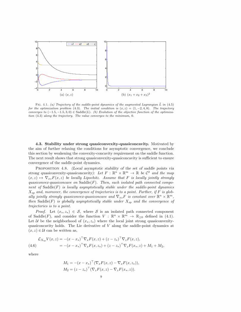
that has the same set of saddle points as L. Note that L is not strictly convex-concavebut it is globally convex-concave (this can be seen by computing its Hessian) and islinear in z. Moreover, given any (x∗, z∗) ∈ Saddle(L), we have L(x∗, z∗) = 0, and ifL(x, z∗) = L(x∗, z∗) = 0, then (x, z∗) ∈ Saddle(L). By Corollary 4.5, the trajectoriesof the saddle-point dynamics of L converge to a point in S and hence, solve theoptimization problem (4.3). Figure 4.1 illustrates this fact. Note that the point ofconvergence depends on the initial condition. •

Remark 4.7. (Relationship with results on primal-dual dynamics: II): Thework [17, Section 4] considers concave optimization problems under inequality con-straints where the objective function is not strictly concave but analyzes the conver-gence properties of a different dynamics. Specifically, the paper studies a discontin-uous dynamics based on the saddle-point information of an augmented Lagrangiancombined with a projection operator that restricts the dual variables to the nonneg-ative orthant. We have verified that, for the formulation of the concave optimizationproblem in [17] but with equality constraints, the augmented Lagrangian satisfies thehypotheses of Corollary 4.5, implying that the dynamics Xsp renders the primal-dualoptima of the problem asymptotically stable. •

8

0 2 4 6 8 10−4

−2

0

2

4

6

8

10x1 x2 x3 z

(a) (x, z)

0 2 4 6 8 100

2

4

6

8

10

(b) (x1 + x2 + x3)2

Fig. 4.1. (a) Trajectory of the saddle-point dynamics of the augmented Lagrangian L in (4.5)for the optimization problem (4.3). The initial condition is (x, z) = (1,−2, 4, 8). The trajectoryconverges to (−1.5,−1.5, 3, 0) ∈ Saddle(L). (b) Evolution of the objective function of the optimiza-tion (4.3) along the trajectory. The value converges to the minimum, 0.

4.3. Stability under strong quasiconvexity-quasiconcavity. Motivated bythe aim of further relaxing the conditions for asymptotic convergence, we concludethis section by weakening the convexity-concavity requirement on the saddle function.The next result shows that strong quasiconvexity-quasiconcavity is sufficient to ensureconvergence of the saddle-point dynamics.

Proposition 4.8. (Local asymptotic stability of the set of saddle points viastrong quasiconvexity-quasiconcavity): Let F : Rn × Rm → R be C2 and the map(x, z) 7→ ∇xzF (x, z) be locally Lipschitz. Assume that F is locally jointly stronglyquasiconvex-quasiconcave on Saddle(F ). Then, each isolated path connected compo-nent of Saddle(F ) is locally asymptotically stable under the saddle-point dynamicsXsp and, moreover, the convergence of trajectories is to a point. Further, if F is glob-ally jointly strongly quasiconvex-quasiconcave and ∇xzF is constant over Rn × Rm,then Saddle(F ) is globally asymptotically stable under Xsp and the convergence oftrajectories is to a point.

Proof. Let (x∗, z∗) ∈ S, where S is an isolated path connected componentof Saddle(F ), and consider the function V : Rn × Rm → R≥0 defined in (4.1).Let U be the neighborhood of (x∗, z∗) where the local joint strong quasiconvexity-quasiconcavity holds. The Lie derivative of V along the saddle-point dynamics at(x, z) ∈ U can be written as,

LXspV (x, z) = −(x− x∗)>∇xF (x, z) + (z − z∗)>∇zF (x, z),

= −(x− x∗)>∇xF (x, z∗) + (z − z∗)>∇zF (x∗, z) +M1 +M2,(4.6)

where

M1 = −(x− x∗)>(∇xF (x, z)−∇xF (x, z∗)),

M2 = (z − z∗)>(∇zF (x, z)−∇zF (x∗, z)).

9

Writing

∇xF (x, z)−∇xF (x, z∗) =

∫ 1

0

∇zxF (x, z∗ + t(z − z∗))(z − z∗)dt,

∇zF (x, z)−∇zF (x∗, z) =

∫ 1

0

∇xzF (x∗ + t(x− x∗), z)(x− x∗)dt,

we get

M1 +M2 = (z − z∗)>(∫ 1

0

(∇xzF (x∗ + t(x− x∗), z)

−∇xzF (x, z∗ + t(z − z∗)))dt)

(x− x∗)

≤ ‖z − z∗‖(L‖x− x∗‖+ L‖z − z∗‖)‖x− x∗‖,(4.7)

where in the inequality, we have used the fact that ∇xzF is locally Lipschitz withsome constant L > 0. From the first-order property of a strong quasiconvex function,cf. Lemma A.2, there exist constants s1, s2 > 0 such that

−(x− x∗)>∇xF (x, z∗) ≤ −s1‖x− x∗‖2,(4.8a)

(z − z∗)>∇zF (x∗, z) ≤ −s2‖z − z∗‖2,(4.8b)

for all (x, z) ∈ U . Substituting (4.7) and (4.8) into the expression for the Lie deriva-tive (4.6), we obtain

LXspV (x, z) ≤ −s1‖x− x∗‖2 − s2‖z − z∗‖2 + L‖x− x∗‖2‖z − z∗‖+ L‖x− x∗‖‖z − z∗‖2.

To conclude the proof, note that if ‖z−z∗‖ < s1L and ‖x−x∗‖ < s2

L , then LXspV (x, z) <0, which implies local asymptotic stability. The pointwise convergence follows fromLemma A.3. The global asymptotic stability can be reasoned using similar argumentsas above using the fact that here M1 +M2 = 0 because ∇xzF is constant.

In the following, we present an example where the above result is employed toexplain local asymptotic convergence. In this case, none of the results from Section 4.1and 4.2 apply, thereby justifying the importance of the above result.

Example 4.9. (Convergence for locally jointly strongly quasiconvex-quasiconcavefunction): Consider F : R× R→ R given by,

(4.9) F (x, z) = (2− e−x2

)(1 + e−z2

).

Note that F is C2 and ∇xzF (x, z) = −4xze−x2

e−z2

is locally Lipschitz. To see

this, note that the function x 7→ xe−x2

is bounded and is locally Lipschitz (as itsderivative is bounded). Further, the product of two bounded and locally Lipschitzfunctions is locally Lipschitz [32, Theorem 4.6.3] and so, (x, z) 7→ ∇xzF (x, z) is locallyLipschitz. The set of saddle points of F is Saddle(F ) = 0. Next, we show that

x 7→ f(x) = c1 − c2e−x2

, c2 > 0, is locally strongly quasiconvex at 0. Fix δ > 0 andlet x, y ∈ Bδ(0) such that f(y) ≤ f(x). Then, |y| ≤ |x| and

maxf(x), f(y) − f(λx+ (1− λ)y)− sλ(1− λ)(x− y)2

= c2(−e−x2

+ e−(λx+(1−λ)y)2)− sλ(1− λ)(x− y)2

10

= c2e−x2

(−1 + ex2−(λx+(1−λ)y)2)− sλ(1− λ)(x− y)2

≥ c2e−x2

(x2 − (λx+ (1− λ)y)2)− sλ(1− λ)(x− y)2

= (1− λ)(x− y)(c2e−x2

(x+ y) + λ(x− y)(c2e−x2

− s))≥ 0,

for s ≤ c2e−δ2 , given the fact that |y| ≤ |x|. Therefore, f is locally strongly qua-

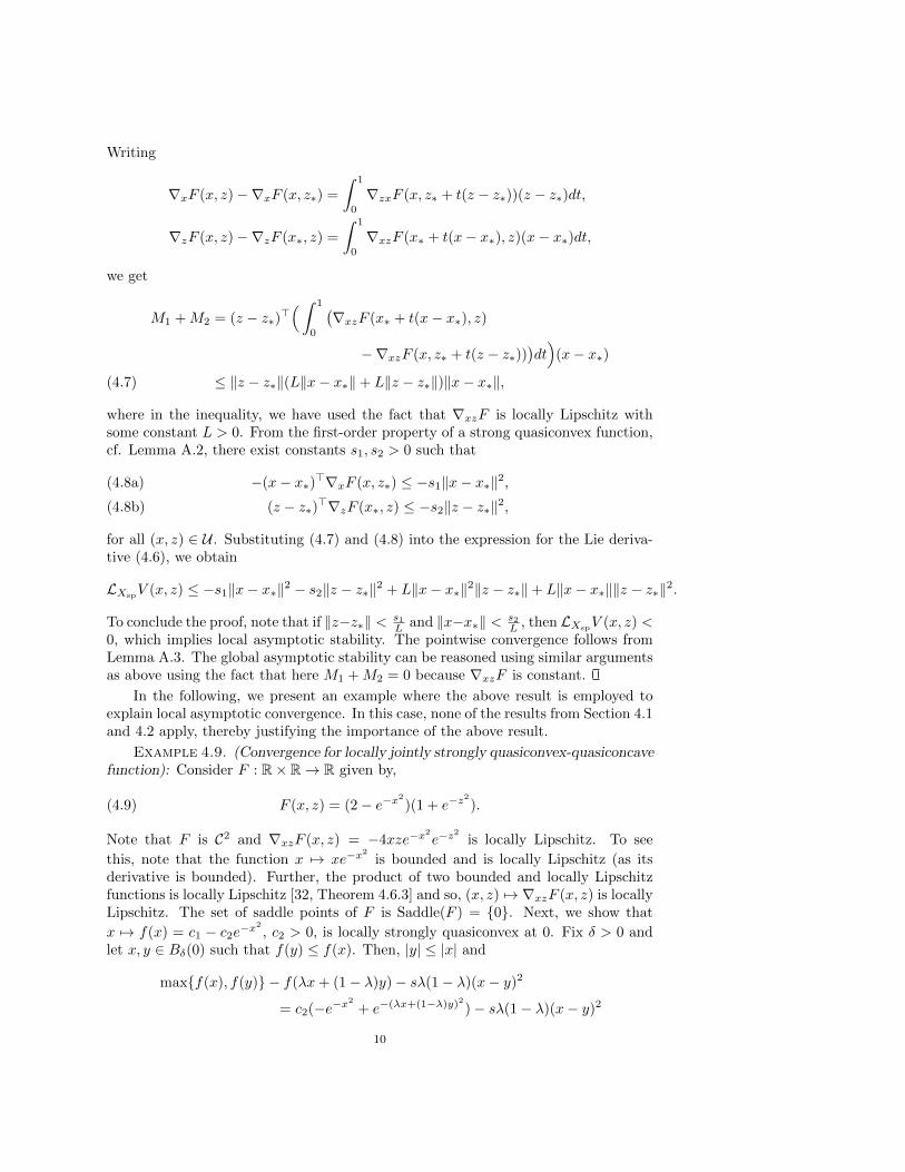
siconvex and so −f is locally strongly quasiconcave. Using these facts, we deducethat F is locally jointly strongly quasiconvex-quasiconcave. Thus, the hypotheses ofProposition 4.8 are met, implying local asymptotic stability of Saddle(F ) under thesaddle-point dynamics. Figure 4.2 illustrates this fact in simulation. Note that Fdoes not satisfy the conditions outlined in results of Section 4.1 and 4.2. •

0 1 2 3 40

0.1

0.2

0.3

0.4

0.5x z

(a) (x, z)

0 1 2 3 40

0.02

0.04

0.06

0.08

0.1

0.12

0.14

0.16

(b) (x2 + z2)/2

Fig. 4.2. (a) Trajectory of the saddle-point dynamics for F given in (4.9). The initial conditionis (x, z) = (0.5, 0.2). The trajectory converges to the saddle point (0, 0). (b) Evolution of the functionV along the trajectory.

5. Convergence analysis for general saddle functions. We study here theconvergence properties of the saddle-point dynamics associated to functions that arenot convex-concave. Our first result explores conditions for local asymptotic stabilitybased on the linearization of the dynamics and properties of the eigenstructure of theJacobian matrices. In particular, we assume that Xsp is piecewise C2 and that the setof limit points of the Jacobian of Xsp at any saddle point have a common kernel andnegative real parts for the nonzero eigenvalues. The proof is a direct consequence ofProposition A.5.

Proposition 5.1. (Local asymptotic stability of manifold of saddle points vialinearization – piecewise C3 saddle function): Given F : Rn × Rm → R, let S ⊂Saddle(F ) be a p-dimensional submanifold of saddle points. Assume that F is C1

with locally Lipschitz gradient on a neighborhood of S and that the vector field Xsp ispiecewise C2. Assume that at each (x∗, z∗) ∈ S, the set of matrices A∗ ⊂ Rn+m×n+m

defined as

A∗ = limk→∞

DXsp(xk, zk) | (xk, zk)→ (x, z), (xk, zk) ∈ Rn+m \ ΩXsp,

where ΩXsp is the set of points where Xsp is not differentiable, satisfies the following:

11

(i) there exists an orthogonal matrix Q ∈ Rn+m×n+m such that

(5.1) Q>AQ =

[0 0

0 A

],

for all A ∈ A∗, where A ∈ Rn+m−p×n+m−p,(ii) the nonzero eigenvalues of the matrices in A∗ have negative real parts,

(iii) there exists a positive definite matrix P ∈ Rn+m−p×n+m−p such that

A>P + PA ≺ 0,

for all A obtained by applying transformation (5.1) on each A ∈ A∗.Then, S is locally asymptotically stable under (A.7) and the trajectories converge toa point in S.

When F is sufficiently smooth, we can refine the above result as follows.

Corollary 5.2. (Local asymptotic stability of manifold of saddle points vialinearization – C3 saddle function): Given F : Rn ×Rm → R, let S ⊂ Saddle(F ) be ap-dimensional manifold of saddle points. Assume F is C3 on a neighborhood of S andthat the Jacobian of Xsp at each point in S has no eigenvalues in the imaginary axisother than 0, which is semisimple with multiplicity p. Then, S is locally asymptoticallystable under the saddle-point dynamics Xsp and the trajectories converge to a point.

Proof. Since F is C3, the map Xsp is C2 and so, the limit point of Jacobianmatrices at a saddle point (x∗, z∗) ∈ S is the Jacobian at that point itself, that is,

DXsp =

[−∇xxF −∇xzF∇zxF ∇zzF

](x∗,z∗)

.

From the definition of saddle point, we have ∇xxF (x∗, z∗) 0 and ∇zzF (x∗, z∗) 0.In turn, we obtain DXsp + DX>sp 0, and since Re(λi(DXsp)) ≤ λmax( 1

2 (DXsp +

DX>sp)) [4, Fact 5.10.28], we deduce that Re(λi(DXsp)) ≤ 0. The statement nowfollows from Proposition 5.1 using the fact that the properties of the eigenvalues ofDXsp shown here imply existence of an orthonormal transformation leading to a formof DXsp that satisfies assumptions (i)-(iii) of Proposition 5.1.

Next, we provide a sufficient condition under which the Jacobian of Xsp for asaddle function F that is linear in its second argument satisfies the hypothesis ofCorollary 5.2 regarding the lack of eigenvalues on the imaginary axis other than 0.

Lemma 5.3. (Sufficient condition for absence of imaginary eigenvalues of theJacobian of Xsp): Let F : Rn × Rm → R be C2 and linear in the second argument.Then, the Jacobian of Xsp at any saddle point (x∗, z∗) of F has no eigenvalues on theimaginary axis except for 0 if range(∇zxF (x∗, z∗)) ∩ null(∇xxF (x∗, z∗)) = 0.

Proof. The Jacobian of Xsp at a saddle point (x∗, z∗) for a saddle function F thatis linear in z is given as

DXsp =

[A B−B> 0

],

where A = −∇xxF (x∗, z∗) and B = −∇zxF (x∗, z∗). We reason by contradiction. Letiλ, λ 6= 0 be an imaginary eigenvalue of DXsp with the corresponding eigenvectora+ ib. Let a = (a1; a2) and b = (b1; b2) where a1, b1 ∈ Rn and a2, b2 ∈ Rm. Then the

12

real and imaginary parts of the condition DXsp(a+ ib) = (iλ)(a+ ib) yield

Aa1 +Ba2 = −λb1, −B>a1 = −λb2,(5.2)

Ab1 +Bb2 = λa1, −B>b1 = λa2.(5.3)

Pre-multiplying the first equation of (5.2) with a>1 gives a>1 Aa1 + a>1 Ba2 = −λa>1 b1.Using the second equation of (5.2), we get a>1 Aa1 = −λ(a>1 b1 + a>2 b2). A similarprocedure for the set of equations in (5.3) gives b>1 Ab1 = λ(a>1 b1 + a>2 b2). Theseconditions imply that a>1 Aa1 = −b>1 Ab1. Since A is negative semi-definite, we obtaina1, b1 ∈ null(A). Note that a1, b1 6= 0, because otherwise it would mean that a = b = 0.Further, using this fact in the first equations of (5.2) and (5.3), respectively, we get

Ba2 = −λb1, Bb2 = λa1.

That is, a1, b1 ∈ range(B), a contradiction.

The following example illustrates an application of the above results to a noncon-vex constrained optimization problem.

Example 5.4. (Saddle-point dynamics for nonconvex optimization): Considerthe following constrained optimization on R3,

minimize (‖x‖ − 1)2,(5.4a)

subject to x3 = 0.5,(5.4b)

where x = (x1, x2, x3) ∈ R3. The optimizers are x ∈ R3 | x3 = 0.5, x21 + x2

2 = 0.75.The Lagrangian L : R3 × R→ R is given by

L(x, z) = (‖x‖ − 1)2 + z(x3 − 0.5),

and its set of saddle points is the one-dimensional manifold Saddle(L) = (x, z) ∈R3 × R | x3 = 0.5, x2

1 + x22 = 0.75, z = 0. The saddle-point dynamics of L takes the

form

x = −2(

1− 1

‖x‖

)x− [0, 0, z]>,(5.5a)

z = x3 − 0.5.(5.5b)

Note that Saddle(L) is nonconvex and that L is nonconvex in its first argument onany neighborhood of any saddle point. Therefore, results that rely on the convexity-concavity properties of L are not applicable to establish the asymptotic convergenceof (5.5) to the set of saddle points. This can, however, be established throughCorollary 5.2 by observing that the Jacobian of Xsp at any point of Saddle(L) has0 as an eigenvalue with multiplicity one and the rest of the eigenvalues are noton the imaginary axis. To show this, consider (x∗, z∗) ∈ Saddle(L). Note that

DXsp(x∗, z∗) =

[−2x>∗ x∗ −e3

e>3 0

], where e3 = [0, 0, 1]>. One can deduce from this

that v ∈ null(DXsp(x∗, z∗)) if and only if x>∗ [v1, v2, v3]> = 0, v3 = 0, and v4 = 0.These three conditions define a one-dimensional space and so 0 is an eigenvalue ofDXsp(x∗, z∗) with multiplicity 1. To show that the rest of eigenvalues do not lie onthe imaginary axis, we show that the hypotheses of Lemma 5.3 are met. At anysaddle point (x∗, z∗), we have ∇zxL(x∗, z∗) = e3 and ∇xxL(x∗, z∗) = 2x>∗ x∗. If

13

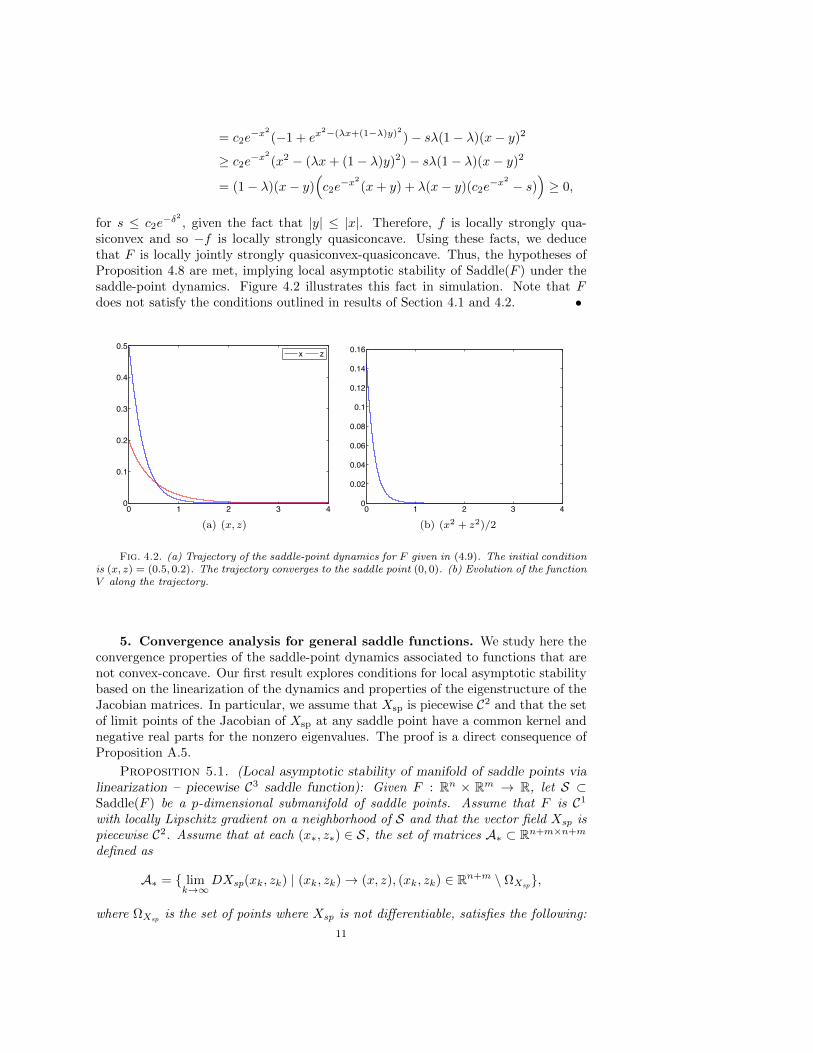
v ∈ range(∇zxL(x∗, z∗))∩null(∇xxL(x∗, z∗)) then v = [0, 0, λ]>, λ ∈ R, and x>∗ v = 0.Since (x∗)3 = 0.5, we get λ = 0 and hence, the hypotheses of Lemma 5.3 are satisfied.Figure 5.1 illustrates in simulation the convergence of the trajectories to a saddlepoint. The point of convergence depends on the initial condition. •

0 50 100 150−0.5

0

0.5

1x1 x2 x3 z

(a) (x, z)

0 50 100 1500

0.005

0.01

0.015

0.02

0.025

(b) (x1 + x2 + x3)2

Fig. 5.1. (a) Trajectory of the saddle-point dynamics (5.5) for the Lagrangian of the con-strained optimization problem (5.4). The initial condition is (x, z) = (0.9, 0.7, 0.2, 0.3). The tra-jectory converges to (0.68, 0.53, 0.50, 0) ∈ Saddle(L). (b) Evolution of the objective function of theoptimization (5.4) along the trajectory. The value converges to the minimum, 0.

There are functions that do not satisfy the hypotheses of Proposition 5.1 whosesaddle-point dynamics still seems to enjoy local asymptotic convergence properties.As an example, consider the function F : R2 × R→ R,

F (x, z) = (‖x‖ − 1)4 − z2‖x‖2,(5.6)

whose set of saddle points is the one-dimensional manifold Saddle(F ) = (x, z) ∈R2 × R | ‖x‖ = 1, z = 0. The Jacobian of the saddle-point dynamics at any (x, z) ∈Saddle(F ) has −2 as an eigenvalue and 0 as the other eigenvalue, with multiplicity2, which is greater than the dimension of S (and therefore Proposition 5.1 cannotbe applied). Simulations show that the trajectories of the saddle-point dynamicsasymptotically approach Saddle(S) if the initial condition is close enough to this set.Our next result allows us to formally establish this fact by studying the behavior ofthe function along the proximal normals to Saddle(F ).

Proposition 5.5. (Asymptotic stability of manifold of saddle points via prox-imal normals): Let F : Rn × Rm → R be C2 and S ⊂ Saddle(F ) be a closed set.Assume there exist constants λM , k1, k2, α1, β1 > 0 and Lx, Lz, α2, β2 ≥ 0 such thatthe following hold

(i) either Lx = 0 or α1 ≤ α2 + 1,(ii) either Lz = 0 or β1 ≤ β2 + 1,

(iii) for every (x∗, z∗) ∈ S and every proximal normal η = (ηx, ηz) ∈ Rn × Rm toS at (x∗, z∗) with ‖η‖ = 1, the functions

[0, λM ) 3 λ 7→ F (x∗ + ληx, z∗),

[0, λM ) 3 λ 7→ F (x∗, z∗ + ληz),

14

are convex and concave, respectively, with

F (x∗ + ληx, z∗)− F (x∗, z∗) ≥ k1‖ληx‖α1 ,(5.7a)

F (x∗, z∗ + ληz)− F (x∗, z∗) ≤ −k2‖ληz‖β1 ,(5.7b)

and, for all λ ∈ [0, λM ) and all t ∈ [0, 1],

(5.8) ‖∇xzF (x∗ + tληx, z∗ + ληz)−∇xzF (x∗ + ληx, z∗ + tληz)‖≤ Lx‖ληx‖α2 + Lz‖ληz‖β2 .

Then, S is locally asymptotically stable under the saddle-point dynamics Xsp. More-over, the convergence of the trajectories is to a point if every point of S is stable. Theconvergence is global if, for every λM ∈ R≥0, there exist k1, k2, α1, β1 > 0 such that theabove hypotheses (i)-(iii) are satisfied by these constants along with Lx = Lz = 0.

Proof. Our proof is based on showing that there exists λ ∈ (0, λM ] such thatthe distance function dS decreases monotonically and converges to zero along thetrajectories of Xsp that start in S +Bλ(0). From (2.2),

∂d2S(x, z) = co2(x− x∗; z − z∗) | (x∗, z∗) ∈ projS(x, z).

Following [12], we compute the set-valued Lie derivative of d2S along Xsp, denoted

LXspd2S : Rn × Rm ⇒ R, as

LXspd2S(x, z) = co−2(x− x∗)>∇xF (x, z)+

2(z − z∗)>∇zF (x, z) | (x∗, z∗) ∈ projS(x, z).

Since d2S is globally Lipschitz and regular, cf. Section 2.2, the evolution of the function

d2S along any trajectory t 7→ (x(t), z(t)) of (3.1) is differentiable at almost all t ∈ R≥0,

and furthermore, cf. [12, Proposition 10],

d

dt(d2S(x(t), z(t)) ∈ LXsp

d2S(x(t), z(t))

for almost all t ∈ R≥0. Therefore, our goal is to show that maxLXspd2S(x, z) < 0 for

all (x, z) ∈ (S + Bλ(0)) \ S for some λ ∈ (0, λM ]. Let (x, z) ∈ S + BλM(0) and take

(x∗, z∗) ∈ projS(x, z). By definition, there exists a proximal normal η = (ηx, ηz) toS at (x∗, z∗) with ‖η‖ = 1 and x = x∗ + ληx, z = z∗ + ληz, and λ ∈ [0, λM ). Let2ξ ∈ LXsp

d2S(x, z) denote

(5.9) ξ = −(x− x∗)>∇xF (x, z) + (z − z∗)>∇zF (x, z).

Writing

∇xF (x, z) = ∇xF (x, z∗) +

∫ 1

0

∇zxF (x, z∗ + t(z − z∗))(z − z∗)dt,

∇zF (x, z) = ∇zF (x∗, z) +

∫ 1

0

∇xzF (x∗ + t(x− x∗), z)(x− x∗)dt,

15

and substituting in (5.9) we get

ξ = −(x− x∗)>∇xF (x, z∗) + (z − z∗)>∇zF (x∗, z) + (z − z∗)>M(x− x∗),(5.10)

where M =∫ 1

0(∇xzF (x∗ + t(x − x∗), z) − ∇xzF (x, z∗ + t(z − z∗)))dt. Using the

convexity and concavity along the proximal normal and applying the bounds (5.7),we obtain

−(x− x∗)>∇xF (x, z∗) ≤ F (x∗, z∗)− F (x, z∗) ≤ −k1‖ληx‖α1 ,(5.11a)

(z − z∗)>∇zF (x∗, z) ≤ F (x∗, z)− F (x∗, z∗) ≤ −k2‖ληz‖β1 .(5.11b)

On the other hand, using (5.8), we bound M by

(5.12) ‖M‖ ≤ Lx‖ληx‖α2 + Lz‖ληz‖β2 .

Using (5.11) and (5.12) in (5.10), and rearranging the terms yields

ξ ≤(−k1‖ληx‖α1 + Lx‖ληx‖α2+1‖ληz‖

)+(−k2‖ληz‖β1 + Lz‖ληz‖β2+1‖ληx‖

).

If Lx = 0, then the first parenthesis is negative whenever ληx 6= 0 (i.e., x 6= x∗).If Lx 6= 0 and α1 ≤ α2 + 1, then for ‖ληx‖ < 1 and ‖ληz‖ < min(1, k1/Lx), thefirst parenthesis is negative whenever ληx 6= 0. Analogously, the second parenthesisis negative for z 6= z∗ if either Lz = 0 or β1 ≤ β2 + 1 with ‖ληz‖ < 1 and ‖ληx‖ <min(1, k2/Lz). Thus, if λ < min1, k1/Lx, k2/Lz (excluding from the min operationthe elements that are not well defined due to the denominator being zero), thenhypotheses (i)-(ii) imply that ξ < 0 whenever (x, z) 6= (x∗, z∗). Moreover, since(x∗, z∗) ∈ projS(x, z) was chosen arbitrarily, we conclude that maxLXspd

2S(x, z) < 0

for all (x, z) ∈ S +Bλ(0) where λ ∈ (0, λM ] satisfies λ < min1, k1/Lx, k2/Lz. Thisproves the local asymptotic stability. Finally, convergence to a point follows fromLemma A.3 and global convergence follows from the analysis done above.

Intuitively, the hypotheses of Proposition 5.5 imply that along the proximal nor-mal to the saddle set, the convexity (resp. concavity) in the x-coordinate (resp.z-coordinate) is ‘stronger’ than the influence of the x- and z-dynamics on each other,represented by the off-diagonal Hessian terms. When this coupling is absent (i.e.,∇xzF ≡ 0), the x- and z-dynamics are independent of each other and they func-tion as individually aiming to minimize (resp. maximize) a function of one variable,thereby, reaching a saddle point. Note that the assumptions of Proposition 5.5 donot imply that F is locally convex-concave. As an example, the function in (5.6) isnot convex-concave in any neighborhood of any saddle point but we show next that itsatisfies the assumptions of Proposition 5.5, establishing local asymptotic convergenceof the respective saddle-point dynamics.

Example 5.6. (Convergence analysis via proximal normals): Consider the func-tion F defined in (5.6). Consider a saddle point (x∗, z∗) = (cos θ, sin θ, 0) ∈ Saddle(F ),where θ ∈ [0, 2π). Let

η = (ηx, ηz) = ((a1 cos θ, a1 sin θ), a2),

with a1, a2 ∈ R and a21 + a2

2 = 1, be a proximal normal to Saddle(F ) at (x∗, z∗).Note that the function λ 7→ F (x∗ + ληx, z∗) = (λa1)4 is convex, satisfying (5.7a)with k1 = 1 and α1 = 4. The function λ 7→ F (x∗, z∗ + ληz) = −(λa2)2 is concave,

16

satisfying (5.7b) with k2 = 1, β1 = 2. Also, given any λM > 0 and for all t ∈ [0, 1],we can write

‖∇xzF (x∗ + tληx, z∗ + ληz)−∇xzF (x∗ + ληx, z∗ + tληz)‖= ‖ − 4(λa2)(1 + tλa1)

(cos θsin θ

)+ 4(tλa2)(1 + λa1)

(cos θsin θ

)‖,

≤ ‖4(λa2)(1 + tλa1)− 4(tλa2)(1 + λa1)‖,≤ 8(1 + λa1)(λa2) ≤ Lz(λa2),

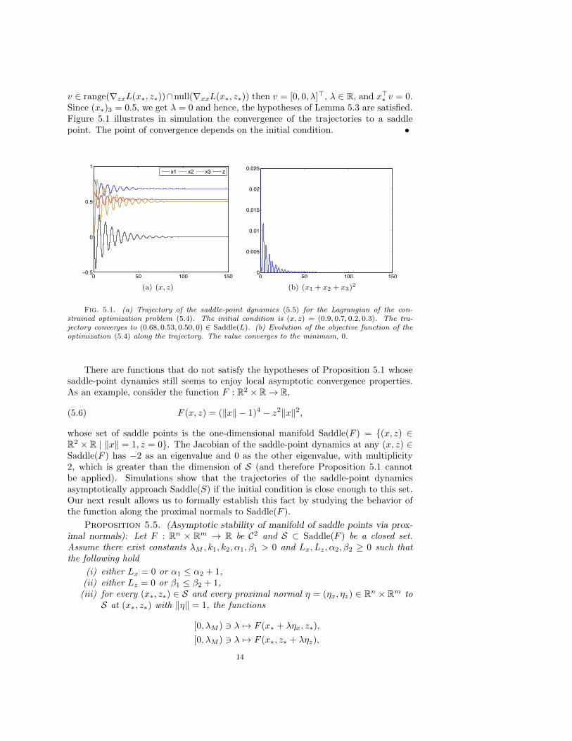
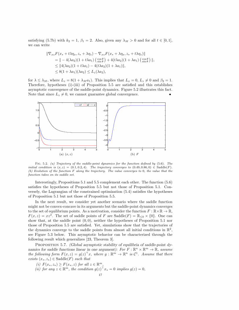
for λ ≤ λM , where Lz = 8(1 + λMa1). This implies that Lx = 0, Lz 6= 0 and β2 = 1.Therefore, hypotheses (i)-(iii) of Proposition 5.5 are satisfied and this establishesasymptotic convergence of the saddle-point dynamics. Figure 5.2 illustrates this fact.Note that since Lz 6= 0, we cannot guarantee global convergence. •

0 1 2 3 4 5−1

−0.5

0

0.5

1

1.5

2x1 x2 z

(a) (x, z)

0 1 2 3 4 5

−4

−3.5

−3

−2.5

−2

−1.5

−1

−0.5

0

(b) F

Fig. 5.2. (a) Trajectory of the saddle-point dynamics for the function defined by (5.6). Theinitial condition is (x, z) = (0.1, 0.2, 4). The trajectory converges to (0.49, 0.86, 0) ∈ Saddle(F ).(b) Evolution of the function F along the trajectory. The value converges to 0, the value that thefunction takes on its saddle set.

Interestingly, Propositions 5.1 and 5.5 complement each other. The function (5.6)satisfies the hypotheses of Proposition 5.5 but not those of Proposition 5.1. Con-versely, the Lagrangian of the constrained optimization (5.4) satisfies the hypothesesof Proposition 5.1 but not those of Proposition 5.5.

In the next result, we consider yet another scenario where the saddle functionmight not be convex-concave in its arguments but the saddle-point dynamics convergesto the set of equilibrium points. As a motivation, consider the function F : R×R→ R,F (x, z) = xz2. The set of saddle points of F are Saddle(F ) = R≤0 × 0. One canshow that, at the saddle point (0, 0), neither the hypotheses of Proposition 5.1 northose of Proposition 5.5 are satisfied. Yet, simulations show that the trajectories ofthe dynamics converge to the saddle points from almost all initial conditions in R2,see Figure 5.3 below. This asymptotic behavior can be characterized through thefollowing result which generalizes [23, Theorem 3].

Proposition 5.7. (Global asymptotic stability of equilibria of saddle-point dy-namics for saddle functions linear in one argument): For F : Rn × Rm → R, assumethe following form F (x, z) = g(z)>x, where g : Rm → Rn is C1. Assume that thereexists (x∗, z∗) ∈ Saddle(F ) such that

(i) F (x∗, z∗) ≥ F (x∗, z) for all z ∈ Rm,(ii) for any z ∈ Rm, the condition g(z)>x∗ = 0 implies g(z) = 0,

17

(iii) any trajectory of Xsp is bounded.

Then, all trajectories of the saddle-point dynamics Xsp converge asymptotically to theset of equilibrium points of Xsp.

Proof. Consider the function V : Rn × Rm → R,

V (x, z) = −x>∗ x.

The Lie derivative of V along the saddle-point dynamics Xsp is

LXspV (x, z) = x>∗ ∇xF (x, z) = x>∗ g(z) = F (x∗, z) ≤ F (x∗, z∗) = 0,(5.13)

where in the inequality we have used assumption (i), and F (x∗, z∗) = 0 is implied bythe definition of the saddle point, that is, ∇xF (x∗, z∗) = g(z∗) = 0. Now considerany trajectory t 7→ (x(t), z(t)), (x(0), z(0)) ∈ Rn ×Rm of Xsp. Since the trajectory isbounded by assumption (iii), the application of the LaSalle Invariance Principle [24,Theorem 4.4] yields that the trajectory converges to the largest invariant set Mcontained in (x, z) ∈ Rn × Rm | LXsp

V (x, z) = 0, which from (5.13) is equalto the set (x, z) ∈ Rn × Rm | F (x∗, z) = 0. Let (x, z) ∈ M. Then, we haveF (x∗, z) = g(z)>x∗ = 0 and by hypotheses (ii) we get g(z) = 0. Therefore, if(x, z) ∈ M then g(z) = 0. Consider the trajectory t 7→ (x(t), z(t)) of Xsp with(x(0), z(0)) = (x, z) which is contained in M. Then, along the trajectory we have

x(t) = −∇xF (x(t), z(t)) = −g(z(t)) = 0

Further, note that along this trajectory we have g(z(t)) = 0 for all t ≥ 0. Thus,ddtg(z(t)) = 0 for all t ≥ 0, which implies that

d

dtg(z(t)) = Dg(z(t))z(t) = Dg(z(t))Dg(z(t))>x = 0.

From the above expression we deduce that z(t) = Dg(z(t))>x = 0. This can beseen from the fact that Dg(z(t))Dg(z(t))>x = 0 implies x>Dg(z(t))Dg(z(t))>x =(Dg(z(t))>x)2 = 0. From the above reasoning, we conclude that (x, z) is an equilib-rium point of Xsp.

The proof of Proposition 5.7 hints at the fact that hypothesis (ii) can be omittedif information about other saddle points of F is known. Specifically, consider the case

where n saddle points (x(1)∗ , z

(1)∗ ), . . . , (x

(n)∗ , z

(n)∗ ) of F exist, each satisfying hypothesis

(i) of Proposition 5.7 and such that the vectors x(1)∗ , . . . , x

(n)∗ are linearly independent.

In this scenario, for those points z ∈ Rm such that g(z)>x(i)∗ = 0 for all i ∈ 1, . . . , n

(as would be obtained in the proof), the linear independence of x(i)∗ ’s already implies

that g(z) = 0, making hypothesis (ii) unnecessary.

Corollary 5.8. (Almost global asymptotic stability of saddle points for saddlefunctions linear in one argument): If, in addition to the hypotheses of Proposition 5.7,the set of equilibria of Xsp other than those belonging to Saddle(F ) are unstable, thenthe trajectories of Xsp converge asymptotically to Saddle(F ) from almost all initialconditions (all but the unstable equilibria). Moreover, if each point in Saddle(F ) isstable under Xsp, then Saddle(F ) is almost globally asymptotically stable under thesaddle-point dynamics Xsp and the trajectories converge to a point in Saddle(F ).

Next, we illustrate how the above result can be applied to the motivating example

18

given before Proposition 5.7 to infer almost global convergence of the trajectories.

Example 5.9. (Convergence for saddle functions linear in one argument): Con-sider again F (x, z) = xz2 with Saddle(F ) = (x, z) ∈ R×R | x ≤ 0 and z = 0. Pick(x∗, z∗) = (−1, 0). One can verify that this saddle point satisfies the hypotheses (i)and (ii) of Proposition 5.7. Moreover, along any trajectory of the saddle-point dy-

namics for F , the function x2 + z2

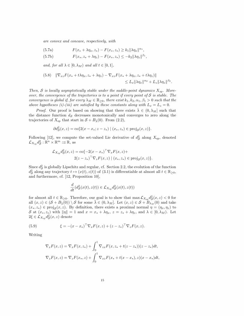
2 is preserved, which implies that all trajectoriesare bounded. One can also see that the equilibria of the saddle-point dynamics thatare not saddle points, that is the set R>0 ×0, are unstable. Therefore, from Corol-lary 5.8, we conclude that the trajectories of the saddle-point dynamics asymptoticallyconverge to the set of saddle points from almost all initial conditions. Figure 5.3 il-lustrates these observations. •

0 1 2 3 4−8

−6

−4

−2

0

2

4

6

8

10x z

(a) (x, z)

0 1 2 3 4−200

−150

−100

−50

0

50

100

150

200

(b) F (c) Vector field Xsp

Fig. 5.3. (a) Trajectory of the saddle-point dynamics for the function F (x, z) = xz2. Theinitial condition is (x, z) = (5, 5). The trajectory converges to (−6.13, 0) ∈ Saddle(F ). (b) Evolutionof the function F along the trajectory. The value converges to 0, the value that the function takeson its saddle set. (c) The vector field Xsp, depicting that the set of saddle points are attractive whilethe other equilibrium points R>0 × 0 are unstable.

6. Conclusions. We have studied the asymptotic stability of the saddle-pointdynamics associated to a continuously differentiable function. We have identified aset of complementary conditions under which the trajectories of the dynamics areproved to converge to the set of saddle points of the saddle function and, whereverfeasible, we have also established global stability guarantees and convergence to apoint in the set. Our first class of convergence results is based on the convexity-concavity properties of the saddle function. In the absence of these properties, oursecond class of results explore, respectively, the existence of convergence guaranteesusing linearization techniques, the properties of the saddle function along proximalnormals to the set of saddle points, and the linearity properties of the saddle functionin one variable. For the linearization result, borrowing ideas from center manifoldtheory, we have established a general stability result of a manifold of equilibria for apiecewise twice continuously differentiable vector field. Several examples throughoutthe paper highlight the connections among the results and illustrate their applica-bility, in particular, for finding the primal-dual solutions of constrained optimizationproblems. Future work will study the robustness properties of the dynamics againstdisturbances, investigate the characterization of the rate of convergence, generalizethe results to the case of nonsmooth functions (where the associated saddle-point dy-namics takes the form of a differential inclusion involving the generalized gradient ofthe function), and explore the application to optimization problems with inequalityconstraints. We also plan to build on our results to synthesize distributed algorithmicsolutions for various networked optimization problems in power networks.

19

REFERENCES

[1] P.-A. Absil and K. Kurdyka, On the stable equilibrium points of gradient systems, Systems& Control Letters, 55 (2006), pp. 573–577.

[2] K. Arrow, L. Hurwitz, and H. Uzawa, Studies in Linear and Non-Linear Programming,Stanford University Press, Stanford, California, 1958.

[3] T. Basar and G. Oldser, Dynamic Noncooperative Game Theory, Academic Press, 1982.[4] D. S. Bernstein, Matrix Mathematics, Princeton University Press, Princeton, NJ, 2005.[5] S. P. Bhat and D. S. Bernstein, Nontangency-based Lyapunov tests for convergence and

stability in systems having a continuum of equilibria, SIAM Journal on Control and Opti-mization, 42 (2003), pp. 1745–1775.

[6] S. Boyd and L. Vandenberghe, Convex Optimization, Cambridge University Press, 2004.[7] J. Carr, Applications of Centre Manifold Theory, Springer, New York, 1982.[8] A. Cherukuri and J. Cortes, Asymptotic stability of saddle points under the saddle-point

dynamics, in American Control Conference, Chicago, IL, July 2015, pp. 2020–2025.[9] A. Cherukuri, E. Mallada, and J. Cortes, Asymptotic convergence of primal-dual dynam-

ics, Systems & Control Letters, 87 (2016), pp. 10–15.[10] F. H. Clarke, Optimization and Nonsmooth Analysis, Canadian Mathematical Society Series

of Monographs and Advanced Texts, Wiley, 1983.[11] F. H. Clarke, Y. Ledyaev, R. J. Stern, and P. R. Wolenski, Nonsmooth Analysis and

Control Theory, vol. 178 of Graduate Texts in Mathematics, Springer, 1998.[12] J. Cortes, Discontinuous dynamical systems - a tutorial on solutions, nonsmooth analysis,

and stability, IEEE Control Systems Magazine, 28 (2008), pp. 36–73.[13] R. Dorfman, P. A. Samuelson, and R. Solow, Linear programming in economic analysis,

McGraw Hill, New York, Toronto, and London, 1958.[14] G. Droge and M. Egerstedt, Proportional integral distributed optimization for dynamic

network topologies, in American Control Conference, Portland, OR, June 2014, pp. 3621–3626.

[15] J. Dugundji, Topology, Allyn and Bacon, Inc., Boston, MA, 1966.[16] H. B. Durr and C. Ebenbauer, A smooth vector field for saddle point problems, in IEEE

Conf. on Decision and Control, Orlando, Florida, Dec. 2011, pp. 4654–4660.[17] D. Feijer and F. Paganini, Stability of primal-dual gradient dynamics and applications to

network optimization, Automatica, 46 (2010), pp. 1974–1981.[18] B. Gharesifard and J. Cortes, Distributed continuous-time convex optimization on weight-

balanced digraphs, IEEE Transactions on Automatic Control, 59 (2014), pp. 781–786.[19] D. Henry, Geometric Theory of Semilinear Parabolic Equations, vol. 840 of Lecture Notes in

Mathematics, Springer, New York, 1981.[20] W. M. Hirsch and S. Smale, Differential Equations, Dynamical Systems and Linear Algebra,

Academic Press, 1974.[21] T. Holding and I. Lestas, On the convergence of saddle points of concave-convex functions,

the gradient method and emergence of oscillations, in IEEE Conf. on Decision and Control,Los Angeles, CA, 2014, pp. 1143–1148.

[22] M. V. Jovanovic, A note on strongly convex and quasiconvex functions, Mathematical Notes,60 (1996), pp. 584–585.

[23] V. A. Kamenetskiy and Y. S. Pyatnitskiy, An iterative method of lyapunov function con-struction for differential inclusions, Systems & Control Letters, 8 (1987), pp. 445–451.

[24] H. K. Khalil, Nonlinear Systems, Prentice Hall, 3 ed., 2002.[25] T. Kose, Solutions of saddle value problems by differential equations, Econometrica, 24 (1956),

pp. 59–70.[26] X. Ma and N. Elia, A distributed continuous-time gradient dynamics approach for the active

power loss minimizations, in Allerton Conf. on Communications, Control and Computing,Monticello, IL, Oct. 2013, pp. 100–106.

[27] A. Nedic and A. Ozdaglar, Subgradient methods for saddle-point problems, Journal of Opti-mization Theory & Applications, 142 (2009), pp. 205–228.

[28] J. Palis, Jr. and W. de Melo, Geometric Theory of Dynamical Systems, Springer, New York,1982.

[29] L. J. Ratliff, S. A. Burden, and S. S. Sastry, Characterization and computation of localNash equilibrium in continuous games, in Allerton Conf. on Communications, Control andComputing, Monticello, IL, Oct. 2013.

[30] D. Richert and J. Cortes, Robust distributed linear programming, IEEE Transactions onAutomatic Control, 60 (2015), pp. 2567–2582.

[31] , Distributed bargaining in dyadic-exchange networks, IEEE Transactions on Control of

20

Network Systems, 3 (2016). To appear.[32] H. H. Sohrab, Basic Real Analysis, Birkhauser, Boston, MA, 2003.[33] J. Wang and N. Elia, A control perspective for centralized and distributed convex optimization,

in IEEE Conf. on Decision and Control, Orlando, Florida, 2011, pp. 3800–3805.[34] X. Zhang and A. Papachristodoulou, A real-time control framework for smart power net-

works with star topology, in American Control Conference, Washington, DC, June 2013,pp. 5062–5067.

[35] C. Zhao, U. Topcu, N. Li, and S. Low, Design and stability of load-side primary frequencycontrol in power systems, IEEE Transactions on Automatic Control, 59 (2014), pp. 1177–1189.

Appendix. This section contains some auxiliary results for our convergence anal-ysis in Sections 4 and 5. Our first result establishes the constant value of the saddlefunction over its set of (local) saddle points.

Lemma A.1. (Constant function value over saddle points): For F : Rn×Rm → Rcontinuously differentiable, let S ⊂ Saddle(F ) be a path connected set. If F is locallyconvex-concave on S, then F|S is constant.

Proof. We start by considering the case when S is compact. Given (x, z) ∈ S,let δ(x, z) > 0 be such that Bδ(x,z)(x, z) ⊂ (Ux × Uz) ∩ U , where Ux and Uz areneighborhoods where the saddle property (2.3) holds and U is the neighborhood of(x, z) where local convexity-concavity holds (cf. Section 2.3). This defines a coveringof S by open sets as

S ⊂ ∪(x,z)∈SBδ(x,z)(x, z).

Since S is compact, there exist a finite number of points (x1, z1), (x2, z2), . . . , (xn, zn)in S such that ∪ni=1Bδ(xi,zi)(xi, zi) covers S. For convenience, denote Bδ(xi,zi)(xi, zi)by Bi. Next, we show that F|S∩Bi

is constant for all i ∈ 1, . . . , n. To see this, let(x, z) ∈ S ∩Bi. From (2.3), we have

(A.1) F (xi, z) ≤ F (xi, zi) ≤ F (x, zi).

From the convexity of x 7→ F (x, z) over U ∩ (Rn × z), (cf. definition of localconvexity-concavity in Section 2.3), and the fact that ∇xF (x, z) = 0, we obtainF (xi, z) ≥ F (x, z) + (xi − x)>∇xF (x, z) = F (x, z). Similarly, using the concavity ofz 7→ F (x, z), we get F (x, zi) ≤ F (x, z). These inequalities together with (A.1) yield

F (xi, zi) ≤ F (x, zi) ≤ F (x, z) ≤ F (xi, z) ≤ F (xi, zi).

That is, F (x, z) = F (xi, zi) and hence F|S∩Biis constant. Using this reasoning, if

S ∩Bi∩Bj 6= ∅ for any i, j ∈ 1, . . . , n, then F|S∩(Bi∪Bj) is constant. Using that S ispath connected, the fact [15, p. 117] states that, for any two points (xl, zl), (xm, zm) ∈S, there exist distinct members i1, i2, . . . , ik of the set 1, . . . , n such that (xl, zl) ∈S ∩Bi1 , (xm, zm) ∈ S ∩Bik and S ∩Bit ∩Bit+1 6= ∅ for all t ∈ 1, . . . , k− 1. Hence,we conclude that F|S is constant. Finally, in the case when S is not compact, pickany two points (xl, zl), (xm, zm) ∈ S and let γ : [0, 1]→ S be a continuous map withγ(0) = (xl, zl) and γ(1) = (xm, zm) denoting the path between these points. Theimage γ([0, 1]) ⊂ S is closed and bounded, hence compact, and therefore, F|γ([0,1]) isconstant. Since the two points are arbitrary, we conclude that F|S is constant.

The difficulty in Lemma A.1 arises due to the local nature of the saddle points (theresult is instead straightforward for global saddle points). The next result provides a

21

first-order condition for strongly quasiconvex functions.

Lemma A.2. (First-order property of a strongly quasiconvex function): Letf : Rn → R be a C1 function that is strongly quasiconvex on a convex set D ⊂ Rn.Then, there exists a constant s > 0 such that

f(x) ≤ f(y)⇒ ∇f(y)>(x− y) ≤ −s‖x− y‖2,(A.2)

for any x, y ∈ D.

Proof. Consider x, y ∈ D such that f(x) ≤ f(y). From strong quasiconvexity wehave f(y) ≥ f(λx+ (1− λ)y) + sλ(1− λ)‖x− y‖2, for any λ ∈ [0, 1]. Rearranging,

(A.3) f(λx+ (1− λ)y)− f(y) ≤ −sλ(1− λ)‖x− y‖2.

On the other hand, the Taylor’s approximation of f at y yields the following equalityat point y + λ(x− y), which is equal to λx+ (1− λ)y, as

f(λx+ (1− λ)y)− f(y) = ∇f(y)>(λx+ (1− λ)y − y) + g(λx+ (1− λ)y − y)

= λ∇f(y)>(x− y) + g(λ(x− y)),(A.4)

for some function g with the property limλ→0g(λ(x−y))

λ = 0. Using (A.4) in (A.3),dividing by λ, and taking the limit λ→ 0 yields the result.

The next result is helpful when dealing with dynamical systems that have non-isolated equilibria to establish the asymptotic convergence of the trajectories to apoint, rather than to a set.

Lemma A.3. (Asymptotic convergence to a point [5, Corollary 5.2]): Considerthe nonlinear system

(A.5) x(t) = f(x(t)), x(0) = x0,

where f : Rn → Rn is locally Lipschitz. Let W ⊂ Rn be a compact set that ispositively invariant under (A.5) and let E ⊂ W be a set of stable equilibria. If atrajectory t 7→ x(t) of (A.5) with x0 ∈ W satisfies limt→∞ dE(x(t)) = 0, then thetrajectory converges to a point in E.

Finally, we establish the asymptotic stability of a manifold of equilibria throughlinearization techniques. We start with a useful intermediary result.

Lemma A.4. (Limit points of Jacobian of a piecewise C2 function): Let f : Rn →Rn be piecewise C2. Then, for every x ∈ Rn, there exists a finite index set Ix ⊂ Z≥1

and a set of matrices Ax,i ∈ Rn×ni∈Ix such that

(A.6) Ax,i | i ∈ Ix = limk→∞

Df(xk) | xk → x, xk ∈ Rn \ Ωf,

where Ωf is the set of points where f is not differentiable.

Proof. Since f is piecewise C2, cf. Section 2.1, let D1, . . . ,Dm ⊂ Rn be the finitecollection of disjoint open sets such that f is C2 on Di for each i ∈ 1, . . . ,m andRn = ∪mi=1cl(Di). Let x ∈ Rn and define Ix = i ∈ 1, . . . ,m | x ∈ cl(Di) andAx,i = limk→∞Df(xk) | xk → x, xk ∈ Di. Note that Ax,i is uniquely defined foreach i as, by definition, f|cl(Di) is C2. To show that (A.6) holds for the above definedmatrices, first note that the set Ax,i | i ∈ Ix is included in the right hand sideof (A.6) by definition. In order to show the other inclusion, consider any sequence

22

xk∞k=1 ⊂ Rn \Ωf with xk → x. One can partition this sequence into subsequences,each contained in one of the sets Di, i ∈ Ix and each converging to x. Therefore, thelimit limk→∞Df(xk) is contained in the set Ax,ii∈Ix , proving the other inclusionand hence yielding (A.6). Note that, in the nonsmooth analysis literature [10, Chapter2], the convex hull of the set of matrices Ax,ii∈Ix is referred to as the generalizedJacobian of f at x.

The following statement is an extension of [19, Exercise 6] to vector fields thatare only piecewise twice continuously differentiable. Its proof is inspired, but cannotbe directly implied from, center manifold theory [7].

Proposition A.5. (Asymptotic stability of a manifold of equilibrium points forpiecewise C2 vector fields): Consider the system

(A.7) x = f(x),

where f : Rn → Rn is piecewise C2 and locally Lipschitz in a neighborhood of a p-dimensional submanifold of equilibrium points E ⊂ Rn of (A.7). Assume that at eachx∗ ∈ E, the set of matrices Ax∗,ii∈Ix∗

from Lemma A.4 satisfy:

(i) there exists an orthogonal matrix Q ∈ Rn×n such that, for all i ∈ Ix∗ ,

Q>Ax∗,iQ =

[0 0

0 Ax∗,i

],

where Ax∗,i ∈ Rn−p×n−p,

(ii) the eigenvalues of the matrices Ax∗,ii∈Ix∗have negative real parts,

(iii) there exists a positive definite matrix P ∈ Rn−p×n−p such that

A>x∗,iP + PAx∗,i ≺ 0, for all i ∈ I(x∗,z∗).

Then, E is locally asymptotically stable under (A.7) and the trajectories converge toa point in E.

Proof. Our strategy to prove the result is to linearize the vector field f on each ofthe patches around any equilibrium point and employ a common Lyapunov functionand a common upper bound on the growth of the second-order term to establish theconvergence of the trajectories. This approach is an extension of the proof of [24,Theorem 8.2], where the vector field f is assumed to be C2 everywhere. Let x∗ ∈ E .For convenience, translate x∗ to the origin of (A.7). We divide the proof in its variousparts to make it easier to follow the technical arguments.

Step I: linearization of the vector field on patches around the equilibrium point.From Lemma A.4, define I0 = i ∈ 1, . . . ,m | 0 ∈ cl(Di) and matrices A0,ii∈I0as the limit points of the Jacobian matrices. From the definition of piecewise C2

function, there exist C2 functions fi : Dei → Rni∈I0 with Dei open such that withcl(Di) ⊂ Dei and the maps f|cl(Di) and fi take the same value over the set cl(Di). Notethat 0 ∈ Dei for every i ∈ I0. By definition of the matrices A0,ii∈I0 , we deducethat Dfi(0) = A0,i for each i ∈ I0. Therefore, there exists a neighborhood N0 ⊂ Rnof the origin and a set of C2 functions gi : Rn → Rni∈I0 such that, for all i ∈ I0,fi(x) = A0,ix+ gi(x), for all x ∈ N0 ∩ Dei , where

gi(0) = 0 and∂gi∂x

(0) = 0.(A.8)

23

Without loss of generality, select N0 such that N0 ∩ Di is empty for every i 6∈ I0.That is, ∪i∈I0(N0 ∩ cl(Di)) contains a neighborhood of the origin. With the aboveconstruction, the vector field f in a neighborhood around the origin is written as

f(x) = fi(x) = A0,xx+ gi(x), for all x ∈ N0 ∩ cl(Di), i ∈ I0,(A.9)

where for each i ∈ I0, gi satisfies (A.8).

Step II: change of coordinates. Subsequently, from hypothesis (i), there existsan orthogonal matrix Q ∈ Rn×n, defining an orthonormal transformation denoted byTQ : Rn → Rn, x 7→ (u, v), that yields the new form of (A.9) as[

uv

]=

[0 0

0 A0,i

] [uv

]+

[gi,1(u, v)gi,2(u, v)

], for all (u, v) ∈ TQ(N0 ∩ cl(Di)), i ∈ I0,(A.10)

where for each i ∈ I0, the matrix A0,i has eigenvalues with negative real parts (cf.hypothesis (ii)) and for each i ∈ I0 and k ∈ 1, 2 we have

gi,k(0, 0) = 0,∂gi,k∂u

(0, 0) = 0, and∂gi,k∂v

(0, 0) = 0.(A.11)

With a slight abuse of notation, denote the manifold of equilibrium points in thetransformed coordinates by E itself, i.e., E = TQ(E). From (A.10), we deduce thatthe tangent and the normal spaces to the equilibrium manifold E at the origin are(u, v) ∈ Rp × Rn−p | v = 0 and (u, v) ∈ Rp × Rn−p | u = 0, respectively.Due to this fact and since E is a submanifold of Rn, there exists a smooth functionh : Rp → Rn−p and a neighborhood U ⊂ TQ(N0) ⊂ Rn of the origin such that for any(u, v) ∈ U , v = h(u) if and only if (u, v) ∈ E ∩ U . Moreover,

(A.12) h(0) = 0 and∂h

∂u(0) = 0.

Now, consider the coordinate w = v − h(u) to quantify the distance of a point (u, v)from the set E in the neighborhood U . To conclude the proof, we focus on showingthat there exists a neighborhood of the origin such that along a trajectory of (A.10)initialized in this neighborhood, we have w(t)→ 0 and (u(t), h(u(t))) ∈ U at all t ≥ 0.In (u,w)-coordinates, over the set U , the system (A.10) reads as

[uw

]=

[0 0

0 A0,i

] [uw

]+

[gi,1(u,w)gi,2(u,w)

], for (u,w + h(u)) ∈ U ∩ TQ(cl(Di)), i ∈ I0,

(A.13)

where gi,1(u,w) = gi,1(u,w + h(u)) and gi,2(u,w) = A0,ih(u) + gi,2(u,w + h(u)) −∂h∂u (u)(gi,1(u,w + h(u))). Further, the equilibrium points E ∩ U in these coordinatesare represented by the set of points (u, 0), where u satisfies (u, h(u)) ∈ E ∩ U . Thesefacts, along with the conditions on the first-order derivatives of gi,1, gi,2 in (A.11) andthat of h in (A.12) yield

gi,k(u, 0) = 0 and∂gi,k∂w

(0, 0) = 0,(A.14)

for all i ∈ I0 and k ∈ 1, 2. Note that the functions gi,1 and gi,2 are C2. This

24

implies that, for small enough ε > 0, we have ‖gi,k(u,w)‖ ≤ Mi,k‖w‖, for k ∈ 1, 2,i ∈ I0, and (u,w) ∈ Bε(0), where the constants Mi,ki∈I0,k∈1,2 ⊂ R>0 can be madearbitrarily small by selecting smaller ε. Defining Mε = maxMi,k | i ∈ I0, k ∈ 1, 2,

‖gi,k(u,w)‖ ≤Mε‖w‖, for k ∈ 1, 2 and i ∈ I0.(A.15)

Step III: Lyapunov analysis. With the bounds above, we proceed to carry out theLyapunov analysis for (A.13). Using the matrix P from assumption (iii), define thecandidate Lyapunov function V : Rn−p → R≥0 for (A.13) as V (w) = w>Pw whoseLie derivative along (A.13) is

L (A.13)V (w) = w>(A>0,iP + PA0,i)w + 2w>P gi,2(u,w),

for (u,w + h(u)) ∈ U ∩ TQ(cl(Di)), i ∈ I0.

By assumption (iii), there exists λ > 0 such that w>(A>0,iP + PA0,i)w ≤ −λ‖w‖2.Pick ε such that (u,w) ∈ Bε(0) implies (u, h(u) + w) ∈ U . Then, the above Liederivative can be upper bounded as

L (A.13)V (w) ≤ −λ‖w‖2 + 2Mε‖P‖‖w‖2 = −β1‖w‖2, for (u,w) ∈ Bε(0),

where β1 = λ−2Mε. Let ε small enough so that β1 > 0 and therefore L (A.13)V (w) ≤−β1‖w‖2 < 0 for w 6= 0. Now, assume that there exists a trajectory t 7→ (u(t), w(t))of (A.13) that satisfies (u(t), w(t)) ∈ Bε(0) for all t ≥ 0. Then, using the followinginequalities

λmin(P )‖w‖2 ≤ w>Pw ≤ λmax(P )‖w‖2,

we get V (w(t)) ≤ e−β1t/λmax(P )V (w(0)) along this trajectory. Employing the sameinequalities again, we get

(A.16) ‖w(t)‖ ≤ K‖w(0)‖e−β2t,

where K =√

λmax(P )λmin(P ) and β2 = β1

2λmax(P ) > 0. This proves that w(t) → 0 expo-

nentially for the considered trajectory. Finally, we show that there exists δ > 0such that all trajectories of (A.13) with initial condition (u(0), w(0)) ∈ Bδ(0) satisfy(u(t), w(t)) ∈ Bε(0) for all t ≥ 0 and hence, converge to E . From (A.13), (A.15)and (A.16), we have

‖u(t)‖ ≤ ‖u(0)‖+

∫ t

0

MεKe−β2s‖w(0)‖ds,≤ ‖u(0)‖+

MεK

β2‖w(0)‖.(A.17)

By choosing ε small enough, Mε can be made arbitrarily small and β2 can be boundedaway from the origin. With this, from (A.16) and (A.17), one can select a smallenough δ > 0 such that (u(0), w(0)) ∈ Bδ(0) imply (u(t), w(t)) ∈ Bε(0) for all t ≥ 0and w(t)→ 0. From this, we deduce that the trajectories staring in Bδ(0) converge tothe set E and the origin is stable. Since x∗ was selected arbitrarily, we conclude localasymptotic stability of the set E . Convergence to a point follows from the applicationof Lemma A.3.

The next example illustrates the application of the above result to conclude local

25

convergence of trajectories to a point in the manifold of equilibria.

Example A.6. (Asymptotic stability of a manifold of equilibria for piecewise C2

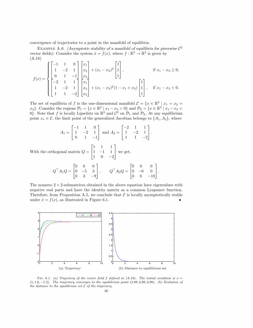
vector fields): Consider the system x = f(x), where f : R3 → R3 is given by(A.18)

f(x) =

−1 1 0

1 −2 1

0 1 −1

x1

x2

x3

+ (x1 − x3)2

1

1

1

, if x1 − x3 ≥ 0,

−2 1 1

1 −2 1

1 1 −2

x1

x2

x3

+ (x1 − x3)2(1− x1 + x3)

1

1

1

, if x1 − x3 < 0.

The set of equilibria of f is the one-dimensional manifold E = x ∈ R3 | x1 = x2 =x3. Consider the regions D1 = x ∈ R2 | x1−x3 > 0 and D2 = x ∈ R2 | x1−x3 <0. Note that f is locally Lipschitz on R3 and C2 on D1 and D2. At any equilibriumpoint x∗ ∈ E , the limit point of the generalized Jacobian belongs to A1, A2, where

A1 =

−1 1 01 −2 10 1 −1

and A2 =

−2 1 11 −2 11 1 −2

.

With the orthogonal matrix Q =

1 1 11 −1 11 0 −2

we get,

Q>A1Q =

0 0 00 −5 30 3 −9

, Q>A2Q =

0 0 00 −6 00 0 −18

.The nonzero 2× 2-submatrices obtained in the above equation have eigenvalues withnegative real parts and have the identity matrix as a common Lyapunov function.Therefore, from Proposition A.5, we conclude that E is locally asymptotically stableunder x = f(x), as illustrated in Figure 6.1. •

0 2 4 6 8 10−2

−1

0

1

2

3

4

x1 x2 x3

(a) Trajectory

0 2 4 6 8 100

0.5

1

1.5

2

2.5

3

3.5

4

4.5

(b) Distance to equilibrium set

Fig. 6.1. (a) Trajectory of the vector field f defined in (A.18). The initial condition is x =(1, 1.6,−1.2). The trajectory converges to the equilibrium point (2.88, 2.88, 2.88). (b) Evolution ofthe distance to the equilibrium set E of the trajectory.

26