June 2014

Sacramento Municipal Utility District High Penetration Photovoltaic Initiative

URS CORPORATION

HIGH PENETRATION PHOTOVOLTAIC INITIATIVE

Renewable Energy Technical Services 4500068205, Task Order 06

Final June 2014

Sacramento Municipal Utility District 6201 S Street

Sacramento, CA 95852-1830

Prepared by

2870 Gateway Oaks Drive, Suite 150

Sacramento, CA 95833

STATEMENT OF LIMITATIONS

This document is a compilation of documents provided to URS by SMUD. URS has relied on the information in these documents as furnished, and is neither responsible for nor has confirmed the accuracy of the information.  

Contents

Abstract

Executive Summary

1.0 Introduction ...................................................................................................................... 1-1

1.1 HIP-PV Initiative Tasks ............................................................................................. 1-1

1.2 About the Team ....................................................................................................... 1-1

1.2.1 SMUD ........................................................................................................... 1-1

1.2.2 Hawaiian Electric .......................................................................................... 1-1

1.2.3 DNV KEMA Energy & Sustainability ............................................................. 1-2

1.2.4 NEO Virtus Engineering, Inc. ........................................................................ 1-2

1.2.5 Electric Power Research Institute ................................................................ 1-2

2.0 Project Overview and Goals .............................................................................................. 2-1

2.1 Overview ................................................................................................................. 2-1

2.2 Goals ........................................................................................................................ 2-2

3.0 System Modeling, Field Monitoring and Analysis ............................................................. 3-1

3.1 Objectives ................................................................................................................ 3-1

3.2 Approach ................................................................................................................. 3-2

3.2.1 Baseline Modeling of Feeders for SMUD, HECO, HELCO, and MECO .......... 3-2

3.2.2 Hawaii Solar Irradiance Data Analysis .......................................................... 3-4

3.3 Findings ................................................................................................................... 3-8

3.3.1 SMUD Substation and Feeder Analysis ........................................................ 3-8

3.3.2 HECO Substation and Feeder Analyses ...................................................... 3-23

3.4 Conclusion ............................................................................................................. 3-33

4.0 PV Inverter Communications ............................................................................................ 4-1

4.1 Objectives ................................................................................................................ 4-1

4.2 Approach ................................................................................................................. 4-2

4.2.1 Test Architecture ......................................................................................... 4-2

4.2.2 Inverter Communications ............................................................................ 4-6

4.2.3 Test Equipment Arrangement ..................................................................... 4-6

4.3 Findings ................................................................................................................... 4-9

4.3.1 No Significant Issues .................................................................................... 4-9

4.3.2 Implications for Widespread Deployment ................................................... 4-9

4.3.3 Findings and Other Considerations ........................................................... 4-12

i

5.0 System Integration and Visualization Tools ...................................................................... 5-1

5.1 Objectives ................................................................................................................ 5-1

5.2 Approach ................................................................................................................. 5-3

5.2.1 Renewable Data Architecture and Analytics ............................................... 5-8

5.2.2 Locational Value Maps ............................................................................... 5-13

5.2.3 REWatch ..................................................................................................... 5-17

5.2.4 Operations Integration .............................................................................. 5-18

5.3 Outcomes .............................................................................................................. 5-22

5.4 Lessons Learned .................................................................................................... 5-22

6.0 Solar Monitoring and PV Production Forecasting ............................................................. 6-1

6.1 Objectives ................................................................................................................ 6-1

6.2 Approach ................................................................................................................. 6-2

6.2.1 Design, Manufacture, Deploy and Maintain 5 km Irradiance Monitoring Network .................................................................................... 6-2

6.2.2 Develop 20-36 Hour Feed-Forward PV Forecasting Model ....................... 6-13

6.2.3 Develop 0-3 Hour Feed-Forward PV Forecasting Model ........................... 6-19

6.2.4 Validate Irradiance/PV Production/Load Forecast Models ....................... 6-22

6.3 Production Forecasting Outcomes ........................................................................ 6-31

6.3.1 5 km Grid Irradiance Network (NEO and SMUD) ....................................... 6-31

6.3.2 Forecast PV Production Piece-wise Program (NEO and Contractors) ....... 6-31

6.3.3 One Year Measured 5 km, 1 Min Rate, Irradiance and Ambient Temp Data (NEO and Contractors) ...................................................................... 6-31

6.3.4 One Year Day-ahead Forecast PV Production Data by Site, 1 Hour Intervals (NEO and Contractors) ................................................................ 6-32

6.3.5 One Year 3-hour Forecast PV Production Data by Site, 15 Min Intervals (NEO and Contractors) ................................................................ 6-32

6.4 Production Forecasting Lessons Learned .............................................................. 6-33

7.0 Lessons Learned ................................................................................................................ 7-1

8.0 General Conclusions .......................................................................................................... 8-1

ii

Prior Reports

1. High Penetration PV Initiative: Case Descriptions

2. High Penetration PV Initiative: Monitoring Deployment

3. Report on Base Line Modeling on Sacramento Municipal Utilities District and Hawaiian Electric Companies Systems

4. High Penetration PV Project (Hi-PV) Report on Impacts to Transmission and Distribution Grids

5. Smart Inverter Advanced Metering Infrastructure Integration Using Smart Energy Profile

6. HIP-PV Task 4: Visualization of High Penetration PV, Final Report

7. High Penetration PV Initiative: PV Monitoring and Production Forecasting

iii

Tables

Table 3-1. Feeders selected for analysis ................................................................................. 3-3 Table 3-2. Summary of results for Substation CT ................................................................. 3-13 Table 3-3. Summary of reverse power flow and voltage changes ....................................... 3-15 Table 3-4. Summary of L7 simulation results ....................................................................... 3-22 Table 3-5. MI feeders SLACA, existing and planned PV penetration by feeder and

cluster .................................................................................................................. 3-24 Table 3-6. Estimate of portion of feeders trunk with reverse current flow for WA

analysis ................................................................................................................ 3-30 Table 3-7. kW installed kva installed on WO 3 ..................................................................... 3-32 Table 3-8. Study summary .................................................................................................... 3-36 Table 4-1. Equipment list ........................................................................................................ 4-4 Table 5-1. List of monitoring devices, communication, and data resolution ......................... 5-7 Table 5-2. Targeted visualization capabilities ........................................................................ 5-8 Table 6-1. Irradiance and PV production forecast error comparison for day-ahead

forecasts .............................................................................................................. 6-23 Table 6-2. Day-ahead irradiance, PV, and 0-3 hour PV production forecast error

comparison .......................................................................................................... 6-29 Table 6-3. NEO NDFD day-ahead forecasts compared to a persistence model ................... 6-31

Figures

Figure 3-1. MECO irradiance full week, three time increments .............................................. 3-6 Figure 3-2. MECO irradiance select day, three time increments ............................................. 3-7 Figure 3-3. EG feeder diagram ................................................................................................. 3-8 Figure 3-4. July 2012 load curve for EG ................................................................................... 3-9 Figure 3-5. EB feeder with PV plant, digester and cogeneration plant ................................. 3-11 Figure 3-6. CT feeder diagram ............................................................................................... 3-12 Figure 3-7. Feeder layout for AC1, AC2, and AC3 (AC1 in blue, AC2 in green, and AC3

in red) .................................................................................................................. 3-14 Figure 3-8. AC1 power flows for minimum daytime peak conditions ................................... 3-14 Figure 3-9. Voltage profile for all cases ................................................................................. 3-16 Figure 3-10. AC1, AC2, and AC3 power flow and voltage profiles for Scenario 2A ................. 3-17 Figure 3-11. AC2 feeder SynerGEE model ............................................................................... 3-19 Figure 3-12. AC2 Smart Home community .............................................................................. 3-19 Figure 3-13. L7 feeder one-line diagram ................................................................................. 3-21 Figure 3-14. RF one-line diagram ............................................................................................. 3-22 Figure 3-15. SynerGEE illustration of the geographical and electrical focal areas for

MI cluster ............................................................................................................. 3-24 Figure 3-16. Penetration percentage for technical criteria violation on feeder,

transformers, or cluster ....................................................................................... 3-25 Figure 3-17. Combined penetration limits graph for MI feeders, transformers, and

cluster .................................................................................................................. 3-26 Figure 3-18. ML SynerGEE model ............................................................................................ 3-27 Figure 3-19. ML12 (top) and 14 (bottom) transformer tap position vs. PV penetration % ..... 3-28 Figure 3-20. SynerGEE electric model of WA substation ......................................................... 3-29

iv

Figure 3-21. WO 3 geography of PV locations ......................................................................... 3-30 Figure 3-22. WO feeders load, maximum left-hand side and minimum right-hand side ........ 3-31 Figure 3-23. WO 3 backfeed analysis for three loading conditions ......................................... 3-31 Figure 3-24. Maximum % fault current increase for WO 3 ...................................................... 3-32 Figure 4-1. Testing at SMUD facility ........................................................................................ 4-3 Figure 4-2. Testing at EPRI Knoxville Laboratory ..................................................................... 4-3 Figure 4-3. Power wiring diagram ............................................................................................ 4-7 Figure 4-4. Inverter and DC power supply ............................................................................... 4-7 Figure 4-5. Inverter with power and communication connections ......................................... 4-8 Figure 5-1. System uncontrolled ramp concerns due to solar (source: HELCO) ...................... 5-3 Figure 5-2. Observed increase in local feeder LTC movement due to solar

(source: HECO) ....................................................................................................... 5-4 Figure 5-3. Examples of solar monitoring devices deployed in Hawaii and California ............ 5-4 Figure 5-4. Remote wind monitoring sensors (SODAR and LIDAR) and temperature

profilers (radiometer) deployed in Hawaii as part of the forecasting network (WindNET) ............................................................................................... 5-5

Figure 5-5. Architecture for data management and exchange using T-REX ............................ 5-9 Figure 5-6. Perspective view of renewable data and customizable data-handling

features (A-D) ...................................................................................................... 5-10 Figure 5-7. Analysis of solar data on Oahu using the Perspective interface to T-REX

(source: HECO) ..................................................................................................... 5-11 Figure 5-8. (a) Visual confirmation of mid-day (10 a.m. to 2 p.m. for Hawaii) impact of

PV on different types of feeder loads (commercial, residential, industrial or combined) at different resolutions with different monitoring devices (SCADA and Basic Measuring Instrument power monitoring devices) and (b) measured backfeed condition (source: HECO) .............................................. 5-12

Figure 5-9. Online LVM front page ........................................................................................ 5-14 Figure 5-10. Sample online address query display results ...................................................... 5-15 Figure 5-11. New 5-tone LVM with (a) percentage penetration of circuit maximum,

(b) percentage penetration by circuit daytime minimum load and (c) all island summary (source: HECO) ................................................................. 5-17

Figure 5-12. Renewable Watch for Oahu ................................................................................ 5-18 Figure 5-13. Conceptual view of new data and EMS environment enhancements ................ 5-19 Figure 5-14. Prototype of regional forecasts and ramp statistics (source: Siemens and

HECO) ................................................................................................................... 5-21 Figure 6-1. Primary station (rotating shadowband radiometer) located on roof of

California State University Sacramento ................................................................. 6-3 Figure 6-2. Fabrication of the secondary stations at NEO Virtus Engineering, Inc. ................. 6-4 Figure 6-3. SMUD lineman installing one of the secondary stations in Sacramento,

California ................................................................................................................ 6-5 Figure 6-4. SMUD-NEO irradiance network ............................................................................. 6-6 Figure 6-5. Loggernet RTMC data monitoring window; secondary sensors 12 to 22 ............. 6-7 Figure 6-6. Battery state of charge view screen; 66 stations .................................................. 6-8 Figure 6-7. Irradiance signals on 2 clear days, 2 weeks apart ................................................. 6-9 Figure 6-8. One of the four RSRs with a PSP installed ........................................................... 6-10 Figure 6-9. Locations of four Eppley Precision Spectral Pyranometers ................................. 6-11 Figure 6-10. NEO solar forecast graphical user interface ........................................................ 6-12

v

Figure 6-11. Sample from two sites, comparing forecast and measured production on mostly clear days ............................................................................................ 6-18

Figure 6-12. Example of initial methodology for 0-3 hour irradiance forecast: Ground Level Irradiance Velocity Vector Recognition ...................................................... 6-20

Figure 6-13. Diagram of neural-network applied in the prediction......................................... 6-21 Figure 6-14. Output from neural net 0-3 hour GHI forecast compared with measured

GHI on a clear day ................................................................................................ 6-21 Figure 6-15. Output from neural net 0-3 hour GHI forecast compared with measured

GHI on a cloudy day ............................................................................................. 6-22 Figure 6-16. Kammerer forecast vs. measured power, Oct 1 – 7, 2012 .................................. 6-24 Figure 6-17. Measured vs. forecast irradiance for Sensor 10 (closest to Kammerer),

Oct 1 – 7, 2012 ..................................................................................................... 6-24 Figure 6-18. Average monthly measured power per FIT site .................................................. 6-25 Figure 6-19. Metric monthly variation ..................................................................................... 6-26 Figure 6-20. Scatter plot of hourly measured vs. 20-36 hour forecast PV power for the

four fixed array FIT sites ...................................................................................... 6-27 Figure 6-21. Scatter plot of hourly measured vs. 20-36 hour forecast power for the

three tracking FIT sites ........................................................................................ 6-28

vi

Acronyms and Abbreviations

Item Description

AMI advanced metering infrastructure

ART Atmospheric Research and Technology

BEW BEW Engineering

BORCAL Broadband Outdoor Radiometer Calibration

CCD charge coupled device

CPUC California Public Utilities Commission

CSI RD&D California Solar Initiative Research, Development, Demonstration and Deployment

CSUS California State University Sacramento

DAQ data acquisition

DC direct current

DG distributed generation

DNI direct normal irradiance

DNV DNV KEMA Energy & Sustainability

DOE U.S. Department of Energy

DRLC demand response/load control

EMS energy management system

EPRI Electric Power Research Group

FastDR faster demand response

FIT feed in tariff

FSU field service unit

GHI global horizontal irradiance

GIS geographic information system

GPS global positioning system

GTI global tilted irradiance

HAN home area network

HECO Hawaiian Electric Company

HELCO Hawai`i Electric Light

HiP-PV High Penetration Photovoltaic Initiative

HRRR high resolution rapid refresh

IEEE Institute of Electrical and Electronics Engineers

IOU investor-owned utility

ISO Independent system operator

km kilometer

vii

Item Description

kV kilovolt

LIDAR light detection and ranging

LM locational monitors

Loggernet datalogger support software package by Campbell Scientific

LTC load tap changer

LVM locational value map

MAE mean absolute error

MECO Maui Electrical Company

MVA megavolt ampere

MVAr megavolt ampere reactive

MW megawatt

MySQL database for web-based applications

NDFD National Digital Forecast Database

NEO NEO Virtus Engineering, Inc.

NOAA National Oceanic and Atmospheric Administration

NREL National Renewable Energy Laboratory

PMI power quality monitors manufactured by Revolution

PSP Precision Spectral Pyranometers

PSS/E Power System Simulator for Engineering

PV photovoltaic

REST2 Reference Evaluation of Solar Transmittance 2 bands

RPS renewable portfolio standard

RSR rotating shadowband radiometer

RTMC real-time monitor and control

RTU remote terminal unit

SCADA supervisory control and data acquisition

SCS Solar Consulting Services

SEP Smart Energy Profile

SEPA Solar Electric Power Association

SLACA substation load and capacity analysis

SMS calibrated shadowband sensors for determining components of the total irradiance

SMUD Sacramento Municipal Utility District

SNI SMUD-NEO Irradiance Network

SODAR sonic detection and ranging

viii

Item Description

SSN Silver Spring Networks

SynerGEE electric distribution simulation model developed by GL Group

TJD reference irradiance sensors serving to join data to transmission infrastructure

UFLS under frequency load shed

V volts

VAC volts, alternating current

W watts

W/m2 watts per square meter

WAP wireless access point

Wh total watt-hours

WSU Wichita State University

ix

ABSTRACT

The lack of high quality, high resolution, field-measured photovoltaic (PV) data to inform modeling of high-penetration PV on the electrical system is a prevailing integration barrier, not only for the solar community but also for wind, storage, and other renewable development activities. To help fill this void, Sacramento Municipal Utility District (SMUD) and Hawaiian Electric Company (HECO) collaborated on the High Penetration PV (HiP-PV) Initiative to develop distributed PV visualization tools supported by ongoing field monitoring and data analysis at sites of interest, including the development and testing of hardware and software to support the project. This work was done under a California Public Utilities Commission and California Solar Initiative Research, Development, Demonstration and Deployment HIP-PV Initiative Grant Program.

Circuits throughout California and Hawaii already experience high levels of PV penetration with more on the near horizon, so the HiP-PV Initiative used case studies in these areas for field monitoring, data collection and analysis, system modeling and simulation, and software and hardware development and testing. The sites focused on cases of existing high penetrations or potential for high penetrations of PV, each requiring different levels of monitoring and related effort. These case studies provided the data necessary for developing and integrating the HiP-PV visualization tools (planning, operational, and forecasting) to assist SMUD and HECO in identifying optimal locations that can accommodate more distributed resources (e.g., PV) and to visually track and trend changes within their respective distribution systems. The HiP-PV tools and research will be useful to other utilities to plan and improve their distribution systems.

Abstract – 1

EXECUTIVE SUMMARY

The Sacramento Municipal Utility District (SMUD), in partnership with the Hawaiian Electric Company (HECO), conducted a research, demonstration, and deployment project that targeted testing and development of hardware and software for high penetration photovoltaic (PV). This project, known as the High Penetration PV (HiP-PV) Initiative was intended to address key grid integration and operational barriers that hinder larger-scale PV adoption into mainstream operations and onto the distribution grid. Both utilities are currently managing the introduction of high penetration PV into their systems. As part of the HiP-PV Initiative, SMUD and HECO identified case study locations in California and Hawaii, solar assessment and forecasting needs, and PV grid integration and visualization needs. This work was done under a California Public Utilities Commission (CPUC) and California Solar Initiative Research, Development, Demonstration and Deployment (CSI RD&D) HIP-PV Initiative Grant Program.

The HiP-PV activities addressed key integration barriers in visualizing, monitoring, and controlling high-penetration PV on the grid. Specific activities included:

• Development of a software visualization tool to enable identification of high value locations for distributed PV on the distribution system and to identify problem areas that will require reinforcement or modification to enable high penetrations. Smart siting of renewable distributed generation involves fully understanding the solar resource, its potential deployment, and interaction with the existing distribution infrastructure. Case studies include residential, commercial, and greenfield sites overlaid throughout the electrical system in order to assess interconnection benefits (cost and locational value) to the system.

• Development of a renewable generation operational tool that allows utilities to see how the renewable generation is functioning on their systems. This tool enables full use of distributed PV in displacing the need for distribution upgrades and natural gas peakers. It allowed validation of forecasting software, providing three hour-ahead and day-ahead PV output forecasts.

• Deployment of a solar irradiance sensor network and coordinated advance communication for controls (i.e., dedicated cellular, advanced metering infrastructure (AMI) network, supervisory control and data acquisition (SCADA) system-enabled condition monitoring, and distribution remote terminal units [RTUs]).

Summary of Outcomes

The production of this High Penetration PV Initiative study summary represents major efforts by SMUD and the Hawaiian electrical utilities to understand the impacts of solar power generation on their distribution systems. The utilities are responding to an entirely new paradigm of distributed renewable power generation, which is often sporadic and difficult to predict. The utilities are using the latest smart grid technologies to monitor, simulate, and forecast impacts

Executive Summary – 1

on the distribution systems. What we see in these studies is the incremental development of smart grid devices and methodologies, which is to date an incomplete process.

The tools necessary for complete understanding of distribution system impacts are not completely evolved at this stage, but the tools and techniques are becoming more useful and available. Monitoring points are not standard and often they are inadequate to provide the data necessary for optimal system operation and planning. The simulation software is useful and has some degree of accuracy, but significant improvements are still needed. Forecasting of PV generation is still very dependent on accurate incoming data, but the data available may be insufficient and incomplete, and data collection systems need greater reliability. The variability of the weather, especially cloud cover in certain regions of Hawaii, appears to be a significant challenge even over small geographic areas.

The general conclusion is that utilities are making greater use of smart grid monitoring devices to assist with PV generation planning, operation, and forecasting. The systems to date are often still in the experimental stages in several aspects, but are improving with each application and effort to further understand the impacts of high penetration solar PV.

This study also points to a more global need for improvements to power distribution system equipment. In particular, equipment to help control load and voltage will go a long way toward improving distribution operations. Energy storage, more rapid response of voltage control devices, and integration of solar inverter control systems into distribution system control will allow greater PV penetration and will provide utilities with improved operational control.

Executive Summary – 2

1.0 INTRODUCTION

As utilities move towards a smart grid, becoming smarter about the siting of renewable distributed generation to maximize its benefit will help accomplish the combination of economic, reliability, and environmental goals that drive the utilities of today.

SMUD, in partnership with HECO, conducted the HiP-PV Initiative to address key grid integration and operational barriers that hinder larger-scale PV adoption into mainstream operations and onto the distribution grid. As two utilities managing grid integration of high-penetration PV, SMUD and HECO are coordinating research efforts at locations in California and Hawaii that served as case studies for assessing solar forecasting needs and PV grid integration and visualization tools. This project received funding from the CSI RD&D Program’s first grant solicitation. The CSI RD&D Program is administered by Itron, on behalf of the CPUC.

1.1 HIP-PV Initiative Tasks

The scope of this work was divided into the following five tasks:

• Task 1: Project Management, Technology Transfer, and Outreach (SMUD)

• Task 2: Baseline Modeling of SMUD and HECO Systems (DNV KEMA Energy & Sustainability [DNV], SMUD, and HECO)

• Task 3: Field Monitoring and Analysis (DNV, SMUD, and HECO)

• Task 4: System Integration and Visualization Tools Development (HECO)

• Task 5: Solar Resource Data Collection and Forecasting (NEO Virtus Engineering, Inc. [NEO Virtus] and SMUD)

1.2 About the Team

1.2.1 SMUD

SMUD is a publicly owned municipal electric utility (sixth largest in United States) with a service area of 900 square miles, serving 1.4 million (Sacramento County and parts of Placer County). SMUD serves nearly 600,000 residential, commercial, and industrial customers.

1.2.2 Hawaiian Electric

The Hawaiian Electric Companies are comprised of three sister electric utilities. Hawaiian Electric Company (HECO) provides electric services on the island of Oahu, Maui Electric Company (MECO) services the islands of Maui, Molokai and Lanai and Hawaii Electric Light Company (HELCO) serves the largest island of Hawaii. Together these utilities serve 95% of the Hawaii’s 1.2 million residents in the state of Hawaii.

Final – 1-1

1.2.3 DNV KEMA Energy & Sustainability

DNV provides classification and technical assurance along with software and independent expert advisory services to the maritime, oil and gas, and energy industries. They also provide certification services to customers across a wide range of industries. In 2013, DNV merged with GL, now operating in more than 100 countries with 16,000 professionals.

1.2.4 NEO Virtus Engineering, Inc.

NEO Virtus Engineering, Inc., is an electrical and solar engineering consulting firm specializing in photovoltaic electrical system design. They have served the technical needs of utilities, architects, Mechanical, Electrical, and Plumbing (MEP) engineering and architectural firms, environmental consulting firms, construction companies, and product developers/ manufacturers since 2001.

1.2.5 Electric Power Research Institute

Electric Power Research Institute (EPRI) is a nonprofit organization funded by the electric utility industry. It conducts research on issues related to the electric power industry in US. EPRI's area covers different aspects of electric power generation, delivery, and its use.

Final – 1-2

2.0 PROJECT OVERVIEW AND GOALS

2.1 Overview

SMUD and HECO partnered on this project because both utilities share synergistic problems on their distribution systems based on high penetration and the exponential growth of distributed generation (DG) PV deployment to meet renewable portfolio standard (RPS) and energy efficiency targets. California and Hawaii both have aggressive RPS and solar/DG goals (in California, 3,000 megawatts [MW] of solar PV, in Hawaii 4,300 gigawatt hours of distributed resources for energy efficiency) (California SB1 Million Solar Roofs Initiative, 2010). SMUD and HECO also share common issues:

• Lack of visibility on the system down to the distribution level

• Lack of reliable forecasting capability for solar and DG resources for effective operations especially during variable weather days and peak loads

In addition, SMUD and HECO share similar planning and operations tools for control of DG systems. Both systems have high penetration of variable renewable generation. Hawaii is already seeing a high penetration level of DG on the system, where as many mainland grids are just now concerned about potential impacts.

In both the California Intermittency Analysis and Hawaii’s past Clean Energy Initiative renewable integration efforts, there is a lack of high quality, high resolution, field-measured PV data to inform adequate modeling of high-penetration PV on the electrical system (CEC-500-2007-081, July 2007; Hawaii Clean Energy Initiative, 2008). This condition is a prevailing integration barrier not only for the solar community but also for wind, storage, and other renewable development activities. Envisioned as part of this effort, SMUD and HECO collaborated in developing the HiP-PV Initiative focused on development of distributed PV visualization tools supported by on-going field monitoring and data analysis at sites of interest; development and testing of hardware and software for enabling HiP-PV; and transfer of lessons learned.

As distributed PV and large-scale PV facilities continue to be planned and developed in both states, there is a need to implement quality field measurement campaigns and amass accurate data for improving electrical system models to include PV generators and integration control characteristics. Information developed can help inform PV manufacturers’ development of new software, hardware, and communications approaches to respond to these needs.

With circuits throughout both California and Hawaii already experiencing high levels of PV penetration, and more on the near horizon, SMUD and HECO were able to identify immediate case studies for field monitoring, data collection and analysis, system modeling and simulation, and software and hardware development and testing. The studies focused on cases of immediate interest (e.g., existing high penetrations or potential for high penetrations of PV), each requiring different levels of monitoring and effort.

Final – 2-1

The HiP-PV Initiative is organized into five tasks:

1. Project Management, Technology Transfer, and Outreach

2. System Modeling

3. Field Monitoring and Analysis

4. System Integration and Visualization Tools Development

5. PV Production Forecasting

These case studies provided the necessary data and modeling for development and integration of the inverter communications equipment, HiP-PV visualization tools (planning, operational, and forecasting), modeling tools, and monitoring and production forecasting techniques to assist SMUD and HECO in evaluating locations that can reliably benefit from and accommodate more PV distributed resources. Both utilities continue to visually track and trend changes within their respective distribution systems using lessons learned from these initial sites.

2.2 Goals

Integrating high penetrations of solar PV requires substantial changes in the way today’s electricity grid is designed and operated. It requires new tools for understanding PV as a distributed generation resource, new hardware and software for communicating with and controlling thousands of generation sources, and modifications to the top-down electricity grid to enable bi-directional flow management throughout the grid. Current tools and understanding of PV are acceptable in a world where PV provides less than 1% of total capacity, but adoption rates in PV technology and state RPS goals indicate this paradigm will not last. Thus utilities must adopt new hardware and software and reconfigure and facilitate operational changes today to ensure a smooth transition to higher PV penetration grid scenarios. The HiP-PV activities addressed key integration barriers in visualizing, monitoring, and controlling high penetration PV on the grid.

To attain future smart grid and clean energy targets for the respective utility operating environments, a goal for both SMUD and Hawaii utilities is the development of a sustainable portfolio of energy supply (existing generation) and energy load management capabilities, including distributed generation, customer load management, and other demand side management programs. An advanced vision and enabling control technologies, akin to the Solar Energy Grid Integration Systems concept (Sandia National Laboratories: Solar Energy Grid Integration Systems–Energy and Climate, November 29, 1012), are therefore needed for transforming the existing, relatively small PV energy market comprised of passively interacting systems to a high-penetration active partner providing support services to the overall grid. Such a system necessarily requires a strong understanding of solar resources and potential, tools to identify optimal siting locations and problem areas, predictive output tools, and strong communications and control approaches.

Final – 2-2

SMUD and HECO expect over the next several years that the penetrations of PV will reach levels requiring significant mitigation measures on the distribution system to maintain reliability, voltage control, and fault identification capabilities. An over-arching objective of this work is to identify practical mitigation strategies for managing high penetrations of PV, which not only allows PV to reach higher penetrations, but ensure that it does so in a way that enhances grid reliability in the face of economic and environmental constraints. Meeting minute to minute demand with distributed intermittent resources providing a significant amount of the energy is a challenge. Doing it with a minimal amount of costly energy storage requires smart planning, much greater understanding of the solar resource, and a fundamental change in the communications and controls systems grid operators currently use to interact with generation resources. The HiP-PV Initiative addresses each of these areas to support HECO’s and SMUD’s goal of demonstrating successful integration of very high penetrations of solar PV.

The HiP-PV Initiative activities address key integration barriers in visualizing, monitoring, and controlling high penetration PV on the grid, including:

• Development of a software visualization tool to enable identification of high value locations for distributed PV on the distribution system and to identify problem areas that will require reinforcement or modification to enable higher penetrations of PV.

• Development of a renewable generation operational tool that allows utilities to see how the renewable generation is functioning on their systems.

• Deployment of a solar irradiance sensor network and coordinated advance communication for controls.

Final – 2-3

3.0 SYSTEM MODELING, FIELD MONITORING AND ANALYSIS

Note: Information in this section is excerpted from High Penetration PV Initiative: Case Descriptions; High Penetration PV Initiative: Monitoring Deployment; Report on Base Line Modeling on Sacramento Municipal Utilities District and Hawaiian Electric Companies Systems, and High Penetration PV Project (Hi-PV) Report on Impacts to Transmission and Distribution Grids. 1

This component of the project studies the potential impact of high penetration of PV resources on distribution circuits on the SMUD and HECO grids.

3.1 Objectives

The distribution database includes details from the substation to the end-use load and also the PV and inverter characteristics. The distribution circuit model is intended to leverage the existing distribution modeling work, with HECO using a model developed with SynerGEE (electric distribution simulation model developed by DNV GL (formerly BEW)) at the 46 kilovolt (kV) and 12 kV levels. SMUD provided the distribution circuit models for DNV GL to use in this study. DNV GL and SMUD worked together in reviewing the modeling detail of specific circuit feeders.

Adequate modeling of the distribution circuits is an essential first step of the work needed to investigate impacts on grid operation with an increasing content of variable renewable energy and to help develop control and mitigation strategies. The modeling should attempt to address how to account for PV variability and what role the software distribution models should have in addressing this complex issue. The specific objectives are as follows:

• Identify high penetration analysis needs (load flow, characteristics of the load, protection/coordination, voltage regulation, and islanding) for the distribution circuit being analyzed.

• Identify additional data parameters to be collected and locations along the high penetration distribution circuit to place additional high-fidelity monitoring equipment, as necessary.

• Record and collect at a minimum 6 to 12 months’ worth of high-fidelity load data from the newly installed high-fidelity monitoring equipment.

• Collect electrical equipment nameplate data from the distribution system being analyzed: distributed generation on the circuit, inverters, any energy storage, circuit size, circuit length, circuit loading, switchgear, and transformers to be used in the model development.

• Investigate varying incremental levels of PV penetration at the distribution capacity level and iterate with an existing system level model to understand to what degree higher PV levels will adversely affect the grids.

1 TBD – Final DNV GL report

Final – 3-1

• Based on the validation results for a single circuit study, develop a methodology for extending the findings using the simulation tools to inform and expedite interconnections studies at higher penetration levels.

The first task was the development and validation of SynerGEE data sets for the feeders selected by SMUD and HECO. The data sets were used to simulate different aspects of SMUD’s and HECO’s power systems including electrical characteristics of the distribution circuit and relevant characteristics of PV inverters. The tasks provided a validation analysis of the model performance. Validation was performed over several analytical time frames. Through data collection, modeling, and analysis, the detailed single circuit study will help identify barriers (data gaps, as-built infrastructure limit) and inform system-level considerations and potential strategies for accommodating higher PV penetration levels. Part of the evaluation and validation study included circuit voltage profiles and impacts, voltage regulation, voltage flicker, islanding, fault conditions, and thermal limitation.

3.2 Approach

3.2.1 Baseline Modeling of Feeders for SMUD, HECO, HELCO, and MECO

Historically, electric utility distribution planners were not too concerned about installing power quality meters, solar sensors, and solar monitors on the distribution feeders. There was not an urgent need to validate voltages, frequency, and backfeed on the feeders since the power flows were from the distribution substation to the end of the feeder. Distribution feeders are normally radial lines, so as long as the voltage at the end of the line was within voltage tolerances, everything was fine. Sometimes a customer installed a cogeneration plant to self-generate but not to export to the utility.

Distribution planners normally set the voltage regulation point at the distribution substation bus between 122 and 125 volts so that the end of the feeder had a voltage ranging from 115 to 122 volts. If the voltage dropped too low toward the end of the feeder, the planner installed capacitor banks or regulators, depending on the length of the feeder. If multiple feeders were served from the same substation bus, the transformer tap changer was set to a regulation point that provides the same voltage on all the feeders

Distributed demand-side resources and new technologies have changed the distribution planning process and operational control of the transmission/distribution grids. Availability of low-cost roof-mounted solar panels, subsidies from state and local agencies, emission reduction requirements, and RPS requirements are rapidly increasing the penetration of distribution generation on the feeders. As these increase in magnitude, more voltage, frequency, power factor, reverse power flow, and protection issues must be addressed. Today, high PV generation and other demand-side technologies are not evenly distributed on all feeders or at the same locations on the feeder.

Final – 3-2

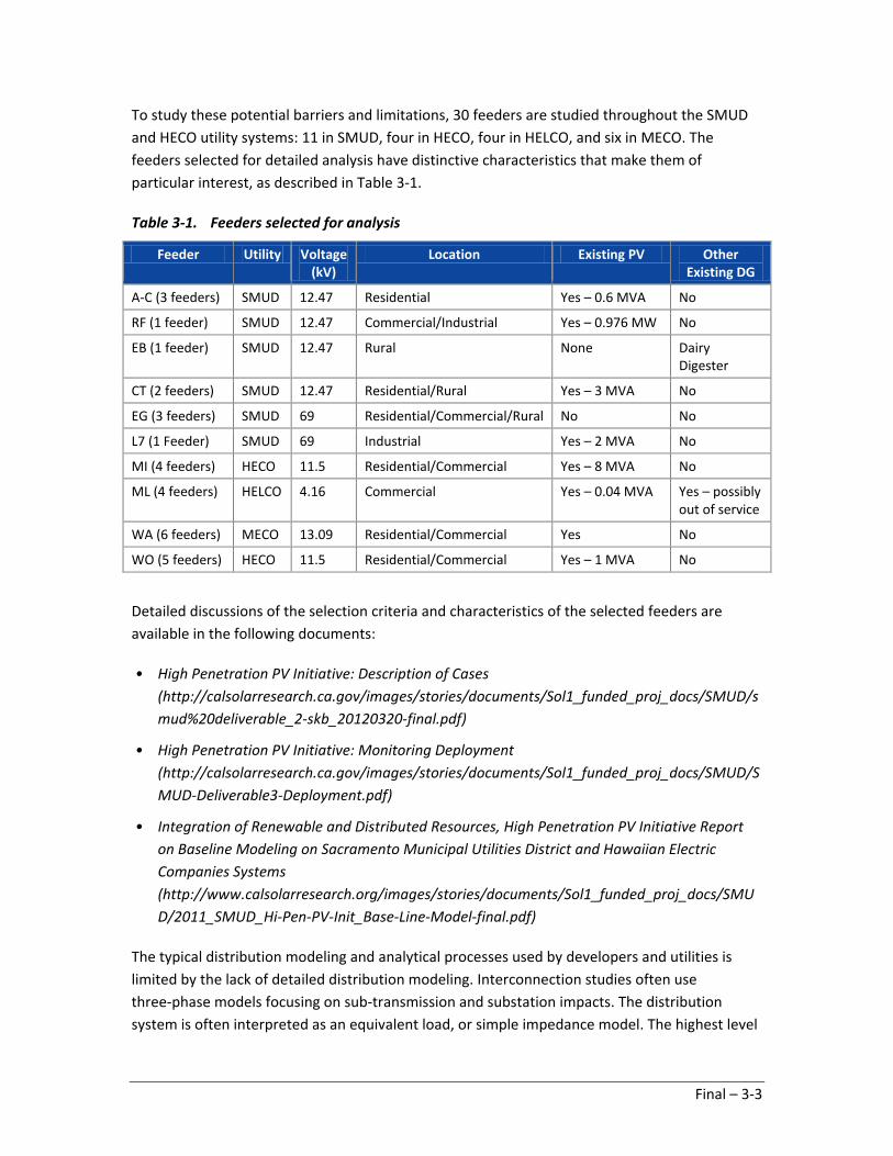
To study these potential barriers and limitations, 30 feeders are studied throughout the SMUD and HECO utility systems: 11 in SMUD, four in HECO, four in HELCO, and six in MECO. The feeders selected for detailed analysis have distinctive characteristics that make them of particular interest, as described in Table 3-1.

Table 3-1. Feeders selected for analysis

Feeder Utility Voltage (kV)

Location Existing PV Other Existing DG

A-C (3 feeders) SMUD 12.47 Residential Yes – 0.6 MVA No

RF (1 feeder) SMUD 12.47 Commercial/Industrial Yes – 0.976 MW No

EB (1 feeder) SMUD 12.47 Rural None Dairy Digester

CT (2 feeders) SMUD 12.47 Residential/Rural Yes – 3 MVA No

EG (3 feeders) SMUD 69 Residential/Commercial/Rural No No

L7 (1 Feeder) SMUD 69 Industrial Yes – 2 MVA No

MI (4 feeders) HECO 11.5 Residential/Commercial Yes – 8 MVA No

ML (4 feeders) HELCO 4.16 Commercial Yes – 0.04 MVA Yes – possibly out of service

WA (6 feeders) MECO 13.09 Residential/Commercial Yes No

WO (5 feeders) HECO 11.5 Residential/Commercial Yes – 1 MVA No

Detailed discussions of the selection criteria and characteristics of the selected feeders are available in the following documents:

• High Penetration PV Initiative: Description of Cases (http://calsolarresearch.ca.gov/images/stories/documents/Sol1_funded_proj_docs/SMUD/smud%20deliverable_2-skb_20120320-final.pdf)

• High Penetration PV Initiative: Monitoring Deployment (http://calsolarresearch.ca.gov/images/stories/documents/Sol1_funded_proj_docs/SMUD/SMUD-Deliverable3-Deployment.pdf)

• Integration of Renewable and Distributed Resources, High Penetration PV Initiative Report on Baseline Modeling on Sacramento Municipal Utilities District and Hawaiian Electric Companies Systems (http://www.calsolarresearch.org/images/stories/documents/Sol1_funded_proj_docs/SMUD/2011_SMUD_Hi-Pen-PV-Init_Base-Line-Model-final.pdf)

The typical distribution modeling and analytical processes used by developers and utilities is limited by the lack of detailed distribution modeling. Interconnection studies often use three-phase models focusing on sub-transmission and substation impacts. The distribution system is often interpreted as an equivalent load, or simple impedance model. The highest level

Final – 3-3

of existing detail is normally a three-phase aggregated load flow model. Most impact studies consider capacity and baseline generation. Impact of variable high PV penetrations is not generally quantified, due to a lack of accurately measured irradiance data for the PV.

An enhanced distribution modeling and analysis process was developed and compared to the simplistic process to determine the level of detail required in future studies. This project accurately quantifies the effect of high penetrations of PV on the distribution and sub-transmission systems. The modeling detail includes detailed inverter and PV modeling and performance.

The analysis determines the effect of variable resources and associated weather conditions on the distribution grid as a whole. The following steps developed the feeder data set for analysis:

• Extract geographic information system (GIS) or build (when GIS not available) SynerGEE model (although this study was done in SynerGEE, other equivalent simulation tools could be used)

• Collect and apply detailed equipment information

– Transformers, switches, fuses, capacitors, inverters, PV panels, etc.

• Collect PV data for area of interest, if available

• Analyze PV performance

– Associated weather data

• Model inverters

– Future detailed SynerGEE model, or

– Existing equivalent impedance model, and

– Power System Simulator for Engineering (PSS/E) dynamic inverter model, when applicable

Baseline modeling for the selected feeders includes data collection, evaluation, modeling, and analysis of the existing system with available data. PV data and representative load profiles are monitored for SMUD and the Hawaiian utilities. As more data are collected and evaluated, more analysis on the feeders of interest is completed.

3.2.2 Hawaii Solar Irradiance Data Analysis

Background. HECO, in partnership with the National Renewable Energy Laboratory (NREL), installed solar monitors and power quality meters in select locations across Oahu, Maui, the Big Island, Lanai, and Molokai to gather high fidelity irradiance and power monitor data. All of the Hawaii Solar Irradiance Data analyses are based on irradiance data with monitors on the substations. DNV KEMA Energy & Sustainability (DNV) obtained access to these data for the solar irradiance studies. The data were analyzed and input into distribution models to study the

Final – 3-4

impacts on high PV penetrations on the Hawaii distribution system. Work is continuing under a separate CSI RD&D grant. DNV is working with utility staff to gather feedback on the system conditions based on time stamped data and weather conditions and evaluating correlations between utility load, solar resources, and PV generation to develop a process of quantifying impacts due to common environmental conditions (e.g., cloudy, partially cloudy, clear sky) which can significantly impact solar sites.

Analysis. To accurately analyze solar irradiance data, high fidelity data are required. This section discusses an investigation into the value of high fidelity data. To accomplish this, direct comparisons are made between raw 1-minute irradiance data, 5-minute irradiance averages, and 1-hour irradiance averages. This aids in the determination of the acceptable time increment between data recordings for any particular type of analysis. For example, if calculating total annual irradiance, greater time increments between data points is acceptable. However, if analyzing aspects of the distribution systems, such as voltage flicker caused by PV variability, high fidelity data are necessary to inspect the immediate response in voltage data.

The 1-minute solar data (the highest level of data detail currently available through MECO from MECO Sub2 solar sensor) is chosen for this analysis. To compare the effects of average and reduced data fidelity, 5-minute and 1-hour time periods are also chosen for analysis. For this test, the raw data are averaged into 5-minute and 1-hour increments by simply adding the irradiance values and dividing by the number of recordings in that time (5 or 60). A number of time increment options are possible in further studies, such as snap shot readings instead of averages at any desired time interval.

The raw 1-minute irradiance data, 5-minute averages, and 1-hour averages are graphed in Figure 3-1 for the first week of July 2010. The data were originally recorded in coordinated universal time, so the data actually start at 2:00 p.m. June 30 until 2:00 p.m. July 7. The first bell curve of each graph occurs on July 1, 2010; the second bell curve occurs on July 2, 2010, etc. The three graphs are stacked vertically on top of each other in Figure 3-2 for direct comparison. One-minute data are on top, 5-minute average data are in the middle, and 1-hour average data are the bottom graph. Due to reduced number of data points in the 5-minute and 1-hour average graphs, a two-point moving average trend line is applied to the scatterplot data.

Final – 3-5

Figure 3-1. MECO irradiance full week, three time increments

Each day of sunlight hours in the 1-minute raw data graph contains roughly 740 data points, depending on the exact time of sunrise and sunset. Each day in the 5-minute averages graph contains roughly 148 data points, and each day in the 1-hour averages graphs contains only about 12 data points.

To demonstrate the issues with the potential averaging or miss application of data, closer inspection of one individual day, July 1, 2010, is shown in Figure 3-2. This day is selected for closer analysis because it exhibits the least amount of irradiance variability in the raw data of this week.

Final – 3-6

Figure 3-2. MECO irradiance select day, three time increments

Again, 1-minute raw irradiance data are the top graph in this figure, the five 5-minute average data are the middle graph, and the 1-hour average data are the bottom graph. Although the X axes do not have time labels for visual simplicity, the times quoted in the text are accurate and sourced from the data.

Even though July 1 is the least variable day of the week, there is still a drop in irradiance during the afternoon at 4:20 p.m. This is clearly apparent in the 1-minute raw data graph and appears quite significant, with initial magnitude loss of 500 watts per square meter (W/m2) and continued disruptions for about 1 hour and 45 minutes. This irradiance drop is still visible in the 5-minute averages graph, but with reduced severity. The magnitude of the irradiance drop in the 5-minute averages graph is reduced to 400 W/m2 with continued disruptions for only about an hour. In the final graph of 1-hour averages, no disruption is apparent. There is a very subtle dip in the trend line in last segment of line, but all detail is lost.

This smoothing caused by averaging data into larger time increments is a problem. It is clear that data fidelity is lost when using the 1-hour time step. If the 1-hour average graph of Figure 3-2 is

Final – 3-7

the only data available for this day, it appears to be a perfect clear sky day even though in reality this is not the case. This loss of accuracy may be acceptable for some applications, such as summing total monthly or annual irradiation; however, it is unacceptable for short- term applications. Very short time scales and high fidelity data are necessary to determine the exact effect of PV on the distribution system. Ramp rate analysis to define power stability, voltage fluctuations, etc., is not possible with data that have lost the necessary level of detail due to large time increments.

3.3 Findings

The following describes the feeders and the findings of the voltage load flow and system analyses with HiP-PV.

3.3.1 SMUD Substation and Feeder Analysis

3.3.1.1 EG Substation and 69 kV Line Analysis

EG Bank 1 consists of one 230/69 kV transformer with two 69 kV circuits (3 and 4). Sixteen 69/12 kV distribution transformers connected to the circuits that have 32 12 kV feeders. There are three major central PV plants connected to the 69 kV circuits with a total connected rating of 48 MW. Figure 3-3 displays the layout of the two 69 kV circuits. The sources of PV generation data are calculated from actual irradiance data near the site.

Figure 3-3. EG feeder diagram

Data are provided for July 2012 from which the peak hour is July 12, 2012, at 6 p.m. Figure 3-4 shows the 24 load profile and the corresponding solar generation for the day. The recorded demand data, including the PV generation, are considered the net load and shown as the red

Final – 3-8

line. The gross load or load without solar generation is the combination of the solar generation and net load as shown by the blue line. The individual solar generation profiles are shown at the bottom of the figure. One of the PV installations has a tracker system that extends the peak solar generation longer in the day.

Figure 3-4. July 2012 load curve for EG

The EG area is projected to have distributed solar generation and higher penetrations of central solar plants on the 69 kV circuits. The analysis completed for the peak day with increasing PV scenarios indicates that the system can experience reverse power flow, directional power flows even on the peak day, and potential voltage violations. This analysis suggests the need to conduct studies on other non-peak load days and even time sequential power flow modeling to determine the impacts on the 69 kV circuits, the 12 kV distribution circuits, and even perhaps the 230 kV grid.

A summary of this analysis of EG Bank 1 is as follows:

• EG Bank 1 2012 peak load ~137 MW on July 12 at 6 p.m.

• Three load flow scenarios explored with peak load: PV penetration level of 0% (no PV),15% (~20.5 MW), and 30% (~41 MW); PV added at the locations of existing generators

• Maximum % of a single 69 kV line loading for the three cases: 89%, 86%, 86%, respectively

• 0% PV: TC=N, Vmax=123.2, Vmin=120.7, Vmax-Vmin=2.5V

• 15% PV: TC=-1, Vmax=122.0, Vmin=119.5, Vmax-Vmin=2.5V

• 30% PV: TC=-1, Vmax=122.5, Vmin=119.9, Vmax-Vmin=2.6V

Final – 3-9

• Maximum voltage occurs on Circuit 3 where the three PV generators are, while minimumvoltage occurs on Circuit 4; consequently, the PV has small impact on voltage regulation

For the solar penetration scenarios, that ranged from 0% to 30%, studied for Bank 1 and the associated 69 kV lines, there were no line overloads, the transformer load tap changers (LTC) had minor tap change positions, and the minimum and maximum voltages on any line segment were within voltage limits. The maximum voltages occurred on the 69 kV line with the central PV plants while the lower voltages occurred on the line without PV. The analysis was limited to steady-state and contingency conditions for penetrations up to 30%. Additional studies are required to determine the upper limit of solar penetration under steady-state and transient analysis.

3.3.1.2 EB Feeder Analysis

The study assumptions for EB included the following:

• Study objectives for assumed minimum feeder load:

– Determine the maximum net generation for Co-Gen without causing a backfeed, anddetermine the voltage impact

– Determine the amount and duration of generation curtailment, and determine voltageimpact when Co-Gen produces 1 MW

• Type of data received:

– Total feeder kW demand and three-phase currents

– Dairy digester kW generation and consumption

– PV plant single-phase current

• Load calculated based on the demand, diary digester generation and consumption, andestimated PV generation (based on irradiance)

The initial feeder analysis for EB concentrated on the potential impacts of a variable sized central solar installation of 1, 2, or 3 MW installed in close vicinity to the dairy digester plant. In the final analysis, the solar plant is sized as a 1 MW solar plant with a projected 1 MW customer-owned cogeneration plant constructed at the customer plant located near the substation. The EB feeder has a T-tap located outside of the EB substation. One tap serves load west of the substation while the second tap services load east of the substation. The west tap has the dairy digester and the solar plant located at the very end of the feeder line. The east tap has the cogeneration plant located close to the substation. Figure 3-5 shows the east and west branches of the EB feeder. The sources of PV generation data are calculated from actual irradiance data near the site.

Final – 3-10

Figure 3-5. EB feeder with PV plant, digester and cogeneration plant

The conclusions for the EB study are as follows:

• The addition of solar during minimum daytime peak hours creates high potential forbackfeed on the feeder.

• There are periods of high voltage limit violations during the daytime maximum andminimum daytime load periods.

• Operations of the four capacitor banks have little impact on the voltage.

• The LTC operation could reduce the voltage below the limit violation.

3.3.1.3 SMUD Feeder CT

Background information used in the CT study includes the following:

• Single transformer supplies CT2 and CT3 feeders (CT1 no longer exists)

• One field voltage regulator and five capacitors on the feeder (6.0 megavolt ampere reactive[MVAr] total)

• Existing connected PV: on CT3 ~1.0 MW max

• Considered prospective PV: at the existing PV location

• Study objective: determine MW flow, line loading and voltages in case of peak daytimefeeder load and at different PV penetration levels

• Type of data received: total feeder MW and MVAr demand, three-phase currents, irradiancedata; all for the month with maximum feeder load (July)

• Load calculated based on the demand and estimated PV generation (based on irradiance)

Final – 3-11

• Identified the 2012 substation peak load:

– Daytime peak ~4.87 MW at 11:46 a.m. on July 12

– Anytime peak ~5.20 MW at 8:00 p.m. on July 11

Figure 3-6 shows the one-line diagram for the CT feeder. This feeder is located in a rural area with long feeder line segments, one large existing solar site of 1 MW at a customer site, one line voltage regulator, and five capacitor banks (6.0 MVAr total). The objective of the study of CT is to determine the power flows, line loadings, and voltages for the minimum daytime peak period under various solar penetration levels. The 2012 substation peak loads used in this analysis were July 12 at 11:46 a.m. for the maximum daytime peak and July 11 at 8 p.m. for the feeder peak. The PV generation is actual generation data from the PV site. Depending on the locations of new solar installations, the line loadings and line voltages are impacted.

Figure 3-6. CT feeder diagram

Table 3-2 displays the results for Substation CT and the associated feeders. The PV generation is actual generation data from the PV site. There is high voltage on one or more line segments as the solar penetration approaches 30%; and high line loading on line segments as the solar penetration approaches 60% solar penetration.

Final – 3-12

Table 3-2. Summary of results for Substation CT

Case PV MW Caps MVAr

Max line Loading

Vmax Vmin Vmax-Vmin

LTC

1A 0.0 0.0 48% 1.031 0.952 0.079 -3

1B 0.0 1.2 47% 1.032 .968 0.968 -4

1C 0.0 1.8 47% 1.032 0.987 0.045 -5

2A 1.46 0.0 60% 1.067* 0.955 0.112 -3

3A 2.44 0.0 98% 1.089* 0.946* 0.14 -4

*are voltages outside of allowable limits

3.3.1.4 Substation AC and Feeder AC1

Background information on AC1:

• Single transformer supplies AC 1, 2, and 3 feeders

• Existing connected PV: AC1 ~660 kW, AC2 ~190 kW

• Prospective PV: AC1 (SolarSmart Homes) ~additional 350 kW, and possibly greater

• Study objective: determine feeder kW flow and voltage profiles with new PV in case ofminimum feeder load

• Type of data received:

– Total feeder kW demand

– Three-phase currents

– AC irradiance data

• Data origin and time frame:

– Substation monitor data for AC 1, 2, and 3: from September 2011 to April 2012

– Line monitor data for SolarSmart Homes: from September 2012 to May 2012

– Load calculated based on the demand and estimated PV generation (based on irradiancedata at the substation)

Substation AC has three distribution feeders (AC1, AC2, and AC3). Figure 3-7 displays layout of the three feeders. AC1 is shown in blue, AC2 is shown in green and AC3 is shown in red. AC1 and AC2 have large solar residential communities. AC3 has very little load and no existing solar. Figure 3-8 displays the minimum daytime peaks in a flow chart format for easier analysis. AC 1 is shown as the left feeder. The solar generation and gross load are shown separately. The AC 1 peak is 1,271 kW (330 kW of load is from a customer plant) and is served by 609 kW of solar generation and 666 kW of generation from the AC substation. AC 2 is the center feeder. The gross load is 2,295 kW that is served by 175 kW of solar and 2,130 kW of generation from the substation. AC 3 is the right feeder with no solar generation.

Final – 3-13

Figure 3-7. Feeder layout for AC1, AC2, and AC3 (AC1 in blue, AC2 in green, and AC3 in red)

Figure 3-8. AC1 power flows for minimum daytime peak conditions

Final – 3-14

The results of the analysis are summarized in the following and in Figure 3-8 and Table 3-3:

• Voltages remain within limits for all scenarios studied.

• There will be significant backflow into the substation as solar penetration increases.

• High solar penetrations on AC1 will not impact voltages on AC2 and AC3.

Table 3-3. Summary of reverse power flow and voltage changes

Case Reverse Flow kW

Maximum Voltage Rise

2A 402 0.08 92% irrad. Existing PV and load

2B 450 0.10 100% irrad. Existing PV and load

2C 402 0.09 92% irrad. Existing PV and load; rendering plant off

3 702 0.18 1.2 MW PV; Smart Home load equal to PV

4 1,020 0.27 PV increased until backfeeder occurs

5 751 0.18 Scenario 3 but Smart Home load only 50% increase

6 1,020 0.29 Scenario 4 but Smart Home load increase if 50% of PV

Figure 3-9 shows the voltage profile across the feeder for the various scenarios. The increase in solar irradiance and solar penetration increases the voltage at the smart home community above the “no solar” scenario but does not violate the voltage limits.

Table 3-3 summarizes the maximum backflow on any line segment and the maximum voltage rise at the smart home community interconnection. The backflow is not always the flow into the substation or into any other feeders connected to the same substation bus but the highest backflow on any line segment on the feeder. The backflow will vary between scenarios and solar locations on the feeder.

Two issues in the analysis of AC1 are the impacts to the power flows and the voltage profiles on AC2 and AC3. When there are backflows into the substation bus resulting from high solar penetrations on AC1, will the power flows and voltages be impacted on AC2 and AC3? Figure 3-10 compares the power flows and voltage profiles. The upper figure shows the power flows on the three feeders. AC3 is a very short line with little load. AC2 is a long line of more than 9 miles but the majority of the load is located within 1.75 miles of the substation. AC1 is the feeder with high solar and backfeed toward the substation. The lower figure shows the voltages across the three feeders. The feeder voltages on AC2 and AC3 are not impacted by the high solar penetrations on AC1.

Final – 3-15

Figure 3-9. Voltage profile for all cases

Final – 3-16

Figure 3-10. AC1, AC2, and AC3 power flow and voltage profiles for Scenario 2A

Final – 3-17

3.3.1.5 SMUD Feeder AC2

The model setup and assumptions are as follows:

• Minimum estimated load at each location outside the area already set in the model;therefore, historical demand measurements were not used

• Assumed maximum PV generation for each home (Irradiance = 1,000 W/m2). The sources ofPV generation data are calculated from actual irradiance data at the substation.

• Capacitors switched off

• Tap changer disabled. Feeder head voltage set to 124.5 volts (V), irrespective of the feederloading and PV generation (Anatolia 1 and 3 not modeled). Since second and minute solardata were not available, the tap changer was disabled to simulate the time interval betweenthe PV generation and the time step operation of the tap changer. This allows for a step-by-step observation on the effects of solar changes between tap changer time intervals.

• Some generators modeled as individual (wherever the 240 V circuit was modeled) while theothers modeled as aggregate and directly connected to 12.47 kV circuit

• Conservatively assumed the total of 853 new homes (based on the drawing), each homewith a generator, and all generators of the same size

• Load was not explicitly modeled – assumed for each home Pgen>Pload

• Load flow analysis performed for the following two cases:

– 4 kW net output from the generators (would be equivalent to 5 kW generator and1 kW load)

– 6 kW net output from the generators (would be equivalent to 7 kW generator and1 kW load)

The original AC substation feeder selected was AC1 with a solar smart home community located at the end of the feeder. However, as the second year of the work proceeded, SMUD became aware that the residential community on AC2 is being solicited to have 4 to 6 kW of solar installed on every residential home. With the final build out of this residential community set at over 800 homes, the maximum gross solar installed could be as high as 4.8 MW. During the maximum on-peak daytime hours, the projected net backfeed into the feeder could be 3.2 MW, based on an average household usage of 2 kW. During the minimum on-peak daytime load periods, the backfeed could be over 4 MW.

SMUD is concerned about the impacts on the feeder and the impacts to neighboring residential home solar inverters. To determine the impacts on every residential household, the entire 800 secondary service drops is modeled in SynerGEE to determine the potential impacts on voltage and determine if there is an upper limit to the amount of solar installed per household without creating voltage problems within the residential community. Figure 3-11 shows the one-line diagram of AC2 as modeled in SynerGEE.

Final – 3-18

The team began by dividing the housing layout into sections. The sections having the highest percentage of the homes facing the correct direction have the secondary service connections modeled. For those sections having a lower percentage of rooftops facing the ideal direction, the loads and solar generation are aggregated.

Figure 3-11. AC2 feeder SynerGEE model

Figure 3-12 shows a sample layout of the secondary service drop connections. The green dots represent each 12 kV transformer. The enlarged area on the figure shows the secondary lines from a transformer to each of the homes connected to the transformer. Although the secondary lines are a different length but the same cable type, SMUD provided an average cable to be used for every connection for ease of modeling and calculation of voltages and cable losses.

Figure 3-12. AC2 Smart Home community

Final – 3-19

The conclusions of this study are as follows:

• Conservatively assumed the total of 853 new homes in the area, each with a generator andall generators of the same size

• With assumed net generation of 4 kW per home, the largest voltage in the 12.47 kV circuitwas found to be 126.40 V (Transformer 6K-3, TX 02000166)

– Highest voltage in original set of clusters was 126.38 V (Transformer 7-K-6, TX 02004517)

• Maximum voltage rise in 4 kW case:

– From feeder head to high voltage side of transformer 1.88 V

– From high voltage side of transformer to generator is 1.52 V

– Total from feeder head to generator 3.40 V

– Corresponding feeder generation exceeds feeder load by ~400 kW

• Maximum voltage rise in 6 kW case:

– From feeder head to high voltage side of transformer 2.93 V

– From high voltage side of transformer to generator is 2.23 V

– Total from feeder head to generator 5.16 V

– Corresponding feeder generation exceeds feeder load by ~2000 kW

Maximum voltage rise refers to the incremental increase in voltage between different points on the feeder caused by the higher solar penetrations. Voltage rise does not refer to the actual voltage but only the delta voltage.

3.3.1.6 SMUD L7 Feeder

The model step and study assumptions are:

• A single 69 kV line from L7 sub supplies six distribution substations each with a single69/12 kV transformer

• SynerGEE data set received for the 69 kV circuit only

• Existing connected PV: the customer plant on the 12 kV side of (N08) substation transformerwith two generators totaling ~5.2 MW max

• Study objective: determine MW flow, line loading and voltages in case of minimum daytimeload and at different PV penetration levels

• Type of data received: total MW and MVAr demand and three-phase currents for L7 and NBfeeder, total MW output and three-phase currents for both customer PV generators, all forthe month with minimum 69 kV circuit load (April); maximum annual load value received forthe remaining feeders without telemetry

Final – 3-20

• S29 and T13 transformers were not connected to L7 in April 2013

• Load calculated based on the demand and PV generation; identified the 2013 L7 minimumdaytime load of 4.6 MW on April 14, at 3:48 p.m.; coincident N08 load was 4.0 MW

• Considered prospective PV: at the location of customer plant

The SMUD L7 substation and 69 kV L7 transmission line serves several residential and commercial areas but its largest load is from the commercial customer labeled as AJ. The majority of the existing solar installations are located within the customer property, and potential solar build-out is expected to be within the same area. Figure 3-13 shows the one-line diagram of the 69 kV line.

Figure 3-13. L7 feeder one-line diagram

The summary of the L7 study shows:

• L7 2013 daytime minimum load ~4.6 MW on April 14 at 3:48 p.m., corresponding N08 load~4.0 MW

• Circuit to S29 and T13 substations included, but those transformers and their loads wereswitched off

• Simulated power flow scenarios with L7/N08 load of 4.6/4.0 MW and 0.6/0.0 MW, andthree PV generation levels: 0 MW, 5 MW, and 10 MW

• PV added at the location of existing generator “G” in Figure 3-13

• Practically negligible effect of the existing and proposed PV on voltage regulation, andminimal effect on line loading

Final – 3-21

Solar penetration results for Substation L7: Cases 2A, 2B, and 2C have the N08 loads set to 0.0 to determine the potential impacts to the SMUD L7 substation and line if the solar generation is on-line but the load at N08 is off. The results show that the loads of N08 have minimal impact to the line (Table 3-4).

Table 3-4. Summary of L7 simulation results

Case L7 Load MW

L7 Load MVAr

N08 Load MW

N08 Load MVAr

N08 PV MW

Max Line Loading

Vmax Vmin Vmax-Vmin

1 4.6 3.7 3.7 0.0 0.0 22% 1.025 1.020 0.005

2A 0.6 0.0 0.0 0.0 0.0 1% 1.025 1.025 0.000

2B 0.6 0.0 0.0 0.0 5.0 19% 1.026 1.025 0.001

2C 0.6 0.0 0.0 0.0 10.0 39% 1.027 1.025 0.002

3.3.1.7 SMUD RF Feeder

Figure 3-14 displays the one-line diagram for the SMUD RF substation. The RF feeder is a 12 kV line with a large commercial customer. As in the L7 analysis, SMUD is interested in the potential impacts to the SMUD system to the large customer continuing to add solar within its property. There are four capacitor banks located on the RF3 feeder totaling 7.2 MVAr, as shown in the figure.

Figure 3-14. RF one-line diagram

RF Substation

12.47/70.6kV

Final – 3-22

The background information on RF includes:

• A single transformer supplies RF1, RF2 and RF3 12 kV feeders

• SynerGEE data set received only for RF3 that has PV

• Four capacitors on the RF3 feeder (3.6, 1.2, 1.2, 1.2 MVAr)

• Existing connected PV: the SM plant on RF3 with three generators totaling ~1.9 MW max; prospective PV considered to be at the same location

• Study objective: determine MW flow, line loading, and voltages in case of peak daytime feeder load and at different PV penetration levels

• Type of data received: total MW and MVAr demand and three-phase currents for each feeder, total MW output and three-phase currents for each PV generator; all for the month with minimum feeder load (April)

• Load calculated based on the actual demand and PV generation; identified the 2013 RF3 minimum daytime load peak of 2.3 MW on April 14, at 1:00 p.m. (coincident values for RF1 and RF2 are 1.6 MW and 1.7 MW, respectively)

The conclusions are as follows:

• RF3 2013 daytime minimum load ~2.3 MW on April 14 at 1:00 p.m., corresponding substation load (RF1+RF2+RF3) ~5.6 MW

• Simulated power flow scenarios with substation load of 5.6 MW and three PV generation levels: 0 MW, 1.9 MW, and 2.9 MW for solar penetrations of 0%, 34% and 52%, respectively

• PV added at the location of existing generator

• Minimal impact of the existing and proposed PV on line loading and voltage regulation

3.3.2 HECO Substation and Feeder Analyses

3.3.2.1 HECO Substation/Feeder/Cluster MI

The MI cluster is defined by the distribution feeders served from MI substation and the two 46 kV lines, KP and KA-MI, that feed the substation transformers. Four feeders are served from the three MI substation transformers: MI1, MI3, MI4 and MI). Another substation is on the KP line, MA, and it is included in the cluster evaluation to ensure validation screens can be met. While MA is included, the focus is the MI substation. The existing and potential planned penetration on the distribution feeders is already over 100%. Data are readily available from a number of sources for MI area.

MI substation feeders are a mix of residential and commercial customers distributed along the length of the feeders, allowing investigation of a wide range of PV installation types. At the time of selection, MI1 has the highest planned penetration of PV installed of more than 100% and

Final – 3-23

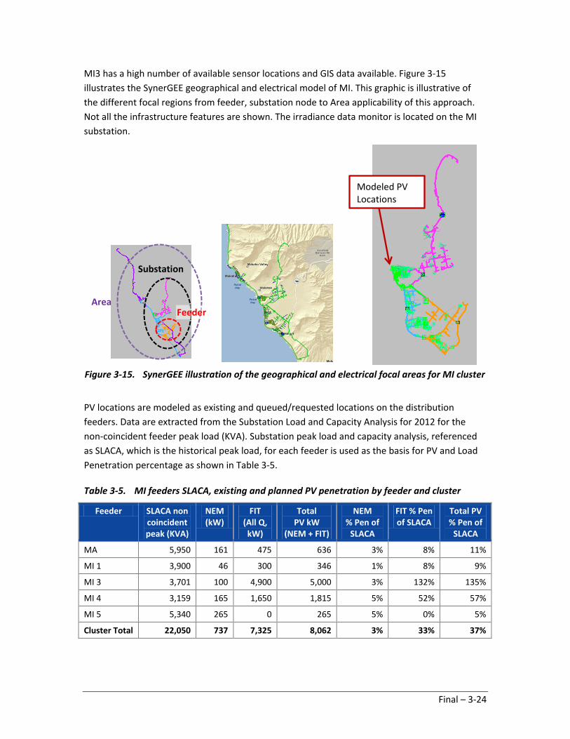
MI3 has a high number of available sensor locations and GIS data available. Figure 3-15 illustrates the SynerGEE geographical and electrical model of MI. This graphic is illustrative of the different focal regions from feeder, substation node to Area applicability of this approach. Not all the infrastructure features are shown. The irradiance data monitor is located on the MI substation.

Figure 3-15. SynerGEE illustration of the geographical and electrical focal areas for MI cluster

PV locations are modeled as existing and queued/requested locations on the distribution feeders. Data are extracted from the Substation Load and Capacity Analysis for 2012 for the non-coincident feeder peak load (KVA). Substation peak load and capacity analysis, referenced as SLACA, which is the historical peak load, for each feeder is used as the basis for PV and Load Penetration percentage as shown in Table 3-5.

Table 3-5. MI feeders SLACA, existing and planned PV penetration by feeder and cluster

Feeder SLACA non coincident peak (KVA)

NEM (kW)

FIT (All Q, kW)

Total PV kW

(NEM + FIT)

NEM % Pen of

SLACA

FIT % Pen of SLACA

Total PV % Pen of

SLACA

MA 5,950 161 475 636 3% 8% 11%

MI 1 3,900 46 300 346 1% 8% 9%

MI 3 3,701 100 4,900 5,000 3% 132% 135%

MI 4 3,159 165 1,650 1,815 5% 52% 57%

MI 5 5,340 265 0 265 5% 0% 5%

Cluster Total 22,050 737 7,325 8,062 3% 33% 37%

Feeder

Substation

Area

Modeled PV Locations

Final – 3-24

The results of each type and stage of analysis are summarized into combined graphs showing the penetration percentage at which either a technical criterion for HECO is violated on the feeder, transformers, or cluster, or there is an indication further study is required. As exact penetrations are not considered in every case, a range of PV penetration as a percentage of SLACA is given in Figure 3-16.

NCM = Non-Coincident Maximum feeder load; Non-Coincident Minimum = Each feeder independent minimum load. FC = fault current. XFMR = transformer

Figure 3-16. Penetration percentage for technical criteria violation on feeder, transformers, or cluster

Final – 3-25

The results are then combined and plotted in order of PV% limitation using the lowest limits from the graphs above (Figure 3-17).

Figure 3-17. Combined penetration limits graph for MI feeders, transformers, and cluster

Each bar in Figure 3-17 represents the lowest percent penetration at which an issue occurred or further investigation is required. Red bars are transformer issues, yellow feeder, and blue cluster level. The X axis is percentage penetration of SLACA.

The green line shows where 15% penetration is in comparison to the highlighted issues, the red line is showing 50% of minimum daytime load for each of the respective items, showing a comparison between the two filtering screens commonly used in both Hawaii and California. The first issues shown are potential for LTC cycling and all occurred above 15% of feeder peak load penetration but below 50% of minimum daytime load. Two different feeder loads are used to test the solar penetration impacts. The first is the 15% of feeder peak load that can occur at any time of the day. The second is the 50% of the minimum daytime load to more closely match minimum feeder load to maximum solar generation.

3.3.2.2 HELCO ML Substation

ML substation is located on the Big Island of Hawaii. ML substation supplies four distribution feeders, ML11, 12, 13, and 14. ML12 is a redundant feeder. The ML feeders supply mainly commercial load, hotel complexes, and associated surrounding demands. The irradiance data monitor is located on the substation.

No distribution model exists for the ML substation. Data are received for the substation in hard copy switching diagram format. The hard copy is a background, and the line topology is traced

Final – 3-26

to enter into SynerGEE. Line construction and type is entered manually from the switching diagram. Other information is provided on PV locations, PV inverter and panel type for existing locations, switch location and type, connected distribution transformers (used for load allocation), and other protection and switchgear information. Substation transformer datasheets are also provided. The ML feeders modeled in SynerGEE are shown in Figure 3-18

Figure 3-18. ML SynerGEE model

The overall trend for both transformers is the tap position decreasing as PV generation increases. The trend is more dramatic for the ML 11 and 12 transformers; above 2,000 kW of PV, the transformer tap position is at its lower limit of -16 (Figure 3-19). The load tap changer is trying to lower high voltages caused by a very high penetration of PV generation on ML 11.

PV Location

Final – 3-27

Figure 3-19. ML12 (top) and 14 (bottom) transformer tap position vs. PV penetration %

-18

-16

-14

-12

-10

-8

-6

-4

-2

0

00%

540.7%

1091.4%

1632.0%

2172.7%

2723.4%

160020%

320040%

480060%

640080%

8000100%

Tran

sfor

mer

Tap

Pos

ition

Installed PV Capacity (kW) Installed PV Capacity (%)

Feeder ML12

Peak Load Min Load

0

1

2

3

4

5

6

7

00%

783%

1566%

2349%

31212%

39016%

50020%

100040%

150060%

200080%

2500100%

Tran

sfor

mer

Tap

Pos

ition

Installed PV Capacity (kW) Installed PV Capacity (% of Peak Load)

Feeder ML14

Peak Load Min Load

Final – 3-28

3.3.2.3 MECO WA Substation and Feeder

WA substation currently has the fifth highest PV penetration on the island of Maui, and GIS and SCADA are available. WA substation currently is connected to 10 PV sites, with a 6.5% penetration level (of peak demand). The peak demand on the feeder is 2,775 kVA, and the minimum daytime demand is recorded as 1,572 kVA, based on 2012 historical annual data. Figure 3-20 shows the SynerGEE electric model of WA substation. The irradiance data monitor is located on the substation.

Figure 3-20. SynerGEE electric model of WA substation

Current flow and percent loading of conductors are monitored at 13 points along the three-phase trunk of the feeder. A peak load with no PV scenario is the base case. For minimum load and 30% PV scenario, there is no back-feeding at the start of any feeder. Each feeder exhibits local reverse current flow on the three-phase main feeder trunk line due to excess PV generation on single phase and two phase lateral taps from the main truck. Table 3-6 shows an estimate of the portion of each feeder’s main trunk that exhibits reverse current flow during different time periods. The figure provides information on the percentage of the line impacted

Final – 3-29

by reverse power flow and potential problems with line regulators, capacitors and fuse coordination as a result of varying power flow along the feeder.

Table 3-6. Estimate of portion of feeders trunk with reverse current flow for WA analysis

WA Substation Feeder % of 3 Phase Trunk with Reverse Current Flow

CKT 1280 21%

CKT 1281 24%

CKT 1320 20%

CKT 1321 —

CKT 1395 14%

CKT 1396 —

3.3.2.4 HECO WO Substation and Feeder

Figure 3-21 shows how the PV locations are mapped and transferred to the model.

Figure 3-21. WO 3 geography of PV locations

WO 3 is an 11.5 kV distribution feeder connected to the WO 46 kV substation. The irradiance data monitor is located on the substation. Transformer 1 serves WO 1 and 2 feeders with power supplied by the IW 46 kV 2 line. Power to Transformer 2 is supplied by the SK 46 kV line and serves the WO 3 feeder (the feeder of interest) and WO 4. Currently WO 3 has 9% PV penetration of peak feeder load and 4.8 MVA peak demand. HECO provided 5-minute peak day (August mid-day) and minimum load day (Sunday afternoon in August) for the two substation transformers. The profiles are aggregated to the 11.5 kV level based on SLACA (HECO’s Substation Load and Capacity Analysis system) loading information. Figure 3-22 shows the peak and minimum day.

Final – 3-30

Figure 3-22. WO feeders load, maximum left-hand side and minimum right-hand side

Figure 3-23 shows the value of kW flow at the substation for varying levels of PV penetration. Any positive kW value represents normal power flow direction, and any negative value represents backflow caused by high PV power output. The point at which the trend lines cross below 0 kW is the moment when backfeed first occurs; this is circled in black for each loading condition. The backfeed occurs at approximately 3,067 kVA for the 40% of midday peak load case, 5,244 kVA for the August peak load time, and approximately 6,789 kVA for the August day minimum load hour.

Figure 3-23. WO 3 backfeed analysis for three loading conditions

Back-feed Point

Final – 3-31

With all PV penetration levels analyzed in the backfeed scenario, the maximum voltages do not indicate potential over-voltage problems. The midday 40% of peak load results show that backfeed may occur during a low load day at the 30% PV capacity penetration level.

The existing inverters and 30% penetration scenarios are used on the WO 3 feeder analysis to perform fault current contribution analyses. The existing PV sites are connected in random order and PV is increased to 30% peak penetration. The actual kVA installed is presented in Table 3-7.

Table 3-7. kW installed kva installed on WO 3

Installation Number kVA installed

1 106

2 13

3 10

4 90

5 22

6 30

7 52

PV penetration increments are simulated on WO 3 feeder, similar to the initial load flow analyses. The results show the percent increase of the greatest symmetrical fault current on the feeder for existing and potential PV generation capacity relative to the no PV case, as shown in Figure 3-24.

Figure 3-24. Maximum % fault current increase for WO 3

Final – 3-32

The total fault current increases by 1.1% from the no PV case to the 30% PV penetration case. This increase is well within the 5% level as set by California Rule 21.

3.4 Conclusion

This component of the CPUC CSI RD&D Solicitation 1 research project studies existing feeders with high penetrations of distributed solar and identify the missing distribution modeling data, determine the most typical studies conditions for evaluating solar, and highlight important factors for utilities to study high solar penetrations. The research team identified six goals for the project and each of these is briefly discussed below.

1. Goal: Identify high penetration analysis needs (load flow, characteristics of the load,protection/coordination, voltage regulation, and islanding) for the distribution circuits beinganalyzed.

Results: Following the feeder studies for SMUD, HECO, MECO, and HELCO, the major feedercircuit evaluations should consider, steady-state distribution simulations, voltageregulation/impacts, frequency impacts due to varying solar generation, islanding andbackfeed into the substation. Time sequential simulations of solar variability over the on-peak periods should be considered for the minimum daytime peak and maximum daytimepeak periods. These time periods have high solar generation with varying cloud densitiesthat impact solar generation. It is determined that a single feeder should not be the onlyconsideration when studying solar impacts. The utility planner must also consider theimpacts to distribution feeders connected to the same substation bus to determine ifbackfeed from one feeder impacts the other feeders.

Fault current, harmonics, protection and transformer load-tap-changers should beconsidered for further in depth studies if there are potential or actual solar inverter impactsto the system. These specific studies are not required for screening or determining feederpotential impacts. These require more detailed data collection and modeling that is notrequired for high solar impact analysis.

2. Goal: Identify additional data parameters to be collected and locations along the highpenetration distribution circuit to place additional high-fidelity monitoring equipment, asnecessary.

Results: Even though a utility planner may be using distribution planning models in dailystudies, the data requirements for modeling solar inverters, gross and net loads,transformer and tap-changer, capacitor bank parameters and distributed load across thefeeder are not included in the standard distribution data sets. The planner must becomemore aware of the distribution of the customer load along the feeder and match new solarinstallations to the location of load. Since distributed solar is being installed on buildings, itis important to match load and solar for accurate simulating of power flows. Many plannersdo not consider transformer tap-changer operations since there are numerous factors that

Final – 3-33

cause tap changer operations. However, during highly solar variability periods, the tap changers could experience excessive tap operations that increase maintenance costs and exposure to mechanical failures.

The collection of high-fidelity solar and power data is very important and is something new to the distribution planner. The planner must study the distribution of load and solar installations to determine the optimal locations to place monitors and sensors. A separate report was prepared for the CPUC by DNV KEMA describing the methodology for locating monitors and sensors on a distribution feeder2.

3. Goal: Record and collect at a minimum 6 (preferably 12) months’ worth of high-fidelity load data from the newly installed high-fidelity monitoring equipment.

Results: The installation of monitors and sensors has been a time consuming task. Security, safety, availability of sites, and selection of proper communication equipment have created delays in beginning feeder studies. There have been communication equipment failures and data losses resulting in sporadic missing data that eliminates potential time periods of interest. The planner must take the time to preplan the selection of sensor and monitoring equipment, communication techniques and data storage.

At HECO, a solar monitor was to be placed at the substation,however, the metalstand would need to be tied to the substation grounding mat. Staff personnel had to be considered along with moving the equipment around the substation yard. The metal stand was replaced with a plastic container to meet safety and security concerns. At SMUD, data was being collected but not communicated back to the control room for one site. It was discovered that animals had chewed through the communication cables.

In collecting solar and load data, the planner must decide on the frequency of data collection. In this study, data was collected in 1-second, 5-second, 15-minute and 1-hour increments. To create consistency of data for feeder analysis, data had to be converted into different time increments. The final data increments changed the simulation analysis. For example, if the data were in 15-minute or hourly increments, the impacts to tap changers and solar variability were very limited in scope or eliminated from the analysis.

4. Goal: Collect electrical equipment nameplate data from the distribution system being analyzed: including distributed generation on the circuit, inverters, any energy storage, circuit size, circuit length, circuit loading, switchgear, and transformers to be used in the model development.

2 Appendix A of http://www.calsolarresearch.org/images/stories/documents/Sol1_funded_proj_docs/SMUD/2011_SMUD_Hi-Pen-PV-Init_Base-Line-Model-final.pdf

Final – 3-34

Results: As stated in Goal #1, compared to traditional distribution studies, there is a tremendous increase in data collection and documentation starting at the substation transformer to the last line segment on the feeder. Each feeder line length, conductor size, phase loading, single taps off the main trunk, capacitor bank operating characteristics, and fuses had to be considered in the expansion of the data sets. The planner must make a list of data requirements that could and did cause in this study for field verification of equipment. Failure to understand the increase in feeder data can cause delays in starting feeder studies.

5. Goal: Investigate varying incremental levels of PV penetration at the distribution capacity level and iterate with an existing system level model to understand to what degree higher PV levels will adversely affect the grids.

Results: In this study, the distribution feeders were studied under varying solar penetrations from “no PV” to 100% of peak PV penetrations. The results indicate that there is no set penetration limit for feeders but the penetrations vary widely due to load and solar locations, feeder conductor sizes, and other factors. Some feeders experienced issues at 30% penetration while others could have as high as 100% penetration. The penetrations varied by study parameters such as backfeed, voltage, frequency, etc. Each had solar penetration limits that would need to be mitigated through feeder upgrades or other options.

6. Goal: Based on the validation results for a single circuit study, develop a methodology for extending the findings using the simulation tools to inform and expedite interconnections studies at higher penetration levels.

Results: The report discusses methodologies for studying high solar penetrations. The simulation tools are an important consideration before starting feeder studies. Some distribution simulation tools such as SynerGEE cannot model inverters while others such as CYME can but requires additional module purchases. In order to simulate inverter impacts on an unbalanced distribution feeder, the feeder is converted to a balanced feeder and imported to a transmission model such as PSS/E or PSLF, used by SMUD and HECO, respectively. This conversion eliminates the single phase issues that are important for distribution penetration studies but is adequate for screening analysis.

Table 3-8 summarizes the general findings from the study. The results are based on steady-state and first contingency analysis. The areas in red indicate feeder conditions impacted by high penetrations of distributed solar. The main conditions impacted are high voltage and backfeed onto the feeder. The blue areas indicate potential areas of concern as distribution solar penetrations increase. These areas are potential line segment overloads and excessive LTC operations.

Final – 3-35

Table 3-8. Study summary

Feeder Utility Voltage (kV)

Customer Mix

PV Pene-tration

Line Loading

LTC Operation

Voltage Backfeed

A-C (3 feeders)

SMUD 12.47 Res 0% to 100%

No violations

N/A High voltage

High backfeed

RF (1 feeder)

SMUD 12.47 Com/Ind 0% TO 88%

No violations

N/A No violations

No violations

EB (1 feeder)

SMUD 12.47 Rur 67% No violations

N/A High voltage

High backfeed

CT (2 feeders)

SMUD 12.47 Res/Rur 0% to 50%

Potential for

overloads

Minor operations

High voltage

No violations

EG (3 feeders)

SMUD 69 Res/ Com/ Rur

38% to 60%

No violations

Minor operations

No violations

No violations

L7 (1 Feeder)

SMUD 69 Ind 0% TO 150%

No violations

N/A No violations

No violations

MI (4 feeders)

HECO 11.5 Res/Com 9% to 135%

Potential for

overloads

Potential cycling

High voltage

High backfeed

ML (4 feeders)

HELCO 4.16 Com 0% to 100%

No violations

Potential cycling

High voltage

High backfeed

WA (6 feeders)

MECO 13.09 Res/Com 0% to 30%

No violations

N/A No violations

No violations

WO (5 feeders)

HECO 11.5 Res/Com 0% to 40%

No violations

N/A No violations

Potential for

backfeed Res = Residential Ind = Industrial Rur = Rural Com = Commercial

Final – 3-36

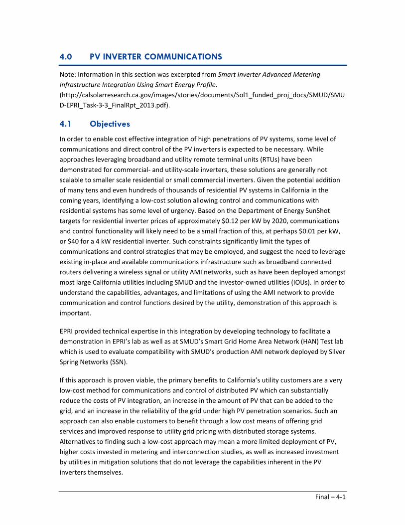
4.0 PV INVERTER COMMUNICATIONS

Note: Information in this section was excerpted from Smart Inverter Advanced Metering Infrastructure Integration Using Smart Energy Profile. (http://calsolarresearch.ca.gov/images/stories/documents/Sol1_funded_proj_docs/SMUD/SMUD-EPRI_Task-3-3_FinalRpt_2013.pdf).

4.1 Objectives

In order to enable cost effective integration of high penetrations of PV systems, some level of communications and direct control of the PV inverters is expected to be necessary. While approaches leveraging broadband and utility remote terminal units (RTUs) have been demonstrated for commercial- and utility-scale inverters, these solutions are generally not scalable to smaller scale residential or small commercial inverters. Given the potential addition of many tens and even hundreds of thousands of residential PV systems in California in the coming years, identifying a low-cost solution allowing control and communications with residential systems has some level of urgency. Based on the Department of Energy SunShot targets for residential inverter prices of approximately $0.12 per kW by 2020, communications and control functionality will likely need to be a small fraction of this, at perhaps $0.01 per kW, or $40 for a 4 kW residential inverter. Such constraints significantly limit the types of communications and control strategies that may be employed, and suggest the need to leverage existing in-place and available communications infrastructure such as broadband connected routers delivering a wireless signal or utility AMI networks, such as have been deployed amongst most large California utilities including SMUD and the investor-owned utilities (IOUs). In order to understand the capabilities, advantages, and limitations of using the AMI network to provide communication and control functions desired by the utility, demonstration of this approach is important.

EPRI provided technical expertise in this integration by developing technology to facilitate a demonstration in EPRI’s lab as well as at SMUD’s Smart Grid Home Area Network (HAN) Test lab which is used to evaluate compatibility with SMUD’s production AMI network deployed by Silver Spring Networks (SSN).

If this approach is proven viable, the primary benefits to California’s utility customers are a very low-cost method for communications and control of distributed PV which can substantially reduce the costs of PV integration, an increase in the amount of PV that can be added to the grid, and an increase in the reliability of the grid under high PV penetration scenarios. Such an approach can also enable customers to benefit through a low cost means of offering grid services and improved response to utility grid pricing with distributed storage systems. Alternatives to finding such a low-cost approach may mean a more limited deployment of PV, higher costs invested in metering and interconnection studies, as well as increased investment by utilities in mitigation solutions that do not leverage the capabilities inherent in the PV inverters themselves.

Final – 4-1

4.2 Approach

This demonstration was configured to use the typical communications architecture implemented by SMUD for demand response field implementations. The equipment and software used was existing infrastructure with the following exceptions:

1. The SMUD test facility did not have suitable solar panels or solar simulator available, so a direct current (DC) power supply was used as a substitute.

2. EPRI developed a Smart Energy Profile (SEP) Gateway described later in this report to translate the Smart Energy Profile (SEP) 1.x commands in the Fronius interface protocol. SEP 2.0 will provide many of these functions but was not available in time for this work.

3. Test certificates were used rather than production certificates since the EPRI SEP Gateway was a prototype unit.

The idea behind the implementation of smart inverter control using SEP 1 is to use the existing message structure to support distributed energy resource control and monitoring. Since SEP 1 did not have native commands to accomplish these functions, it was necessary to select substitute functions that could be repurposed. EPRI provided a SEP Gateway to accomplish the tasks of translating the SEP 1 demand response/load control (DRLC) and metering commands into messages that the Fronius smart inverter understands and implementing the messages in the Fronius interface protocol.

4.2.1 Test Architecture

Testing was conducted at two locations: (1) the SMUD facility at 6201 S Street, Sacramento, California, and (2) the EPRI Laboratory in Knoxville, Tennessee.

Testing using utility equipment was conducted at the SMUD facility. The equipment arrangement for the testing at the SMUD facility is shown in Figure 4-1. This demonstration test was conducted in SMUD’s Smart Grid HAN Compatibility Lab on April 23, 2013. A DC power supply was used to replace a PV source for the inverter in both test setups due to unavailability of a suitable PV source at the test facilities. Because the focus of this effort was on the capabilities and limitations of the AMI network for delivering control signals, this choice of power supply did not impact any of the research objectives. Curtailment of PV generation is a capability of PV inverters that has been required for maintaining grid stability in places with high penetrations of PV such as Germany (Barth, Bianca; Franz, Oliver, Results of PV Grid Research for Germany, October 2013, presented at European PVGrid Forum.

Final – 4-2

Figure 4-1. Testing at SMUD facility

EPRI developed an interface device that enables connectivity of the inverter to the HAN of a meter in an AMI system. Figure 4-2 depicts the test arrangement used during development by EPRI. SSN provided a field service unit (FSU) to act as their interface to the EPRI SEP gateway.

Figure 4-2. Testing at EPRI Knoxville Laboratory

Silver Springs Web Interface (HCM)

ZigBee 1.1 Residential Meter

EPRI SEP Gateway

300VDC Power Supply PV Simulation

Fronius Inverte

IEEE 802.15.4

SSN 900MHz Mesh

RS422 SSN Network Servers in San Diego

Wireless Access Point

ZigBee Meter Simulator PC

SSN FSU ZigBee 1.1 Module

EPRI SEP Gateway

IEEE 802.15.4

USB

RS422

300VDC Power Supply PV Simulation

Fronius Inverter

Final – 4-3

Table 4-1 is a list of the equipment used for the demonstration tests.

Table 4-1. Equipment list

Device Description

Inverter Fronius IG Plus V 3.0-1 UNI rated at 3 kW PV with maximum power handling capability of 4 kW

DC Power Supply TRC Model TCR500T20-1 capable of 500 VDC at 20 amperes maximum

SEP Gateway Device constructed by EPRI to perform protocol translation between ZigBee 1.1 to the Fronius interface protocol

Electrical Meter Landis and Gyr Focus AX with Silver Spring Networks NIC, FW version UtilOS v2.10.6c

Headend System Silver Spring Networks UtilityIQ v4.2.14

Headend System Silver Spring Networks HAN Communication Manager v1.7.2

SSN FSU Silver Spring Networks HAN Test Kit

4.2.1.1 SEP Communications

The test is designed to use the currently deployed hardware and software used by SMUD as shown in Figure 4-1. A key element of this demonstration is the repurposing of SEP 1 DRLC and metering functions to be used for control and monitoring of smart inverters.

4.2.1.2 Device Join

Low level communication between the gateway and the meter is handled by the ZigBee protocol as outlined in ZigBee document 1_053474r17ZB_TSC-ZigBee-Specification.pdf (available at http://www.zigbee.org). Creating the ZigBee network or "joining" the meter and gateway is handled in hardware by placing the both devices in join mode. Once the network is formed, the devices can exchange application layer messages.

4.2.1.3 Device Operation

Application layer messages follow SEP version 1.1 which defines the DRLC and Metering clusters. The ZigBee website (http://www.zigbee.org) provides additional information:

• SEP is defined in the ZigBee document 084956r05ZB_ZSE-Smart_Energy_Specification_Package.pdf.

• SEP uses and extends the standard ZigBee clusters defined in the document 075366r01ZB_AFG-ZigBee_Cluster_Library_Public_download_version.pdf.

The gateway polls the Fronius inverter every 5 seconds, alternating between reading watts (W) and total watt-hours (Wh). It creates 15-minute intervals that can be read via the ZigBee simple metering cluster. The current implementation only reports one interval at a time, regardless of how many intervals are requested. The previous 24 intervals are stored and can be queried one at a time.

Final – 4-4

On startup, the gateway sets the inverter to 100% generation. If the connection to the ZigBee network is lost and an event is in progress, the inverter generation reverts to 100% output.

When an inverter output reduction is desired, a DRLC event is sent to the SEP Gateway. To control the amount of generation, the duty cycle parameter in the DRLC message is set to control percentage output. Acceptable values are between 0 and 100% with 100% being full output from the inverter. Any power request below 10% is treated as a shutdown by the Fronius inverter. This is a function of the inverter and not the EPRI gateway module.

The gateway implements the simple metering and DRLC clusters from ZigBee 1.1. Data read from the inverter are in watts, while the ZigBee network expects an integer value in kW. To prevent losing precision due to rounding, the readings from the inverter are reported in watts and the appropriate metering divisors are set to 1,000. This is the normal method used by SEP 1.1 to maintain reading accuracy when dealing with a wide range of returned values.

The gateway can connect to a computer via a universal serial bus connector for purposes of accessing debug messages generated during the test process. It provides information on the ZigBee connection status, power generated by the inverter, and message logging for events.

4.2.1.4 Processing DRLC Events

When the gateway boots or connects to a ZigBee network, it first performs time synchronization, and then queries for active events. It only stores one event at a time. When an event ends or is canceled, the device will query for another event. If the ZigBee network connection is lost, any stored events are cleared, and any in progress events are canceled.

4.2.1.5 Processing Simple Metering Queries

The gateway responds to load profile requests, but will only return one interval at a time in 15-minute intervals.

The gateway is capable of supporting the following attributes from the SEP 1.x metering cluster:

• Summation delivered (0x0000)

• Summation received (0x0001)

• Instantaneous demand (0x0400)

• Unit of measure (0x0300)

• Divisor (0x0302)

• Summation formatting (0x0303)

• Demand formatting (0x0304)

• Metering device type (0x0306)

Final – 4-5

See the ZigBee Smart Energy Profile Specification, document 075356r16ZB, for a description of these attribute/reading information set identifiers. These values would be defined in the gateway for fixed values read from the inverter for measured values such as instantaneous demand. The data can then be reported to the SSN headend using the metering cluster.

4.2.1.6 Time Synchronization

Upon joining a ZigBee network, the gateway queries the network for the current time. Time synchronization is repeated every hour thereafter.

4.2.2 Inverter Communications

Two control functions were implemented: output limiting as a percentage of maximum output and inverter shutdown. A single control message provides functionality to set the output level to a desired percentage of maximum or shut the inverter down completely. The output level can be set to any value between 10 and 100% of maximum output. Any request to limit the output to less than 10% of the maximum will result in an inverter shutdown.

Two monitoring functions were implemented:

• Historical Meter Data – This provides the amount of PV power generated in 15-minute blocks.

• Instantaneous Power – This provides the amount of PV power being generated at the instant that the request was received.

The Fronius IG Plus V inverter communicates via a proprietary Fronius interface protocol running over a full duplex RS422 connection. This protocol is described in detail in 42_0410_1564_168027_snapshot.pdf available from Fronius.

For this demonstration, only three basic functions were used. The first two are the Get power – Now command to read the instantaneous power and the Get energy – Total to read the total watt hours produced. These were used for the monitoring functions described above. The Set Power Reduction function was used to limit the output power and to shut down the inverter.

4.2.3 Test Equipment Arrangement

4.2.3.1 Inverter Power Connection Details

Figure 4-3 shows a simplified power wiring diagram for the test configuration.

Final – 4-6

Fronius Inverter

208 VAC 3 Phase

Circuit Breaker Limit Power to 4kW

TCR DC Power Supply

250 VDC 16A Max

208 VAC Single Phase

Circuit Breaker Limit Power to

3kW

AC Grid Connect

DC PV Input

Figure 4-3. Power wiring diagram

The inverter was connected to the grid via a single phase 208 VAC 60 hertz tie into a panel through a breaker to limit the maximum power supplied to approximately 3 kW. The PV supply was simulated by a DC power supply. This DC supply is connected to a three-phase 208 VAC source via a circuit breaker limiting maximum power to 4 kW.

Figure 4-4 shows the inverter lying on top of the power supply cart. All testing was done in this configuration.

Figure 4-4. Inverter and DC power supply

Grid Power Connect Block

Final – 4-7

The wiring terminal block is visible at the end of the inverter facing the camera. The first is a view inside through the open lid and the second is from the bottom looking in through the wire exit. The bottom cable plate has been removed for a clear view of the terminations.

Figure 4-5 shows the unit after connection. The grid connection is in the bottom right of the image in the order ground, L1, L2, and neutral. The blue wire above the grid connection is the RS422 communications cable. The black cable to the left of the grid connection is the plus and minus of the DC power supply.

Figure 4-5. Inverter with power and communication connections

4.2.3.2 Testing Performed at SMUD

The testing performed at SMUD was done using 208 VAC phase-to-phase with neutral and ground for the grid connection. The SEP message source was SSN UtilityIQ v4.2.14 communication through a Landis and Gyr Focus AX electric meter with SSN NIC, FW version UtilOS v2.10.6c. Test certificates were used for all steps.

The test steps performed were power limiting and inverter shut down.

4.2.3.3 Testing Performed at EPRI

The testing performed at EPRI was done using 240 VAC split phase with neutral and ground for the grid connection. The SEP message source was SSN simulator system using a Linux application to generate messages. Test certificates were used for all steps.

The test steps performed were historical data collection and instantaneous power acquisition.

Final – 4-8

4.3 Findings

4.3.1 No Significant Issues

There were no significant issues in using SEP 1.1 to control a smart inverter by re-purposing the DRLC and meter reading functions. In this case, the duty cycle value was used to contain the percent output where 100% was the maximum output from the inverter.

After an initial successful join of the gateway, some connection issues were encountered after this join was lost. These issues were resolved after the HAN communication manager was forced to un-join from the meter and gateway. After forcing the un-join the gateway and the meter joined without problems.

The inverter was constantly searching for the optimum power output from the solar panels. Because a DC power supply was used as a simulated solar source, the power output of the inverter was not steady; it varied by up to 200 watts. With this taken into consideration, the values returned were well within expected accuracy.

This was a test of communications and as such the results were positive. Power output from the inverter was limited to 2,000 watts while at SMUD because of the use of a 208 VAC grid connection combined with a DC power supply used to simulate a PV array. When this inverter was used at the EPRI laboratory driven by a commercial solar simulator, the full power range of the inverter up to 4,000 watts was available.

During the testing the inverter would occasionally display “DC side low" when a DRLC event ended. This seems to be an issue of using a DC power supply for the simulated PV input. This was never an issue when testing in the Knoxville Laboratory using a commercial PV simulator or actual PV panels as a power source. This is likely caused by the DC supply not responding quickly enough, causing the inverter to go into a restart mode. This has no impact on the success of the communication test since there is a high level of confidence that the system will operate normally with PV power source.

As a proof of concept, this demonstration verified there are no technical issues to prevent the control of smart inverters using the DRLC and metering commands built into SEP 1.1. This demonstration did not address the operational issues that would be encountered re-purposing these commands.

4.3.2 Implications for Widespread Deployment

One of the objectives of this research was to improve understanding of the capabilities, advantages, and limitations of using the in-place AMI network to accomplish communications and control functions with a widespread deployment of smart residential PV inverters.

Final – 4-9

4.3.2.1 Cost Implications of AMI Network Smart Inverter Communications

Some advantages of this approach were understood at the outset, primarily that the communications infrastructure had already been paid for and deployed through SMUD’s SmartGrid project, and as such, so long as inverter communications did not overwhelm the system capacity, infrastructure costs would be minimal. As envisioned, the only hardware to enable inverter communications would be a ZigBee-compatible device in the form of either the inverter itself with an embedded chip or a gateway as demonstrated in this project. As a result, achieving broad communications with residential inverters could be inherently low cost given the expected costs of ZigBee chips are expected to be on the order of a few dollars per unit.

Other advantages lending themselves to this approach were the interfaces that have been developed to support Demand Response functionality that can be leveraged for communicating with inverters using the same protocols, namely SEP. In addition, tools are in place with SSN such as UIQ (formerly known as User Interface Quartz), for communicating with thermostats and other in-home devices that make use of the SEP standard, that offer scheduled and real-time two-way communications with many thousands of devices at once. These systems currently talk to SMUD meters on regular polling schedules, typically every 4 hours for residential customers, and more frequently for commercial, to collect usage data. They are also used for service shut-offs and other demonstration project purposes at this point. Finally, mesh network offers some inherent reliability due to redundancy of the communications pathways afforded in a mesh. Typically a single wireless access point (WAP) will attempt to reach a meter three times before a similar attempt is made from a neighboring WAP, also up to three times. Communications rates for SMUD’s meters through the SSN network are currently 97% on the first attempt, and 99.9% for an entire 3-minute cycle of six reads from two different WAPs.

4.3.2.2 Functionality Considerations

In terms of the capabilities, the demonstration itself was limited to the functions that are supported by SEP 1.1 and the DRLC. As such the functions were limited to curtailment and monitoring functions and did not include any of the more advanced voltage control and storage related functions that are supported in SEP 2.0. Once SEP 2.0 is deployed on SMUD’s AMI network, however, it is expected that these and other functions will be supported. Beyond the specific functions, the demonstration showed fast and reliable response to the control signals that were sent, typically seeing response by the inverter on the order of 1 to 3 seconds after a command was sent. This responsiveness is impressive considering the signal was routed through the web and the SSN servers in San Diego, back up through SMUD’s WAP, through the meter and gateway to the inverter. Such responsiveness suggests the potential for real-time command signals to be sent out that could affect changes on a system in response to very short-term needs of a utility related to unexpected or forecasted changes in available generation or significant swings in demand.

However, consideration also needs to be made for the technology constraints associated with scheduling events with such high frequency. The UIQ system was not designed for broad

Final – 4-10

communication and execution of different functions on a minute-to-minute basis with hundreds of WAPs. Based on discussion with SSN representatives, such levels of communication would likely overwhelm some of the design constraints of the UIQ system; they were much more comfortable with a time frequency closer to 5 minutes relative to the capabilities of the system.

4.3.2.3 Security Considerations

Despite the apparent advantages from a cost and functionality standpoint for achieving relatively high frequency, reliable communication with potentially tens of thousands of devices, there are security considerations that need to be addressed with this approach. For any device connecting to the network, separate testing for compatibility with SSN and ZigBee must be done. Security concerns arise due to the potential for accessing SMUD’s network and compromising data, system reliability, and potentially violating regulatory requirements with NERC. For any upgrades to the inverter firmware, re-testing would need to occur to ensure compatibility and security requirements are maintained. Currently, costs for these tests are on the order of $20,000 per test, which is potentially cost-prohibitive without significant scale in the number of devices deployed. Such considerations make it difficult to envision a system where tens of device manufacturers were able to maintain up-to-date testing and security requirements without significantly adding to the costs of devices. However, promising approaches are being pursued by EPRI to make use of a common interface gateway that would enable communications with a variety of consumer appliances and would effectively enable a single device to be tested and used for communications in each utility smart grid deployment with interoperability specific to that utility. SMUD is pursuing demonstration of this type of a product with EPRI and others—including SunSpec, Sandia, SCE, TÜV Rheinland, and Xanthus Consulting—to reduce concerns about costs of meeting security requirements and to reduce the costs associated with enabling utility communication with a variety of consumer devices.

4.3.2.4 Bandwidth, Latency, and other Potential Limitations

Another potential disadvantage of this approach is that the nature of the mesh network as designed does not assure certainty of delivery of control signals. Generally, this effect gets worse as the number of devices per WAP increases and as the time frequency of communication decreases. Currently SMUD’s system is designed fairly conservatively, with approximately 5,000 devices per WAP, which enables the system to achieve a 97% communications success rate on the initial attempt, and 99.9% after the sixth attempt, which occurs in a 3-minute cycle. According to SSN, typically 95% of the devices receive a signal within about 1 second on the system. The system makes use of approximately 50% of its theoretical capacity for the first 20 to 30 minutes of a 4-hour read cycle, with the majority of that amount being taken up by protocol overhead. The PV transactions would not be expected to increase the overhead and would have a comparable impact as the metering transactions, which as noted above is quite small. As a result, SSN expects that the addition of up to 50,000 PV inverter devices (1/10th the number of existing meter devices), communicating at 50 times the frequency (every 5 minutes as opposed

Final – 4-11

to every 4 hours), and passing 3 to 5 data points per communication, would not have a significant impact on the system bandwidth.

In the event that issues are identified with unacceptable levels of failed communications, addition of WAPs to the system would alleviate congestion and enable higher communication rates. Generally, costs for additional WAPs are dominated by design and installation costs rather than hardware costs and in total may range from $7,000 to $12,000 installed, with an additional $30 to 50 per month wireless fee. Conditions where an additional access point might be required are only anticipated to occur in large communities with very high penetrations of solar homes. While potential bandwidth and latency constraints can be addressed by deployment of additional WAPs on the network, valuation of achieving higher certainty of receipt of signals by all units compared to the cost of the additional WAPs has not been done, and requires far more information about the value of services that could be provided by the PV devices than is available today. Exploration of this will require extensive further research, including valuation under various scenarios of scaled deployments and considering a variety of control functionality that might be desired. Alternatives to deal with this issue are to develop and deploy localized control schemes at the inverter that can be selected periodically by the utility to address concerns related to variability, voltage control or backfeeding of the substation, which may prove more cost effective than enhancements to the AMI network. In addition, these localized control strategies are likely to be more desirable to system operators given the complexity of coordinating tens of thousands of small units on a high frequency basis.

4.3.3 Findings and Other Considerations

Based on discussions with SMUD and SSN staff, it does not appear that anticipated high penetration PV scenarios currently contemplated present any significant challenge to the existing network performance. Security issues may be a challenge to address but are likely substantially mitigated by moving to a standardized multi-appliance gateway device for the interface. Such an approach was recently awarded funding under CSI RD&D Solicitation 4 for development and demonstration led by EPRI with project partners SMUD, SunSpeC, Sandia, SCE, TÜV Reinland, and Xanthus Consulting (http://www.calsolarresearch.org/csi/107-sol-4-test-entry). In the event extremely high penetrations in certain communities do impact performance, additional WAPs can be added at a reasonable cost. Finally, expected autonomous modes may substantially reduce the potential system demands currently being contemplated, rendering even high penetration scenarios extremely unlikely to tax the existing system architecture.

Beyond the approach explored in this research, additional evaluation of alternative pathways such as broadband should be explored to understand advantages and limitations of those pathways. In particular, as micro-inverters begin to take up a larger share of the residential inverter market, broadband communication with PV inverters or residential gateways may become more common place and, as such, might lend itself to being a preferred pathway for devices that may have a lower price point than centralized residential inverters. Some of the perceived limitations of a broadband approach is the lack of a single utility control interface

Final – 4-12

through which devices from a variety of manufacturers could be accessed and controlled, as well as challenges with maintaining or controlling connectivity to the devices, and the potential for increased costs for the services that are enabled by the broadband provider, the router, and the PV inverter supplier. On the other hand, a single-point utility-PV broadband interface could certainly be developed if such a communications pathway presented enough advantages.

Final – 4-13

5.0 SYSTEM INTEGRATION AND VISUALIZATION TOOLS

Note: Information in this section was excerpted from HIP-PV Task 4: Visualization of High Penetration PV, Final Report. (http://calsolarresearch.ca.gov/images/stories/documents/Sol1_funded_proj_docs/SMUD/Task -4_PilotVisual_Final-Report.pdf).

5.1 Objectives

Individually, distributed PV systems are relatively small compared to other generation resources, but add considerable value to the customer. However, in aggregate, the behind-the-meter, the capacities of roof-top installations are becoming as large as some of the utilities’ generators which provide additional grid support and reliability services for the rest of the system. Although distribution circuits are typically capable of withstanding load changes over a range of conditions, the lack of visibility, accurate modeling, and information to monitor and control increasing levels of variable DG resources such as PV systems on the distribution circuits has created increasing reliability and power quality concerns among utility planners and grid managers. Utilities are essentially blind to these behind-the-meter resources and need new data and analytical capabilities and tools to help capture and better understand distribution level impacts, particularly when it comes to demand side resources providing generation onto the grid.

Distribution Interconnection standards in Hawaii (Rule 14H) and California (Rule 21) reference a 15% penetration (of peak) of PV as an initial screen for high DG penetration on distribution circuits. However, both HECO and SMUD are contending with circuits well above 15% of DG generation to circuit maximum load. In Hawaii on the island of Oahu, a handful of feeders are above 100% of circuit maximum. At these penetration levels, traditional rules of thumb for design of protection and distribution systems are reaching their limits or are being compromised but not necessarily monitored by utilities. Additionally, existing load management schemes, including protective load switching on lines and under frequency load shed (UFLS) and outage management schemes designed and implemented prior to the high levels of distributed PV, may no longer be adequate. As PV generation continues to grow on distribution circuits, such grid management and operational schemes as well as the traditional modeling tools will need to be modified to account for DG generation and changing daytime circuit conditions.

As part of the HiP-PV Initiative visualization task, HECO initiated a number of high resolution data monitoring and evaluation efforts on the islands to gain visibility and re-tool planning and inform new operating processes so the existing operational practices can account for high levels of DG penetration. Efforts focused on the development of the following four new visualization capabilities:

• Renewable Data Architecture and Analytics – Common Data Interface Tool

• Location Value Map (LVM) and Online LVM

Final – 5-1

• Renewable Watch

• Operations Integration

This work complements other efforts being pursued as part of the HiP-PV initiative, including modeling, monitoring, and technical outreach. Working with a team of industry partners including Siemens, Alstom, AWS Truepower, DNV, Referentia Systems Inc., and various field monitoring equipment and telecom providers, the new visualization and analytical tools have been developed and piloted as part of this effort and is now being utilized and continuously updated to help Hawaii manage increasing levels of variable renewable resources on the island grids. Results and findings have applicability to mainland grids where distributed generation penetration levels are now beginning to exceed 15% and are projected to grow. Results of this collaborative effort are also expected to have impact internationally as industry partners help to propagate and share results and findings with their customer base.

The scope of the visualization task included the following:

• Assessing System Needs and Strategies

– Convene meetings with system operations staff and capture existing needs

– Identify visual mitigation strategies to bring awareness of system impacts from distributed PV

– Identify important operational strategies that can benefit from monitoring and control of distribution feeder parameters

– Develop and pilot analytical tools to allow evaluation of high penetration PV data to inform modeling scenarios

• Develop, Pilot, and Validate Visualization Tools

– Compile database of solar resources on the distribution system capable of handling high-frequency 1 second data to 15 minute resolution.

– Utilize LVM to identify and track highly impacted distribution circuits and develop automated capability to update and visually track penetration levels

– Develop an operational tool that incorporates field monitoring data, planning data along with live system data to improve awareness of renewable resource availability

– Begin preliminary efforts with energy management system (EMS) vendors to enhance data analysis and use high-resolution solar resource information in the operational environment

– Capture lessons learned through piloting efforts

Final – 5-2

5.2 Approach

The approach for this task can be broken into the following phases: 1) seeing is believing, 2) get data fast, and 3) Information to Action and provide utility operators visibility and tools to accommodate higher penetrations of PV.

Phase 1 – Seeing is believing. A priority goal of the visualization task was to assess and provide visual awareness to the solar resource information and impacts of renewables on operations and planning.

Detailed modeling on high penetration PV feeders conducted as part of the HiP-PV Initiative modeling task (Section 3) showed that while variability of PV resource can be a concern on power quality, there may be greater risk to system operations by not appropriately accounting for aggregated impact of PV generation on system protection, cost-effective reserve management, load forecasting, and load management strategies including under frequency load shed, generator outage events, and system restoration, especially during the daytime. With high levels of both wind and solar, HECO is tracking frequency issues and noting protection device performance concerns, such as LTC for voltage control, at the system level due to variable wind and solar resources at the distribution feeder level (Figure 5-1 and Figure 5-2).

Figure 5-1. System uncontrolled ramp concerns due to solar (source: HELCO)

Final – 5-3

Figure 5-2. Observed increase in local feeder LTC movement due to solar (source: HECO)

Phase 2 – Get data fast became the next priority goal. Like most utilities, communication and secure protocol to backhaul the data is limited at the distribution level in Hawaii. This required innovative solutions that leveraged existing communication infrastructure including the use of a wide range of protocols for microwave, radio, and cellular devices. Working with utility field and instrumentation crews, SCADA-enable solar irradiance sensors and cellular devices to support non-SCADA communication were deployed. Figure 5-3 and Figure 5-4 showcase a variety of solar and wind monitoring devices deployed across HECO and SMUD service territories at substations and strategic monitoring locations.

Figure 5-3. Examples of solar monitoring devices deployed in Hawaii and California

Final – 5-4

Figure 5-4. Remote wind monitoring sensors (SODAR and LIDAR) and temperature profilers

(radiometer) deployed in Hawaii as part of the forecasting network (WindNET)

In Hawaii, to facilitate documentation of different device setups, acronym identifiers were created. For example, reference irradiance sensors that served to join data to transmission infrastructure were identified as TJD. A short description for each sensor is provided below.

• TJD sensors serve as reference sensors. TJD sensors consisting of calibrated Licor 100 irradiance sensors were installed in two configurations, either as a tri-pod stand which left communication antenna, global positioning systems (GPS) and data acquisition (DAQ) devices exposed or used a plastic bin to house antenna, GPS and DAQ at substations more susceptible to vandalism. Complete sensor kits were purchased from Campbell Scientific. TJD devices were sited at utility sites and non-utility sites in consideration of forecasting and grid monitoring needs.

• Locational monitor versions 1 and 2 (LM-1 and LM-2) were deployed at various substations during the project period. Both consisted of using a small PV sensor (0-10 V) which telemetered voltage output data from the panel back to the utility’s data collection systems. LM-1 devices were developed internally by the utility and did not have external calibration. They required a reference source such as a nearby TJD for correlation. LM-2 devices are commercially available, calibrated sensors with both voltage and temperature sensing capability. These devices are distributed by IMT Solar (www.imtsolar.com). Plans are to replace LM-1 with LM-2 as they are easier to install, have digital connection to SCADA via an RS485 connector, and are commercially calibrated.

• SMS are calibrated shadowband sensors for determining components of the total irradiance (direct normal irradiance [DNI] and diffuse irradiance). These stations are Campbell Scientific kits installed by AWS Truepower to support solar forecasting needs. They serve similar purposes as TJD which measures total irradiance. They are part of the SolarNET sensor network for solar forecasting in Hawaii.

Final – 5-5

• SODAR sensors are sonic detection and ranging devices that remotely measure wind speed and direction using sound. SODAR systems were either mobile, PV-powered systems or station powered and are also part of the WindNET and SolarNET for forecasting and cloud modeling in Hawaii. Atmospheric Research and Technology (ART) SODARs (www.sodar.com) and deployment services were used in Hawaii. ART VT-1 SODARs were also used in the California SODAR campaign conducted from 2002 to 2004 by the California Energy Commission. They provide multi-level measurements from ground level up to 300 meters. To minimize noise levels near the areas of deployment, measurements in Hawaii ranged from ground level up to 200 meters.

• LIDAR sensors use light to measure wind speed and direction and provide the capability to scan an area ahead of the wind facilities. The Leosphere WindCube 100S (www.leosphere.com) was deployed by Leospshere, AWS Truepower, and HECO staff on Oahu. The LIDAR is part of the WindNET supporting forecasting.

• Radiometers are remote sensors used to record vertical temperature from the ground up to 1 kilometer (km). A Radiometrics unit was deployed by AWS Truepower for about 9 months on the Big Island and moved to Maui to continue vertical temperature measurements. Data provide a more accurate temperature profile to initiate meso-scale models for forecasting wind for the islands. These devices are part of the WindNet and SolarNet.

• PMI units are commercial power quality monitors manufactured by Revolution (www.powermonitors.com). They were installed by the utility at various customers who were willing to participate and share feeder-level power quality data in support of feeder monitoring and distribution model validation. Data were used by DNV to validate modeling studies and develop high penetration modeling methodologies as part of HiP-PV’s modeling task.

Monitoring sites for various devices were chosen resulting from a combination of factors including proximity to load, unique terrain, microclimate, shading and other structural blockage, and diversity of load types on the circuit. Each site also had unique deployment challenges including limited communication options, threat of vandalism, safety clearance requirements and customer access constraints. Table 5-1 summarizes various means used to access and backhaul data. As both SMUD and HECO began deploying sensors, the management of high resolution data and large volumes of data quickly became an issue.

Final – 5-6

Table 5-1. List of monitoring devices, communication, and data resolution

Field Device Communication Access Data Resolution

TJD Solar Kits – Irradiance (W/m2) Non-SCADA, Cellular 1 min

LM 1 – % availability (%), calibration reference needed

SCADA 2 sec

LM 2 – Voltage to calibrated Irradiance (W/m2)

SCADA 2 sec

SMS Stations • Irradiance (W/m2) components

• Wind mast (m/s)

• Temperature (deg C)

• Pressure (Pa)

Non-SCADA, Cellular 1 min

PMI – power quality (V, Amp, Load) Non-SCADA, Manual data pulls Various (1 - 15 min)

SODAR – volumetric wind data (m/s, direction)

Non-SCADA, Cellular Various (5 min – 15 min)

Radiometer – Temperature (deg C) Non-SCADA, Cellular 1 min

LIDAR – wind data (m/s) Non-SCADA, Cellular Various

Phase 3 – Information to action was the third driving goal. Once data were received, questions arose on how best to combine and mine the data and what utility tools were available to do so. Existing utility analytical tools tended to be software and vendor product specific with data analysis software specific to the device or database. Also, data were stored on multiple databases, formats, required separate logins, and database programming expertise or other department staff with local database access to download and transfer the information. Hunting down and assembling data to perform analytics was a time consuming task often taking several days to weeks before analysis could even begin.

With higher resolution, diverse formats, larger volumes of data, and the future need for real-time streaming of information across SCADA and non-SCADA platforms, the focus of the visualization task activities that followed was to enable flexible and secure access to information on a common platform and to flexibly render large volumes of data in a graphical and visual way. To enable a common platform and visualization capabilities, the Hawaiian Electric staff initiated a number of pilot initiatives leveraging various funding sources and developed new partnerships with industry to build capability and new data architectures to support the processing and secure handling of high volumes of distributed data. Table 5-2 summarizes the new visualization capabilities, their purpose, desired benefits and utility-industry partnerships.

Final – 5-7

Table 5-2. Targeted visualization capabilities

Visualization Capability Design Concept Partnerships

Renewable Data Architecture and Analytics – Common Data Interface Tool

Develop a common platform data management capability using T-REX and Perspective interface with enhanced time series and large data handling capabilities.

Benefits: Enhance analytical capability and efficiency

Referentia Systems Inc. and HECO Companies; Funded in partnership with HREDV

LVM and Online LVM Visually track and trend growth of PV by location and standardize a process for determining feeder penetration levels.

Benefits: Enable capability to track distributed PV resources and future impact

HECO Companies (internal ITS, GIS Mapping, Renewable Planning, Resource Acquisitions, Corp Com departments)

Renewable Watch Enable a way to see the value of renewable resources (including behind-the-meter PV generation) during various times of the day.

Benefits: Operations and planning able to account for behind-the-meter generation; increase workforce understanding of solar resource and magnitude of DG resources on the grid; and support customer of high penetration concerns and contributions on the grid

HECO Companies (Internal ITS, Renewable Planning and Corporate Communications)

Operations Integration Enhance System Operations tools by integrating DG generation and probabilistic wind and solar forecasts.

Benefits: Improve operational awareness of DG and variable renewable resources with new capability to manage, forecast, and anticipate

• EMS vendors : Siemens and Alstom

• Forecast provider: AWS Truepower

• DG aggregator: DNV

• HECO Companies

5.2.1 Renewable Data Architecture and Analytics

Figure 5-5 illustrates the architecture for data management and exchange using T-REX. As shown in the figure, the T-REX technology is envisioned to serve as a common database platform to manage, access and conduct rapid analysis of both SCADA and non-SCADA data.

Final – 5-8

Figure 5-5. Architecture for data management and exchange using T-REX

Perspective is an interface system for accessing the time series data and conducting comparative analysis. The software supports comparing time series data collected from multiple sensors to each other, displaying histograms and other statistical computations pertaining to sensor data. With Perspective, the data is prepared by the T-REX server and rendered in seconds. Figure 5-6 highlights some of the flexible features in Perspective to (A) geographically organize data, (B) customize viewer displaying results, (C) auto-scaling and full text legend, and (D) scrolling data analyzer. This capability improved HECO’s ability to efficiently identify and classify solar irradiance profiles used to improve planning models that traditionally are not accounting for aggregated PV generation.

Final – 5-9

Figure 5-6. Perspective view of renewable data and customizable data-handling

features (A-D)

The T-REX tool and common data architecture has enabled utility planning and operation staff access to solar resource data and DG production data from across the islands. The ability to combine data from SCADA and non-SCADA sources provides new perspective on how much the load on feeders can vary from day to day due to clouds impacting PV generation. Information sources include SCADA data of measured feeder load (green line), field measured solar irradiance (blue line), and the resulting gross feeder load (red line) estimated using irradiance and estimated PV power output. Variability conditions spanning clear day to cloudy day data on feeders can be quickly accessed and analyzed to inform transmission and distribution planning studies and interconnection studies for high penetration feeders. Anomalies such as load switching on feeders, curtailments, and feeder trends can also be quickly assessed when graphically displayed (Figure 5-7).

Final – 5-10

Figure 5-7. Analysis of solar data on Oahu using the Perspective interface to T-REX

(source: HECO)

For high-penetration PV assessments on distribution feeders, Figure 5-7 illustrates the importance of timely review and tracking of feeder load profiles. In addition to capturing minimum load and maximum load data points for the feeder, the minimum daytime load during the period of maximum PV production (10 a.m. to approximately 2 p.m.) is emerging as another critical data point for assessing high penetration feeders. More and more of the distribution circuit profiles are changing to something characteristic of the “Loch Ness” shape shown in Figure 5-8a where only the morning load rise and the evening load peak are noticeable load periods. The rest of the time, the load is served by the local PV or DG. In some instances, the load is negative (Figure 5-8b), indicating a condition where the local distributed generation is in excess of the demand in the local area and is backfeeding onto the system.

Final – 5-11

(a)

(b) Figure 5-8. (a) Visual confirmation of mid-day (10 a.m. to 2 p.m. for Hawaii) impact of PV on

different types of feeder loads (commercial, residential, industrial or combined) at different resolutions with different monitoring devices (SCADA and Basic Measuring Instrument power monitoring devices) and (b) measured backfeed condition (source: HECO)

Final – 5-12

In aggregate as more of the circuits exhibit this “Loch Ness” effect and backfeed, the more the net system load will deviate from historical profiles and will need to be monitored in a timely and routine fashion. Backfeed is an issue of great concern to utilities as high levels of backflow can negate traditional protection on distribution feeders and reliability of the system, especially during contingencies (i.e. outages, non-normal conditions).

5.2.2 Locational Value Maps

The Location Value Maps (LVM) were created by the Hawaiian Electric Companies’ Renewable Energy Planning Department to visually and consistently track areas on the island with high customer demand for PV installations and to standardize a process for tracking feeder penetration levels for the companies. Prior to this tool, there was no utility process or capability to track and communicate the growing PV systems across the islands and only a few departments in planning had awareness to where feeders with PV penetration were located.

Since the original release in late 2009, the LVMs have been continuously improved given customer and user feedback. The online query-based LVM was developed and released in 2013 for Oahu in response to informal customer feedback (Figure 5-9). Developers and customers indicated they wanted more real-time vs. quarterly information on circuit penetration levels to better schedule projects and be aware of potential interconnection study delays in high penetration areas. The online LVM is currently updated nightly with newly processed distributed project information which enables customers and developers to look up circuit penetration levels by street address and location (Figure 5-10). The information for all the islands was also updated to a monthly basis with the commitment to move toward an online release. Within the first month of release, the online LVM was the second most accessed website on Hawaiian Electric’s website. The volume of users was not anticipated and utility information technology staff had to enhance support and make changes to improve query times.

Final – 5-13

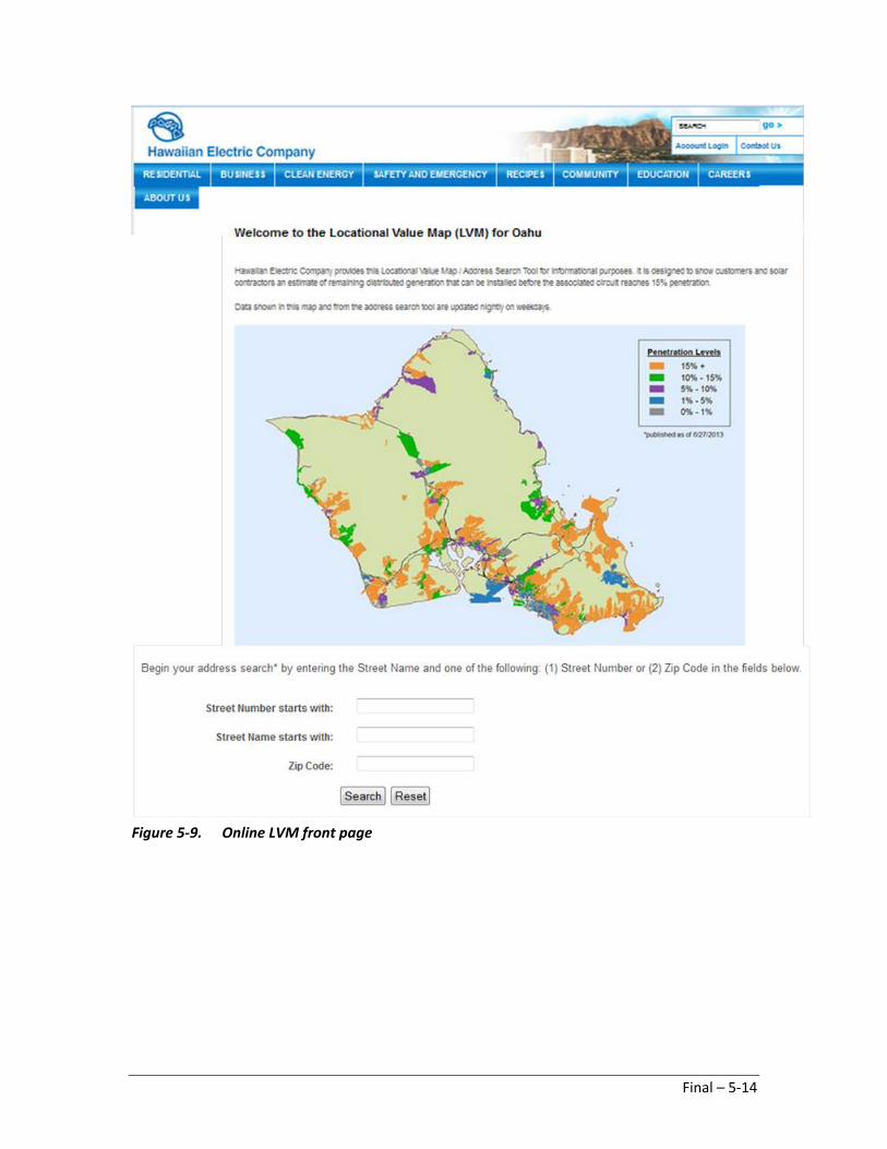
Figure 5-9. Online LVM front page

Final – 5-14

Figure 5-10. Sample online address query display results

Efforts are underway to continuously improve the internal GIS-based LVM tools and the Online LVM to support better communication of information to the public. Due to recent exponential growth in PV, additional percentage levels above the 15% penetration have been added to the Online LVM to better inform developers and customers where supplemental reviews are likely to be needed. Figures 5-11a, b, and c provide views of the new 5-tone LVM for tracking percent penetration levels through 100% of circuit maximums and circuit daytime minimum gross load (load + PV generated load). Because so many of the island feeders are already beyond 15% of maximum PV penetration, customers and developers desired better guidance on penetration on feeders beyond 15% and up to levels that would likely require further review through interconnection studies.

Final – 5-15

(a)

(b)

Final – 5-16

(c) Figure 5-11. New 5-tone LVM with (a) percentage penetration of circuit maximum,

(b) percentage penetration by circuit daytime minimum load and (c) all island summary (source: HECO)

5.2.3 REWatch

The Renewable Watch was developed to provide utility staff and customers with visibility as to the value of renewable resources during various times of the day. One of the biggest challenges for utilities contending with high penetrations of PV, especially behind-the-meter, is the lack of visibility to the amount of energy being generated by local distributed systems. Many utility staff and customers are not aware of the variability impacts of PV on the grid, how rapidly conditions change with cloud cover, how much renewable generation is available, and when they are generating during the course of the day.

Figure 5-12 shows the current Renewable Watch contents page. Featured windows include the following:

• ‘Renewable Watch – Today’ window which updates system information every 15 minutes

• ‘Renewable Production’ information by aggregated regions shown in a tabular format

• ‘Renewable Watch-Yesterday’ window showing system information for the prior day conditions in comparison to current day

Final – 5-17

• Weather forecast information on the lower left

• ‘Information’ window with brief explanation of the data shown

Figure 5-12. Renewable Watch for Oahu

5.2.4 Operations Integration

The Operations Integration effort focuses on getting Operator’s access and using renewable and DG information for decision making by enhancing the EMS environment.

This visualization effort leverages the DG aggregation and modeling efforts conducted as part of Task 2 of the SMUD/HECO High Penetration PV Initiative and Task 3 solar monitoring for improving renewable energy forecasting with AWS TruePower, a leading U.S. based renewable energy forecasting provider. Figure 5-13 provides a conceptual view of the information flow and enhancements to be derived in the enhanced EMS environment.

Final – 5-18

Figure 5-13. Conceptual view of new data and EMS environment enhancements

New logic is being investigated and prototyped by EMS providers to the Hawaiian utilities (Alstom and Siemens) to account for DG and non-DG resources on the grid and to incorporate real-time probabilistic forecasts (Figure 5-14). Efforts focus on the following:

• Develop and test out an aggregation approach for integrating the distributed PV installations and information for system operations

• Develop and test new EMS logic to use new forecasting data streams, confidence bands and ramp statistics

• Develop functional prototypes or mock-up displays and alert capability to inform real-time operations of changing renewable conditions

• Test out CIM format to update DG field information and distribution network needs

• Involve and gather operator feedback on the design, use and evaluation

Efforts also require close interaction with System Operations Network and ITS support personnel to ensure development of a sustainable and cyber-secure process for updating the DG data and accessing real-time renewable forecasts from renewable energy forecast providers. With increasing levels of variable generation and distributed behind-the-meter generation, these resources cannot be ignored and will have impacts on system operation, especially during contingency events.

Final – 5-19

This task will continue under the recently funded U.S. Department of Energy Sunshot program to continue and engage control room operators for feedback and participation throughout the development and integration process. Each EMS vendor will work with the end-use utilities to accomplish the following:

• Create more accurate assessments of VER/DER in current state and near-future situations

• Develop configurable visuals and multi-level alerts to help system operators monitor and inform action

• Prototype platform showcasing capabilities and gather user feedback on benefits and use

• Provide recommendations on standardizing utility data transfer Common Information Model (CIM) protocol, training and application strategies

Final – 5-20

Figure 5-14. Prototype of regional forecasts and ramp statistics (source: Siemens and HECO)

Final – 5-21

5.3 Outcomes

Over 2 years, HECO in partnership with SMUD has deployed and successfully piloted new visualization and field monitoring technologies (such as the TREX, location value maps, and the renewable energy watch maps) to gain better understanding and visibility to the increasing levels of distributed PV on the grid. Visualization efforts leveraged other tasks conducted as part of the HiP-PV Initiative, including modeling, monitoring, forecasting, and technical outreach. Utility efforts were also conducted in partnership with industry and vendor providers looking to improve their products through better integration and user feedback.

Desired outcomes from the effort included:

• Improve management of PV variability and unit commitment with new field information

• Reduce utility costs (reserves, heat rate, curtailments) and improve the customer experience

• Inform vendors partnerships to help address needs

• Engage and build workforce with confidence to change

The work resulted in the design and development of new data management architecture to support real-time operations and planning. Efforts also helped develop insight on training needs, engaging existing workforce and developing future workforce skillsets. Visualization tools deployed and lessons learned will help utilities build expertise in managing variable DG resources while preserving for locational benefits and accounting for impacts.

5.4 Lessons Learned

Lessons learned include the following:

1. Technology:

A. Utility tools from data processing, data management, analytics, and visualization must be improved, in order to manage the increasing and diverse variable resources.

B. New secure architecture for bi-directional exchange of data needs management direction and attention (outsource or support with house capabilities).

2. Operational Process:

A. The shift toward real-time, heads-up, and dynamic dispatch and load management requires the convergence of tools, resources and multi-disciplinary expertise.

B. System management during emergency and contingency events can benefit with higher fidelity data, advance real-time forecasting, and a heads-up, but daily operations and dispatch can also be significantly improved and optimized with similar information if they can be incorporated into real-time operational tools.

Final – 5-22

3. People/Communication:

A. Engage and involve existing vendor partnerships and commitment to provide product-based solutions.

B. Update decision makers often, but prototype and test with user group.

Visualization tools provided a number of benefits, but the experience gained in developing an approach, engaging the workforce, introducing new process, and implementing the technology provided valuable insight to help utilities transform. Experience gained in deploying instrumentation, data analysis, and lessons learned in the results of this project have provided benefits to HECO and SMUD and can directly apply to other utilities as their PV penetration levels increase and as they consider monitoring options. Benefits include:

• Real-time information to help utilities better see impact of renewables and integrate information into planning and operations

• Transparency to the public

• Increase awareness by workforce on value of renewables

• Sharing of integration experience through industry forums and utility venues

• Continuing collaboration to seek internal and federal funding

• Improve management of PV variability and unit commitment with new field information

• Engage and build workforce and vendor confidence to change

• Secure, reusable interfaces for data exchange and integration of DG and forecasting data into the EMS environment.

• Addressed people, process, and technology enhancements

– CSI-funded effort helped small utilities like HECO and SMUD address high penetration needs and was one of the first efforts to focus awareness of distributed energy resource impacts on systems

– Efforts provided impetus for industry (EMS, forecasting, model providers, standards, regulatory, and other utilities) to partner and focus on integrated solutions

– Funds jumpstarted lasting initiatives that are being adopted into HECO company processes and regulatory recommendations (interconnection standards, Reliability Standards Working Group)

• Resulted in numerous technical presentations and papers (Institute of Electrical and Electronics Engineers [IEEE], American Wind Energy Association, Solar Electric Power Association, Distributech, EPRI, CPUC/DOE] joint meetings) throughout project period to inform market product development and industry standards development

Final – 5-23

Efforts are leaving a lasting impact by:

• Encouraging utility/vendor partnering to further develop and operationalize visualization tools (EMS, forecasting, online tools)

• Supporting ongoing collaborations on proposals for industry and federal funding (FOA, laboratory and training center) to further develop and implement technologies

• Inform standards development (Federal Energy Regulatory Commission, North American Electric Reliability Corporation, IEEE, Underwriters Laboratories) related to DG and forecasting needs

• Contributing new insights to regulatory proceeding and new utility process development

Working with a team of industry partners including Siemens, Alstom, AWS Truepower, DNV, Referentia Systems Inc., and various sensors and telecom providers, new visualization and analytical tools were developed with utility feedback, jointly piloted in the field, transitioned into implementation, and are now being utilized to help manage very high penetrations of variable DG. Utility partnership in enhancing vendor products has also been positively received by the partners on this team. Building on the results of the CSI funding, this same project team was recently awarded a U.S. Department of Energy (DOE) Sunshot grant to continue implementation efforts and integrate the forecasting data, aggregated DG modeling tools, and field data into System Operation’s EMS decision tools. Siemens and Alstom EMS tools are used by Hawaiian utilities and a number of western utilities including California IOUs and the California Independent System Operator (California ISO).

The development and deployment of a robust architecture to support renewable integration and data management needs will continue to evolve with new technologies. However without a common platform to centralize information and conduct such analysis, it will be increasingly difficult to manage large volumes of renewable information and to effectively utilize grid intelligence from customers (AMI) to inform future automation needs and optimize use of new technologies such as faster demand response (FastDR) and customer options.

The new visualizations are being expanded to provide information to customers and support communications of renewable development to customers and policy makers.

Final – 5-24

6.0 SOLAR MONITORING AND PV PRODUCTION FORECASTING

Note: Information in this section was excerpted from High Penetration PV Initiative: PV Monitoring and Production Forecasting (http://calsolarresearch.ca.gov/images/stories/ documents/Sol1_funded_proj_docs/SMUD/SMUD-NEO_HiPenPV_FinalRpt_2013.pdf).

6.1 Objectives

The overall objective of this solar monitoring and PV production and forecasting work performed by NEO under this grant was to complement that of the other team members and to share a vision of the future of utility solar forecasting as a fundamental component of grid management for enhanced stability and optimized economic performance. In that shared vision distributed solar monitoring and forecasting of PV production will move out of the realm of research and into the utility control room as a standard component of EMS/SCADA (HECO visualization systems) and providing monitoring of energy flow at the feeder level (DNV GL) and inform utilities and ISOs with actionable data for dispatch, demand response, energy storage, inverter VAR control or curtailment (SMUD)

The IOUs in California can leverage much of the work presented in this report immediately by applying it to their own needs for management of increasing levels of PV on their distribution networks. IOUs can use forecasts in the day-ahead time frame to inform unit commitment and as an input to day-ahead energy trading decisions. As the IOUs deploy more smart grid technologies, the day-ahead and near-term forecasting methods described in this report can provide inputs to their control algorithms. For those utilities that are already invested in PV forecast technologies such as satellite and sky camera services, this report illustrates the way in which real time ground truth irradiance measurements across their service territories can serve as references or corrections to the data streams coming from those systems. For those IOUs that have not yet invested in solar power forecasting services or technologies, duplicating part of the work performed in this study IOUs can leverage their own solar resource measurement capabilities to validate the claims of solar forecast vendors and help select products and services suitable for their operations.

This task included the following objectives:

• Forecast regional irradiance for a day-ahead window 20 to 36 hours in the future

• Model PV production for regional PV installations based on the day-ahead forecast

• Validate the day-ahead forecast irradiance and PV production data with measured data

• Forecast regional irradiance for a short-term window 1 to 3 hours in the future

• Model PV production for regional PV installations based on the short-term forecast

Final – 6-1

• Validate the 1 to 3 hours forecast irradiance and PV production data with measured data

• Merge SMUD feeder load and PV forecast data

6.2 Approach

NEO was responsible for this task, including the design, fabrication, deployment 3, and maintenance of an irradiance monitoring network. The network was designed to collect 1 year of global horizontal irradiance (GHI) and ambient temperature in SMUD’s service territory. NEO was further tasked with creating and maintaining a database of the collected data and making it accessible to SMUD.

The original scope of work for this subtask was intended as a roadmap for obtaining the short-term (0-3 hour) and long-term (day-ahead) solar forecasting and validation goals of this project. That roadmap laid out one possible path to achieving these goals. Most, but not all of this path was followed as developments and discoveries presented themselves through the course of the project.

6.2.1 Design, Manufacture, Deploy and Maintain 5 km Irradiance Monitoring Network

6.2.1.1 Creating the Monitoring Network

This effort consisted of a range of technical and logistical subtasks required to design, manufacture and deploy a monitoring network of five primary and 66 lower cost secondary irradiance monitoring stations. The network was deployed on a 5 km grid using autonomous PV/battery powered data loggers installed in substations and on SMUD utility poles. The five primary stations used rotating shadowband radiometers (RSRs) to collect and store irradiance measurements at the substations, while independent data loggers combined with global horizontal pyranometers made up the 66 secondary monitoring stations (Figure 6-1 and Figure 6-2).

3 NEO Virtus Engineering and SMUD collaborated on the identification and mapping of the installation sites. NEO coordinated the installations with SMUD line crews performing the actual installations on utility poles. SMUD's data technician and NEO personnel performed the installations of the five primary stations.

Final – 6-2

Figure 6-1. Primary station (rotating shadowband radiometer) located on roof of

California State University Sacramento

The primary RSR stations required almost no modification because the RSR is an existing commercial product NEO manufactures for its client, Irradiance, Inc. The secondary stations, however, were designed from scratch for this project due to the unique requirement for mounting on utility poles. The exterior enclosure design includes a PV module and bracket, an adjustable pyranometer arm, and support bracket for easy pole mount. The internal enclosure design houses a battery, data logger, cellular modem, and associated electronics. Both the primary and secondary stations use Licor 200SZ silicon pyranometers for irradiance measurements. The secondary station enclosure and the internal mounting armature are entirely non-metallic, allowing the modem antenna to be mounted internally.

Final – 6-3

Figure 6-2. Fabrication of the secondary stations at NEO Virtus Engineering, Inc.

Sheet metal and non-metallic parts were machined and the secondary units were assembled, programmed, and tested at NEO's Littleton, Massachusetts, facility (Figure 6-2). The calibration of each pyranometer was checked by comparing its output with that of the others in sets of 25 under identical irradiance conditions. Bulk rate cellular data plans were negotiated based upon data transmission bit calculations. Two prototype units were deployed, one pole mount and one on SMUD’s headquarters roof, to assure cellular connectivity and to collect sample data sets. Each of the secondary station production units was bench tested then field tested on NEO’s roof in its final assembled form before shipping. Units were shipped in batches of 16 to SMUD’s Sacramento warehouse where, once received, they became property of SMUD.

SMUD’s GIS department overlaid a map of available assets (locations for mounting primary and secondary monitoring stations such as utility poles, buildings, and secure land) onto the NDFD forecast 5 km grid. The approximate centroid of each NDFD grid cell was targeted. SMUD staff surveyed the candidate sites and coordinated with SMUD’s line crews for approval of final locations. Installation of secondary monitoring stations started in early April and was completed in late May. After each installation (Figure 6-3), prior to the line crew leaving the site, the foreman called in the completed installation to NEO for confirmation of cellular connectivity.

Final – 6-4

Figure 6-3. SMUD lineman installing one of the secondary stations in Sacramento, California

All 66 of the secondary stations were mounted on utility poles. Four of the primary stations were installed on tripods. Two of the RSR tripods had to have extensions to raise the measurement device above shading obstructions. Even after elevating the RSRs, some experienced early morning and late afternoon shading, especially in the winter months. Figure 6-4 shows the locations of the sensors in the network in SMUD’s service territory.

Final – 6-5

Figure 6-4. SMUD-NEO irradiance network

Data Collection

Data (irradiance and ambient temperature) is collected by connecting to each station’s cellular modem. The cellular modems are programmed to turn on for 1 hour during the night to conserve battery power. During this nightly window, Campbell Scientific Loggernet Admin software is set up to call each station, attempt connection, and if cellular connection can be made, collect data. The collection window was set up for the middle of the night, because cellular traffic is lower during this period, so the chance of connection will be greater. Should the connection fail, a second window during the day was also set up to attempt a second automatic collection. Manual collections can also be attempted during this period. Upon successful data collection, the raw data files are saved on a dedicated RAID server and are automatically pushed into a MySQL database using Loggernet Database software. NEO also maintains a redundant computer running Loggernet which connects and collects data as a backup.

Maintenance of Network

In general, the network has required very little maintenance. The RSR units collected and reported daily nearly without any gaps. The secondary stations, for the most part, also collected and reported automatically as programmed. There were, however, occasional glitches or

Final – 6-6

equipment failures that required action. Also, though generally very strong, cellular coverage for some sites was sometimes intermittent. At the end of the extended 24-month monitoring period, the data set was 98.5% complete and the mean time between failure was 10.1 years.

Each weekday the previous night's collection was checked for units which failed to respond. Those that did not were called and a second attempt was made to collect data during the day. Units which did not collect were logged in a tracking spreadsheet and checked the following day. The secondary station data loggers had approximately a month of data storage capacity before they began to lose data. If a unit failed to collect long enough, SMUD was informed and the unit was replaced. NEO developed tools that allowed us to view multiple sensor signals simultaneously and provide a quick visual inspection, as seen in Figure 6-5.

Figure 6-5. Loggernet RTMC data monitoring window; secondary sensors 12 to 22

In addition to monitoring the irradiance signals, each system's reported daily battery voltage minima and maxima were monitored. Data windows were created using the Campbell Scientific data logger's real-time monitor and control (RTMC) application, as shown in Figure 6-6, that allowed our staff to view the status of all 66 secondary station batteries at a glance. identified batteries that were beginning to discharge to unsafe levels and their cellular calling windows could be modified to reduce daily load.

Final – 6-7

Figure 6-6. Battery state of charge view screen; 66 stations

The most serious problem encountered during the first year was a software issue related to the data loggers installed in each unit (Campbell Scientific CR200). Three secondary units stopped recording data in February 2012. Troubleshooting determined there was a failure in the flash memory of their data loggers due to too many “writes” to a certain section of the memory. A programming fix was worked out with Campbell Scientific, and all secondary stations received a program update. NEO reprogrammed 54 secondary stations remotely and 12 units were reprogrammed/repaired/replaced in the field, completing the fix for the flash memory issue. Campbell Scientific provided warranty replacement for four failed data loggers.

Other field failures included two units with pyranometer arms that had slipped below horizontal (fixed on site), one unit with a defective solar panel junction box, and one unit with a defective data logger. Occasionally a unit would stop communicating with the Loggernet program, but this was always found to be an issue with local cellular service (i.e., the modem in the unit could not be dialed up because of poor reception or network outage).

To ensure maximum integrity of the network, NEO built two spare secondary units in late 2011. One unit was always maintained at NEO’s offices, while the second unit was kept at SMUD’s Headquarter as a hot spare, ready to be utilized when needed. A customized, hard-sided shipping case (pelican case) was procured to protect the units during shipment. This

Final – 6-8

replacement system set up minimized down-time for any particular network node and also maximized the chances of a unit arriving safely at its destination.

6.2.1.2 Data Quality Management

Early in the monitoring process anomalies in the data were found. During portions of the year when the solar zenith angle is relatively small (i.e., when the sun is high in the sky), the overhead wires and cross arms briefly cast shadows on the pyranometer. These shadow events present as very discrete and repeatable anomalies on clear sky days. Figure 6-7 has two images of global irradiance and temperature measured by unit 64 on 2 clear sky days 2 weeks apart where characteristic shading events of the same magnitude occur at the same times of day. These shading anomalies, when viewed on clear sky days, represent a kind of signature for the monitoring unit in its unique location.

Figure 6-7. Irradiance signals on 2 clear days, 2 weeks apart

Researchers at SMUD and Sandia developed a method to filter the data set for these recurring anomalies. The anomalous values were identified and the data were interpolated between the first and last good data point in the series (Bing, J., Bartholomy, O., Sison-Lebrilla, E., Thomas, W., Vargas, T., Williams, R., SMUD-NEO Irradiance (SNI) Network Open Access Database, American Solar Energy Society, 2013). NEO used the cleaned, interpolated data for forecast validation. Both the raw and cleaned, interpolated data are available for public use on SMUD's website at ftp://ftp01.smud.org/pub/SNIData/.

One practical limitation of the secondary sensor network is that the sensors are widely distributed and require a bucket truck to access. Thus, they would have been extremely difficult to keep clean using a typical 2-week schedule. A small set of higher accuracy sensors were added to measure irradiance independently of the network to help verify the calibration of the installed pyranometers and hence the quality of overall network irradiance data. Three of the four locations are in substation yards and one is on the roof of a five-story building. We had

0

5

10

15

20

25

30

35

0

100

200

300

400

500

600

700

800

900

1000

1100

5:30 6:30 7:30 8:30 9:30 10:30 11:30 12:30 13:30 14:30 15:30 16:30 17:30 18:30 19:30 20:30

Tem

pera

ture

(°C)

Irra

dian

ce (W

/m2 )

Time (Pacific Standard Time)

Global Horizontal Radiation 6/25/11 SMUD/NEO Virtus Secondary Station #64

DAS# 64 POLE# UD122802 LAT: 38.59662 LON: -121.48561 Temp (⁰C)

0

5

10

15

20

25

30

35

0

100

200

300

400

500

600

700

800

900

1000

1100

5:30 6:30 7:30 8:30 9:30 10:30 11:30 12:30 13:30 14:30 15:30 16:30 17:30 18:30 19:30 20:30

Tem

pera

ture

(°C)

Irra

dian

ce (W

/m2 )

Time (Pacific Standard Time)

Global Horizontal Radiation 07/09/11 SMUD/NEO Virtus Secondary Station #64

DAS# 64 POLE# UD122802 LAT: 38.59662 LON: -121.48561 Temp (⁰C)

Final – 6-9

some concern regarding dust in the substations; however, the devices were scheduled for cleaning every other week so we concluded soiling would not be an issue.

These additional irradiance sensors were installed at four of the primary stations. Their data were incorporated into the database as part of a calibration plan for the network, and also into the distribution of daily updates of the data set. For the four sites in question, Eppley Laboratory’s Precision Spectral Pyranometers (PSP), as seen in Figure 6-8, were installed in global horizontal orientation and their signals added to the data stream. NEO provided two PSPs and SMUD provided two PSPs, all of which were calibrated at NREL using their Broadband Outdoor Radiometer Calibration (BORCAL) procedure prior to deployment.

Figure 6-8. One of the four RSRs with a PSP installed

These four PSPs are distributed around SMUD’s service territory, approximately at the compass points (Figure 6-9). The four RSR locations with PSPs are Anatolia, Don Julio, and Twin Cities substations and on the roof of CSUS. Note that the RSR at Anatolia substation was deployed by NREL at an earlier date. NEO accesses the data from Anatolia via NREL’s website. The four PSPs are maintained with an approximate 2-week cleaning schedule.

Final – 6-10

Figure 6-9. Locations of four Eppley Precision Spectral Pyranometers

6.2.1.3 Additional Scope of Work

During the course of this project lessons were learned which had not originally been anticipated. The four PSPs used to provide global calibration of the network are just one such example which, once we'd deployed the network, made sense to do and thus became an addition to our original scope.

Another development which had not been anticipated in the original proposal was the need by SMUD for enhanced power systems on three of the five primary stations. For three of the four primary units installed in SMUD substations, 110 watt PV power system (factory default is 20 watt) were provided for a SMUD spread spectrum modem that ran 24 hours per day7 days per week and which delivered RSR data to SMUD substation SCADA. The RSR on the roof of CSUS was provided with an AC power system and a direct Ethernet connection to CSUS’s LAN. This added connectivity provided a backup data path in case the cellular modem failed.

Another modification not anticipated by the original proposal was the programming necessary for daily network data uploads on a site-by-site basis. The first 3 months of collected data were transmitted to SMUD in the fall of 2011, and then sent a data set including the first 6 months of

PSP1 at Don Julio substation

PSP1 at CSUS

PSP1 at Anatolia substation

Circles indicate sensor nodes

PSP1 at Twin Cities substation

Final – 6-11

data in late 2011. However, handling the data in such large sets was somewhat difficult, and did not give SMUD engineers access to collected data in a timely fashion. A method was devised so that SMUD would be able to access the collected data in near real time. NEO transmitted the data to SMUD via daily ftp upload, using Campbell Baler software to parse the large raw data files into 24-hour chunks that are automatically uploaded to the SMUD ftp site using WinSCP software.

In June of 2012, delivery of daily forecasts of FIT system power production began, providing hourly forecasts of plant production in a window 22 to 40 hours into the future, delivering the data at about 5:20 a.m. Pacific local time for Bruceville, Kost, Boessow, and Point Pleasant. Due to SMUD information technology security concerns, the forecasts were delivered as email attachments rather than other, more direct methods, such as writing directly to their server.

Other methods of data delivery and end user access were evaluated to make these forecast services more widely available, flexible, and user friendly. The possibility of designing a scalable online solution with cloud based computing and data storage (presently all programs run on NEO server) were also evaluated. A Beta version of a graphical user interface (Figure 6-10) that would provide end users with the ability to selectively access forecasts of irradiance and plant production for specific ranges of dates in the future, daily time frames, and locations was also created. The tool would provide both numeric file and graphical reporting options.

Figure 6-10. NEO solar forecast graphical user interface

Final – 6-12

6.2.1.4 Summary

NEO designed and built the required 66 secondary stations, assembled the five primary stations (RSRs), and shipped all 71 units to Sacramento, where over the course of several weeks, they were all installed by SMUD linemen. NEO also developed an automated data retrieval system, created a MySQL database to store the collected data, and uploaded daily updates of the data to SMUD’s ftp site.

This network has been up and running since June 2011. A total of 24 months of data were collected as of June of 2013. Irradiance data from four PSPs was collected and used to help verify the calibration of the network sensors.

SMUD plans to maintain the monitoring network for an additional 2 years with NEO providing the sensor maintenance and data collection. The data will be used in a DOE grant-funded project with the University Corporation for Atmospheric Research. The resulting data set continues to be of value for validation of a range of forecasting technologies from numerical weather prediction models, to satellite imagery, to sky camera approaches. SMUD has used parts of the network for validation of battery dispatch in the community. Further SMUD is using the data set in an evaluation of trials of a number of different solar forecast products. Finally as a sub-recipient of the National Center for Atmospheric Research's grant under the DOE FOA-0000649, "Improving the Accuracy of Solar Forecasting," SMUD is providing ground truth irradiance data from the network for improving accuracy of solar forecasting in the short-term (0-6 hours) and day-ahead timeframes.

Looking ahead, the future use of the secondary sensors has many possibilities. Of the five analog inputs on the CR200 data logger only two are presently in use, meaning that the units could be repurposed for a wide range of applications in solar resource assessment or other fields.

6.2.2 Develop 20-36 Hour Feed-Forward PV Forecasting Model

The objectives of this task were to forecast regional irradiance and PV production of SMUD’s FIT PV power plants 20 to 36 hours in the future, i.e., one day ahead. Such forecasts could provide information for making generation resource scheduling and purchase and sales decisions in the next-day energy market. The production data from the FIT sites and the installed sensor network provided measured power and irradiance data needed to evaluate the model’s performance. This task was broken into several steps, including development of the irradiance transmittance model, an irradiance surface model, a photovoltaic generation model, and the integration of all of these into a 20-36 hour-ahead PV production forecast model to calculate FIT plant power output. All of these steps were preceded by the creation of relational database developed to store the fetched NDFD meteorological forecast data. That same relational database became the home for the FIT site parameters, the inverter parameters, and the Sandia PV module database used by the forecast model.

Final – 6-13

6.2.2.1 REST2 Transmittance Model

The goal was to use the National Weather Service's NDFD meteorological forecasts to predict the solar irradiance incident on various PV systems from 20 to 36 hours after forecast issuance. NEO contracted with Solar Consulting Services (SCS) for this task. SCS’ work was accomplished by Dr. Chris Gueymard, a well-known expert in this field. For this task, he used his high-performance Reference Evaluation of Solar Transmittance 2 bands (REST2) clear-sky radiation model (Gueymard, 2008) and made various modifications, additions and improvements, as described below. REST2 calculates clear-sky radiation from site coordinates and atmospheric data.

A study was made to obtain the mean daily values of the required aerosol parameters. These were derived from satellite data, after bias correction using available ground observations in the general area. At this point, there are no reliable forecasts of hourly aerosol optical depth variables at a sufficiently high spatial resolution, but this should not be a big issue over Sacramento.

Another study was conducted to evaluate the water vapor concentration of the atmosphere (in terms of precipitable water, PW). Three local GPS stations of the National Oceanic and Atmospheric Administration (NOAA) network were used: Lincoln, McClellan AFB, and Dixon. A statistical relationship was found between the measured PW and the measured vapor pressure, itself derived from temperature and relative humidity through well-established physical equations. The latter two quantities are provided by NDFD, and can therefore be used to derive the necessary PW forecasts.

Reasonable monthly values of the other necessary inputs to REST2 (ozone, nitrogen dioxide, and surface albedo) were determined. A validation exercise to evaluate the performance of the hourly irradiance predictions was conducted at Anatolia and showed good results.

The main study was devoted to relating the NDFD cloud fraction forecasts (at unfortunately a low temporal resolution—only a 6-hour refresh rate) to the cloud attenuation evaluated at the Anatolia RSR station by dividing the observed GHI and DNI by the calculated clear-sky values. Cloud transmittance functions were obtained for various classes of cloud fraction and solar position, with or without precipitation. It was observed that the forecasts of fog or marine layer were not correct, unfortunately (out of phase or simply missing). The evaluation of DNI under cloudy conditions was improved through an optimal combination of (i) the prediction derived by modifying the ideal clear-sky value by a cloud transmittance function; and (ii) an independent prediction based on the popular Erbs correlation that provides the diffuse/global ratio through statistical means (Erbs et al., 1982). Compared to the good results of the clear-sky predictions, the cloudy-sky situations showed large random errors, which can be explained by the insufficient refresh rate (6 hours) of the cloud forecasts, the inaccuracy of the forecasted cloud fraction under many circumstances (e.g., fog and marine layer), and the lack of additional information about layer-by-layer cloud type or cloud optical depth.

Final – 6-14

A similar study was conducted to derive the necessary cloud cover correction factor, using a similar approach, to provide day-ahead GHI, DNI and global tilted irradiance (GTI) forecasts close to the Honolulu area. Measured irradiance data from NREL’s RSR station at Honolulu’s airport were used to calibrate the model. Even more difficulty with the NDFD cloud forecasts was found there, compared to Sacramento. It is probable that the coastal location of the station, and that the typical local cloud regime (scattered cumulus clouds) adds to the difficulty.

6.2.2.2 PV Surface Irradiance Model

An algorithm (Gueymard, 1987) was added to the one previously described so that the GTI—also referred to as plane-of-array irradiance or PV surface irradiance—could be evaluated (modeled) each hour. This algorithm is normally applied to the most frequent case of fixed-tilt PV systems. A modification was introduced to make it also accept the case of single-axis tracking systems, with or without backtracking.

6.2.2.3 Photovoltaic Generation Model Integration

NEO's approach to calculating PV plant output power was accomplished by creating three main program components:

1. The main program

2. An executable version of the REST2 transmittance model code

3. The relational database with all relevant system data

Main Program

The main program, DAE_analyze.pl, performs all of the calling functions and runs the Sandia Photovoltaic Array Model. DAE_analyze also calls the compiled executable version of REST2 and hands it the forecast meteorological data and PV plant data it needs to return a value of GTI. In addition DAE_analyze provides all of the routines that fetch, parse, and store to the database the necessary forecast meteorological data from the NDFD.

REST2 Executable

The REST2 transmittance model and the PV surface irradiance models were written in Fortran and then compiled to an executable form by Bruce McArdle. When run, the executable version of REST2 calculates the direct normal, diffuse horizontal, and global horizontal components of irradiance at the specified latitude and longitude based upon the forecast meteorological parameters it has been given. Those general forecast values of irradiance are then translated by REST2 into values of global tilt irradiance. Global tilt irradiance is the irradiance incident upon a specific array module surface, whether it is a fixed tilt or tracking surface. The program also calculates the effect of near field shading and array self shading.

Final – 6-15

Relational Database

The open source MySQL relational database was chosen for this project based on its capabilities and cost. The MySQL database serves as the repository for the Sandia Module database, NEO's inverter database and the database of SMUD FIT system characteristics. The database was first used to store the meteorological parameters used by the transmittance model, REST2, retrieved from the NDFD. Principal amongst these parameters are sky cover, temperature, and probability of precipitation. The Sandia Module database is a listing of some of the thousands of commercially available PV modules that have been tested and characterized by Sandia. NEO's inverter database contains a list of inverters used at the SMUD FIT sites with DC/AC conversion efficiencies expressed as a function of percentage of full load. The MySQL database also contains a table listing site data for all of the SMUD FIT PV plants. The parameters include site latitude, longitude, elevation, module and inverter make and model, array tilt, azimuth and tracking/no tracking status.

6.2.2.4 20-36 Hour Feed-Forward PV Forecasting Model Integration

Each of the sub-models and the MySQL database functions described above were developed and tested independently and then, in some cases, tested together in a piece-wise fashion. To better understand the Sandia PV Array Model, NEO consultant Robert Williams coded it in a Microsoft Excel spreadsheet and ran it a step at a time. However before the entire process could be run end to end using its separate components, the main routine, DAE_analyze, was completed and the process naturally transitioned to full automation. The full process starts with DAE_fetch retrieving the forecast met data from NDFD, decoding those data from their gridded binary format to a csv format, filtering the data for the geographic subset of sites included in the sensor network, and then pushing the forecast data into MySQL. Next the program calls the REST2 executable, queries the database for forecast met data, site data, module and inverter data. Once the REST2 transmittance model has delivered a value of GTI, the program calculates the instantaneous power based upon a 1-hour time increment, then pushes this to the database.

One of the challenges associated with this project was the proliferation of reference times. The end user, the SMUD energy trading department, operates in local Pacific time. This of course means that they use daylight saving time when it applies. All of the NDFD references were to Greenwich Mean Time. REST2 uses local (Pacific) standard time throughout the year. The calculation done in NEO's Massachusetts office occurred at Eastern time, with daylight saving time and a 3 hour difference from the end user in California.

The original intent had been to do all of the day-ahead, 20-36 hour forecasting, in a post processing hind cast mode. In this mode, historical NDFD forecasts would be retrieved from the National Climactic Data Center and those data would then be used to generate historical forecasts that would then be tested against historical FIT PV plant production data and against the historical measured data global horizontal irradiance date from the SMUD-NEO sensor network.

Final – 6-16

However as the end of 2011 approached and several of SMUD's FIT sites neared completion, NEO was asked to provide a Beta version of the real time forecast. We were told that there was a need in SMUD's energy trading department for a forecast of the next day's contribution by the FIT sites. On June 5, 2012, NEO began sending forecast of the production for Bruceville, Kost, Boessow, and Point Pleasant, a total capacity of 30 MW capacity to SMUD. SMUD's energy trading schedule required that they receive the forecast at 5:00 a.m. Pacific time. To accommodate this schedule we adjusted our forecast window to 22 to 40 hours into the future. The final forecasts of this project, which were done for the purposes of model performance validation, were done as hindcast calculations using the 22-40 hour forecast window and the latest improvements to the component models. The time frame for the validation set of forecasts was from May 1, 2012, to April 30, 2013. Figure 6-11 illustrates 3 days comparing forecast and measured production at two of the FIT sites. Note that hours of darkness have been eliminated, since predicting night output is unnecessary.

Final – 6-17

Figure 6-11. Sample from two sites, comparing forecast and measured production

on mostly clear days

The forecasts on the sample days, most of which were clear days, performed reasonably well with the exception of May 17 and May 19 when the model underestimated the measured power.

0.0

0.5

1.0

1.5

2.0

2.5

3.0

3.5

6:00

:00

8:00

:00

10:0

0:00

12:0

0:00

14:0

0:00

16:0

0:00

18:0

0:00

6:00

:00

8:00

:00

10:0

0:00

12:0

0:00

14:0

0:00

16:0

0:00

18:0

0:00

6:00

:00

8:00

:00

10:0

0:00

12:0

0:00

14:0

0:00

16:0

0:00

18:0

0:00

MW

Kost (3MW): 5/17 - 5/19, 2012

Forecast power Measured Power

0.02.04.06.08.0

10.012.014.016.018.020.0

6:00

:00

8:00

:00

10:0

0:00

12:0

0:00

14:0

0:00

16:0

0:00

18:0

0:00

6:00

:00

8:00

:00

10:0

0:00

12:0

0:00

14:0

0:00

16:0

0:00

18:0

0:00

6:00

:00

8:00

:00

10:0

0:00

12:0

0:00

14:0

0:00

16:0

0:00

18:0

0:00

MW

Bruceville (15MW): 5/18 - 5/20 2012

Forecast power Measured Power

Final – 6-18

6.2.2.5 Summary

NEO and its consultants successfully implemented the irradiance and PV power production forecast methodology described in the project scope of work. Our efforts resulted in PV production forecasts in the day-ahead time frame which have been delivered to SMUD on a daily basis since the beginning of June 2012.

6.2.3 Develop 0-3 Hour Feed-Forward PV Forecasting Model

The objective of this subtask was to forecast regional irradiance and PV production of SMUD’s FIT PV power plants 1-3 hours out, i.e., in the short term, using the global horizontal data from the sensing network. Note: The time frame was initially described as a 1-3 hour forecast in order to describe the time period in the first hour ahead and the first 3 hours ahead. Because this was the source of some confusion, we changed the subtask to a 0-3 hour forecast (henceforth referred to here as 0-3 hour.)

6.2.3.1 Develop 0-3 Hour Feed-Forward PV Forecasting

Ground Level Irradiance Velocity Vector Recognition

The approach to short-term sensor-based irradiance forecasting we proposed in the initial scope of work was one in which we would use all of the measured irradiance data from the monitoring network at the same time. The basic concept for forecasting irradiance based upon ground sensor measurements was one of pattern recognition similar to that described in Bosch et al under the concept name, Most Correlated Pair, but with the benefit of a much larger array of sensors. The process entails synthesizing an image of irradiance levels at an instant in time comprised of GHI levels measured by our network of sensors. This irradiance image would be like an image created by a black and white digital camera using a charge coupled device (CCD) where each value of irradiance reported from the sensor network is similar to a light level in a pixel of a CCD element. As illustrated in Figure 6-12, the first image, I, at time t1 (It1) in a daily cycle is taken shortly after sunrise because this process is only run during the daylight hours. At some time after It1, for example 1 minute, which is the equivalent of one record, the program would synthesize a second image, It2, from global horizontal irradiance levels measured by our network. After synthesizing It2, the program would then compare It1 to It2. Using an approach similar to the “Most Correlated Pair” method, we would derive a velocity vector that represents the displacement in time and distance between It1 and It2. Using the synthesized irradiance image It2, in combination with the image velocity vector, it would then forecast a future irradiance image by estimating the location of irradiance image It2, at time t3. This forecast irradiance image, FIt3, is the result we are seeking. This forecast image of irradiance will be transformed into a forecast of AC power generated by solar PV systems in the area of the sensor network.

Final – 6-19

Figure 6-12. Example of initial methodology for 0-3 hour irradiance forecast: Ground Level Irradiance Velocity Vector Recognition

Unfortunately, for the majority of the network wide GHI data we examined there was no discernible, coherent pattern in the changing images of ground level irradiance on days with intermittent conditions. The work we did based on this approach indicated that forecasts will probably result in very high error in many instances. We concluded that the reasons for this were that the network is too small geographically, and the spacing between sensors too large, in relation to cloud speed and cloud size, to allow patterns in ground level irradiance to provide information about the sensor area farther than about an hour into the future. Put another way, if a cloud pattern is traveling from west to east and it takes a single cloud feature an hour to travel from the western edge to the eastern edge, then the furthest into the future a model which relies solely on sensor measurements can forecast a ground level irradiance state is about an hour (and that would be for a location on the eastern side of the sensor network.) In addition, there will be no sensor data history for that day on which to build the forecast model output for the early morning hours. Finally, and possibly most significantly, we believe that our network is spatially too course, i.e., 5 km between sensors is too great a distance, to implement our originally intended method. In our attempts to implement this process we were able to find only one day—June 22, 2012—where visual pattern recognition was possible.

Neural-Network Forecasting Approach

After concluding that our initial approach to short-term forecasting based upon ground level irradiance sensing was unworkable with our sensor network, our consultants at Wichita State University (WSU), led by Dr. Yanwu Ding, recast the problem as a neural-network approach. More systematically, WSU applied a multi-layered neural-network model, as shown in Figure 6-13, which has three hidden layers, input, and output layers, to generalize data from a sensor array so that the irradiance at any point can be predicted by the model automatically through the network training process. The input of the network can be historical GHI data or exogenous data such as temperature, humidity, DNI, and DHI, depending on the locations of the

t1 t2 t3

IRRADIANCE IMAGE (CROSSES)SYNTHESIZED FROM SENSOR NETWORK(CIRCLES), AT TIME t1, FOR A CLOUDFRONT EXAMPLE.

IRRADIANCE IMAGE (CROSSES)SYNTHESIZED FROM SENSOR NETWORK(CIRCLES), AT TIME t2, FOR A CLOUDFRONT EXAMPLE. MOTION VECTORDERIVED FROM IMAGES 1 AND 2.

FUTURE IRRADIANCE IMAGE (CROSSES)SYNTHESIZED FROM IRRADIANCE IMAGEAT TIME t2 AND MOTION VECTOR DERIVEDFROM IMAGES AT t1 AND t2, FOR A CLOUDFRONT EXAMPLE.

v v

Final – 6-20

sensors in the grid. Since the exogenous data are only available at the primary sensors, to predict the GHI at the secondary sensors that are far away (beyond 10 or 15 km) from any of the primary sensors, the inputs are historical GHI data: from the sensor to be predicted and from nearby secondary sensors. On the other hand, to predict the GHI at the sensors that are close (within 15 km) to a primary sensor, the inputs include the following historical data: GHI from the sensor to be predicted, GHI from nearby secondary sensors, and exogenous data from the nearby primary sensor. The studies by WSU suggest that the exogenous data can help improve the performance of prediction.

Figure 6-13. Diagram of neural-network applied in the prediction

Figure 6-14 plots the 3-hours ahead GHI predictions at Sensor 10 on September 19, 2012, which is a clear day with little cloud. The forecast is performed on an interval of 15-minute increment. The inputs are the 3-hours historical data: GHI from the Sensor 10 (the sensor to be predicted); GHI from Sensors 9, 10, and 12; and exogenous data from primary Sensor 4. Specifically, prediction of GHI at time 6:14 a.m. uses historical data at time 3:14 a.m.; prediction of GHI at 6:29 a.m. uses data at time 3:29 a.m., etc. Figure 6-14 indicates that results from the neural-network prediction model show a good agreement to the measured GHI values for a clear day.

Figure 6-14. Output from neural net 0-3 hour GHI forecast compared with measured GHI on a

clear day

Final – 6-21

Figure 6-15 plots the 3-hours ahead GHI predictions at Sensor 10 on September 21, 2012, which is a day with intermittent clouds. As can be seen from the plot, the neural-network prediction does less well under cloudy conditions.

Figure 6-15. Output from neural net 0-3 hour GHI forecast compared with measured GHI on a cloudy day

6.2.3.2 0-3 Hour Feed-Forward PV Production Forecasting Model Integration

Once the short-term forecasts of GHI were complete they were converted, using a modification of the model created by SCS, to GTI, without preliminary knowledge of DNI. These values of GTI were in turn used by DAE_analyze to create forecast of PV plant power as in the Photovoltaic Generation Model Integration.

6.2.3.3 Summary

For our 0-3 hour ahead forecasting subtask, after several attempts, we concluded that our initial approach using ground level irradiance velocity vector recognition was nearly entirely unworkable with the 5 km sensor grid for which we had irradiance data. The neural network approach shows some promising results.

6.2.4 Validate Irradiance/PV Production/Load Forecast Models

This subtask culminates NEO’s work on this project. Here, we compare our forecasts of irradiance with actual irradiance measurements, collected by the network of sensors installed. We also compare our forecasts for power production of SMUD’s FIT PV power plants with their actual production, as recorded by SMUD’s meters. Load forecasting was not accomplished as SMUD was not able to provide feeder-level load data. Acceptable margins of error for irradiance and power forecasts are still to be determined (the DOE is funding research work on this topic—

Final – 6-22

see DE-FOA-0000649: Improving the Accuracy of Solar Forecasting). To validate our forecasts, therefore, NEO turned to error analysis, using metrics recommended by other experts in the solar forecasting field. The resulting values of those error metrics indicate that our day-ahead forecasts, especially for irradiance, were more accurate than our 0-3 hour forecasts.

6.2.4.1 Comparing Results of all the Forecasts

A comparison of the day-ahead average metrics between irradiance and PV production indicates that the irradiance forecasts were more accurate (Table 6-1).

Table 6-1. Irradiance and PV production forecast error comparison for day-ahead forecasts

Irradiance PV Production

MAE/Average Measured 12.9% 27.0%

RMSE/Capacity 11.1% 17.6%

MAE/Capacity 6.1% 12.7%

There are a number of possible reasons. First, NEO could not know when a particular sub-array of a PV plant was offline (for maintenance, for example; much of this time was during the startup period for these systems). System availability was never provided to NEO by the plant operators. Our metric algorithm would not have eliminated these time periods of partial PV plant output, hence they would have been compared to the model’s full output forecast, thus introducing error. Properly accounting for system downtime is a common problem with any forecasting. Second, NEO did not receive exact specifications for a number of the FIT sites (especially the four single-axis tracking sites), hence we had to use best-fit specifications for modules, array layout, etc., when creating the PV plant models. For all of the single axis tracking systems we assumed that they employed a backtracking algorithm; however, we had no confirmation of this and we had to assume the characteristics of the backtracking algorithm. If the actual components at a FIT site varied significantly from our best-fit components, errors would have been introduced.

Finally, we suspect our models—especially for the tracking systems—could have used more adjusting to better fit the measured production. As just one example, Figure 6-16 shows a series of clear-sky days at Kammerer, one of the single-axis tracking sites.

Final – 6-23

Figure 6-16. Kammerer forecast vs. measured power, Oct 1 – 7, 2012

One can see that for the first 4 days, the model overestimates output, both during the peak hours and especially during the troughs that occur early and late in each day. However, for the final 3 days, the model is much closer to the measured power. The variation in forecast peak power can be attributed to forecast irradiance, as that was also lower later in the week, as can be seen in Figure 6-17.

Figure 6-17. Measured vs. forecast irradiance for Sensor 10 (closest to Kammerer),

Oct 1 – 7, 2012

0

2

4

6

8

10

12

14

10/1

/201

210

/1/2

012

10/1

/201

210

/1/2

012

10/2

/201

210

/2/2

012

10/2

/201

210

/2/2

012

10/3

/201

210

/3/2

012

10/3

/201

210

/4/2

012

10/4

/201

210

/4/2

012

10/4

/201

210

/5/2

012

10/5

/201

210

/5/2

012

10/5

/201

210

/6/2

012

10/6

/201

210

/6/2

012

10/7

/201

210

/7/2

012

10/7

/201

210

/7/2

012

10/8

/201

2

MW

Forecast power Measured Power

Final – 6-24

However, the decline in forecast peak irradiance does not explain the large deltas that occur early in the week. Also of note, the measured irradiance declines during the week, but the measured power remains essentially unchanged. Thus, we are left with a mystery as to why the forecast power follows the forecast irradiance (as one would expect, since the former is dependent upon the latter), but the measured power does not follow the measured irradiance!

This week is a good example of how a slight disagreement between forecast and measured irradiance manifests itself for only a couple of hours around local noon, whereas the same magnitude disagreement between forecast and measured power extends over the entire day. This extended period directly contributes to the relatively large error metrics for the power forecast.

Next, Figure 6-18 illustrates how the output of each FIT site varied over the year. The sharp decline in output during the winter months is attributable to both cloudier weather and to shorter daylight hours.

Figure 6-18. Average monthly measured power per FIT site

This sharp decline (approximately 50%) in average output is inversely proportional to the mean absolute error (MAE)/average power metric, as can be seen in Figure 6-19.

Final – 6-25

Figure 6-19. Metric monthly variation

At this time, we cannot determine exactly how much error to attribute to shorter days and how much to cloudier weather. However, one can see that the two metrics related to capacity do not vary nearly as much, giving some indication that the shorter days (and hence lower average power output) contribute more to the MAE/average error than the increase in clouds. This gives some validity to the accuracy of our forecasts vis a vis cloud cover.

We could also see from our analysis that our fixed-axis model performed better than our single-axis tracking model (see the two scatter plots in Figure 6-20 and Figure 6-21). The black line is the ideal one-to-one line and the red line is a linear trend line (best fit line) for the data points. The R² statistical value (coefficient of determination) indicates how well the data points fit the red line, 1 being a perfect fit (all data points are on the red line). Again, part of this difference could be caused by inaccurate system specifications for the tracking arrays, and part could be the tracking model itself, especially backtracking and other installer specific proprietary algorithms.

0.0%

10.0%

20.0%

30.0%

40.0%

50.0%

60.0%

70.0%

80.0%

RMSE/Capacity

MAE/Capacity

MAE/Average

Final – 6-26

Figure 6-20. Scatter plot of hourly measured vs. 20-36 hour forecast PV power for the four

fixed array FIT sites

Note that the large cluster of points at low power levels are due to the fact that, of the four fixed arrays (Bruceville, Boessow, Point Pleasant, and Kost), three were relatively small (3 MW or less). Thus, the points from these relatively small systems all occur in the lower left quadrant of this plot.

Final – 6-27

Figure 6-21. Scatter plot of hourly measured vs. 20-36 hour forecast power for the three

tracking FIT sites

This plot of the tracking systems includes Kammerer, Eschinger, and Dillard. Note the relatively low R2 (coefficient of determination) value. This value indicates how closely data points fit a line, i.e., an R2 value equal to one would indicate a perfect fit and hence perfect forecast (the black line in the plot).

Final – 6-28

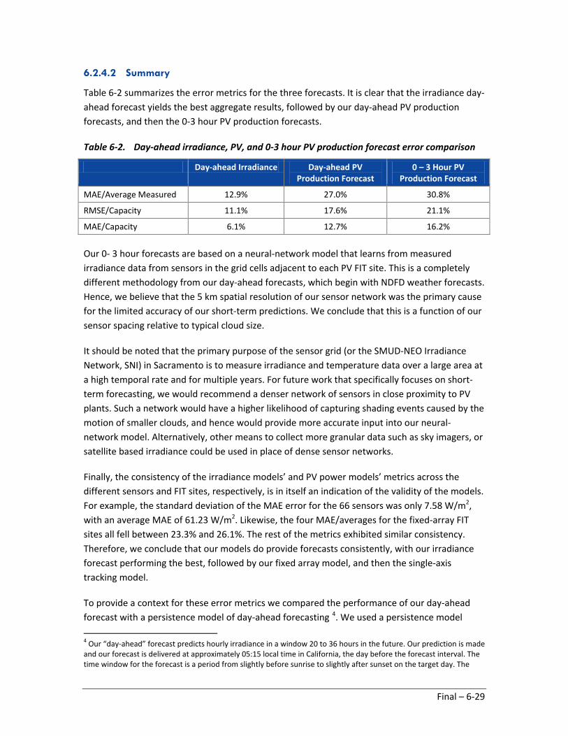
6.2.4.2 Summary

Table 6-2 summarizes the error metrics for the three forecasts. It is clear that the irradiance day-ahead forecast yields the best aggregate results, followed by our day-ahead PV production forecasts, and then the 0-3 hour PV production forecasts.

Table 6-2. Day-ahead irradiance, PV, and 0-3 hour PV production forecast error comparison

Day-ahead Irradiance Day-ahead PV Production Forecast

0 – 3 Hour PV Production Forecast

MAE/Average Measured 12.9% 27.0% 30.8%

RMSE/Capacity 11.1% 17.6% 21.1%

MAE/Capacity 6.1% 12.7% 16.2%

Our 0- 3 hour forecasts are based on a neural-network model that learns from measured irradiance data from sensors in the grid cells adjacent to each PV FIT site. This is a completely different methodology from our day-ahead forecasts, which begin with NDFD weather forecasts. Hence, we believe that the 5 km spatial resolution of our sensor network was the primary cause for the limited accuracy of our short-term predictions. We conclude that this is a function of our sensor spacing relative to typical cloud size.

It should be noted that the primary purpose of the sensor grid (or the SMUD-NEO Irradiance Network, SNI) in Sacramento is to measure irradiance and temperature data over a large area at a high temporal rate and for multiple years. For future work that specifically focuses on short-term forecasting, we would recommend a denser network of sensors in close proximity to PV plants. Such a network would have a higher likelihood of capturing shading events caused by the motion of smaller clouds, and hence would provide more accurate input into our neural-network model. Alternatively, other means to collect more granular data such as sky imagers, or satellite based irradiance could be used in place of dense sensor networks.

Finally, the consistency of the irradiance models’ and PV power models’ metrics across the different sensors and FIT sites, respectively, is in itself an indication of the validity of the models. For example, the standard deviation of the MAE error for the 66 sensors was only 7.58 W/m2, with an average MAE of 61.23 W/m2. Likewise, the four MAE/averages for the fixed-array FIT sites all fell between 23.3% and 26.1%. The rest of the metrics exhibited similar consistency. Therefore, we conclude that our models do provide forecasts consistently, with our irradiance forecast performing the best, followed by our fixed array model, and then the single-axis tracking model.

To provide a context for these error metrics we compared the performance of our day-ahead forecast with a persistence model of day-ahead forecasting 4. We used a persistence model

4 Our “day-ahead” forecast predicts hourly irradiance in a window 20 to 36 hours in the future. Our prediction is made and our forecast is delivered at approximately 05:15 local time in California, the day before the forecast interval. The time window for the forecast is a period from slightly before sunrise to slightly after sunset on the target day. The

Final – 6-29

because it was a means by which we could get a second forecast for the same sites, with the same forecast horizon and with the same averaging interval. The persistence model we used was based upon the measured data from the sensor network and was expressed in kWh/m2/day. To do this we used sensors which we knew had complete uninterrupted data for the same 6-month period as we had used for the previous analysis5. For this persistence model total measured daily kWh/m2 were used as a predictor for total daily kWh/m2 on the subsequent day. For each sensor we summed the daytime hour values in each 24-hour period over the course of the selected 6-month sample period. We then divided the sum of 1-minute measured values by 60. The resulting value is the number of Wh/m2 for the day in question. We divided this value by 1000 to get kWhr/m2 or “sun hours.” The integral of all of the sun hours in a 24-hour period is referred to as equivalent sun hours per day or “ESH/day.” Using this method we calculated a day-ahead forecast of ESH for the latitude and longitude for each sensor based on the previous day’s ESH for that sensor. From this persistence calculation the error metrics (RMSE, MAE, RMSE/average, MAE/average, RMSE/capacity, MAE/capacity) were calculated by comparing the persistence model prediction of ESH to the measured ESH at each sensor site. For a value for capacity, we took the maximum global horizontal ESH for Sacramento of 7.9 kWhr/m2, as reported in the NREL Red Book.

In a similar manner we calculated the ESH for each day of NEO’s day-ahead forecast which was created using NDFD data. From NEO's day-head model the same error metrics were calculated by comparing the NEO model prediction of ESH to the measured ESH at each sensor site. This was necessary to achieve the same forecast horizon and time interval as the persistence model.

Table 6-3 is a comparison of forecast error for all 66 measurement sites for a 6-month period for NEO's NDFD method and the persistence method described above. The NEO RMSE absolute error values are lower by about 0.2 kWhr/m2/day and RMSE relative error values are lower by between 3.5 and 2.6% for NEO's day ahead forecast method than persistence in all cases. However, the MAE, both absolute and relative, are almost identical for NEO and the persistence model. This equivalence in apparent errors may be due to the fact that the Sacramento area has a very high percentage of very clear days, resulting in more instances where the daily ESH from one day are a good predictor of the subsequent day. In addition, the process of aggregating the hourly irradiance data in NEO's day-ahead forecasts into a single daily summation of ESH "throws away" much of the value of the hourly forecast for the NEO model and creates a lower resolution output. This can be seen where the RMSE metrics captures more of the impact of outliers in the dataset than the MAE metric.

choice of when the forecast is delivered, and thus how far in advance the forecast is calculated, is based upon SMUD’s energy trading department schedule. SMUD’s energy trading department plans their purchases and sales in their day-ahead market between 5:00 and 8:00 am each morning for the next day. 5 This is a six month period for which we had sensor data which had been filtered and interpolated using the process developed by Sandia and SMUD.

Final – 6-30

Table 6-3. NEO NDFD day-ahead forecasts compared to a persistence model

Day-Ahead Forecast Models: NEO NDFD vs. Persistence

66 Sensors, Six Months

NEO NDFD Persistence

RMSE (ESH) 0.7249 0.9268

MAE (ESH) 0.4758 0.4761

RMSE/avg (%) 12.41 15.87

MAE/avg (%) 8.14 8.15

RMSE/capacity (7.9) (%) 9.18 11.73

MAE/capacity (7.9) (%) 6.02 6.03

6.3 Production Forecasting Outcomes

6.3.1 5 km Grid Irradiance Network (NEO and SMUD)

This network was up and running by May 31, 2011. It consists of 66 secondary stations (designed and built by NEO) plus six primary stations (RSR2s, designed by Irradiance, Inc.; five of the six were assembled by NEO, one was already in place). This network has provided 24 months of GHI and temperature data, and continues to function.

6.3.2 Forecast PV Production Piece-wise Program (NEO and Contractors)

NEO downloaded required NDFD data manually from NOAA site. NDFD program tkdegrib was run manually to unpack NDFD gridded binary forecast meteorological files. FIT system modules were modeled based upon similarities with modules already in the Sandia module database and the database was updated. NEO created an Excel version of the Sandia PV Array Model for manual processing and sample runs were done.

The final automated forecasting program, DAE_analyze.pl, was coded, and since April 17, 2012, NEO has been sending daily power production forecasts to SMUD.

6.3.3 One Year Measured 5 km, 1 Min Rate, Irradiance and Ambient Temp Data (NEO and Contractors)

As of May 31, 2013, data from the full primary and secondary sensor network is available on the SMUD website. Due to a 1 year extension, as of May 31 the data set contains a full 24 months of data. The full data record can be found on SMUD’s ftp site: ftp://ftp01.smud.org/pub/SNIData/

Final – 6-31

The file will be a zip file, and it will be a backup of NEO's MySQL database table. There is a “read me” file that includes information about the data. The data will include raw shadow events and interpolated values. The data will be updated monthly starting in May 2013.

Review of the data has determined that 98.5% of the data set contains valid and accurate data.

6.3.4 One Year Day-ahead Forecast PV Production Data by Site, 1 Hour Intervals (NEO and Contractors)

NEO created forecasts from May 1, 2012, through April 30, 2013 for the following seven FIT sites:

• Bruceville (18 MW)

• Kammerer (15 MW)

• Eschinger (15 MW)

• Dillard (9.4 MW)

• Kost (3 MW)

• Boessow (3 MW)

• Point Pleasant (1 MW)

NEO created forecasts from only November 16, 2012, to April 30, 2013, for the eighth FIT site, McKenzie (30 MW), since this site did not come on-line until November 2012. These forecasts can be found on SMUD’s ftp site and the CSI RD&D website6, in the spreadsheet entitled: http://www.calsolarresearch.org/images/stories/documents/Sol1_funded_proj_docs/SMUD/Deliverable-IV_PV-Production_Day-Ahead-Forecasts_130610.xlsx.

The spreadsheet also contains the measured power for each FIT site to allow for easy comparison.

6.3.5 One Year 3­hour Forecast PV Production Data by Site, 15 Min Intervals (NEO and Contractors)

NEO created forecasts from February 1, 2012, through November 30, 2012, for the following seven FIT sites:

• Bruceville (18 MW)

• Kammerer (15 MW)

• Eschinger (15 MW)

• Dillard (9.4 MW)

6 http://calsolarresearch.ca.gov/funded-projects/66-high-penetration-pv-initiative

Final – 6-32

• Kost (3 MW)

• Boessow (3 MW)

• Point Pleasant (1 MW)

NEO created forecasts from only November 16, 2012, to November 30, 2012, for the eighth FIT site, McKenzie (30 MW) since this site did not come on-line until November 2012. These forecasts can be found on SMUD’s ftp site and the CSI RD&D website, in the spreadsheet entitled: Deliverable V_PV Production 0-3 Hour Forecasts 130610.xlsx.

The spreadsheet also contains the measured power for each FIT site to allow for easy comparison. There are also 10 spreadsheets that contain 0-3 hour forecast and measured GHI for 72 5 km grid cells that make up the SNI network. Each spreadsheet contains 1 month worth of data for every grid cell.

6.4 Production Forecasting Lessons Learned

1. Mounting secondary stations on existing utility poles had the unexpected consequence of requiring post collection data filtering. Shadows from overhead wires and crosstrees caused drops in GHI levels as the sun moved across the sky. These were very noticeable on clear days. For future installations on utility poles, we recommend further developing and automating the filtering algorithm developed by SMUD and Sandia. Where possible, we recommend placing the devices only on poles without crosstrees.

2. Future installations of a network of irradiance sensors such as the one installed under this grant should include a means for calibrating the sensors to ensure accurate measurements. NEO and SMUD installed four PSPs in our network as reference devices for use in calibrating all the other pyranometers. However, these devices were an afterthought rather than a planned component. Similarly, our global calibration methodology for this project was developed after the sensors were installed. Future projects of this nature should have a calibration plan included as part of the initial scope of work.

3. The NDFD data we used in our 20- 36 hour forecast model had 3-hour forecast periods (time intervals) for most parameters, e.g., 0600- 0900, 0900-1200, etc.). Since we were forecasting irradiance and power production every hour, these intervals were not optimal. In addition, the forecast period for a key parameter—sky cover—varied between geographic locations, further complicating our modeling efforts. The lesson here is that there (now) exists a better resource—the high resolution rapid refresh (HRRR) forecast. This forecast has shorter forecast periods (1 hour) and smaller geographic size (3 km vs. 5 km grid) and a larger number of critical parameters.

4. Some of the RSRs used in the network were connected via short-haul modem to SMUD’s SCADA network. Occasionally their internal clocks would be reset to local time vs. Greenwich mean time. This caused a misalignment of time/date stamps for the daily

Final – 6-33

collected data. For future work, any programming and data logger clock resets need to be limited to the network’s administrator only (in this case, NEO).

5. To improve PV plant modeling, better access to plant data, especially back-tracking algorithms, should be made available to the forecasters. In addition, to improve the accuracy of forecast metrics, plant availability (i.e., down times for maintenance) should be provided to the forecasters. In this current project, NEO was not told of these down times, and hence had to make some assumptions while comparing forecast to actual plant production (if the measured output of a plant was zero 2 days straight, for example, we assumed it was off line, and did not use those days in our metrics).

6. Lessons learned in this research which are immediately applicable include the use of a utility's full asset base as potential platforms for irradiance measurement and conduits for irradiance data. Asset base includes utility poles, substations, maintenance and office buildings, communications networks, and AMI. NEO's demonstrated capability for providing day-ahead forecasts for SMUD's 100 MWs of feed-in-tariff (FIT) sites using open source meteorological data from the National Digital Forecast Database (NDFD) or other sources is a process that can be duplicated by any of California's utilities.

Final – 6-34

7.0 LESSONS LEARNED

The PV integration studies summarized in this document include diverse aspects of PV power generation and distribution. These PV studies are all based on connection of the PV generation into existing distribution systems at sub-transmission voltages. The PV generation must be evaluated in the context of the distribution systems that the PV is connected to due to the potentially high percentage of power injected by the PV generation.

PV evaluations will, therefore, require a much more granular analysis of existing loads, energy time of use, and will require substantially more monitoring than previous generation sources. Essentially, PV will be a major driver for a smart grid—the timing of these two technologies will enable increased system reliability, efficiency, with (ultimately) greater customer satisfaction.

Rather than reiterate the specific findings presented herein by each study, a few general lessons learned are provided:

• Analysis of a single feeder with moderate or high solar penetration points is difficult due to the interaction of that feeder on the substation bus. PV analysis and modeling should include consideration of impacts at the substation bus level.

• The granularity of distribution system data is specific to the type of analysis desired, and to the type of equipment being evaluated. Certain load data may be collected at longer time intervals, but transformer tap changer evaluation must be conducted with short time interval data.

• Feeders must also be individually considered by the planner, based on installed equipment, line characteristics, loads, and monitoring data.

• Communication and monitoring systems are still in the initial stages of implementation. Further standardization of communications between PV sources and the utility will improve the quality of data and improve system security.

• Utility customers will play a critical part in PV acceptance and integration at the distribution level. By providing user-friendly monitoring data, utility customers become more involved with their electrical use, are excited by PV generation features, and may be encouraged by their conservation measures.

• PV production forecasting is still in a developmental stage. The difficulties in irradiance data collection and quality impacted predictions, as did some of the modeling software.

• PV forecasting is considered to be much better at shorter time intervals, smaller geographic sizes, and by including more system data parameters.

Final – 7-1

8.0 GENERAL CONCLUSIONS

The production of this High Penetration PV Initiative study summary represents major efforts by SMUD and the Hawaiian electrical utilities to understand the impacts of solar power generation on their distribution systems. The utilities are responding to an entirely new paradigm of distributed renewable power generation, which is often sporadic and difficult to predict. The utilities are using the latest smart grid technologies to monitor, simulate, and forecast impacts on the distribution systems. What we see in these studies is the incremental development of smart grid devices, methodologies and tools, which all warrent further study and research.

The tools necessary for complete understanding of distribution system impacts are not completely evolved at this stage, but the tools and techniques are becoming more useful and available. Monitoring points are not standard and often they are inadequate to provide the data necessary for optimal system operation and planning. The simulation software is useful and has some degree of accuracy, but significant improvements are still needed. Forecasting of PV generation is still very dependent on accurate incoming data, but the data available may be insufficient and incomplete, and data collection systems need greater reliability. The variability of the weather, especially cloud cover in certain regions of Hawaii, appears to be a significant challenge even over small geographic areas.

The general conclusion is that utilities are making greater use of smart grid monitoring devices to assist with PV generation planning, operation, and forecasting. The systems to date are often still in the experimental stages in several aspects, but are improving with each application and effort to further understand the impacts of high penetration solar PV.

This study also points to a more global need for improvements to power distribution system equipment. In particular, equipment to help control load and voltage will go a long way toward improving distribution operations. Energy storage, more rapid response of voltage control devices, and integration of solar inverter control systems into distribution system control will allow greater PV penetration and will provide utilities with improved operational control.

Final – 8-1