S-Step and Communication-Avoiding Iterative Methods

Maxim NaumovNVIDIA, 2701 San Tomas Expressway, Santa Clara, CA 95050

Abstract

In this paper we make an overview of s-step Conjugate Gradient and develop anovel formulation for s-step BiConjugate Gradient Stabilized iterative method. Also,we show how to add preconditioning to both of these s-step schemes. We explain theirrelationship to the standard, block and communication-avoiding counterparts. Finally,we explore their advantages, such as the availability of matrix-power kernel Akx and useof block-dot products B = XTY that group individual dot products together, as wellas their drawbacks, such as the extra computational overhead and numerical stabilityrelated to the use of monomial basis for Krylov subspace Ks = {r, Ar, ..., As−1r}. Wenote that the mathematical techniques used in this paper can be applied to othermethods in sparse linear algebra and related fields, such as optimization.

1 Introduction

In this paper we are concerned with investigating iterative methods for the solution oflinear system

Ax = f (1)

where nonsingular coefficient matrix A ∈ Rn×n, right-hand-side (RHS) f and solutionx ∈ Rn. A comprehensive overview of standard iterative methods can be found in [1, 17].In this brief study we will focus on two popular algorithms: (i) Conjugate Gradient (CG)and (ii) BiConjugate Gradient Stabilized (BiCGStab) Krylov subspace iterative methods.These algorithms are often used to solve linear systems with symmetric positive definite(SPD) and nonsymmetric coefficient matrices, respectively.

NVIDIA Technical Report NVR-2016-003, April 2016.c© 2016 NVIDIA Corporation. All rights reserved.

This research was developed, in part, with funding from the Defense Advanced Research Projects Agency(DARPA). The views, opinions, and findings contained in this article are those of the author and shouldnot be interpreted as representing the official views or policies of the Department of Defense or the U.S.Government.

1

The CG and BiCGStab methods have already been generalized to their block counter-parts in [11, 15]. The block methods work with s vectors simultaneously and were originallydesigned to solve linear systems with multiple RHS, such as

AX = F (2)

where multiple RHS and solutions are column vectors in tall matrices F and X ∈ Rn×s,respectively. However, they can be adapted to solve systems with a single RHS, by forexample randomly selecting the remaining s − 1 RHS [14]. In the latter case, the blockmethods often perform less iterations than their standard counterparts, but they do notcompute exactly the same solution in i iterations as the standard methods in i×s iterations.

The s-step methods occupy a middle ground between their standard and block coun-terparts. They are usually applied to linear systems with a single RHS, they work with svectors simultaneously, but they are also designed to produce identical solution in i iter-ations as the standard methods in i× s iterations, when the computation is performed inexact arithmetic. In fact, the s-step methods can be viewed as an unrolling of s iterationsand a clever re-grouping of recurrence terms in them.

The s-step methods were first investigated by J. Van Rosendale, A. T. Chronopoulosand C. W. Gear in [4, 6, 16], where the authors proposed s-step CG algorithm for SPDlinear systems. Subsequent work by A. T. Chronopoulos and C. D. Swanson in [5, 7] leadto the development of s-step methods, such as GMRES and Orthomin, but not BiCGStab,for nonsymmetric linear systems. These methods were further improved and generalizedto the solution of eigenvalue problems using Lanczos and Arnoldi iterations in [8, 9].

There are several advantages for using s-step methods. The first advantage is that thematrix-vector multiplications used to build the Krylov subspace Ks = {r, Ar, ..., As−1r}can be performed together, one immediately after another. This allows us to develop amore efficient matrix-vector multiplication, using a pipeline where the results from currentmultiplication are immediately forwarded as inputs to the next. The second advantage isthat the dot products spread across multiple iterations are bundled together. This allowsus to minimize fan-in communication that is associated with dot-products and often limitsscalability of parallel platforms.

There are also some disadvantages for using s-step methods. We perform more workper 1 iteration of an s-step method than per s iterations of a standard method. The extrawork is often the result of one extra matrix-vector multiplication required to recomputethe residual. Also, notice that in practice the vectors computed by matrix-power kernelAkx for k = 0, ..., s− 1 quickly become linearly dependent. Therefore, s-step methods cansuffer from issues related to numerical stability resulting from the use of a monomial basisfor the Krylov subspace corresponding to s internal iterations.

In this paper we first make an overview of how to use properties of the directions andresidual vectors in standard CG to build the s-step CG iterative method. Then, we findthe properties of the directions and residual vectors in standard BiCGStab. Finally, we usethis information in conjuction with recurrence relationships for these vectors to developa novel s-step BiCGStab iterative method. We also show how to add preconditioning toboth of these s-step schemes.

2

Finally, we point out that s-step iterative methods are closely related to communication-avoiding algorithms proposed in [2, 3, 10, 12]. In fact, the main differences between thesemethods lie in (i) a different basis used by the communication-avoiding algorithms toaddress numerical stability, and (ii) an efficient (communication-avoiding) implementationof matrix-power kernel Akx as well as distributed dense linear algebra operations, such asdense QR-factorization used in GMRES [18].

Let us now show how to derive the well known s-step CG and novel s-step BiCGStabiterative methods as well as how to add preconditioning to both algorithms.

2 S-Step Conjugate Gradient (CG)

The standard CG method is shown in Alg. 1.

Algorithm 1 Standard CG

1: Let A ∈ Rn×n be a SPD matrix and x0 be an initial guess.2: Compute r0 = f−Ax0

3: for i = 0, 1, ...until convergence do4: if i == 0 then . Find directions p5: Set pi = ri6: else7: Compute βi =

rTi rirTi−1ri−1

. Dot-product

8: Compute pi = ri + βipi−1

9: end if10: Compute qi = Api . Matrix-vector multiply

11: Compute αi =rTi rirTi qi

. Dot-product

12: Compute xi+1 = xi + αipi13: Compute ri+1 = ri − αiqi14: if ||ri+1||2/||r0||2 ≤ tol then stop end . Check Convergence15: end for

Let us now prove that the directions pi and residuals ri computed by CG satisfy a fewproperties. These properties will subsequently be used to setup the s-step CG method.

Lemma 1. The residuals ri are orthogonal and directions pi are A-orthogonal

rTi rj = 0 and pTi Apj = 0 for i 6= j (3)

Proof. See Proposition 6.13 in [17].

Theorem 1. The current residual ri and all previous direction pj are orthogonal

rTi pj = 0 for i > j (4)

3

Proof. Using induction. Notice that for the base case i = 1 we have

rT1 p0 = rT1 r0 = 0 (5)

For the induction step, let us assume rTi pj−1 = 0. Then

rTi pj = rTi (rj + βj−1pj−1) = βj−1rTi pj−1 = 0 (6)

Let us now derive an alternative expression for scalars αi and βi.

Corollary 1. The scalars αi and βi satisfy

(pTi Api)αi = pTi ri (7)

(pTi Api)βi = −pTi Ari+1 (8)

Proof. Using Lemma 1 and Theorem 1 we have

rTi ri+1 = rTi (ri − αiApi) = (pi − βi−1pi−1)T ri − αi(pi − βi−1pi−1)TApi

= pTi ri − αipTi Api = 0 (9)

and

pTi Api+1 = pTi A(ri+1 + βiApi) = pTi Ari+1 + βipTi Api = 0 (10)

Let us now assume that we have s directions pi available at once, then we can write

xi+s = xi + αipi + ...+ αi+s−1pi+s−1 = xi + Piai (11)

where Pi = [pi, ...,pi+s−1] ∈ Rn×s is a tall matrix and ai = [αi, ..., αi+s−1]T ∈ Rs is a smallvector. Consequently, residual can be expressed as

ri+s = f−Axi+s = ri −APiai (12)

Also, let us assume that we have the monomial basis for Krylov subspace for s iterations

Ri = [ri, Ari, ..., As−1ri] (13)

Then, following the standard CG algorithm, it would be natural to express the next direc-tions as a combination of previous directions and the basis vectors

Pi+1 = Ri+1 + PiBi (14)

where Bi = [βi,j ] ∈ Rs×s is a small matrix. At this point we have almost all the buildingblocks of s-step CG method, but we are still missing a way to find scalars α and β stored inthe vector ai and matrix Bi. These coefficients can be found using the following Corollary.

4

Corollary 2. The vector aTi = [αi, ..., αi+s−1] and matrix Bi = [βi,j ] satisfy

(P Ti APi)ai = P Ti ri (15)

(P Ti APi)Bi = −P Ti ARi+1 (16)

Proof. Enforcing orthogonality of residual and search directions in Theorem 1 we have

P Ti ri+s = P Ti (ri −APiai) = P Ti ri − (P Ti APi)ai = 0 (17)

Also, enforcing A-orthogonality between search directions in Lemma 1 we obtain

P Ti APi+1 = P Ti A(Ri+1 + PiBi) = P Ti ARi+1 + (P Ti APi)Bi = 0 (18)

Notice the similarity between Corollary 1 and 2 for standard and s-step CG, respectively.Finally, putting all the equations (11) - (16) together we obtain the pseudo-code for

s-step CG iterative method, shown in Alg. 2.

Algorithm 2 S-Step CG

1: Let A ∈ Rn×n be a SPD matrix and x0 be an initial guess.2: Compute r0 = f−Ax0 and let index k = is (initially k = 0)3: for i = 0, 1, ...until convergence do4: Compute T = [rk, Ark, ..., A

srk] . Matrix-power kernel5: Let Ri = [rk, Ark, ..., A

s−1rk] . Extract R = T (:, 1 : s− 1) from T6: Let Qi = [Ark, A

2rk, ..., Asrk] = ARi . Extract Q = T (:, 2 : s) from T

7: if i == 0 then . Find directions p8: Set Pi = Ri9: else

10: Compute Ci = −QTi Pi−1 . Block dot-products11: Solve Wi−1Bi = Ci . Find scalars β12: Compute Pi = Ri + PiBi13: end if14: Compute Wi = QTi Pi . Block dot-products15: Compute gi = P Ti ri16: Solve Wiai = gi . Find scalars α17: Compute xk+s = xk + Piai . Compute new approximation xk18: Compute rk+s = f−Axk+s . Recompute residual rk19: if ||rk+s||2/||r0||2 ≤ tol then stop end . Check Convergence20: end for

5

Let us now introduce preconditioning into the s-step CG in a manner similar to thestandard algorithm. Let the preconditioned linear system be

(L−1AL−T )(LTx) = L−1f (19)

Then, we can apply the s-step on the preconditioned system (19) and re-factor recur-rences in terms of preconditioner M = LLT . If we express everything in terms of “precon-ditioned” directions M−1Pi and work with the original solution vector xi we obtain thepreconditioned s-step CG method, shown in Alg. 3.

Notice that tall matrices Zi and Qi on lines 6 and 7 can be constructed during thecomputation of T on line 5 in Alg. 3. The key observation is that the computation of Tproceeds in the following fashion

ri,M−1ri, (AM

−1)ri,M−1(AM−1)ri, (AM

−1)2ri, ...,M−1(AM−1)s−1ri, (AM

−1)sri

and therefore alternating odd and even terms define columns of tall matrices Zi and Qi.

Algorithm 3 Preconditioned S-Step CG

1: Let A ∈ Rn×n be a SPD matrix and x0 be an initial guess.2: Let M = LLT be SPD preconditioner, so that M−1 ≈ A−1.3: Compute r0 = f−Ax0, r0 = M−1r0 and let index k = is (initially k = 0)4: for i = 0, 1, ...until convergence do5: Compute T = M−1[rk, Ark, ..., A

srk] . Matrix-power kernel6: Let Zi = M−1[rk, Ark, ..., A

s−1rk] = M−1Ri . Build Z & Q during7: Let Qi = [Ark, A

2rk, ..., Asrk] = AZi . computation of T

8: where auxiliary A = AM−1 and Ri = [rk, Ark, ..., As−1rk]

9: if i == 0 then . Find directions p10: Set Pi = Zi11: else12: Compute Ci = −QTi Pi−1 . Block dot-products13: Solve Wi−1Bi = Ci . Find scalars β14: Compute Pi = Zi + PiBi15: end if16: Compute Wi = QTi Pi . Block dot-products17: Compute gi = P Ti ri18: Solve Wiai = gi . Find scalars α19: Compute xk+s = xk + Piai . Compute new approximation xk20: Compute rk+s = f−Axk+s . Recompute residual rk21: Compute rk+s = M−1rk+s

22: if ||rk+s||2/||r0||2 ≤ tol then stop end . Check Convergence23: end for

6

Finally, notice that preconditioned s-step CG performs an extra matrix-vector multi-plication with A and preconditioner solve with M−1 per 1 iteration, when compared withs iterations of the standard preconditioned CG method. The extra work happens duringre-computation of residual at the end of every s-step iteration.

3 S-Step BiConjugate Gradient Stabilized (BiCGStab)

Let us now focus on the s-step BiCGStab method, which has not been previously derivedby A. T. Chronopoulos et al. The standard BiCGStab is given in Alg 4.

Algorithm 4 Standard BiCGStab

1: Let A ∈ Rn×n be a nonsingular matrix and x0 be an initial guess.2: Compute r0 = f−Ax0 and set p0 = r0

3: Let r0 be arbitrary (for example r0 = r0)4: for i = 0, 1, ...until convergence do5: Compute zi = Api . Matrix-vector multiply

6: Compute αi =rT0 rirT0 zi

. Dot-product

7: Compute si = ri − αizi . Find directions s8: if ||si||2/||r0||2 ≤ tol then set xi+1 = xi + αipi and stop end . Early exit9: Compute vi = Asi . Matrix-vector multiply

10: Compute ωi =sTi vi

vTi vi

. Dot-product

11: Compute xi+1 = xi + αipi + ωisi12: Compute ri+1 = si − ωivi13: if ||ri+1||2/||r0||2 ≤ tol or early exit then stop end . Check Convergence

14: Compute βi =(rT0 ri+1

rT0 ri

)(αiωi

)15: Compute pi+1 = ri+1 + βi(pi − ωizi) . Find directions p16: end for

Recall that the directions pi and residuals ri in BiCGStab have been derived fromBiCG method using polynomial recurrences to avoid multiplication with transpose of thecoefficient matrix AT [17]. The properties of directions and residuals in BiCG methodare well known and can be easily used to setup the corresponding s-step method. Therelationships between them in BiCGStab are far less clear. Therefore, the first step is tounderstand the properties of directions si, pi and residuals ri, r0 in BiCGStab method.

Theorem 2. The directions si, pi and residuals ri, r0 satisfy the following relationships

rT0 si = 0 (20)

rTi+1Asi = 0 (21)

rT0 (pi+1 − βipi) = 0 (22)

7

Proof. First relationship (20) follows from

rT0 si = rT0 (ri − αiApi) = rT0 ri − αirT0 Api = rT0 ri − rT0 ri = 0 (23)

Second relationship (21) follows from

rTi+1Asi = (si − ωiAsi)TAsi = sTi Asi − ωi(Asi)T (Asi) = sTi Asi − sTi Asi = 0 (24)

The last relationship (22) follows from

rT0 (pi+1 − βipi) = rT0 (ri+1 − βiωiApi) = (25)

= rT0 ri+1 −(rT0 ri+1

rT0 Api

)rT0 Api = 0 (26)

Notice that we can express the recurrences of BiCGStab in the following convenient form

si = ri − αiApi (27)

ri+1 = (I − ωiA)si (28)

qi = (I − ωiA)pi (29)

pi+1 = ri+1 + βiqi (30)

Corollary 3. Let auxiliary vector yi = si + βipi, then directions pi+1 = (I − ωiA)yi and

rT0 Ayi = 0 (31)

as long as ωi 6= 0.

Proof. Notice that using recurrences (28), (29) and (30) we have

pi+1 = ri+1 + βiqi = (I − ωiA)si + βi(I − ωiA)pi = (I − ωiA)(si + βipi) (32)

and using first and last relationships in Theorem 2 we have

rT0 A(si + βipi) = − 1

ωirT0 A(−ωisi − βiωipi) = − 1

ωirT0 (si − ωiAsi − βiωiApi)

= − 1

ωirT0 (ri+1 − βiωiApi) = − 1

ωirT0 (pi+1 − βipi) = 0 (33)

These properties are interesting by themselves, but it is difficult to rely only on themto setup a linear system for finding scalars α, ω and β similarly to CG and BiCG methodsbecause they involve a single vector corresponding to the shadow residual r0, rather than alldirections p in CG or shadow directions p in BiCG. Therefore, we have to find additionalconditions and a different way of setting up the s-step method.

8

Let us now assume that we have s directions pi and si available at once, then we have

xi+s = xi + αipi + ...+ αi+s−1pi+s−1 + ωisi + ...+ ωi+s−1si+s−1

= xi + Piai + Sioi (34)

where Pi = [pi, ...,pi+s−1] and Si = [si, ..., si+s−1] ∈ Rn×s are tall matrices and ai =[αi, ..., αi+s−1]T and oi = [ωi, ..., ωi+s−1]T ∈ Rs are small vectors. Consequently, residualcan be expressed as

ri+s = f−Axi+s = ri −A(Piai + Sioi) (35)

Also, let us assume that we have the monomial basis for Krylov subspace for s iterations

Ri = [ri, Ari, ..., A2(s−1)ri] (36)

and monomial basis for directions

Pi = [pi, Api, ..., A2(s−1)pi] (37)

Notice that using recurrences (27) - (30) we can write the following

[si, Asi,qi, Aqi] =[ri, Ari, A

2ri,pi, Api, A2pi]C (38)[

ri+1,pi+1

]= [si, Asi,qi, Aqi]D (39)

where transitional matrices of scalar coefficients C and D are

C = C(1)C(2) =

11

01 0

−αi 1 0−αi 1

1

11

−ωi 1−ωi

=

11

01 0

−αi −ωi 1−αi −ωi

(40)

and

D = D(1)D(2) =

1

−ωi 01 0

1

1 1

βi0

=

1 1

−ωi −ωiβi0

(41)

9

Also, note that for B = CD and k ≥ 0 we have

Ak[ri+1,pi+1] = Ak[ri, Ari, A2ri,pi, Api, A

2pi]B (42)

Therefore, letting Bi ∈ R4s−2×4s−6 follow the same pattern as B we have

[ri+1, ..., A2(s−2)ri+1,pi+1, ..., A

2(s−2)pi+1] = [ri, ..., A2(s−1)ri,pi, ..., A

2(s−1)pi]Bi (43)

and consequently

[ri+s−1,pi+s−1] = [ri, ..., A2(s−1)ri,pi, ..., A

2(s−1)pi]Bi...Bi+s−2 (44)

Hence, we can use (44) to build directions si, pi and residuals ri after s− 1 iterations, aslong as we are able to compute the scalars α, ω and β used in transitional matrices.

Let us now compute the matrix W ∈ R4s−2×4s−2 and vector w ∈ R4s−2 such that

Wi = [Ri, Pi]T [Ri, Pi] (45)

wTi = rT0 [Ri, Pi] = [gTi ,h

Ti ] (46)

and let Wi(j, k) denote j-th row and k-th column element of matrix Wi, while wi(j) denotesthe j-th element of vector wi. Also, let us use 1-based indexing.

Then,

αi =rT0 ri

rT0 Api=

gi(1)

hi(2)(47)

Further, after updating

W′i = C

(1)i

TWiC

(1)i (48)

we have

ωi =sTi Asi

(Asi)T (Asi)=W′i (1, 2)

W′i (2, 2)

(49)

and, after updating

w′i = (CiD

(1)i )Twi (50)

we obtain

βi =

(rT0 ri+1

rT0 ri

)(αiωi

)=

(w′i(1)

gi(1)

)(αiωi

)(51)

Finally,

Wi+1 = (C(2)i Di)

TW′i (C

(2)i Di) = BT

i WiBi (52)

and

wi+1 = D(2)i

Tw′i = BT

i wi (53)

Finally, putting all the equations (34) - (53) together we obtain the pseudo-code fors-step BiCGStab iterative method, shown in Alg. 5.

10

Algorithm 5 S-Step BiCGStab

1: Let A ∈ Rn×n be a nonsingular coefficient matrix and let x0 be an initial guess.2: Compute r0 = f−Ax0 and set p0 = r0

3: Let r0 be arbitrary (for example r0 = r0) and let index k = is+ j (initially k = 0)4: for i = 0, 1, ...until convergence do5: Compute T = [[rk,pk], A[rk,pk], ..., A

2s[rk,pk]] . Matrix-power kernel6: Let Ri = [rk, Ark, ..., A

2srk] = [Ri, A2srk] . Extract R from T

7: Let Pi = [pk, Apk, ..., A2spk] = [Pi, A

2spk] = [pk, Pi] . Extract P from T8: Compute Wi = [Ri, Pi]

T [Ri, Pi] . Block dot-products9: Compute wT

i = rT0 [Ri, Pi] = [gTi ,hTi ]

10: Let . and . indicate all but last and first elements of ., as shown for Ri and Pi11: for j = 0, ..., s− 1 do

12: Set αk = gk(1)hk(2) and store ai(j) = αk . Note αk =

rT0 rkrT0 Apk

13: Compute Sk = Rk − αkPk . Sk = [sk, Ask, ..., A2(s−j)−1sk]

14: Update W′k = C

(1)k

TWkC

(1)k . Using sk = rk − αkApk

15: if√W′k(1, 1)/||r0||2 ≤ tol then break end . Check ||sk||22 for early exit

16: Set ωk =W′k(1,2)

W′k(2,2)

and store oi(j) = ωk . Note ωk =sTkAsk

(Ask)T (Ask)

17: Compute Qk = Pk − ωkPk . Qk = [qk, Aqk, ..., A2(s−j)−1qk]

18: if (j == s− 1) then break; . Check for last iteration19: Compute Rk+1 = Sk − ωkSk . Rk+1 = [rk+1, .., A

2(s−j)−2rk+1]

20: Update w′k = (CkD

(1)k )Twk . Using rk+1 = sk − ωkAsk

21: Set βk =

(w′k(1)

gk(1)

)(αkωk

). Note βk =

(rT0 rk+1

rT0 rk

)(αkωk

)22: Compute Pk+1 = Rk+1 + βkQk . Pk+1 = [pk+1, .., A

2(s−j)−2pk+1]23: Update Wk+1 = BT

kWkBk . Using pk+1 = rk+1 + βkqk24: Update wk+1 = BT

k wk

25: end for26: Let Pi = [pi, ...,pk−1] and Si = [si, ..., sk−1] have the constructed directions27: Compute xi+s = xi + Piai + Sioi . Do not use last sk−1 if early exit28: Compute ri+s = f−Axi+s . Note k = is+ s− 1 unless early exit29: if ||ri+s||2/||r0||2 ≤ tol or early exit then stop end . Check Convergence

30: Compute βk =(rT0 ri+s

gk(1)

)(ai(s−1)oi(s−1)

). Note αk = ai(s− 1) and ωk = oi(s− 1)

31: Compute pi+s = ri+s + βkqk32: end for

11

It is worthwhile to mention again that updates using transitional matrices of scalarcoefficients Bi = CiDi can be expressed in terms of recurrences. In fact notice that matricesC(1), C(2), D(1), D(2) in equations (40) - (41) have one-to-one correspondence to recurrencesin equations (27) - (30). We use a mix of transitional matrices and recurrences for clarity inthe pseudo-code. However, we point out that latter allows for more efficient implementationof the algorithm in practice.

Also, notice that at each inner iteration the size of tall matrices Ri and Pi as wellas small square matrix Wi and vector wi is reduced by 4 elements (columns for Ri andPi, rows/columns for Wi and vector elements for wi). These 4 elements correspond to twoextra powers of A and A2 applied to residual r and directions p. Consequently, the updatescan be done in-place preserving all previously computed residuals and directions withoutrequiring extra memory storage for them.

Let us now introduce preconditioning into the s-step BiCGStab in a manner similar tothe standard algorithm. Let the preconditioned linear system be

(AM−1)(Mx) = f (54)

Then, we can apply the s-step on the preconditioned system (54) and re-factor recur-rences in terms of preconditioner M = LU . If we express everything in terms of “precon-ditioned” directions M−1Pi and M−1Si and work with the original solution vector xi weobtain the preconditioned s-step BiCGStab method, shown in Alg. 6.

Notice that tall matrices Ri, Pi, Vi and Zi on lines 7 − 10 can be constructed duringthe computation of T on line 6 in Alg. 6. The key observation is that the computation ofT proceeds in the following fashion

[ri,pi], M−1[ri,pi],

(AM−1)[ri,pi], M−1(AM−1)[ri,pi],

...

(AM−1)2s−1[ri,pi],M−1(AM−1)2s−1[ri,pi],

(AM−1)2s[ri,pi] (55)

and therefore terms in first and second column define tall matrices Ri, Pi, Vi and Zi.It is important to point out that in preconditioned s-step BiCGStab we carry both Ri,

Pi and Vi, Zi through inner s− 1 iterations. The latter pair is needed to compute originalxi+s on line 30 and then residual ri+s on line 31, while the former pair is needed to computedirection pk on line 35 in Alg. 6. Both residual rk and direction pk are needed to computeT in the next outer iteration. Notice that this is different from preconditioned s-step CG,where only preconditioned residual rk is needed for the next outer iteration.

Finally, notice that preconditioned s-step BiCGStab performs an extra matrix-vectormultiplication with A and preconditioner solve with M−1 per 1 iteration, when comparedwith s iterations of the standard preconditioned BiCGStab method. The extra work hap-pens during re-computation of residual at the end of every s-step iteration.

12

Algorithm 6 Preconditioned S-Step BiCGStab

1: Let A ∈ Rn×n be a nonsingular coefficient matrix and let x0 be an initial guess.2: Let M = LU be the preconditioner, so that M−1 ≈ A−1.3: Compute r0 = f−Ax0 and set p0 = r0

4: Let r0 be arbitrary (for example r0 = r0) and let index k = is+ j (initially k = 0)5: for i = 0, 1, ...until convergence do6: Compute T = [[rk,pk], A[rk,pk], ..., A

2s[rk,pk]] with A = AM−1 . Matrix-power kernel7: Let Ri = [rk, Ark, ..., A

2srk] = [Ri, A2srk] . Build R, P , V and Z

8: Let Pi = [pk, Apk, ..., A2spk] = [Pi, A

2spk] = [pk, Pi] . during comput. of T9: Let Vi = M−1[rk, Ark, ..., A

2s−1rk] = M−1Ri10: Let Zi = M−1[pk, Apk, ..., A

2s−1pk] = M−1Pi11: Compute Wi = [Ri, Pi]

T [Ri, Pi] . Block dot-products12: Compute wT

i = rT0 [Vi, Zi] = [gTi ,hTi ]

13: Let . and . indicate all but last and first elements of ., as shown for Ri and Pi14: for j = 0, ..., s− 1 do

15: Set αk = gk(1)hk(2) and store ai(j) = αk . Note αk =

rT0 rkrT0 Apk

16: Compute [Sk, S′k] = [Rk, Vk]− αk[Pk, Zk] . Sk = [sk, Ask, ..., A

2(s−j)−1sk]

17: Update W′k = C

(1)k

TWkC

(1)k . Using sk = rk − αkApk

18: if√W′k(1, 1)/||r0||2 ≤ tol then break end . Check ||sk||22 for early exit

19: Set ωk =W′k(1,2)

W′k(2,2)

and store oi(j) = ωk . Note ωk =sTkAsk

(Ask)T (Ask)

20: Compute [Qk, Q′k] = [Pk, Zk]− ωk[Pk, Zk] . Qk = [qk, Aqk, ..., A

2(s−j)−1qk]21: if (j == s− 1) then break; . Check for last iteration22: Compute [Rk+1, Vk+1] = [Sk, S

′k]− ωk[Sk, S′k] . Rk+1 = [rk+1, .., A

2(s−j)−2rk+1]

23: Update w′k = (CkD

(1)k )Twk . Using rk+1 = sk − ωkAsk

24: Set βk =

(w′k(1)

gk(1)

)(αkωk

). Note βk =

(rT0 rk+1

rT0 rk

)(αkωk

)25: Compute [Pk+1, Zk+1] = [Rk+1, Vk+1] + βk[Qk, Q

′k] . Pk+1 = [pk+1, .., A

2(s−j)−2pk+1]26: Update Wk+1 = BT

kWkBk . Using pk+1 = rk+1 + βkqk27: Update wk+1 = BT

k wk

28: end for29: Let Zi = M−1[pi, ...,pk−1] and S′i = M−1[si, ..., sk−1] have the constructed directions30: Compute xi+s = xi + Ziai + S′ioi . Do not use last sk−1 if early exit31: Compute ri+s = f−Axi+s . Note k = is+ s− 1 unless early exit32: if ||ri+s||2/||r0||2 ≤ tol or early exit then stop end . Check Convergence33: Compute r′i+s = M−1ri+s

34: Compute βk =

(rT0 r′i+s

gk(1)

)(ai(s−1)oi(s−1)

). Note αk = ai(s− 1) and ωk = oi(s− 1)

35: Compute pi+s = ri+s + βkqk36: end for

13

4 Numerical Experiments

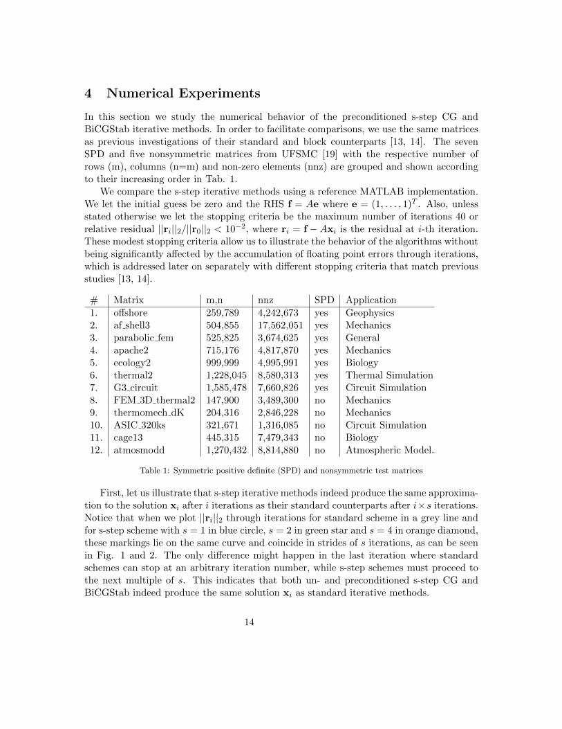
In this section we study the numerical behavior of the preconditioned s-step CG andBiCGStab iterative methods. In order to facilitate comparisons, we use the same matricesas previous investigations of their standard and block counterparts [13, 14]. The sevenSPD and five nonsymmetric matrices from UFSMC [19] with the respective number ofrows (m), columns (n=m) and non-zero elements (nnz) are grouped and shown accordingto their increasing order in Tab. 1.

We compare the s-step iterative methods using a reference MATLAB implementation.We let the initial guess be zero and the RHS f = Ae where e = (1, . . . , 1)T . Also, unlessstated otherwise we let the stopping criteria be the maximum number of iterations 40 orrelative residual ||ri||2/||r0||2 < 10−2, where ri = f − Axi is the residual at i-th iteration.These modest stopping criteria allow us to illustrate the behavior of the algorithms withoutbeing significantly affected by the accumulation of floating point errors through iterations,which is addressed later on separately with different stopping criteria that match previousstudies [13, 14].

# Matrix m,n nnz SPD Application

1. offshore 259,789 4,242,673 yes Geophysics2. af shell3 504,855 17,562,051 yes Mechanics3. parabolic fem 525,825 3,674,625 yes General4. apache2 715,176 4,817,870 yes Mechanics5. ecology2 999,999 4,995,991 yes Biology6. thermal2 1,228,045 8,580,313 yes Thermal Simulation7. G3 circuit 1,585,478 7,660,826 yes Circuit Simulation8. FEM 3D thermal2 147,900 3,489,300 no Mechanics9. thermomech dK 204,316 2,846,228 no Mechanics10. ASIC 320ks 321,671 1,316,085 no Circuit Simulation11. cage13 445,315 7,479,343 no Biology12. atmosmodd 1,270,432 8,814,880 no Atmospheric Model.

Table 1: Symmetric positive definite (SPD) and nonsymmetric test matrices

First, let us illustrate that s-step iterative methods indeed produce the same approxima-tion to the solution xi after i iterations as their standard counterparts after i×s iterations.Notice that when we plot ||ri||2 through iterations for standard scheme in a grey line andfor s-step scheme with s = 1 in blue circle, s = 2 in green star and s = 4 in orange diamond,these markings lie on the same curve and coincide in strides of s iterations, as can be seenin Fig. 1 and 2. The only difference might happen in the last iteration where standardschemes can stop at an arbitrary iteration number, while s-step schemes must proceed tothe next multiple of s. This indicates that both un- and preconditioned s-step CG andBiCGStab indeed produce the same solution xi as standard iterative methods.

14

0 5 10 15 20 25 3010

4

105

106

107

# of iterations

||ri|| 2

standards−step (s=1)s−step (s=2)s−step (s=4)

(a) Conjugate Gradient (CG)

1 2 3 4 5 6 7 810

4

105

106

107

108

# of iterations

||ri|| 2

standards−step (s=1)s−step (s=2)s−step (s=4)

(b) Preconditioned CG

Figure 1: Plot of convergence of standard and s-step CG for s = 1, 2, 4 on af shell3 matrix

0 5 10 15 20 25 30 35 4010

4

105

106

107

# of iterations

||ri|| 2

standards−step (s=1)s−step (s=2)s−step (s=4)

(a) BiConjugate Gradient Stabilized (BiCGStab)

0 2 4 6 8 10 1210

4

105

106

# of iterations

||ri|| 2

standards−step (s=1)s−step (s=2)s−step (s=4)

(b) Preconditioned BiCGStab

Figure 2: Plot of convergence of standard and s-step BiCGStab for s = 1, 2, 4 on atmosmmodd matrix

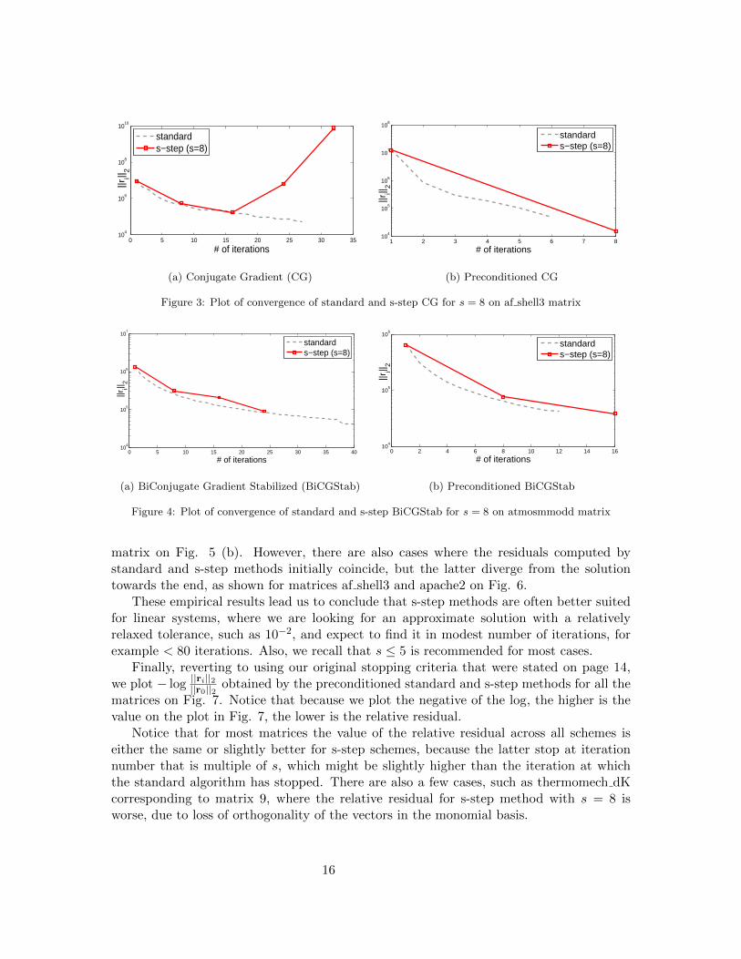
Second, let us make an important observation about numerical stability of s-step meth-ods. As we have mentioned earlier, the vectors in the monomial basis of the Krylov subspaceused in s-step methods can become linearly dependent relatively quickly. In fact, if we plot||ri||2 through iterations for s = 8 in red square, we can easily identify several occasionswhere these markings do not coincide with the grey line used for the standard scheme, seeFig. 3 and 4. Notice that in the case of s-step CG on Fig. 3 (a) the s-step method di-verged, while in the case of s-step BiCGStab on Fig 4 (a) the method exited early, becauseintermediate value ||s||2 fell below a specified threshold. This behavior is in line with theobservations made in [6] that for s > 5 s-step CG may suffer from loss of orthogonality andthat preconditioned s-step CG would likely fair better than its unpreconditioned version.

Third, let us look at the convergence of the preconditioned s-step iterative methodfor different stopping criteria. In particular, we are interested in what happens when weask the algorithm to achieve a tighter tolerance ||ri||2/||r0||2 < 10−7 and allow a largermaximum number of iterations. Notice that the residuals computed by the s-step methodsalways start following the ones computed by standard algorithms, see Fig 5 and 6. In somecases, the s-step methods match their standard counterparts exactly until the solution isfound, as shown for offshore matrix on Fig. 5 (a). In other cases, they follow the residualsapproximately, while still finding the solution towards the end, as shown for atmosmodd

15

0 5 10 15 20 25 30 3510

4

106

108

1010

# of iterations

||ri|| 2

standards−step (s=8)

(a) Conjugate Gradient (CG)

1 2 3 4 5 6 7 810

4

105

106

107

108

# of iterations

||ri|| 2

standards−step (s=8)

(b) Preconditioned CG

Figure 3: Plot of convergence of standard and s-step CG for s = 8 on af shell3 matrix

0 5 10 15 20 25 30 35 4010

4

105

106

107

# of iterations

||ri|| 2

standards−step (s=8)

(a) BiConjugate Gradient Stabilized (BiCGStab)

0 2 4 6 8 10 12 14 1610

4

105

106

# of iterations

||ri|| 2

standards−step (s=8)

(b) Preconditioned BiCGStab

Figure 4: Plot of convergence of standard and s-step BiCGStab for s = 8 on atmosmmodd matrix

matrix on Fig. 5 (b). However, there are also cases where the residuals computed bystandard and s-step methods initially coincide, but the latter diverge from the solutiontowards the end, as shown for matrices af shell3 and apache2 on Fig. 6.

These empirical results lead us to conclude that s-step methods are often better suitedfor linear systems, where we are looking for an approximate solution with a relativelyrelaxed tolerance, such as 10−2, and expect to find it in modest number of iterations, forexample < 80 iterations. Also, we recall that s ≤ 5 is recommended for most cases.

Finally, reverting to using our original stopping criteria that were stated on page 14,we plot − log ||ri||2||r0||2 obtained by the preconditioned standard and s-step methods for all thematrices on Fig. 7. Notice that because we plot the negative of the log, the higher is thevalue on the plot in Fig. 7, the lower is the relative residual.

Notice that for most matrices the value of the relative residual across all schemes iseither the same or slightly better for s-step schemes, because the latter stop at iterationnumber that is multiple of s, which might be slightly higher than the iteration at whichthe standard algorithm has stopped. There are also a few cases, such as thermomech dKcorresponding to matrix 9, where the relative residual for s-step method with s = 8 isworse, due to loss of orthogonality of the vectors in the monomial basis.

16

0 5 10 15 20 25 30

1010

1012

1014

# of iterations

||ri|| 2

standards−step (s=1)s−step (s=2)s−step (s=4)

(a) offshore

0 10 20 30 40 50 60 70 80

100

102

104

106

# of iterations

||ri|| 2

standards−step (s=1)s−step (s=2)s−step (s=4)

(b) atmosmodd

Figure 5: Plot of convergence of preconditioned methods for tighter tolerance ||ri||2/||r0||2 < 10−7

0 20 40 60 80 100 12010

2

104

106

108

1010

# of iterations

||ri|| 2

standards−step (s=1)s−step (s=2)s−step (s=4)

(a) af shell3 matrix

0 20 40 60 80 100 120

105

1010

1015

1020

1025

1030

# of iterations

||ri|| 2

standards−step (s=1)s−step (s=2)s−step (s=4)

(b) apache2 matrix

Figure 6: Plot of convergence of preconditioned methods for tighter tolerance ||ri||2/||r0||2 < 10−7

0

1

2

3

4

5

6

1 2 3 4 5 6 7 8 9 10 11 12

-lo

g(|

|r i

||

2/

||

r 0|

|2)

Matrix

(higher is better)

standard s=1 s=2 s=4 s=8

Figure 7: Plot of − log ||ri||2||r0||2obtained by preconditioned standard and s-step methods

17

The detailed results of the numerical experiments are shown in Tab. 2 and 3.

Standard s-step (s=1) s-step (s=2) s-step (s=4) s-step (s=8)

# # it.||ri||2||r0||2 # it.

||ri||2||r0||2 # it.

||ri||2||r0||2 # it.

||ri||2||r0||2 # it.

||ri||2||r0||2

1. 15 9.18E-03 15 9.18E-03 8 8.35E-03 4 8.35E-03 2 8.35E-032. 27 9.97E-03 27 9.96E-03 14 9.14E-03 7 9.13E-03 5 6.38E+063. 40 4.03E+00 40 4.03E+00 20 4.03E+00 10 4.03E+00 5 4.03E+004. 40 1.97E-01 40 1.97E-01 20 1.20E+06 10 1.51E+12 5 8.54E+045. 40 1.38E-01 40 1.38E-01 20 1.38E-01 10 1.38E-01 5 1.38E-016. 40 2.46E-02 40 2.46E-02 20 2.46E-02 10 2.46E-02 5 2.46E-027. 1 1.70E-03 1 1.70E-03 1 1.57E-03 1 1.37E-03 1 7.54E-048. 25.5 9.70E-03 26 9.70E-03 13 9.70E-03 7 9.70E-03 1 1.09E-019. 40 2.21E-01 40 1.79E-01 20 1.96E-01 1 1.78E-01 5 NaN10. 40 1.16E-02 40 3.47E-02 20 1.91E-02 1 1.69E-01 1 1.69E-0111. 1.5 2.67E-03 2 2.67E-03 1 2.67E-03 1 2.67E-03 1 2.67E-0312. 39.5 9.89E-03 39 9.41E-03 20 1.10E-02 10 1.14E-02 3 2.14E-02

Table 2: Results for standard and s-step unpreconditioned CG and BiCGStab methods

Standard s-step (s=1) s-step (s=2) s-step (s=4) s-step (s=8)

# # it.||ri||2||r0||2 # it.

||ri||2||r0||2 # it.

||ri||2||r0||2 # it.

||ri||2||r0||2 # it.

||ri||2||r0||2

1. 2 2.12E-03 2 2.12E-03 1 2.12E-03 1 1.23E-05 1 1.07E-062. 6 9.38E-03 6 9.38E-03 3 9.38E-03 2 2.95E-03 1 2.95E-033. 40 6.04E-01 40 6.04E-01 20 6.04E-01 10 6.04E-01 5 6.04E-014. 40 1.51E-01 40 7.85E-01 20 7.85E-01 10 7.85E-01 5 7.85E-015. 40 1.83E-02 40 1.85E-02 20 1.85E-02 10 1.85E-02 5 1.85E-026. 40 1.03E-02 40 1.03E-02 20 1.03E-02 10 1.03E-02 5 1.03E-027. 1 1.90E-04 1 1.90E-04 1 1.03E-04 1 8.58E-05 1 2.93E-058. 1.5 1.29E-03 2 1.29E-03 1 1.29E-03 1 1.29E-03 1 1.29E-039. 30 1.26E-01 40 1.44E-01 20 1.44E-01 10 1.44E-01 1 2.86E-0110. 0.5 5.63E-03 1 5.63E-03 1 5.63E-03 1 5.63E-03 1 5.63E-0311. 1 6.01E-04 1 6.01E-04 1 1.92E-05 1 1.92E-05 1 1.92E-0512. 11.5 9.87E-03 12 9.87E-03 6 9.87E-03 3 9.87E-03 2 9.04E-03

Table 3: Results for standard and s-step preconditioned CG and BiCGStab methods

18

5 Conclusion

In this paper we made an overview of the existing s-step CG iterative method and developeda novel s-step BiCGStab iterative method. We have also introduced preconditioning to boths-step algorithms, maintaining the extra work performed at each s iterations to the extramatrix-vector multiplication and a preconditioning solve.

We have discussed advantages of these methods, such as the use of matrix-power kerneland block dot-products, as well as their disadvantages, such as the loss of orthogonalityof the monomial Krylov subspace basis and extra work performed per iteration. Also, wehave pointed out the connection between s-step and communication-avoiding algorithms.

Finally, we performed numerical experiments to validate the theory behind the s-stepmethods, and will look at their performance in the future. These algorithms can potentiallybe a better alternative to their standard counterparts when modest tolerance and numberof iterations are required to solve a linear system on parallel platforms. Also, they could beused for a larger class of problems if the numerical stability issues related to the monomialbasis are resolved.

6 Acknowledgements

The author would like to acknowledge Erik Boman and Michael Garland for their usefulcomments and suggestions.

References

[1] R. Barrett, M. Berry, T. F. Chan, J. Demmel, J. Donato, J. Dongarra, V.Eijkhout, R. Pozo, C. Romine, H. van der Vorst, Templates for the Solutionof Linear Systems: Building Blocks for Iterative Methods, SIAM, Philadelphia, PA,1994.

[2] E. Carson, N. Knight and J. Demmel, Avoiding Communication in Nonsym-metric Lanczos-Based Krylov Subspace Methods, SIAM J. Sci. Comput., Vol. 35, pp.42-61, 2012.

[3] E. Carson, Communication-Avoiding Krylov Subspace Methods in Theory and Prac-tice, Ph.D. Thesis, University of California - Berkeley, 2015.

[4] A. T. Chronopoulos A Class of Parallel Iterative Methods on Multiprocessor, Ph.D.Thesis, University of Illinois - Urbana-Champagne, 1987.

[5] A. T. Chronopoulos, S-Step Iterative Methods for (Non)Symmetric (In)DefiniteLinear Systems, SIAM Journal on Numerical Analysis, Vol. 28, pp. 1776-1789, 1991.

19

[6] A. T. Chronopoulos and C. W. Gear, S-Step Iterative Methods for SymmetricLinear Systems, Journal of Computational and Applied Mathematics, Vol. 25, pp.153-168, 1989.

[7] A. T. Chronopoulos and C. D. Swanson, Parallel Iterative S-step Methods forUnsymmetric Linear Systems, Parallel Computing. Vol. 22, pp. 623-641, 1996.

[8] A. T. Chronopoulos and S. K. Kim, S-Step Orthomin and GMRES Implementedon Parallel Computers, Technical Report UMSI 90/43R, University of Minnesota Su-percomputing Institute, 1990.

[9] A. T. Chronopoulos and S. K. Kim, S-step Lanczos and Arnoldi Methods onParallel Computers, Technical Report UMSI 90/14R, University of Minnesota Super-computing Institute, Minneapolis, 1990.

[10] M. M. Dehnavi, J. Demmel, D. Giannacopoulos, Y. El-Kurdi,Communication-Avoiding Krylov Techniques on Graphics Processing Units, IEEETrans. on Magnetics, Vol. 49, pp. 1749-1752, 2013.

[11] A. El Guennouni, K. Jbilou and H. Sadok, A Block Version of BiCGStab forLinear Systems with Multiple Right-Hand-Sides, ETNA, 16, pp. 129–142 (2003).

[12] M. Hoemmen, Communication-Avoiding Krylov Subspace Methods, Ph.D. Thesis,University of California - Berkeley, 2010.

[13] M. Naumov, Parallel Incomplete-LU and Cholesky Factorization in the Precondi-tioned Iterative Methods on the GPU, Nvidia Technical Report, 3, 2012.

[14] M. Naumov, Preconditioned Block-Iterative Methods on GPUs, Proc. InternationalAssociation of Applied Mathematics and Mechanics, PAMM, Vol. 12, pp. 11-14, 2012.

[15] D. P. O’Leary, The Block Conjugate Gradient Algorithm and Related Methods, Lin-ear Algebra Appl., Vol. 29, pp. 293-322, 1980.

[16] J. van Rosendale, Minimizing Inner Product Data Dependence in Conjugate Gra-dient Iteration, Technical Report 172178, NASA Langley Research Center, 1983.

[17] Y. Saad, Iterative Methods for Sparse Linear Systems, SIAM, Philadelphia, PA, 2ndEd., 2003.

[18] I. Yamazaki, S. Rajamanickam, E. G. Boman, M. Hoemmen, M. A. Herouxand S. Tomov, Domain Decomposition Preconditioners for Communication-AvoidingKrylov Methods on Hybrid CPU/GPU Cluster, Proc. International Conference forHigh Performance Computing, Networking, Storage and Analysis, pp. 933-944, 2014.

[19] The University of Florida Sparse Matrix Collection (UFSMC),http://www.cise.ufl.edu/research/sparse/matrices/

20