S. J. Kim, T. S. Steenhuis - Cornell University

Transactions of the ASAEVol. 44(4): 863–875 � 2001 American Society of Agricultural Engineers ISSN 0001–2351 863

GRISTORM: GRID–BASED VARIABLE SOURCE

AREA STORM RUNOFF MODEL

S. J. Kim, T. S. Steenhuis

ABSTRACT. A grid–based storm runoff model in a variable source area is described. This model predicts temporal variationsand spatial distributions of subsurface flow–saturation overland flow with various shallow soil depths. The model usesASCII–formatted map data supported by the GRASS Geographic Information Systems (GIS) and generates distributed resultssuch as discharge, flow depth, and soil moisture in overland flow areas. The model uses a single overland flowpath algorithmand simulates surface and/or subsurface water depth at each grid element for a given time increment. A combinedsurface–subsurface kinematic modeling approach was used to simulate surface and subsurface flow. The model was appliedto a 170 ha watershed located in New York State. Predicted flows from six summer storm events in 1994 were compared withobserved flows at the watershed outlet. The initial soil moisture conditions for the storm events were based on calibratedvalues from Frankenberger’s Soil Moisture Routing (SMR) model and were adjusted to include soil moisture variations withina day. The average Nash–Sutcliffe efficiency for predicting runoff at the watershed outlet using calibrated parameters forthree storm events was 0.72. The initial soil moisture distribution proved to be the most sensitive parameter affecting streamflow at the watershed outlet and required calibration to obtain reasonable results. The second most sensitive parameter wasManning’s roughness coefficient for stream and overland areas. It affected the time and magnitude of peak stream flow. Resultsshowing temporal variations and spatial distributions of overland flow areas were presented using GRASS. According to theresults showing the spatial effect with differing grid element sizes, the model behavior was also sensitive to DEM gridresolution.

Keywords. Modeling, Grid–based, Storm runoff, Variable source area, GRASS, Geographic Information Systems.

hydrologic model that predicts surface andsubsurface flows and their flowpaths to the streamrequires the incorporation of throughflowprocesses in the GIS (Geographic Information

Systems) framework. Many catchment models have beenproposed, but few treat throughflow effectively. Severaldistributed physically based catchment models exist, such asSHE (Abbott et al., 1986), MIKE SHE (Refsgaard and Storm,1995), IHDM (Beven et al., 1987), and THALES (Grayson etal., 1992).

The source area for overland flow in a watershed shrinksand expands in response to rainfall in humid, well–vegetatedareas (Tischendorf, 1969; Dunne and Black, 1970; Hewlettand Nutter, 1970). The source area may be regarded as anexpansion of the perennial channel system into zones of lowstorage capacity fed from below by subsurface stormflow andfrom above by rainfall. During rainless periods, streams arefed largely by moisture migrating slowly downslope underconditions of unsaturated flow (Kirkby, 1978). As Dunne andBlack (1970) point out, the source area generates overland

Article was submitted for review in August 2000; approved forpublication by the Soil & Water Division of ASAE in April 2001.

The authors are Seong J. Kim, ASAE Member Engineer, AssistantProfessor, Department of Biological Systems Engineering, KonkukUniversity, Seoul, Korea; and Tammo S. Steenhuis, ASAE MemberEngineer, Professor, Department of Agricultural and BiologicalEngineering, Cornell University, Ithaca, New York. Correspondingauthor: Seong J. Kim, Department of Biological Systems Engineering,Konkuk University, Seoul 143–701, Korea; phone: +82–2–450–3749; fax:+82–2–444–0186; e–mail: [email protected].

flow, while the remainder of the watershed acts mainly as areservoir during storms to provide baseflow and to maintainthe wet areas that will produce subsequent storm runoff. Thisis especially true for well–vegetated watersheds in thenortheastern United States, in which shallow and slopingsoils predominate and for which the hydraulic conductivityof soils exceeds rainfall intensity by several fold (Kuo et al.,1999). A GIS can help to apportion storm runoff between thevarious flowpaths associated with source areas on slopes.

Recently, several researchers have attempted to model therainfall–runoff processes with GIS. GIS has proven to be anefficient tool for spatial analyses by visualizing the results ofhydrologic and water quality modeling. Allen (1987)developed SWHAM (Small Watershed Hydrologic AnalysisModel) using a GIS. This overland flow model is composedof a one–dimensional groundwater hydrologic model and astream flow model. Input data were extracted from soil, landuse/cover, and contour maps. Stuebe and Johnston (1990)applied GIS to all phases of the SCS (Soil ConservationService) modeling processes, including watersheddelineation and runoff routing, to estimate the outlet runoffvolume. Stuebe and Johnston’s work demonstrated the use ofGRASS to estimate runoff using the SCS runoff CurveNumber Model. Famiglietti (1992) used grid data extractedfrom a GIS to develop a model with grid–based water balanceand flow equations. Zollweg (1994) developed SMoRMod(Soil Moisture–based Runoff Model) using a series ofGRASS commands. The model is grid–based and composedof a daily soil moisture balance and sub–routines thatcalculate runoff generation and transport at 30–minuteintervals. The initial conditions for the runoff generation are

A

864 TRANSACTIONS OF THE ASAE

provided by the daily soil moisture balance. However, themodel has a tendency to over– or under–predict the recessionpart of hydrographs. Savabi et al. (1995) used GRASS toobtain the WEPP (Water Erosion Prediction Project) model’sinput parameters. Frankenberger (1996) and Franken–berger et al. (1999) modified Zollweg’s GIS–Based VariableSource Area Model using GRASS. The model, written inUNIX–shell script, predicts daily soil moisture and runoffbased on a water balance for shallow soils.

It is evident that during the past decade, distributedmodeling of surface and subsurface hydrology has becomecomputational, primarily because of the capability of GIS tohandle spatial data. Some studies have been conducted bycoupling GIS with distributed models within GIS software,called tight coupling (Stuart and Stocks, 1993). This is anembedded system where the GIS and models rely on a singledata manager. It makes the processes clear for the user tounderstand and modify for different conditions. On the otherhand, extensive progress has been made in managingdistributed models outside GIS, referred to as loose coupling(Goodchild, 1993; Nyerges, 1993). This makes the modelflexible and portable to another GIS software.

In this article, a grid–based subsurface and saturationoverland/stream flow generation procedure is described.This approach predicts the temporal variation and spatialdistribution of overland flow depth, discharge, and soilmoisture during a storm event. The applicability of theprocedure and its modification of the original surface andsubsurface kinematic modeling approach by Takasao andShiiba (1988) are also described. The model, coded inUNIX–C language, runs in GRASS (U.S. Army CERL, 1993)and uses regular gridded data such as elevation, stream, landuse, and soil information. The data used for this study werepreviously developed and described in Frankenberger(1996). The spatial results are displayed in GRASS.

MODEL DESCRIPTIONSATURATION OVERLAND/STREAM FLOW AND SUBSURFACEFLOW MODEL

Storm runoff in the northeastern United States, where theland surface is well vegetated, originates mainly fromsaturated areas (Dunne and Black, 1970). Saturated areasoften form where lateral subsurface flows converge, slopeschange, or where depth to the restricting layer decreases(Frankenberger, 1996). The amount of storm runoff isdirectly related to the magnitude of the saturated areas.

In order to model the formation of variable source areas,we adopted the combined surface–subsurface kinematicmodeling approach (Takasao and Shiiba, 1988). Thecontinuity equation applied to each grid element can bewritten as:

L

Q

L

rAQtA

c

c +=∂∂+

∂∂

�

�

� (1)

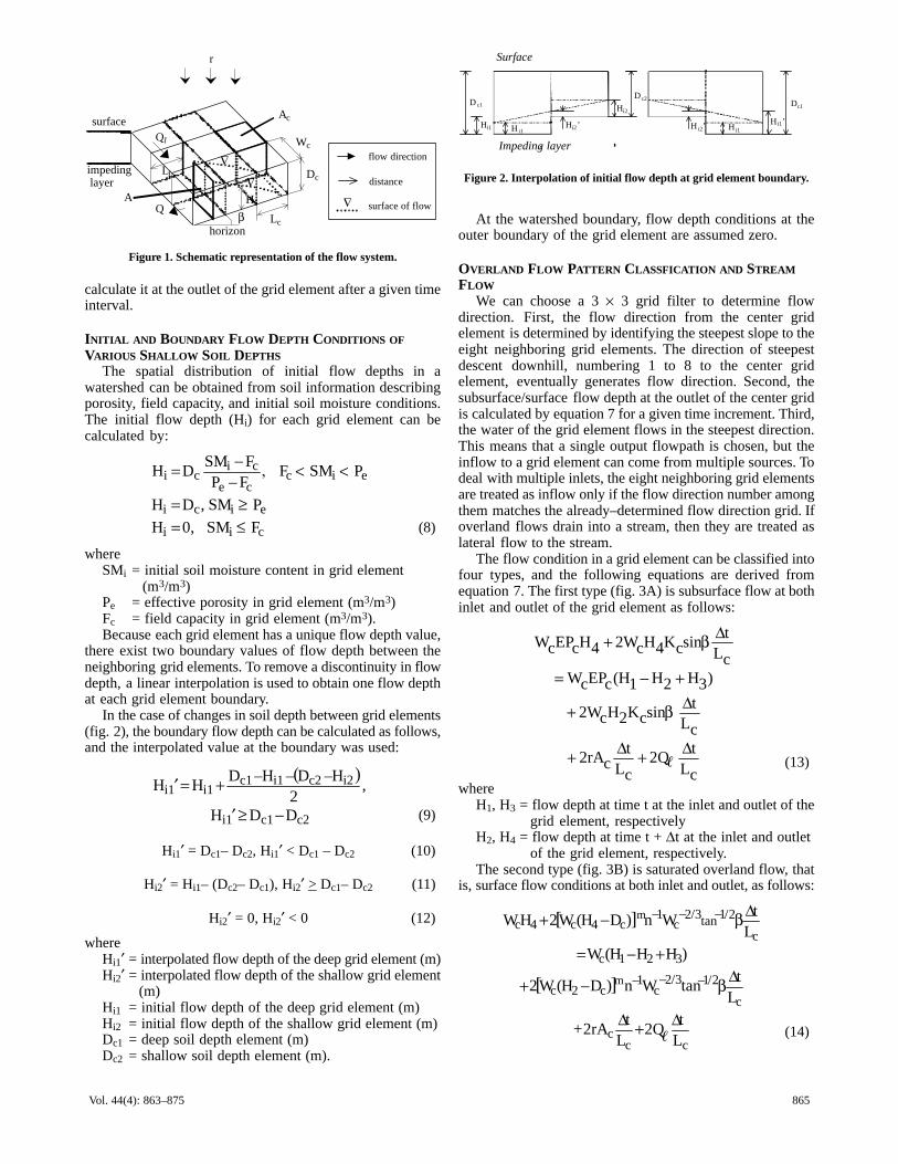
whereA = flow area (m2)Q = discharge (m3/sec)r = rainfall intensity (m/sec)Ac = grid element area of grid element c (m2)Lc = flow distance through the grid element c (m)

Q� = lateral discharge (m3/sec)

L� = lateral flow length (m)

t = time (sec)� = length (m).The flow areas for subsurface and saturation

overland/stream flow are:

A = Wc × EPc × H, 0 < H < Dc (2)

A = Wc × EPc × Dc + Af, H > Dc (3)

Af = Wc × (H – Dc) (4)

whereWc = grid element width orthogonal to streamline (m)EPc = total porosity minus field capacity (m3/m3)Dc = soil depth above the impeding layer (m)H = flow depth above the impeding layer (m)Af = overland flow area (m2).The resistance equation for subsurface flow, and the

kinematic wave equation for saturation overland/stream floware obtained by Darcy and Manning equations, respectively:

( )

( )sinKHW

DH0,sinEPA

KQ

ec

cc

e

××=

≤≤×= β

β (5)

Q = Wc × Dc × Kesin(β) + α Af m, H > Dc (6)

whereKe = saturated hydraulic conductivity (m/sec)β = grid element slope (degree)m = 5/3 for overland flow as shallow sheet flow (Rh = H)

and 4/3 for stream flowα = n–1 Wc –2/3 tan1/2β for overland flow and n–1 γ 2/3

tan1/2β for stream flown = Manning’s roughness coefficientγ = Rh Af

–1/2 (Moore and Foster, 1990; Moore and Burch,1986)

Rh = hydraulic radius.The schematic representation of the flow system is shown

in figure 1. The finite difference form of equation 1 isexpressed as:

ccc

c2

321c

44

L2Q

L2rA

L2Q

AAAL

2QA

+++

+−=+ �t

�t �t �t

� (7)

where∆t = time intervalA1, A3 = flow area at time t at the inlet and outlet of the

grid element, respectivelyA2, A4 = flow area at time t + ∆t at the inlet and outlet of

the grid element, respectivelyQ2, Q4 = discharge at time t + ∆t at the inlet and outlet of

the grid element, respectively.To solve equation 7, the four–point implicit scheme

developed by Brakensiek (1967) was adopted. The equationwas rearranged to solve for flow depth (H), and the Newton–Raphson method (Johnson and Riess, 1982) was used to

865Vol. 44(4): 863–875

r

surface

impeding layer

Q

Wc

Dc

Lchorizon

βH

Ql

Ll∇

flow direction

distance

∇ surface of flow

∇

A

Ac

Figure 1. Schematic representation of the flow system.

calculate it at the outlet of the grid element after a given timeinterval.

INITIAL AND BOUNDARY FLOW DEPTH CONDITIONS OF

VARIOUS SHALLOW SOIL DEPTHSThe spatial distribution of initial flow depths in a

watershed can be obtained from soil information describingporosity, field capacity, and initial soil moisture conditions.The initial flow depth (Hi) for each grid element can becalculated by:

cii

eici

eicce

cici

FSM0,H

PSM,DH

PSMFFPFSM

DH

≤=≥=

<<,−−=

(8)

whereSMi = initial soil moisture content in grid element

(m3/m3)Pe = effective porosity in grid element (m3/m3)Fc = field capacity in grid element (m3/m3).Because each grid element has a unique flow depth value,

there exist two boundary values of flow depth between theneighboring grid elements. To remove a discontinuity in flowdepth, a linear interpolation is used to obtain one flow depthat each grid element boundary.

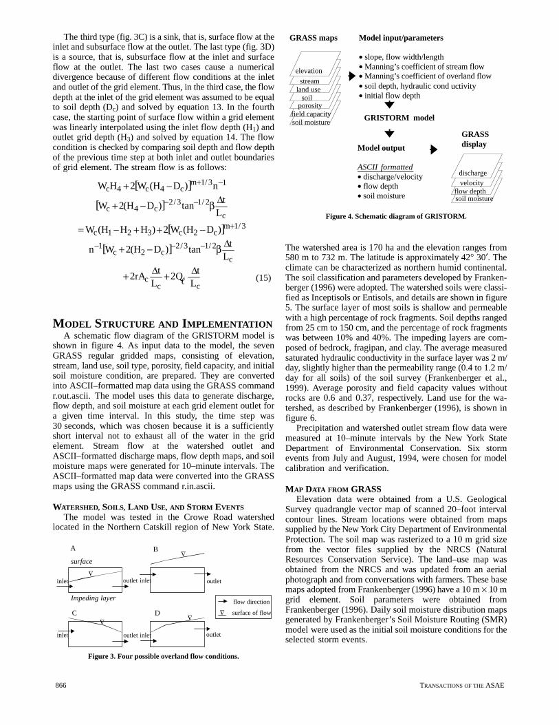
In the case of changes in soil depth between grid elements(fig. 2), the boundary flow depth can be calculated as follows,and the interpolated value at the boundary was used:

( )

c2c1i1

i2c2i1c1i1i1

DDH

,2

H–D–H–DHH

−≥′

+=′

(9)

Hi1′ = Dc1– Dc2, Hi1′ < Dc1 – Dc2 (10)

Hi2′ = Hi1– (Dc2– Dc1), Hi2′ > Dc1– Dc2 (11)

Hi2′ = 0, Hi2′ < 0 (12)

whereHi1′ = interpolated flow depth of the deep grid element (m)Hi2′ = interpolated flow depth of the shallow grid element

(m)Hi1 = initial flow depth of the deep grid element (m)Hi2 = initial flow depth of the shallow grid element (m)Dc1 = deep soil depth element (m)Dc2 = shallow soil depth element (m).

Surface

Impeding layerr

Dc2D c1

H i1

Hi2

Hi1’ Hi2’ H i2’Hi1’

Hi1

Dc1

Figure 2. Interpolation of initial flow depth at grid element boundary.

At the watershed boundary, flow depth conditions at theouter boundary of the grid element are assumed zero.

OVERLAND FLOW PATTERN CLASSFICATION AND STREAMFLOW

We can choose a 3 × 3 grid filter to determine flowdirection. First, the flow direction from the center gridelement is determined by identifying the steepest slope to theeight neighboring grid elements. The direction of steepestdescent downhill, numbering 1 to 8 to the center gridelement, eventually generates flow direction. Second, thesubsurface/surface flow depth at the outlet of the center gridis calculated by equation 7 for a given time increment. Third,the water of the grid element flows in the steepest direction.This means that a single output flowpath is chosen, but theinflow to a grid element can come from multiple sources. Todeal with multiple inlets, the eight neighboring grid elementsare treated as inflow only if the flow direction number amongthem matches the already–determined flow direction grid. Ifoverland flows drain into a stream, then they are treated aslateral flow to the stream.

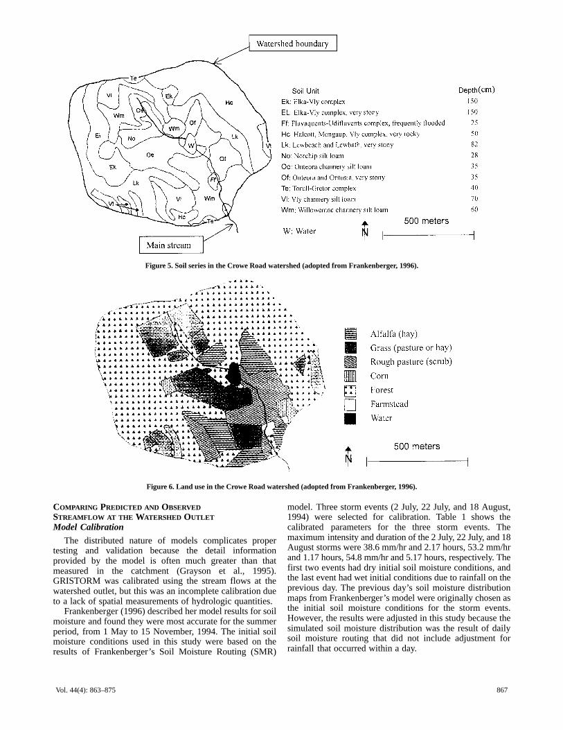
The flow condition in a grid element can be classified intofour types, and the following equations are derived fromequation 7. The first type (fig. 3A) is subsurface flow at bothinlet and outlet of the grid element as follows:

cLt

2QcLt

c2rA

cLt

sincK2Hc2W

)3H2H1H(cEPcWcLt

sincK4Hc2W4HcEPcW

∆+∆+

∆β+

+−=

∆β+

� (13)

whereH1, H3 = flow depth at time t at the inlet and outlet of the

grid element, respectivelyH2, H4 = flow depth at time t + ∆t at the inlet and outlet

of the grid element, respectively.The second type (fig. 3B) is saturated overland flow, that

is, surface flow conditions at both inlet and outlet, as follows:

[ ]

[ ]

ccc

c

2/13/2c

1mc2c

321c

c

2/1tan3/2c

1mc4c4c

Lt

2QL

t2rA+

Lt

tanWn)DH(W2

)HHH(WL

tWn)DH(W2HW

∆+∆

∆β−+

+−=

∆β−+

−−−

−−−

� (14)


The third type (fig. 3C) is a sink, that is, surface flow at theinlet and subsurface flow at the outlet. The last type (fig. 3D)is a source, that is, subsurface flow at the inlet and surfaceflow at the outlet. The last two cases cause a numericaldivergence because of different flow conditions at the inletand outlet of the grid element. Thus, in the third case, the flowdepth at the inlet of the grid element was assumed to be equalto soil depth (Dc) and solved by equation 13. In the fourthcase, the starting point of surface flow within a grid elementwas linearly interpolated using the inlet flow depth (H1) andoutlet grid depth (H3) and solved by equation 14. The flowcondition is checked by comparing soil depth and flow depthof the previous time step at both inlet and outlet boundariesof grid element. The stream flow is as follows:

[ ]

[ ]

[ ]

[ ]

ccc

c

2/13/2c2c

1

3/1mc2c321c

c

2/13/2c4c

13/1mc4c4c

Lt

2QL

t2rA

Lt

tan)DH(2Wn

)DH(W2)HHH(W

Lt

tan)DH(2W

n)DH(W2HW

∆+∆+

∆β−+

−++−=

∆β−+

−+

−−−

+

−−

−+

�(15)

MODEL STRUCTURE AND IMPLEMENTATIONA schematic flow diagram of the GRISTORM model is

shown in figure 4. As input data to the model, the sevenGRASS regular gridded maps, consisting of elevation,stream, land use, soil type, porosity, field capacity, and initialsoil moisture condition, are prepared. They are convertedinto ASCII–formatted map data using the GRASS commandr.out.ascii. The model uses this data to generate discharge,flow depth, and soil moisture at each grid element outlet fora given time interval. In this study, the time step was30 seconds, which was chosen because it is a sufficientlyshort interval not to exhaust all of the water in the gridelement. Stream flow at the watershed outlet andASCII–formatted discharge maps, flow depth maps, and soilmoisture maps were generated for 10–minute intervals. TheASCII–formatted map data were converted into the GRASSmaps using the GRASS command r.in.ascii.

WATERSHED, SOILS, LAND USE, AND STORM EVENTS

The model was tested in the Crowe Road watershedlocated in the Northern Catskill region of New York State.

flow direction

∇ surface of flow

A B

C D

outlet

surface

Impeding layer

∇

∇

∇ ∇

inlet inlet outlet

inlet outlet inlet outlet

Figure 3. Four possible overland flow conditions.

Model input/parameters

• slope, flow width/length• Manning’s coefficient of stream flow• Manning’s coefficient of overland flow• soil depth, hydraulic cond uctivity• initial flow depth

GRISTORM model

Model output

ASCII formatted• discharge/velocity• flow depth• soil moisture

dischargevelocity

flow depthsoil moisture

GRASSdisplay

elevation

streamland use

soilporosity

field capacitysoil moisture

GRASS maps

Figure 4. Schematic diagram of GRISTORM.

The watershed area is 170 ha and the elevation ranges from580 m to 732 m. The latitude is approximately 42° 30′. Theclimate can be characterized as northern humid continental.The soil classification and parameters developed by Franken-berger (1996) were adopted. The watershed soils were classi-fied as Inceptisols or Entisols, and details are shown in figure5. The surface layer of most soils is shallow and permeablewith a high percentage of rock fragments. Soil depths rangedfrom 25 cm to 150 cm, and the percentage of rock fragmentswas between 10% and 40%. The impeding layers are com-posed of bedrock, fragipan, and clay. The average measuredsaturated hydraulic conductivity in the surface layer was 2 m/day, slightly higher than the permeability range (0.4 to 1.2 m/day for all soils) of the soil survey (Frankenberger et al.,1999). Average porosity and field capacity values withoutrocks are 0.6 and 0.37, respectively. Land use for the wa-tershed, as described by Frankenberger (1996), is shown infigure 6.

Precipitation and watershed outlet stream flow data weremeasured at 10–minute intervals by the New York StateDepartment of Environmental Conservation. Six stormevents from July and August, 1994, were chosen for modelcalibration and verification.

MAP DATA FROM GRASSElevation data were obtained from a U.S. Geological

Survey quadrangle vector map of scanned 20–foot intervalcontour lines. Stream locations were obtained from mapssupplied by the New York City Department of EnvironmentalProtection. The soil map was rasterized to a 10 m grid sizefrom the vector files supplied by the NRCS (NaturalResources Conservation Service). The land–use map wasobtained from the NRCS and was updated from an aerialphotograph and from conversations with farmers. These basemaps adopted from Frankenberger (1996) have a 10 m × 10 mgrid element. Soil parameters were obtained fromFrankenberger (1996). Daily soil moisture distribution mapsgenerated by Frankenberger’s Soil Moisture Routing (SMR)model were used as the initial soil moisture conditions for theselected storm events.

867Vol. 44(4): 863–875

Figure 5. Soil series in the Crowe Road watershed (adopted from Frankenberger, 1996).

Figure 6. Land use in the Crowe Road watershed (adopted from Frankenberger, 1996).

COMPARING PREDICTED AND OBSERVED STREAMFLOW AT THE WATERSHED OUTLET

Model Calibration

The distributed nature of models complicates propertesting and validation because the detail informationprovided by the model is often much greater than thatmeasured in the catchment (Grayson et al., 1995).GRISTORM was calibrated using the stream flows at thewatershed outlet, but this was an incomplete calibration dueto a lack of spatial measurements of hydrologic quantities.

Frankenberger (1996) described her model results for soilmoisture and found they were most accurate for the summerperiod, from 1 May to 15 November, 1994. The initial soilmoisture conditions used in this study were based on theresults of Frankenberger’s Soil Moisture Routing (SMR)

model. Three storm events (2 July, 22 July, and 18 August,1994) were selected for calibration. Table 1 shows thecalibrated parameters for the three storm events. Themaximum intensity and duration of the 2 July, 22 July, and 18August storms were 38.6 mm/hr and 2.17 hours, 53.2 mm/hrand 1.17 hours, 54.8 mm/hr and 5.17 hours, respectively. Thefirst two events had dry initial soil moisture conditions, andthe last event had wet initial conditions due to rainfall on theprevious day. The previous day’s soil moisture distributionmaps from Frankenberger’s model were originally chosen asthe initial soil moisture conditions for the storm events.However, the results were adjusted in this study because thesimulated soil moisture distribution was the result of dailysoil moisture routing that did not include adjustment forrainfall that occurred within a day.


Table 1. Summary of model calibration and its parameters.

TotalManning’s n

HydraulicConductivity

(m/day)[a]

Initial SoilMoisture

Adjustment Ratio Total Runoff Peak Discharge3

StormTotal

Rainfall Grass/ Farm– High Low Silt

Total Runoff(mm)

Peak Discharge(m3/s)

StormEvent

Rainfall(mm) Stream Forest

Grass/Alfalfa Corn

Farm–stead

HighSMA

LowSMA Stony

SiltLoam Obs. Pre. Obs. Pre.

2 July 94 24.02 0.03 0.15 0.14 0.17 0.09 1.20 0.80 1.066 1.072 1.72 1.64 0.234 0.235

22 July 94 24.76 0.02 0.26 0.20 0.23 0.12 2.00 0.80 0.520 0.560 1.17 1.00 0.236 0.23018 Aug 94 22.62 0.04 0.20 0.14 0.17 0.09 1.20 0.80 0.610 0.690 5.99 5.54 0.276 0.267Mean 23.80 0.03 0.20 0.16 0.19 0.10 1.47 0.80 0.732 0.774 2.96 2.73 0.249 0.244[a] SMA = Soil Moisture Area.

To simplify the calibration, the adjustment of initial soilmoisture conditions was accomplished by categorizing thewatershed’s 11 soil types into 2 groups: stony and silt loam.A constant initial soil moisture adjustment factor wasmultiplied by the digital numbers of Frankenberger’s soilmoisture distribution map. The factor ranged from 0.520 forstony soils during the 22 July storm to 1.072 for silt loam soilsduring the 2 July storm, as shown in table 1. To applyManning’s equation in this study, the pond in the middle ofthe watershed was simply treated as a stream having verygentle slopes.

Figure 7 shows the observed versus predicted stream flowat the watershed outlet for the 2 July storm. The predictedrunoff agreed well with the observed values, but the totalrunoff was underestimated for the three events, assummarized in table 1. Predicted runoff decreased rapidly atthe falling limb for the 22 July and 18 August storms, but itdecreased slowly at the baseflow recession for all stormevents. This error may be caused by the scale–basedparameterization of grid element processes with theundefined complexity of local heterogeneity andsimplification of subsurface flow representation in themodel. Preferential flow through macropores in the soil cancontribute to stream flow as a subsurface lateral flow. Othersources of error may arise from the uncertainty of initial soilmoisture condition and lumped parameters within each 10 m× 10 m grid element.

Sensitivity Analysis

To examine the effect of model parameters on simulationoutput, sensitivity analysis was conducted for the 2 Julystorm. The calibrated parameters [Manning’s roughnesscoefficients (MRC), hydraulic conductivity (HC), and initialsoil moisture adjustment ratio (ISMAR)] from table 1 wereused as base values. Figure 8 shows the simulated stream flowat the watershed outlet with varying values of a target param–

0.00

0.05

0.10

0.15

0.20

0.25

0.30

Dis

char

ge (

m^3

/sec

)

0

20

40

60

80

100

120

Rai

nfal

l (m

m/h

r)

23.5 0.00 0.50 1.00 1.50 2.00 2.50 3.00 3.50 4.00

Time (hours)

Observed Predicted

July 2, 1994

Figure 7. Comparison of predicted and observed stream flow for the 2July storm.

eter, while keeping other parameters at the base value. Thevalues in the legends are the multiplication ratios for the cor-responding parameters.

Initial soil moisture distribution before a storm event(fig. 8C) proved to be the most sensitive parameter affectingthe magnitude of peak discharge and total runoff within thecapacity of soil moisture. The peak discharges for 0.9, 1.0,1.05, 1.10, and 1.25 ISMAR were 0.170, 0.235, 0.828, 0.993,and 1.019 m3/sec, and the total runoff was 0.67, 1.64, 5.35,6.09, and 6.29 mm, respectively. Manning’s roughnesscoefficients for stream, forest, and grass/alfalfa were thesecond most sensitive parameters. The time of peakdischarge moved from 0:40 hr to 1:24 hr as MRC of streamincreased (fig. 8A). The peak discharges for 0.5, 0.75, 1.0,1.5, and 2.0 MRC were 0.322, 0.268, 0.235, 0.262, and0.263 m3/sec, and the total runoff was 1.70, 1.63, 1.64, 1.55,and 1.52 mm, respectively.

MRC for forest and grass/alfalfa affected the magnitudeof peak discharge and total runoff the most. The time of peakdischarge moved from 1:04 hr to 0:24 hr as MRC of forestincreased. The peak discharges for 0.5, 0.75, 1.0, 1.5, and2.0 MRC of forest were 0.363, 0.275, 0.235, 0.241, and0.237 m3/sec, and the total runoff was 2.20, 1.81, 1.64, 1.54,and 1.42 mm, respectively. The discharge decreased as MRCfor forest increased. The peak discharges for 0.5, 0.75, 1.0,1.5, and 2.0 MRC of grass/alfalfa were 0.236, 0.225, 0.235,0.300, and 0.337 m3/sec, and the total runoff was 1.76, 1.64,1.64, 1.83, and 1.96 mm, respectively.

Note that the discharge increased as MRC for grass/alfalfaincreased. Because this area is near the stream and has highinitial soil moisture contents, the condition of overland flowis reached rapidly and drained to the stream without causinga time lag. MRC for corn and farmstead also affected theshape of the hydrograph depending on the areal portion ofwatershed.

Saturated hydraulic conductivity had little effectcompared with other parameters (fig. 8B). This is due to thetime scale of a storm event. Subsurface lateral flow should bea key component for long–term soil moisture routing in thewater balance, but not for short–term storm runoffsimulation. From the results of sensitivity analysis, we canconclude that ISMAR estimates water balance for the stormevent to some extent, and then MRC and HC influence thepeak time and rising and falling limbs of the hydrograph.

Model Verification

The model was verified using the average value ofcalibrated parameters from table 1 (except the initial soilmoisture adjustment factor, which differs for each

869Vol. 44(4): 863–875

0

0.1

0.2

0.3

0.4

Dis

char

ge (

m^3

/sec

)

23.5 0.00 0.50 1.00 1.50 2.00 2.50 3.00 3.50 4.00Time (hours)

0.5 0.75 1.0 1.5 2.0

Manning’s n (Stream)A

0

0.1

0.2

0.3

0.4

Dis

char

ge (

m^3

/sec

)

23.5 0.00 0.50 1.00 1.50 2.00 2.50 3.00 3.50 4.00Time (hours)

1 3 5 10 100

Hydraulic Conductivity

B

0

0.3

0.6

0.9

1.2

Dis

char

ge (

m^3

/sec

)

23.5 0.00 0.50 1.00 1.50 2.00 2.50 3.00 3.50 4.00Time (hours)

0.9 1.0 1.05 1.1 1.25ISMARC

Figure 8. Parameter sensitivity of Manning’s roughness coefficients, saturated hydraulic conductivity, and initial soil moisture distribution for the 2July storm.

storm–event/soil–group combination) to predict streamflows at the watershed outlet for three other summer storms(14 August, 17 August, and 21 August, 1994). The maximumintensity and duration of the 14 August, 17 August, and21 August storms were 35.3 mm/hr and 9.17 hours, 8.2 mm/hr and 5.33 hours, and 40.1 mm/hr and 2.0 hours, respective-ly. The adjustment factor for initial soil moisture ranged from1.066 for stony soil during the 21 August storm, to 1.230 forsilt loam soil during the 14 August storm. The predicted out-

let stream flows for the three storms were compared with ob-served values. Figure 9 shows the observed versus predictedstream flow at the watershed outlet for the 14 August storm.A summary of model verification is given in table 2. The av-erage Nash–Sutcliffe efficiency R2 (Nash and Sutcliffe,1970) for the model was 0.72. Despite the verification of themodel, many sources of uncertainty exist in the predictionsof the variable source area storm runoff model. Beven andBinley (1992) listed other potential sources of error in


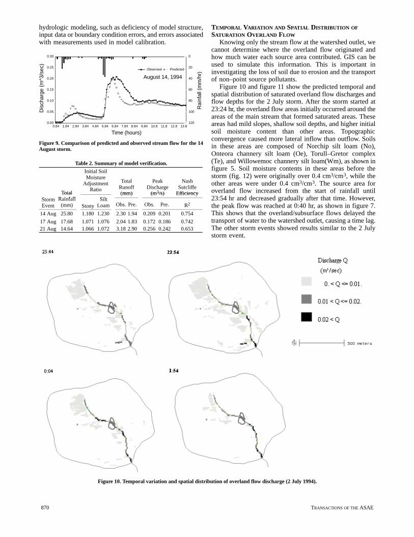
hydrologic modeling, such as deficiency of model structure,input data or boundary condition errors, and errors associatedwith measurements used in model calibration.

0.00

0.05

0.10

0.15

0.20

0.25

0.30

Dis

char

ge (

m^3

/sec

)

0

20

40

60

80

100

120

Rai

nfal

l (m

m/h

r)

0.84 1.84 2.84 3.84 4.84 5.84 6.84 7.84 8.84 9.84 10.8 11.8 12.8 13.8

Time (hours)

Observed Predicted

August 14, 1994

Figure 9. Comparison of predicted and observed stream flow for the 14August storm.

Table 2. Summary of model verification.

Total

Initial SoilMoisture

AdjustmentRatio

TotalRunoff(mm)

PeakDischarge

(m3/s)

NashSutcliffe

EfficiencyStorm

TotalRainfall Silt

(mm) (m3/s) EfficiencyStormEvent

TotalRainfall(mm) Stony

SiltLoam Obs. Pre. Obs. Pre. R2

14 Aug 25.80 1.180 1.230 2.30 1.94 0.209 0.201 0.754

17 Aug 17.68 1.071 1.076 2.04 1.83 0.172 0.186 0.74221 Aug 14.64 1.066 1.072 3.18 2.90 0.256 0.242 0.653

TEMPORAL VARIATION AND SPATIAL DISTRIBUTION OFSATURATION OVERLAND FLOW

Knowing only the stream flow at the watershed outlet, wecannot determine where the overland flow originated andhow much water each source area contributed. GIS can beused to simulate this information. This is important ininvestigating the loss of soil due to erosion and the transportof non–point source pollutants.

Figure 10 and figure 11 show the predicted temporal andspatial distribution of saturated overland flow discharges andflow depths for the 2 July storm. After the storm started at23:24 hr, the overland flow areas initially occurred around theareas of the main stream that formed saturated areas. Theseareas had mild slopes, shallow soil depths, and higher initialsoil moisture content than other areas. Topographicconvergence caused more lateral inflow than outflow. Soilsin these areas are composed of Norchip silt loam (No),Onteora channery silt loam (Oe), Torull–Gretor complex(Te), and Willowemoc channery silt loam(Wm), as shown infigure 5. Soil moisture contents in these areas before thestorm (fig. 12) were originally over 0.4 cm3/cm3, while theother areas were under 0.4 cm3/cm3. The source area foroverland flow increased from the start of rainfall until23:54 hr and decreased gradually after that time. However,the peak flow was reached at 0:40 hr, as shown in figure 7.This shows that the overland/subsurface flows delayed thetransport of water to the watershed outlet, causing a time lag.The other storm events showed results similar to the 2 Julystorm event.

Figure 10. Temporal variation and spatial distribution of overland flow discharge (2 July 1994).

871Vol. 44(4): 863–875

Figure 11. Temporal variation and spatial distribution of overland flow depth (2 July 1994).

Figure 12. Spatial distribution of soil moisture before and after rainfall (2 July 1994).

SPATIAL EFFECT OF CHANGING GRID ELEMENT SIZEQuinn et al. (1995) described the importance of grid

resolution for the validation of spatial model prediction.They discussed the effect of the grid element size on theTOPMODEL (Beven and Kirkby, 1979) parameter,ln(a/tanβ) and model results. Refsgaard (1997) suggested themethodologies for the validation of new distributed models.He mentioned that multi–site runoff, soil moisture, orgroundwater heads in a watershed should be measured andcompared with the simulated ones for successful modelvalidation. Even though this study did not sufficiently fulfillthe distributed model’s verification requirements in themanner of spatial verification, temporal calibration andverification with six storm events was performed by grouping

and adjusting saturated hydraulic conductivity and initial soilmoisture content.

A spatial test of the model behavior by changing gridelement size to 20, 30, and 40 m was conducted. In spatialaggregation, the values of the grid elements for continuousdata, such as digital elevation models (DEMs) and three soilparameters, were averaged, while the most common value ofthe grid elements was selected for categorical data, such assoil, land use, and stream. New DEMs for 10, 20, 30, and40 m grid elements are shown in figure 13A, B, C, and D,respectively. The slope distribution for each DEM is shownin figure 14A, B, C, and D. The average slopes were 8.11°,7.81°, 7.76°, and 8.15°, respectively. The results show thedeterioration of slope distribution and the losses of boundary


N 500 meters

Figure 13. New DEMs for grid element size: (A) 10 m, (B) 20 m, (C) 30 m, and (D) 40 m.

Figure 14. Slope distribution for each DEM: (A) 10 m, (B) 20 m, (C) 30 m, and (D) 40 m.

873Vol. 44(4): 863–875

information with increasing grid element size. Recently,Kuo et al. (1999) suggested a new spatial aggregation meth-od for border cells to conserve information inside the trueboundary by considering the proportion of the border cell thatis within the watershed. Model errors introduced by aggrega-tion of spatial data may be reduced if the method by Kuo etal. (1999) is adopted. Because this study is not focused on thescaling effect toward macroscale hydrological modeling, theadjustment for border cells was not included.

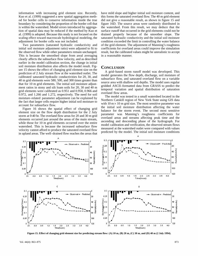
Two parameters (saturated hydraulic conductivity andinitial soil moisture adjustment ratio) were adjusted to fit tothe observed flow while other parameters remain unchanged.This is because the smoothed slope from areal averagingclearly affects the subsurface flow velocity, and as describedearlier in the model calibration section, the change in initialsoil moisture distribution also affects the model result. Fig-ure 15 shows the effect of changing grid element size on theprediction of 2 July stream flow at the watershed outlet. Thecalibrated saturated hydraulic conductivities for 20, 30, and40 m grid elements were 580, 500, and 300 times greater thanthat for 10 m grid elements. The initial soil moisture adjust-ment ratios in stony and silt loam soils for 20, 30 and 40 mgrid elements were calibrated as 0.951 and 0.958, 0.966 and0.972, and 1.266 and 1.272, respectively. The need for soilmoisture–related parameter adjustment can be explained bythe fact that larger cells require higher initial soil moisture toaccount for subsurface flow.

Figure 16 shows the spatial effect of changing gridelement size on the flow depth distribution for the 2 Julystorm at 0:40 hr. The overland flow areas for 20 and 30 m gridelements occurred just around the areas of the main stream,while those for 10 m grid elements occurred over the entirewatershed. This is because the increased subsurface flowvelocity cannot afford to produce the saturated overland flowin upland areas. The well–drained flow reaches the areas that

have mild slope and higher initial soil moisture content, andthis forms the saturated overland flow. The 40 m grid elementdid not give a reasonable result, as shown in figure 15 andfigure 16D. The source areas were randomly distributed inthe watershed. From this result, we may deduce that thesurface runoff that occurred in the grid elements could not bedrained properly because of the smoother slope. Thesaturated hydraulic conductivity and the initial soil moisturecondition exceeded the limit in controlling the water balanceof the grid element. The adjustment of Manning’s roughnesscoefficients for overland areas could improve the simulationresult, but the calibrated values might be unrealistic to acceptin a reasonable manner.

CONCLUSIONA grid–based storm runoff model was developed. This

model generates the flow depth, discharge, soil moisture ofsubsurface flow, and saturated overland flow on a variablesource area with shallow soil depths. The model uses regulargridded ASCII–formatted data from GRASS to predict thetemporal variation and spatial distribution of saturationoverland flow areas.

The model was tested in a small watershed located in theNorthern Catskill region of New York State using GIS datawith 10 m × 10 m grid size. The most sensitive parameter wasthe initial soil moisture distribution affecting the waterbalance for the storm event. The second most sensitiveparameter was Manning’s roughness coefficients foroverland areas and streams affecting peak time and theascending and descending phase of the hydrograph. Formodel calibration and verification, the observed stream flowsmeasured at the watershed outlet were compared with valuespredicted by the model. The initial soil moisture conditions

Figure 15. Effect of changing grid element size for predicting stream flow: (A) 10 m, (B) 20 m, (C) 30 m, and (D) 40 m (2 July 1994).


Figure 16. Spatial effect of changing grid element size for the 2 July storm at 0:40 hr represented by overland flow depth: (A) 10 m, (B) 20 m, (C) 30 m,and (D) 40 m.

for the storm events were adopted from the previous day’ssoil moisture distribution maps by Frankenberger’s SMRmodel (Frankenberger, 1996). These were recalibrated byintroducing adjustment factors for two soil types (stony andsilt loam). The spatial distributions of saturated overlandflow areas for several storm events were modeled and dis-played with GRASS. The calculated overland flow areas oc-curred around the areas of the main stream that had highinitial soil moisture contents. Temporal variation in thoseareas showed that the overland/subsurface flows attenuateand cause lag in stream flows. Finally, spatial testing wasconducted by changing grid resolution to 20, 30, and 40 m.The model behavior was sensitive to DEM grid resolution.Increasing the grid element size deteriorated the slopedistribution and lost the boundary information. This requiredparameter adjustment of saturated hydraulic conductivityand initial soil moisture adjustment ratio to obtain reasonableresults.

ACKNOWLEDGEMENTS

The authors thank Dr. Jane Frankenberger of theDepartment of Agricultural and Biological Engineering,Purdue University, and Dr. Jan Boll of the Department ofBiological and Agricultural Engineering, University ofIdaho, for providing GIS and field data and for discussionsthat aided in the preparation of this article. Many thanks mustbe given to Dr. Mark Risse and the anonymous reviewers whoimproved earlier versions of this article. Thanks also go toDr. Soon–Jin Hwang, who read proofs with religious care.

REFERENCESAbbott, M. B., J. C. Bathurst, J. O. Cunge, P. E. O’Connell, and J.

Rasmussen. 1986. An introduction to the European hydrological

system: Systeme Hydrologique Europeen (SHE). J. Hydrology87(1): 45–59.

Allen, S. J. 1987. Digital hydrologic modeling methods for waterresources engineering with application to the Broad Brookwatershed. Ph.D. dissertation. The University of Connecticut,Storrs, Conn.

Beven, K. J., and A. Binley. 1992. The future of distributed models:Model calibration and uncertainty prediction. Hydrol. Process.6(3): 279–298.

Beven, K. J., A. Calver, and E. M. Morris. 1987. The Institute ofHydrology Distributed Model. Report 98. Wallingford, U.K.:The Institute of Hydrology.

Beven, K. J., and M. J. Kirkby. 1979. A physically–based variablecontributing area model of basin hydrology. Hydrologic Sci.Bull. 24(1): 43–69.

Brakensiek, D. L. 1967. Kinematic flood routing. Trans.ASAE10(3): 340–343.

Dunne, T., and R. D. Black. 1970. Partial area contributions tostorm runoff in a small New England watershed. WaterResources Res. 6(5): 1296–1311.

Famiglietti, J. S. 1992. Aggregation and scaling ofspatially–variable hydrological process: Local catchment–scaleand macroscale models of water and energy balance. Ph.D.dissertation. University of Maryland, College Park, Md.

Frankenberger, J. R. 1996. Identification of critical runoffgenerating areas using a variable source area model. Ph.D.dissertation. Cornell University, Ithaca, N.Y.

Frankenberger, J. R., E. S. Brooks, M. T. Walter, M. F. Walter, andT. S. Steenhuis. 1999. A GIS–based variable source areahydrology model. Hydrol. Process. 13(6): 805–822.

Goodchild, M. F. 1993. The state of GIS for environmentalproblem–solving. In Environmental Modeling with GIS, 8–15.M. F. Goodchild, B. O. Parks, and L. T. Steyaert, eds. New York,N.Y.: Oxford University Press.

Grayson, R. B., I. D. Moore, and T. A. McMahon. 1992. Physicallybased hydrological modeling. 1. A terrain–based model forinvestigative purposes. Water Resources Res. 28(10):2659–2666.

875Vol. 44(4): 863–875

Grayson, R. B., G. Blöschl, and I. D. Moore. 1995. Distributedparameter hydrologic modeling using vector elevation data:THALES and TAPES–C. In Computer Models of WatershedHydrology, 669–696. V. P. Singh, ed. Highlands Ranch, Colo.:Water Resources Publications.

Hewlett, J. D., and W. L. Nutter. 1970. The varying source area ofstreamflow from upland basins. In Proc. Symposium onInterdisciplinary Aspects of Watershed Management, 65–83.Bozeman, Mont.: Montana State University. St. Joseph, Mich.:ASAE.

Johnson, L. W., and R. D. Riess. 1982. Solution of nonlinearequations. In Numerical Analysis, 160–164. Boston, Mass.:Addison–Wesley.

Kirkby, M. J. 1978. The hillslope hydrological cycle. In HillslopeHydrology, 31. M. J. Kirkby, ed. Chichester, U.K.: John Wiley.

Kuo, W.–L., T. S. Steenhuis, C. E. McCulloch, C. L. Mohler, D. A.Weinstein, S. D. DeGloria, and D. P. Swaney. 1999. Effect ofgrid size on runoff and soil moisture for a variable–source–areahydrology model. Water Resources Res. 35(11): 3419–3428.

Moore, I. D., and G. J. Burch. 1986. Sediment transport capacity ofsheet and rill flow: Application of unit stream power theory.Water Resources Res. 22(8): 1350–1360.

Moore, I. D., and G. R. Foster. 1990. Hydraulics and overland flow.In Process Studies in Hillslope Hydrology, 215–254. M. G.Anderson and T. P. Burt, eds. New York, N.Y.: John Wiley.

Nash, J. E., and J. V. Sutcliffe. 1970. River flow forecasting throughconceptual models: Part I. A discussion of principles. J.Hydrology 10(3): 283–290.

Nyerges, T. L. 1993. Understanding the scope of GIS: Itsrelationship to environmental modeling. In EnvironmentalModeling with GIS, 75–93. M. F. Goodchild, B. O. Parks, andL. T. Steyaert, eds. New York, N.Y.: Oxford University Press.

Quinn, P. F., K. J. Beven, and R. Lamb. 1995. The ln(a/tanβ) index:How to calculate it and how to use it within the TOPMODELframework. Hydrol. Process. 9(2): 161–182.

S. J. Kim, T. S. Steenhuis - Cornell University

Documents

Transcript of S. J. Kim, T. S. Steenhuis - Cornell University