
S-Frame Day 1 - Standard - April 2012 (Electronic)
180
For support and training on the full range of CSC products, please contact… Support: [email protected] Training: [email protected] Training manual Standard
description
Engineering
Transcript of S-Frame Day 1 - Standard - April 2012 (Electronic)

For support and training on the full range of CSC products, please contact…
Support: [email protected]
Training: [email protected]
Training manualStandard
1 2012 Version 10.0 April
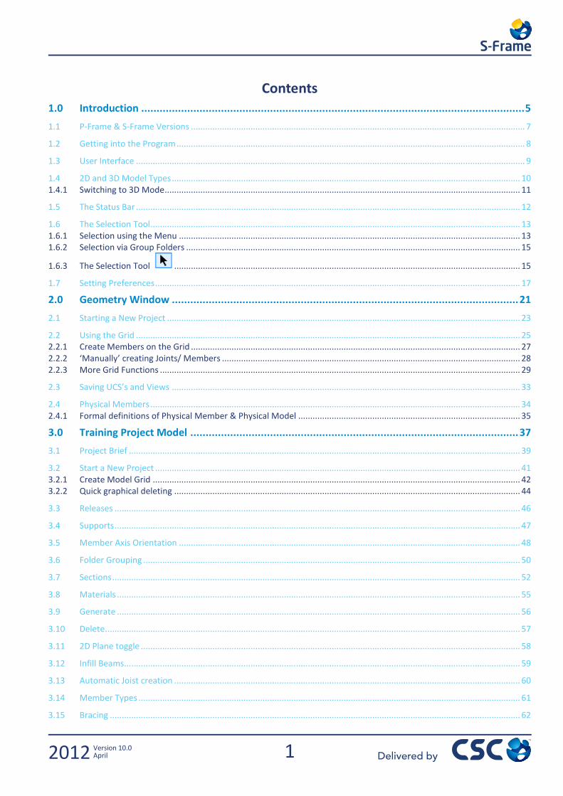
Contents 1.0 Introduction ............................................................................................................................. 5
1.1 P-Frame & S-Frame Versions ............................................................................................................................................ 7
1.2 Getting into the Program .................................................................................................................................................. 8
1.3 User Interface ................................................................................................................................................................... 9
1.4 2D and 3D Model Types .................................................................................................................................................. 10 1.4.1 Switching to 3D Mode ..................................................................................................................................................... 11
1.5 The Status Bar ................................................................................................................................................................. 12
1.6 The Selection Tool ........................................................................................................................................................... 13 1.6.1 Selection using the Menu ............................................................................................................................................... 13 1.6.2 Selection via Group Folders ............................................................................................................................................ 15
1.6.3 The Selection Tool ................................................................................................................................................. 15
1.7 Setting Preferences ......................................................................................................................................................... 17
2.0 Geometry Window ................................................................................................................. 21
2.1 Starting a New Project .................................................................................................................................................... 23
2.2 Using the Grid ................................................................................................................................................................. 25 2.2.1 Create Members on the Grid .......................................................................................................................................... 27 2.2.2 ‘Manually’ creating Joints/ Members ............................................................................................................................. 28 2.2.3 More Grid Functions ....................................................................................................................................................... 29
2.3 Saving UCS’s and Views .................................................................................................................................................. 33
2.4 Physical Members ........................................................................................................................................................... 34 2.4.1 Formal definitions of Physical Member & Physical Model ............................................................................................. 35
3.0 Training Project Model ........................................................................................................... 37
3.1 Project Brief .................................................................................................................................................................... 39
3.2 Start a New Project ......................................................................................................................................................... 41 3.2.1 Create Model Grid .......................................................................................................................................................... 42 3.2.2 Quick graphical deleting ................................................................................................................................................. 44
3.3 Releases .......................................................................................................................................................................... 46
3.4 Supports .......................................................................................................................................................................... 47
3.5 Member Axis Orientation ............................................................................................................................................... 48
3.6 Folder Grouping .............................................................................................................................................................. 50
3.7 Sections ........................................................................................................................................................................... 52
3.8 Materials ......................................................................................................................................................................... 55
3.9 Generate ......................................................................................................................................................................... 56
3.10 Delete .............................................................................................................................................................................. 57
3.11 2D Plane toggle ............................................................................................................................................................... 58
3.12 Infill Beams...................................................................................................................................................................... 59
3.13 Automatic Joist creation ................................................................................................................................................. 60
3.14 Member Types ................................................................................................................................................................ 61
3.15 Bracing ............................................................................................................................................................................ 62
2 2012 Version 10.0 April
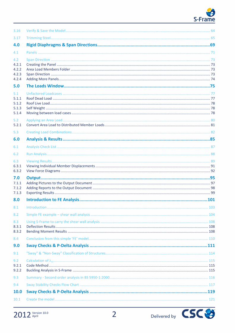
3.16 Verify & Save the Model ................................................................................................................................................. 64
3.17 Trimming Steel ................................................................................................................................................................ 65
4.0 Rigid Diaphragms & Span Directions ........................................................................................ 69
4.1 Panels ............................................................................................................................................................................. 71
4.2 Span Direction ................................................................................................................................................................ 73 4.2.1 Creating the Panel .......................................................................................................................................................... 73 4.2.2 Area Load Members Folder ............................................................................................................................................ 73 4.2.3 Span Direction ................................................................................................................................................................ 73 4.2.4 Adding More Panels........................................................................................................................................................ 74
5.0 The Loads Window .................................................................................................................. 75
5.1 Unfactored Loadcases .................................................................................................................................................... 77 5.1.1 Roof Dead Load .............................................................................................................................................................. 77 5.1.2 Roof Live Load................................................................................................................................................................. 78 5.1.3 Self Weight ..................................................................................................................................................................... 78 5.1.4 Moving between load cases ........................................................................................................................................... 78
5.2 Applying an Area Load .................................................................................................................................................... 80 5.2.1 Convert Area Load to Distributed Member Loads .......................................................................................................... 81
5.3 Creating Load Combinations........................................................................................................................................... 82
6.0 Analysis & Results ................................................................................................................... 85
6.1 Analysis Check List .......................................................................................................................................................... 87
6.2 Run Analysis .................................................................................................................................................................... 88
6.3 Viewing Results ............................................................................................................................................................... 89 6.3.1 Viewing Individual Member Displacements ................................................................................................................... 91 6.3.2 View Force Diagrams ...................................................................................................................................................... 92
7.0 Output .................................................................................................................................... 95 7.1.1 Adding Pictures to the Output Document ...................................................................................................................... 97 7.1.2 Adding Reports to the Output Document ...................................................................................................................... 98 7.1.3 Exporting Results ............................................................................................................................................................ 99
8.0 Introduction to FE Analysis .................................................................................................... 101
8.1 Introduction .................................................................................................................................................................. 103
8.2 Simple FE example – shear wall analysis ...................................................................................................................... 104
8.3 Using S-Frame to carry the shear wall analysis ............................................................................................................ 108 8.3.1 Deflection Results ......................................................................................................................................................... 108 8.3.2 Bending Moment Results ............................................................................................................................................. 108
8.4 Conclusion from this simple 'FE’ model ........................................................................................................................ 110
9.0 Sway Checks & P-Delta Analysis ............................................................................................ 111
9.1 "Sway" & “Non-Sway” Classification of Structures ....................................................................................................... 114
9.2 Calculation of cr ........................................................................................................................................................... 115 9.2.1 Code Method ................................................................................................................................................................ 115 9.2.2 Buckling Analysis in S-Frame ........................................................................................................................................ 115
9.3 Summary - Second order analysis in BS 5950-1:2000................................................................................................... 116
9.4 Sway Stability Checks Flow Chart ................................................................................................................................. 117
10.0 Sway Checks & P-Delta Analysis ............................................................................................ 119
10.1 Create the model .......................................................................................................................................................... 121
3 2012 Version 10.0 April
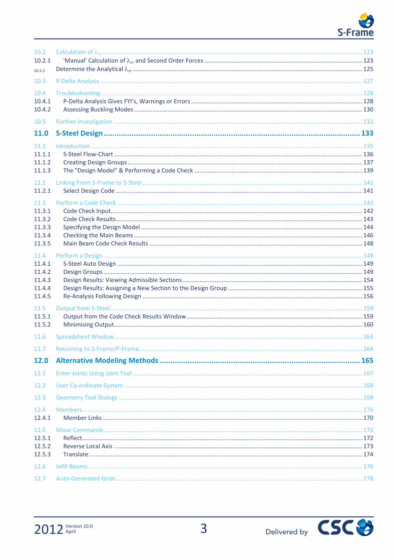
10.2 Calculation of cr ........................................................................................................................................................... 123 10.2.1 'Manual' Calculation of cr and Second Order Forces .............................................................................................. 123
10.2.2 Determine the Analytical cr ......................................................................................................................................... 125
10.3 P-Delta Analysis ............................................................................................................................................................ 127
10.4 Troubleshooting ............................................................................................................................................................ 128 10.4.1 P-Delta Analysis Gives FYI's, Warnings or Errors ...................................................................................................... 128 10.4.2 Assessing Buckling Modes ........................................................................................................................................ 130
10.5 Further Investigation .................................................................................................................................................... 132
11.0 S-Steel Design ....................................................................................................................... 133
11.1 Introduction .................................................................................................................................................................. 135 11.1.1 S-Steel Flow-Chart .................................................................................................................................................... 136 11.1.2 Creating Design Groups ............................................................................................................................................ 137 11.1.3 The "Design Model" & Performing a Code Check .................................................................................................... 139
11.2 Linking From S-Frame to S-Steel ................................................................................................................................... 141 11.2.1 Select Design Code ................................................................................................................................................... 141
11.3 Perform a Code Check .................................................................................................................................................. 142 11.3.1 Code Check Input...................................................................................................................................................... 142 11.3.2 Code Check Results................................................................................................................................................... 143 11.3.3 Specifying the Design Model .................................................................................................................................... 144 11.3.4 Checking the Main Beams ........................................................................................................................................ 146 11.3.5 Main Beam Code Check Results ............................................................................................................................... 148
11.4 Perform a Design .......................................................................................................................................................... 149 11.4.1 S-Steel Auto Design .................................................................................................................................................. 149 11.4.2 Design Groups .......................................................................................................................................................... 149 11.4.3 Design Results: Viewing Admissible Sections ........................................................................................................... 154 11.4.4 Design Results: Assigning a New Section to the Design Group ................................................................................ 155 11.4.5 Re-Analysis Following Design ................................................................................................................................... 156
11.5 Output from S-Steel ...................................................................................................................................................... 159 11.5.1 Output from the Code Check Results Window ......................................................................................................... 159 11.5.2 Minimising Output .................................................................................................................................................... 160
11.6 Spreadsheet Window .................................................................................................................................................... 163
11.7 Returning to S-Frame/P-Frame ..................................................................................................................................... 164
12.0 Alternative Modeling Methods ............................................................................................. 165
12.1 Enter Joints Using Joint Tool ......................................................................................................................................... 167
12.2 User Co-ordinate System .............................................................................................................................................. 168
12.3 Geometry Tool Dialogs ................................................................................................................................................. 169
12.4 Members ....................................................................................................................................................................... 170 12.4.1 Member Links ........................................................................................................................................................... 170
12.5 Move Commands .......................................................................................................................................................... 172 12.5.1 Reflect ....................................................................................................................................................................... 172 12.5.2 Reverse Local Axis .................................................................................................................................................... 173 12.5.3 Translate ................................................................................................................................................................... 174
12.6 Infill Beams.................................................................................................................................................................... 176
12.7 Auto-Generated Grids ................................................................................................................................................... 178


5
Introduction P-Frame & S-Frame Versions
2012 Version 10.0 April
1.0 Introduction

7
Introduction P-Frame & S-Frame Versions
2012 Version 10.0 April
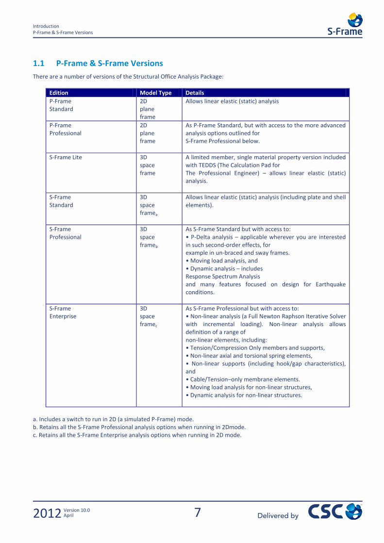
1.1 P-Frame & S-Frame Versions
There are a number of versions of the Structural Office Analysis Package:
Edition Model Type Details
P-Frame Standard
2D plane frame
Allows linear elastic (static) analysis
P-Frame Professional
2D plane frame
As P-Frame Standard, but with access to the more advanced analysis options outlined for S-Frame Professional below.
S-Frame Lite
3D space frame
A limited member, single material property version included with TEDDS (The Calculation Pad for The Professional Engineer) – allows linear elastic (static) analysis.
S-Frame Standard
3D space framea
Allows linear elastic (static) analysis (including plate and shell elements).
S-Frame Professional
3D space frameb
As S-Frame Standard but with access to: • P-Delta analysis – applicable wherever you are interested in such second-order effects, for example in un-braced and sway frames. • Moving load analysis, and • Dynamic analysis – includes Response Spectrum Analysis and many features focused on design for Earthquake conditions.
S-Frame Enterprise
3D space framec
As S-Frame Professional but with access to: • Non-linear analysis (a Full Newton Raphson Iterative Solver with incremental loading). Non-linear analysis allows definition of a range of non-linear elements, including: • Tension/Compression Only members and supports, • Non-linear axial and torsional spring elements, • Non-linear supports (including hook/gap characteristics), and • Cable/Tension–only membrane elements. • Moving load analysis for non-linear structures, • Dynamic analysis for non-linear structures.
a. Includes a switch to run in 2D (a simulated P-Frame) mode. b. Retains all the S-Frame Professional analysis options when running in 2Dmode. c. Retains all the S-Frame Enterprise analysis options when running in 2D mode.
8
Introduction Getting into the Program
2012 Version 10.0 April
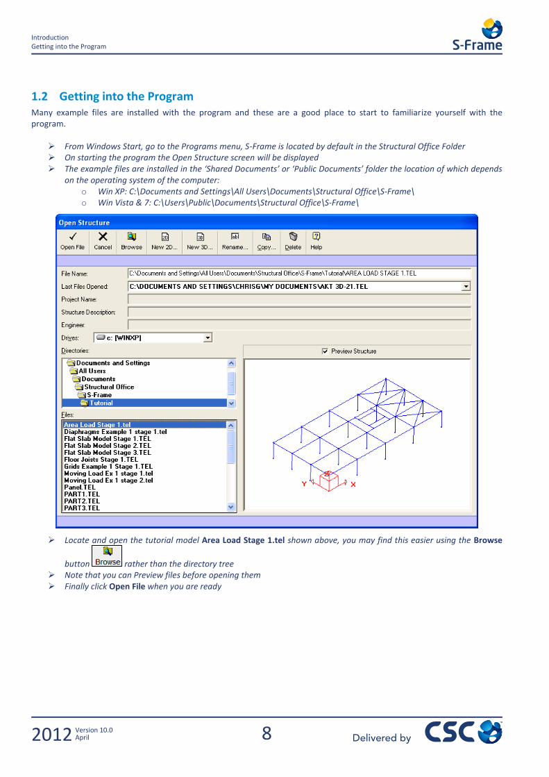
1.2 Getting into the Program Many example files are installed with the program and these are a good place to start to familiarize yourself with the program.
From Windows Start, go to the Programs menu, S-Frame is located by default in the Structural Office Folder On starting the program the Open Structure screen will be displayed The example files are installed in the ‘Shared Documents’ or ‘Public Documents’ folder the location of which depends
on the operating system of the computer: o Win XP: C:\Documents and Settings\All Users\Documents\Structural Office\S-Frame\ o Win Vista & 7: C:\Users\Public\Documents\Structural Office\S-Frame\
Locate and open the tutorial model Area Load Stage 1.tel shown above, you may find this easier using the Browse
button rather than the directory tree Note that you can Preview files before opening them Finally click Open File when you are ready
9
Introduction User Interface
2012 Version 10.0 April
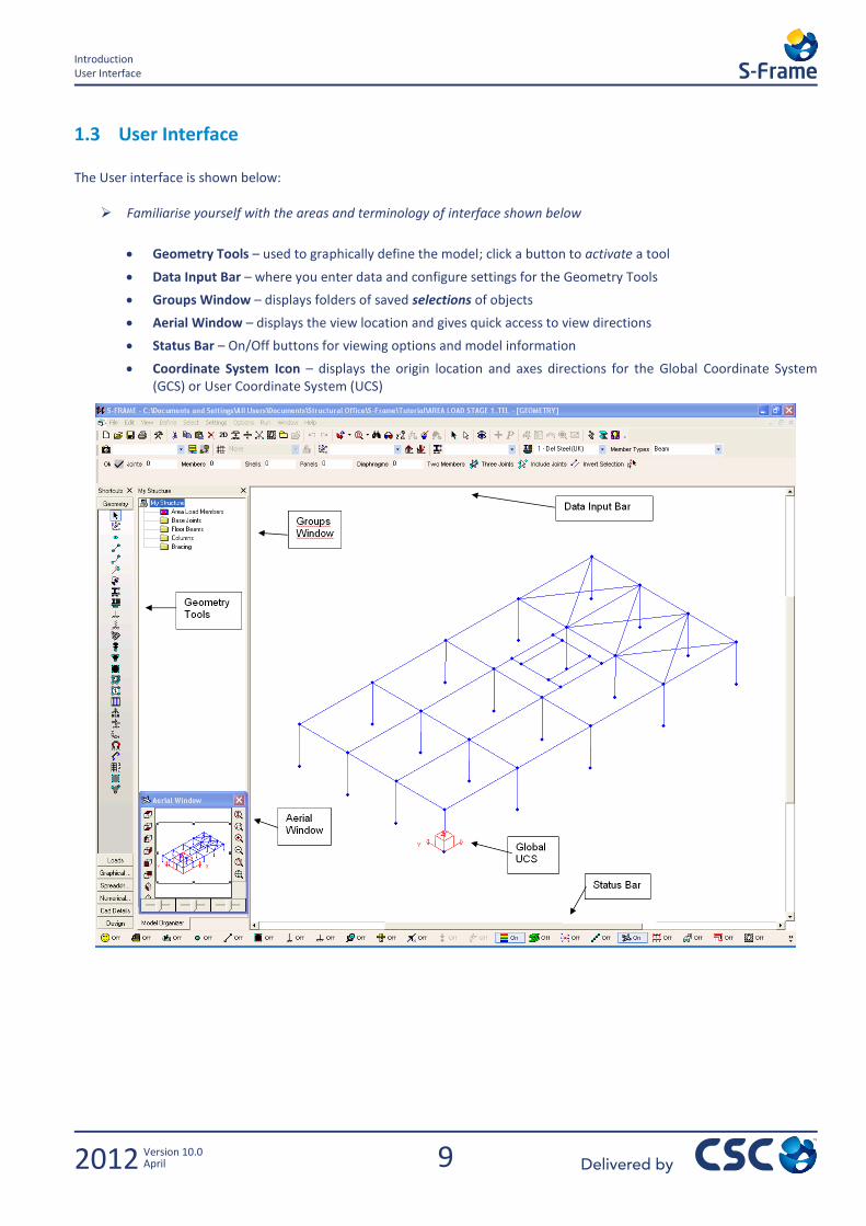
1.3 User Interface The User interface is shown below:
Familiarise yourself with the areas and terminology of interface shown below
Geometry Tools – used to graphically define the model; click a button to activate a tool
Data Input Bar – where you enter data and configure settings for the Geometry Tools
Groups Window – displays folders of saved selections of objects
Aerial Window – displays the view location and gives quick access to view directions
Status Bar – On/Off buttons for viewing options and model information
Coordinate System Icon – displays the origin location and axes directions for the Global Coordinate System (GCS) or User Coordinate System (UCS)
10
Introduction 2D and 3D Model Types
2012 Version 10.0 April
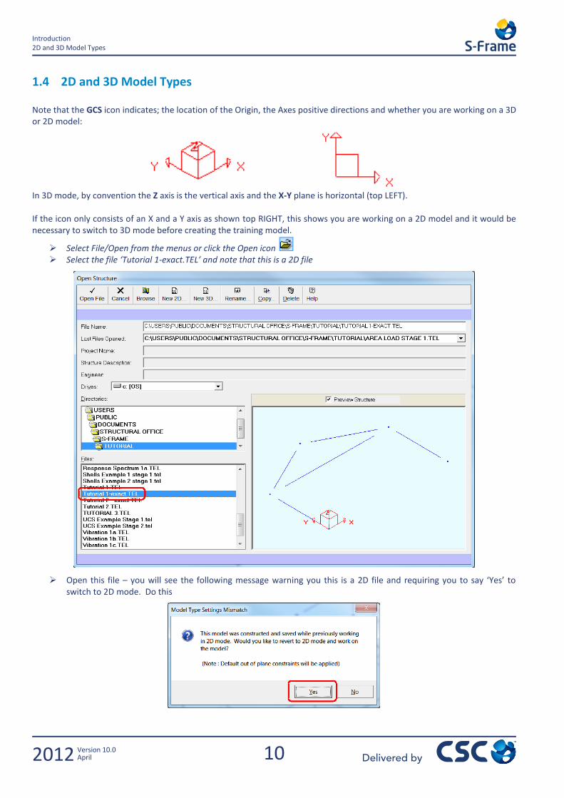
1.4 2D and 3D Model Types Note that the GCS icon indicates; the location of the Origin, the Axes positive directions and whether you are working on a 3D or 2D model:
In 3D mode, by convention the Z axis is the vertical axis and the X-Y plane is horizontal (top LEFT). If the icon only consists of an X and a Y axis as shown top RIGHT, this shows you are working on a 2D model and it would be necessary to switch to 3D mode before creating the training model.
Select File/Open from the menus or click the Open icon Select the file ‘Tutorial 1-exact.TEL’ and note that this is a 2D file
Open this file – you will see the following message warning you this is a 2D file and requiring you to say ‘Yes’ to switch to 2D mode. Do this
11
Introduction 2D and 3D Model Types
2012 Version 10.0 April
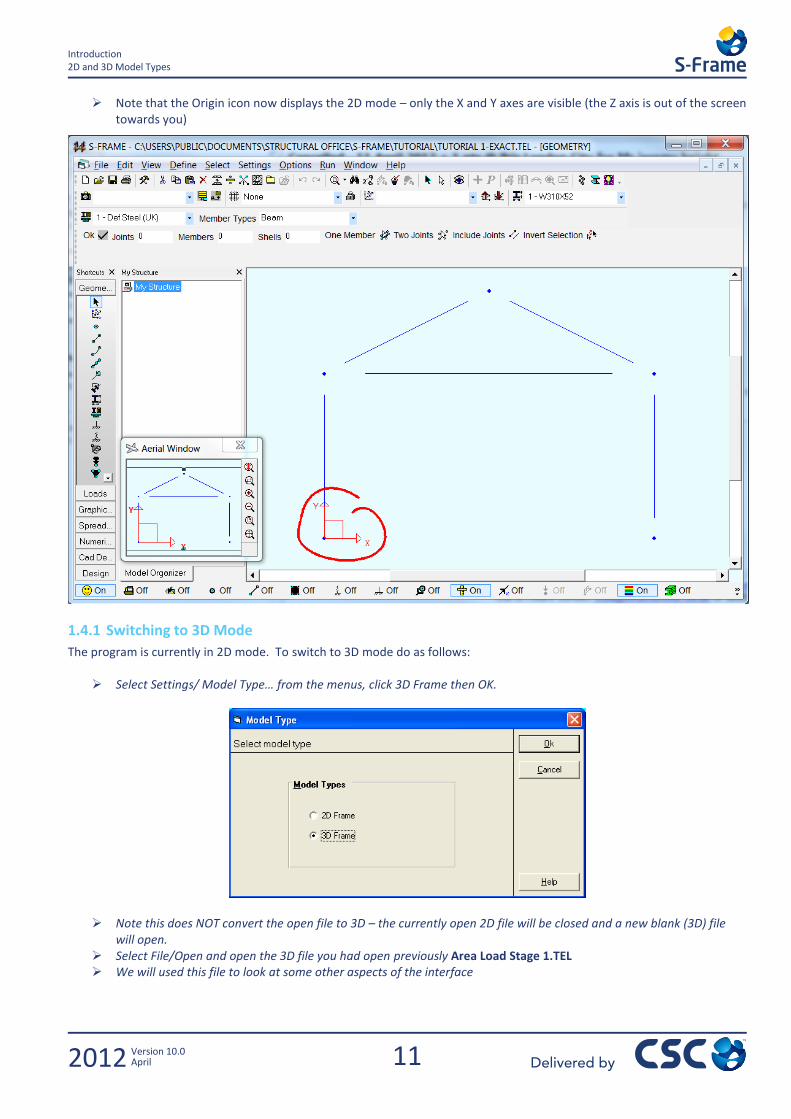
Note that the Origin icon now displays the 2D mode – only the X and Y axes are visible (the Z axis is out of the screen towards you)
1.4.1 Switching to 3D Mode
The program is currently in 2D mode. To switch to 3D mode do as follows:
Select Settings/ Model Type… from the menus, click 3D Frame then OK.
Note this does NOT convert the open file to 3D – the currently open 2D file will be closed and a new blank (3D) file will open.
Select File/Open and open the 3D file you had open previously Area Load Stage 1.TEL We will used this file to look at some other aspects of the interface
12
Introduction The Status Bar
2012 Version 10.0 April
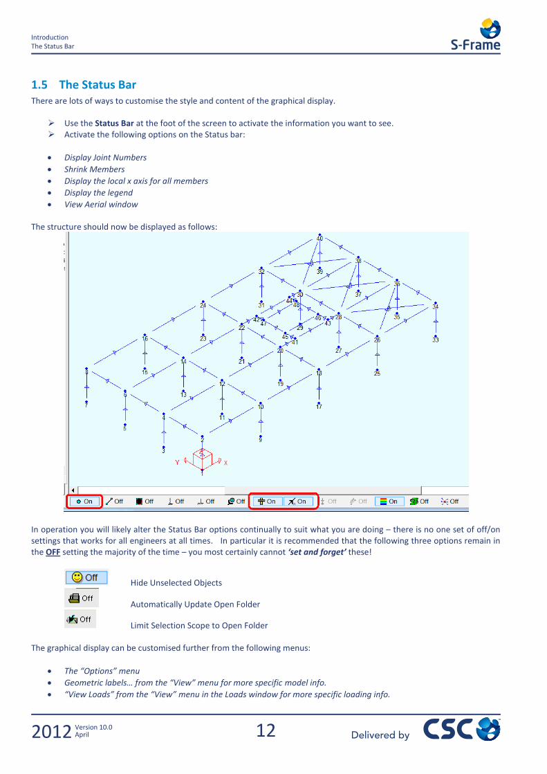
1.5 The Status Bar There are lots of ways to customise the style and content of the graphical display.
Use the Status Bar at the foot of the screen to activate the information you want to see. Activate the following options on the Status bar:
Display Joint Numbers
Shrink Members
Display the local x axis for all members
Display the legend
View Aerial window The structure should now be displayed as follows:
In operation you will likely alter the Status Bar options continually to suit what you are doing – there is no one set of off/on settings that works for all engineers at all times. In particular it is recommended that the following three options remain in the OFF setting the majority of the time – you most certainly cannot ‘set and forget’ these!
Hide Unselected Objects
Automatically Update Open Folder
Limit Selection Scope to Open Folder The graphical display can be customised further from the following menus:
The “Options” menu
Geometric labels… from the “View” menu for more specific model info.
“View Loads” from the “View” menu in the Loads window for more specific loading info.
13
Introduction The Selection Tool
2012 Version 10.0 April
1.6 The Selection Tool It is essential that you are comfortable with the different ways to select and unselect elements. You can only edit elements when they are selected - unselected objects are frozen and cannot be edited. By selecting several elements at the same time, you can quickly perform an edit on all of them at once. The selected elements could be:
Copied or Deleted
The Element Type, Section, Material etc. changed
End releases added/changed
Supports added/changed So before building the model it is worth mastering the various selection techniques.
1.6.1 Selection using the Menu
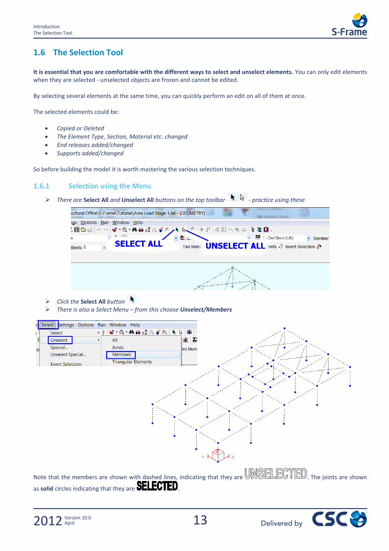
There are Select All and Unselect All buttons on the top toolbar - practice using these
Click the Select All button There is also a Select Menu – from this choose Unselect/Members
Note that the members are shown with dashed lines, indicating that they are . The joints are shown
as solid circles indicating that they are .
14
Introduction The Selection Tool
2012 Version 10.0 April
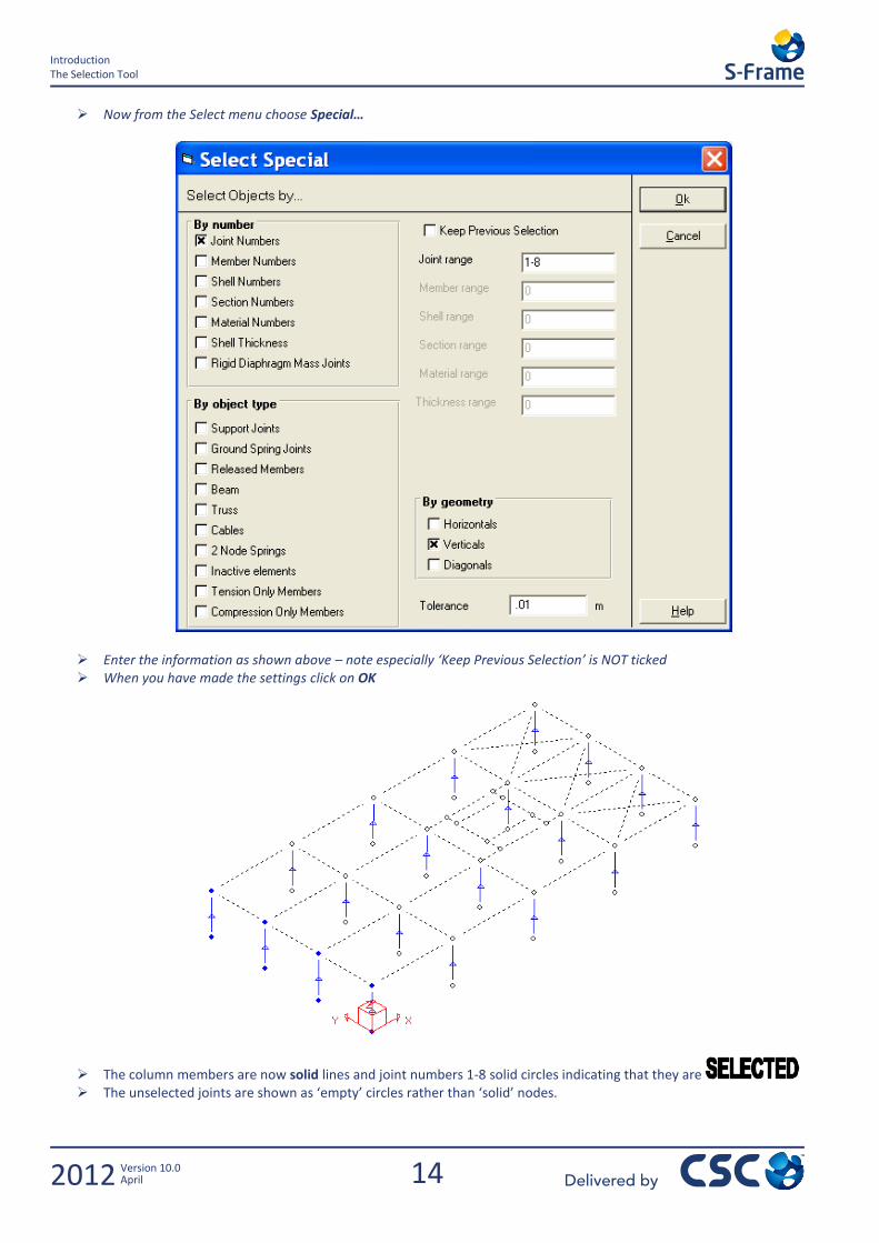
Now from the Select menu choose Special…
Enter the information as shown above – note especially ‘Keep Previous Selection’ is NOT ticked When you have made the settings click on OK
The column members are now solid lines and joint numbers 1-8 solid circles indicating that they are The unselected joints are shown as ‘empty’ circles rather than ‘solid’ nodes.
15
Introduction The Selection Tool
2012 Version 10.0 April
1.6.2 Selection via Group Folders
What are Group Folders? They are simply Saved Selections of Objects – nothing more and nothing less. Group folders are similar in concept to layers in AutoCAD – while you could use AutoCAD without using layers this would not be very efficient. The same applies to S-FRAME and Groups.
Objects are; Joints, Members, Shells, and Panels. Note that things like Material and Section are not objects, these are Properties of objects and are not saved in groups as such. A group simply defines which objects are selected or not; if an object is selected its properties will be visible and can be edited.
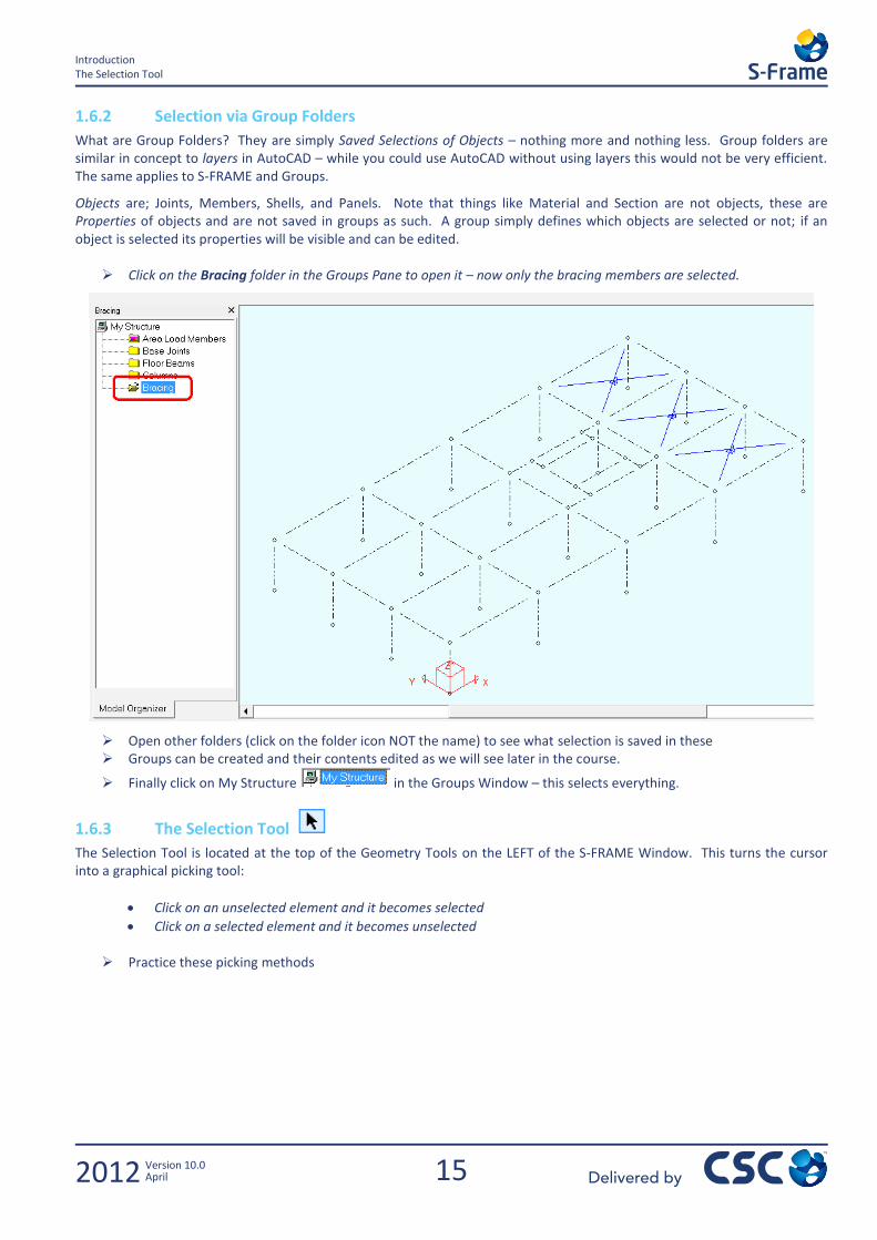
Click on the Bracing folder in the Groups Pane to open it – now only the bracing members are selected.
Open other folders (click on the folder icon NOT the name) to see what selection is saved in these Groups can be created and their contents edited as we will see later in the course.
Finally click on My Structure in the Groups Window – this selects everything.
1.6.3 The Selection Tool
The Selection Tool is located at the top of the Geometry Tools on the LEFT of the S-FRAME Window. This turns the cursor into a graphical picking tool:
Click on an unselected element and it becomes selected
Click on a selected element and it becomes unselected
Practice these picking methods
16
Introduction The Selection Tool
2012 Version 10.0 April
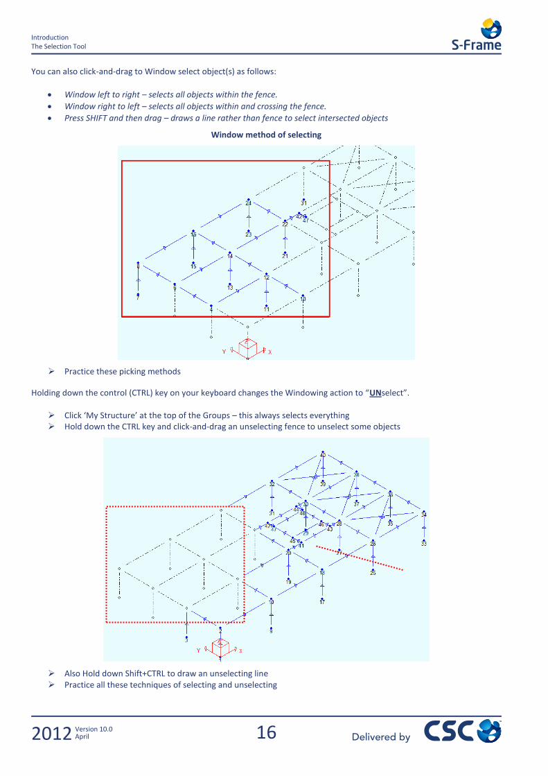
You can also click-and-drag to Window select object(s) as follows:
Window left to right – selects all objects within the fence.
Window right to left – selects all objects within and crossing the fence.
Press SHIFT and then drag – draws a line rather than fence to select intersected objects
Window method of selecting
Practice these picking methods
Holding down the control (CTRL) key on your keyboard changes the Windowing action to “UNselect”.
Click ‘My Structure’ at the top of the Groups – this always selects everything Hold down the CTRL key and click-and-drag an unselecting fence to unselect some objects
Also Hold down Shift+CTRL to draw an unselecting line Practice all these techniques of selecting and unselecting
17
Introduction Setting Preferences
2012 Version 10.0 April
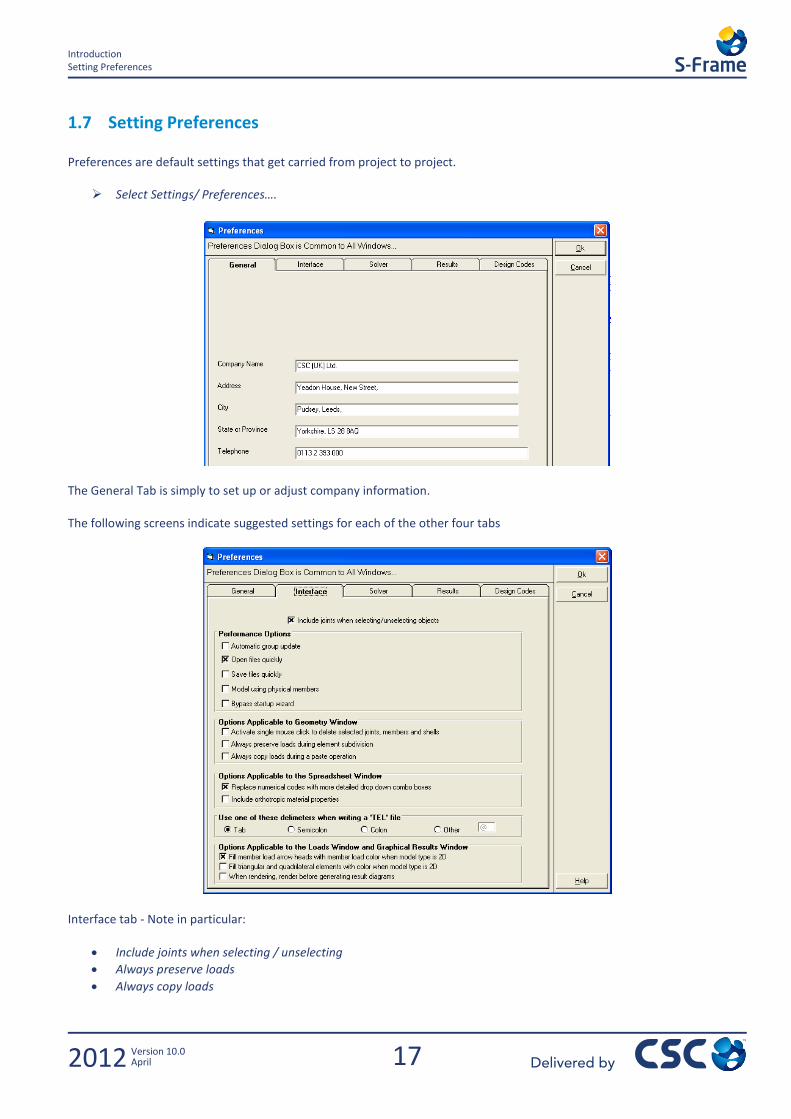
1.7 Setting Preferences Preferences are default settings that get carried from project to project.
Select Settings/ Preferences….
The General Tab is simply to set up or adjust company information. The following screens indicate suggested settings for each of the other four tabs
Interface tab - Note in particular:
Include joints when selecting / unselecting
Always preserve loads
Always copy loads
18
Introduction Setting Preferences
2012 Version 10.0 April
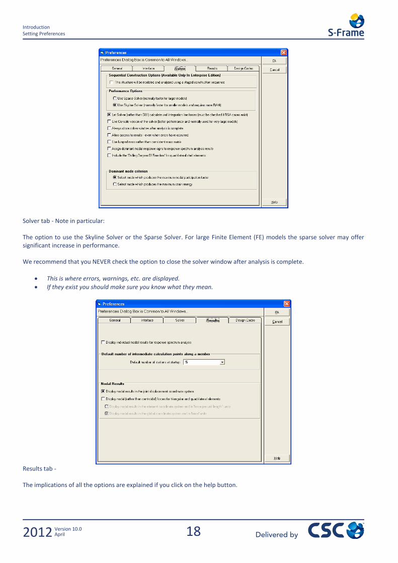
Solver tab - Note in particular: The option to use the Skyline Solver or the Sparse Solver. For large Finite Element (FE) models the sparse solver may offer significant increase in performance. We recommend that you NEVER check the option to close the solver window after analysis is complete.
This is where errors, warnings, etc. are displayed.
If they exist you should make sure you know what they mean.
Results tab - The implications of all the options are explained if you click on the help button.
19
Introduction Setting Preferences
2012 Version 10.0 April
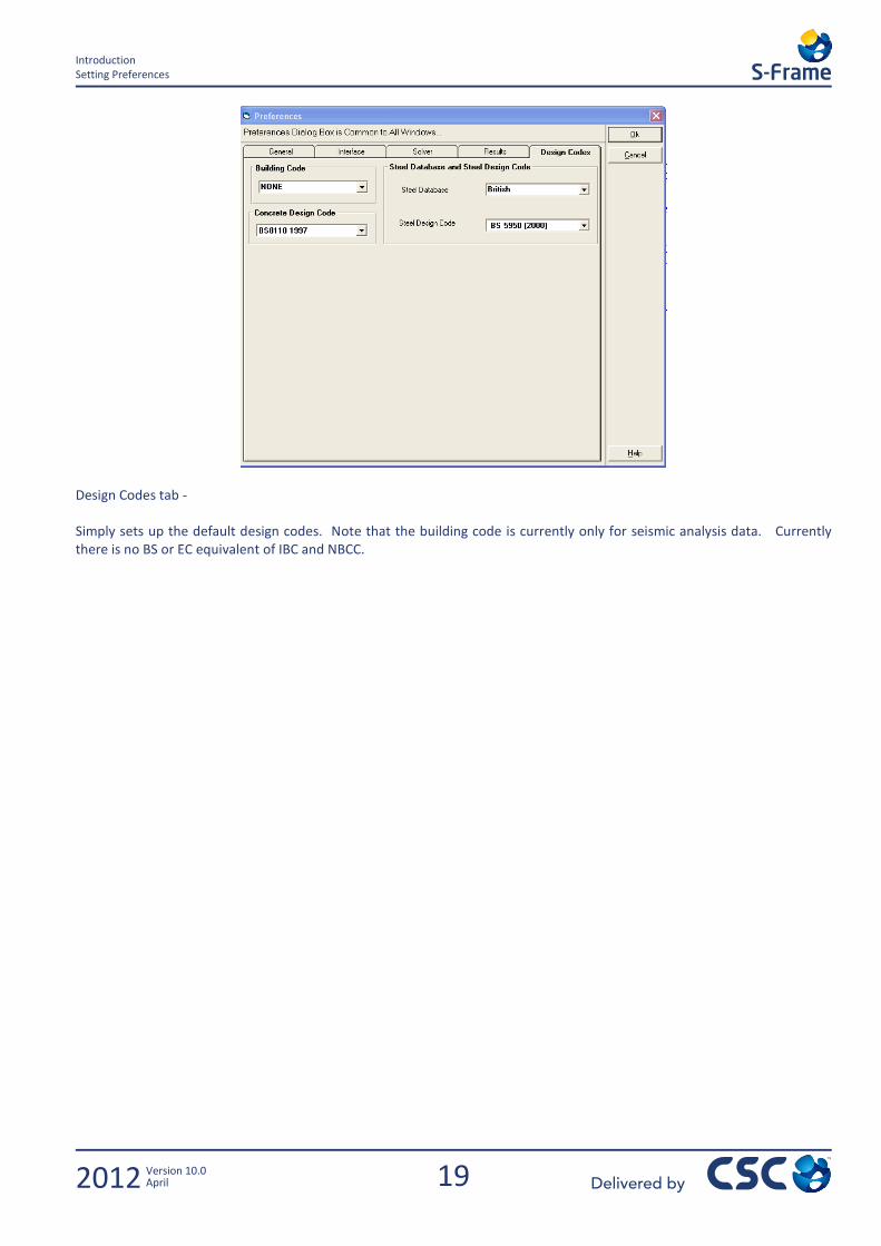
Design Codes tab - Simply sets up the default design codes. Note that the building code is currently only for seismic analysis data. Currently there is no BS or EC equivalent of IBC and NBCC.


21
Geometry Window
2012 Version 10.0 April
2.0 Geometry Window


23
Geometry Window Starting a New Project
2012 Version 10.0 April
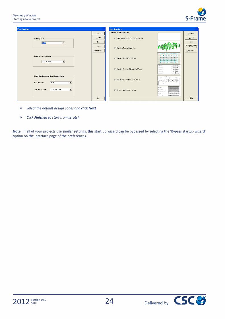
2.1 Starting a New Project
Make sure you are in 3D mode, then Select File/New
Fill in some details and click Next
Select the Input Units and click Next
Select the Results Units and click Next Select the Modelling Options and click Next
24
Geometry Window Starting a New Project
2012 Version 10.0 April
Select the default design codes and click Next Click Finished to start from scratch
Note: If all of your projects use similar settings, this start up wizard can be bypassed by selecting the ‘Bypass startup wizard’ option on the Interface page of the preferences.
25
Geometry Window Using the Grid
2012 Version 10.0 April
2.2 Using the Grid
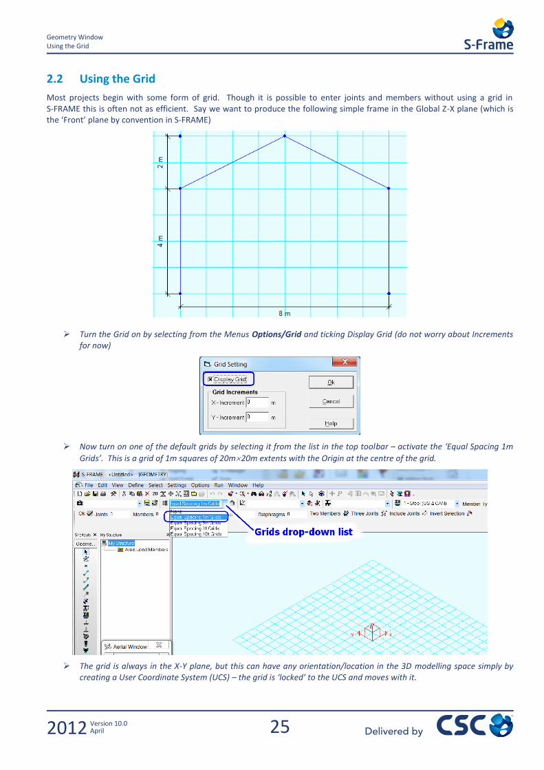
Most projects begin with some form of grid. Though it is possible to enter joints and members without using a grid in S-FRAME this is often not as efficient. Say we want to produce the following simple frame in the Global Z-X plane (which is the ‘Front’ plane by convention in S-FRAME)
Turn the Grid on by selecting from the Menus Options/Grid and ticking Display Grid (do not worry about Increments for now)
Now turn on one of the default grids by selecting it from the list in the top toolbar – activate the ‘Equal Spacing 1m
Grids’. This is a grid of 1m squares of 20m20m extents with the Origin at the centre of the grid.
The grid is always in the X-Y plane, but this can have any orientation/location in the 3D modelling space simply by creating a User Coordinate System (UCS) – the grid is ‘locked’ to the UCS and moves with it.
26
Geometry Window Using the Grid
2012 Version 10.0 April
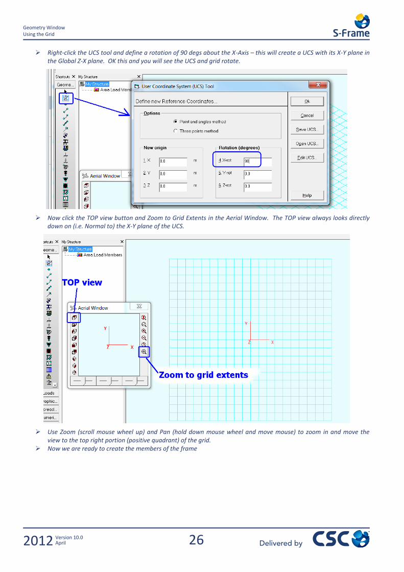
Right-click the UCS tool and define a rotation of 90 degs about the X-Axis – this will create a UCS with its X-Y plane in the Global Z-X plane. OK this and you will see the UCS and grid rotate.
Now click the TOP view button and Zoom to Grid Extents in the Aerial Window. The TOP view always looks directly down on (i.e. Normal to) the X-Y plane of the UCS.
Use Zoom (scroll mouse wheel up) and Pan (hold down mouse wheel and move mouse) to zoom in and move the view to the top right portion (positive quadrant) of the grid.
Now we are ready to create the members of the frame
27
Geometry Window Using the Grid
2012 Version 10.0 April
2.2.1 Create Members on the Grid
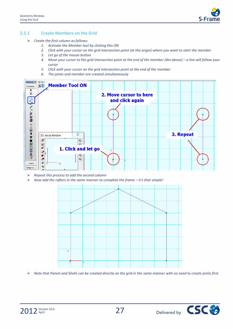
Create the first column as follows: 1. Activate the Member tool by clicking this ON 2. Click with your cursor on the grid intersection point (at the origin) where you want to start the member 3. Let go of the mouse button 4. Move your cursor to the grid intersection point at the end of the member (4m above) – a line will follow your
cursor 5. Click with your cursor on the grid intersection point at the end of the member 6. The joints and member are created simultaneously
Repeat this process to add the second column Now add the rafters in the same manner to complete the frame – it’s that simple!
Note that Panels and Shells can be created directly on the grid in the same manner with no need to create joints first.
28
Geometry Window Using the Grid
2012 Version 10.0 April
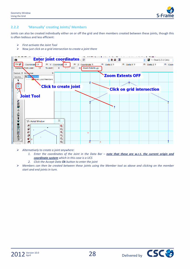
2.2.2 ‘Manually’ creating Joints/ Members
Joints can also be created individually either on or off the grid and then members created between these joints, though this is often tedious and less efficient:
First activate the Joint Tool Now just click on a grid intersection to create a joint there
Alternatively to create a joint anywhere: 1. Enter the coordinates of the Joint in the Data Bar – note that these are w.r.t. the current origin and
coordinate system which in this case is a UCS 2. Click the Accept Data Ok button to enter the joint
Members can then be created between these joints using the Member tool as above and clicking on the member start and end joints in turn.
29
Geometry Window Using the Grid
2012 Version 10.0 April
2.2.3 More Grid Functions
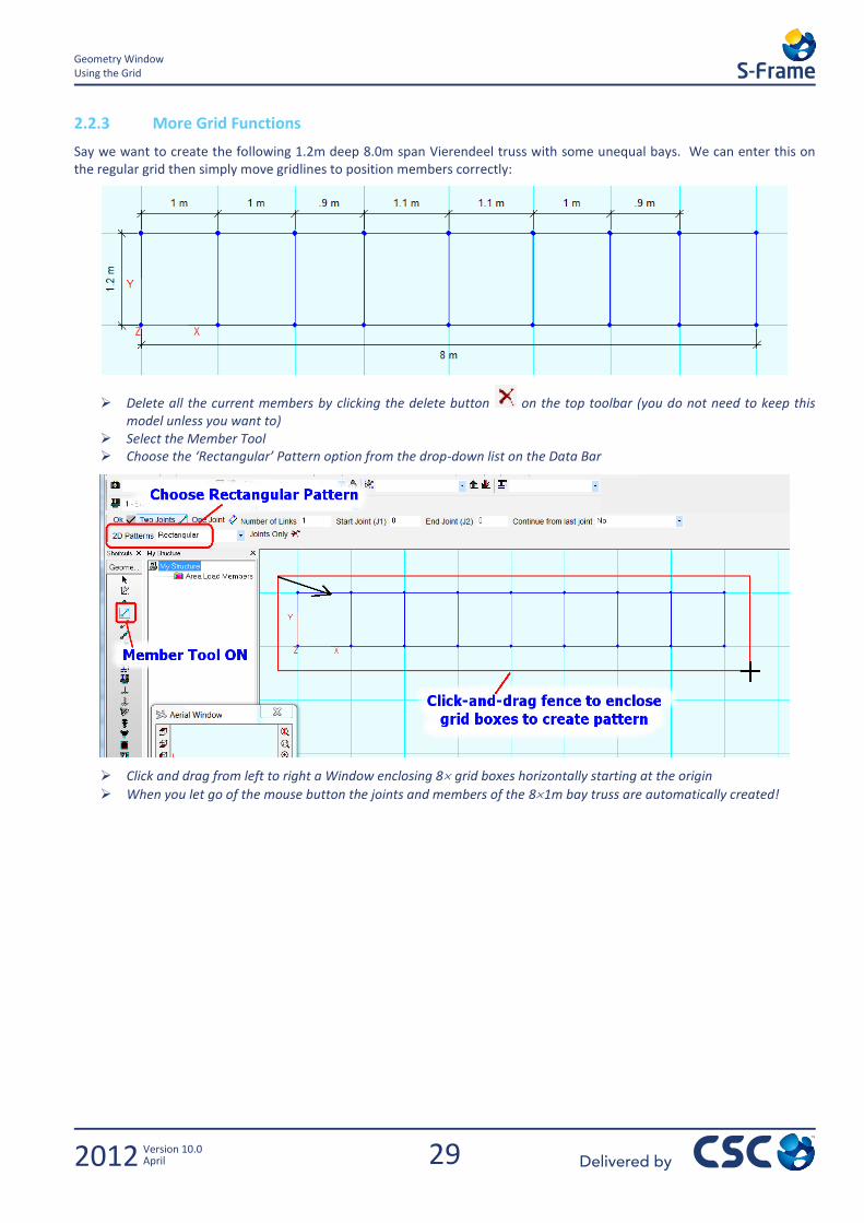
Say we want to create the following 1.2m deep 8.0m span Vierendeel truss with some unequal bays. We can enter this on the regular grid then simply move gridlines to position members correctly:
Delete all the current members by clicking the delete button on the top toolbar (you do not need to keep this model unless you want to)
Select the Member Tool Choose the ‘Rectangular’ Pattern option from the drop-down list on the Data Bar
Click and drag from left to right a Window enclosing 8 grid boxes horizontally starting at the origin
When you let go of the mouse button the joints and members of the 81m bay truss are automatically created!
30
Geometry Window Using the Grid
2012 Version 10.0 April
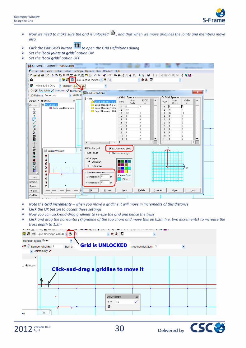
Now we need to make sure the grid is unlocked , and that when we move gridlines the joints and members move also
Click the Edit Grids button to open the Grid Definitions dialog Set the ‘Lock joints to grids’ option ON Set the ‘Lock grids’ option OFF
Note the Grid increments – when you move a gridline it will move in increments of this distance Click the OK button to accept these settings Now you can click-and-drag gridlines to re-size the grid and hence the truss Click and drag the horizontal (Y) gridline of the top chord and move this up 0.2m (i.e. two increments) to increase the
truss depth to 1.2m
31
Geometry Window Using the Grid
2012 Version 10.0 April
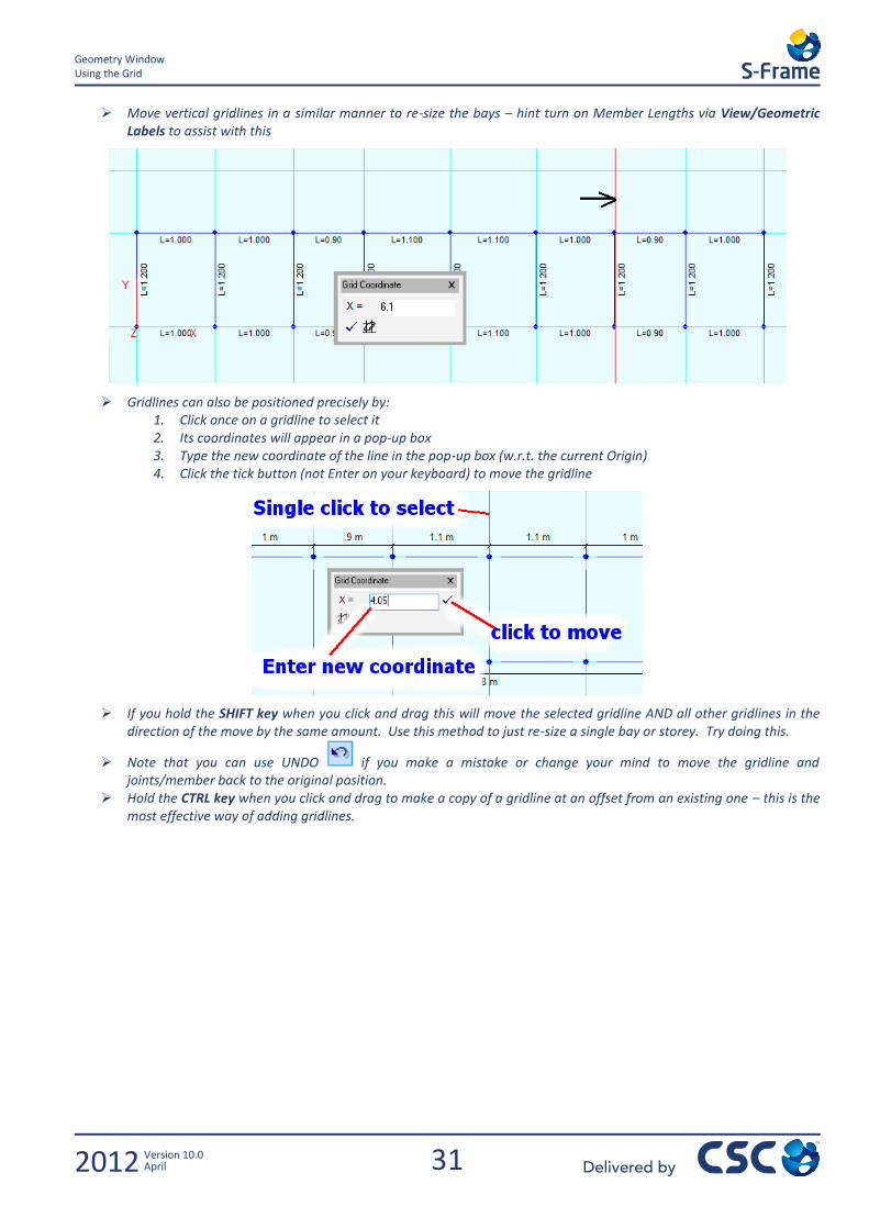
Move vertical gridlines in a similar manner to re-size the bays – hint turn on Member Lengths via View/Geometric Labels to assist with this
Gridlines can also be positioned precisely by: 1. Click once on a gridline to select it 2. Its coordinates will appear in a pop-up box 3. Type the new coordinate of the line in the pop-up box (w.r.t. the current Origin) 4. Click the tick button (not Enter on your keyboard) to move the gridline
If you hold the SHIFT key when you click and drag this will move the selected gridline AND all other gridlines in the direction of the move by the same amount. Use this method to just re-size a single bay or storey. Try doing this.
Note that you can use UNDO if you make a mistake or change your mind to move the gridline and joints/member back to the original position.
Hold the CTRL key when you click and drag to make a copy of a gridline at an offset from an existing one – this is the most effective way of adding gridlines.
32
Geometry Window Using the Grid
2012 Version 10.0 April
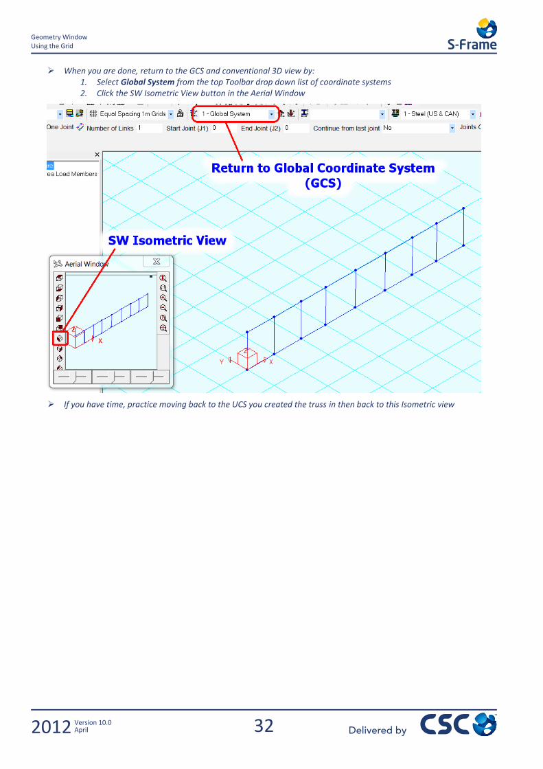
When you are done, return to the GCS and conventional 3D view by: 1. Select Global System from the top Toolbar drop down list of coordinate systems 2. Click the SW Isometric View button in the Aerial Window
If you have time, practice moving back to the UCS you created the truss in then back to this Isometric view
33
Geometry Window Saving UCS’s and Views
2012 Version 10.0 April
2.3 Saving UCS’s and Views
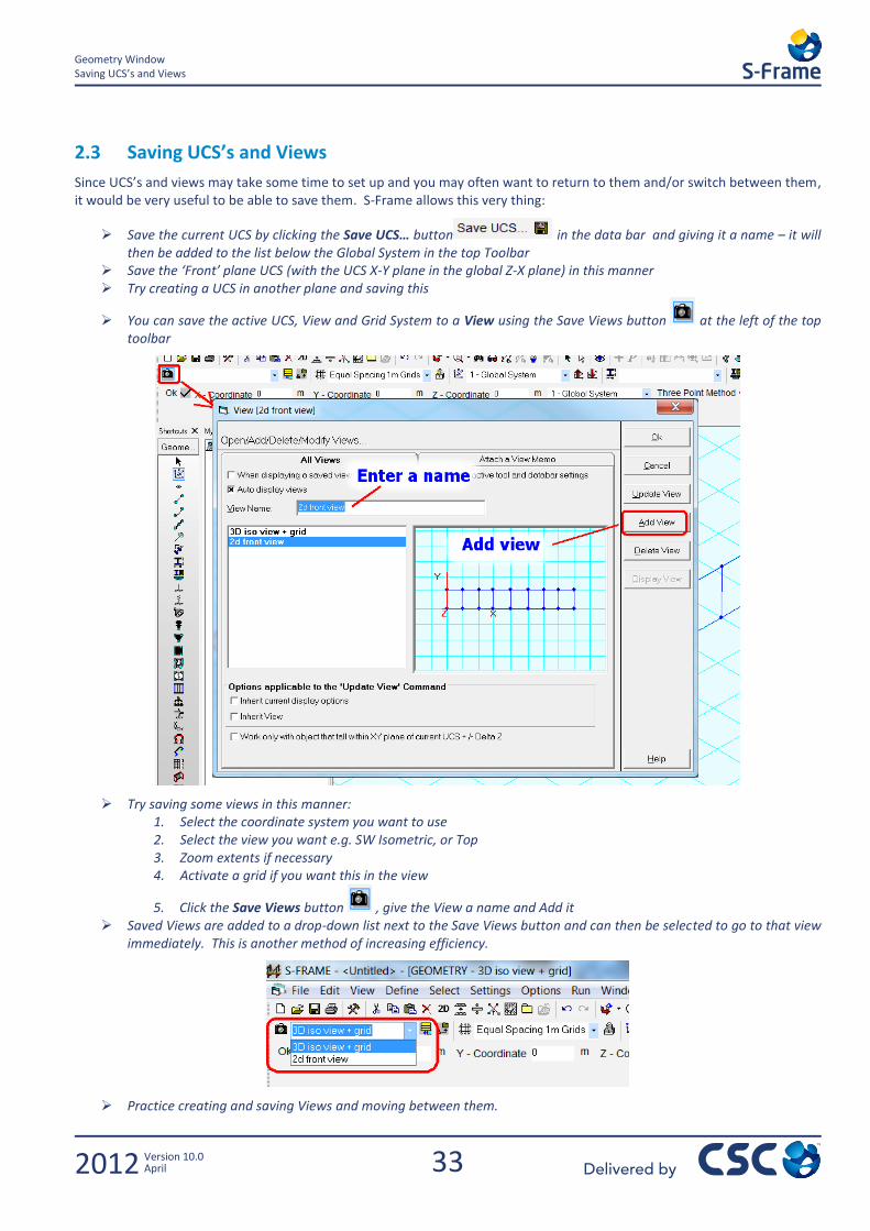
Since UCS’s and views may take some time to set up and you may often want to return to them and/or switch between them, it would be very useful to be able to save them. S-Frame allows this very thing:
Save the current UCS by clicking the Save UCS… button in the data bar and giving it a name – it will then be added to the list below the Global System in the top Toolbar
Save the ‘Front’ plane UCS (with the UCS X-Y plane in the global Z-X plane) in this manner Try creating a UCS in another plane and saving this
You can save the active UCS, View and Grid System to a View using the Save Views button at the left of the top toolbar
Try saving some views in this manner: 1. Select the coordinate system you want to use 2. Select the view you want e.g. SW Isometric, or Top 3. Zoom extents if necessary 4. Activate a grid if you want this in the view
5. Click the Save Views button , give the View a name and Add it Saved Views are added to a drop-down list next to the Save Views button and can then be selected to go to that view
immediately. This is another method of increasing efficiency.
Practice creating and saving Views and moving between them.
34
Geometry Window Physical Members
2012 Version 10.0 April
2.4 Physical Members
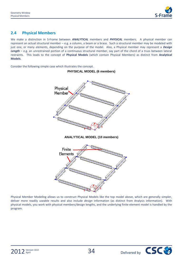
We make a distinction in S-Frame between ANALYTICAL members and PHYSICAL members. A physical member can represent an actual structural member – e.g. a column, a beam or a brace. Such a structural member may be modeled with just one, or many elements, depending on the purpose of the model. Also, a Physical member may represent a Design Length – e.g. an unrestrained portion of a continuous structural member, say part of the chord of a truss between lateral restraints. This leads to the concept of Physical Models (which contain Physical Members) as distinct from Analytical Models. Consider the following simple case which illustrates the concept.
PHYSICAL MODEL (6 members)
ANALYTICAL MODEL (10 members)
Physical Member Modeling allows us to construct Physical Models like the top model above, which are generally simpler, deliver more readily useable results and also include design information (as distinct from Analysis information). With physical models, you work with physical members/design lengths, and the underlying finite element model is handled by the program.
35
Geometry Window Physical Members
2012 Version 10.0 April
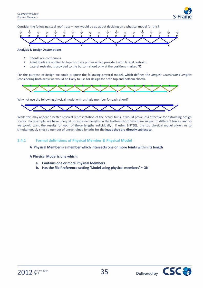
Consider the following steel roof truss – how would be go about deciding on a physical model for this?
Analysis & Design Assumptions
Chords are continuous. Point loads are applied to top chord via purlins which provide it with lateral restraint. Lateral restraint is provided to the bottom chord only at the positions marked 'X'
For the purpose of design we could propose the following physical model, which defines the longest unrestrained lengths (considering both axes) we would be likely to use for design for both top and bottom chords.
Why not use the following physical model with a single member for each chord?
While this may appear a better physical representation of the actual truss, it would prove less effective for extracting design forces. For example, we have unequal unrestrained lengths in the bottom chord which are subject to different forces, and so we would want the results for each of these lengths individually. If using S-STEEL, the top physical model allows us to simultaneously check a number of unrestrained lengths for the loads they are directly subject to.
2.4.1 Formal definitions of Physical Member & Physical Model
A Physical Member is a member which intersects one or more Joints within its length
A Physical Model is one which:
a. Contains one or more Physical Members b. Has the file Preference setting ‘Model using physical members’ = ON

36
Geometry Window Physical Members
2012 Version 10.0 April

37
Training Project Model Physical Members
2012 Version 10.0 April
3.0 Training Project Model

38
Training Project Model Project Brief
2012 Version 10.0 April
39
Training Project Model Project Brief
2012 Version 10.0 April
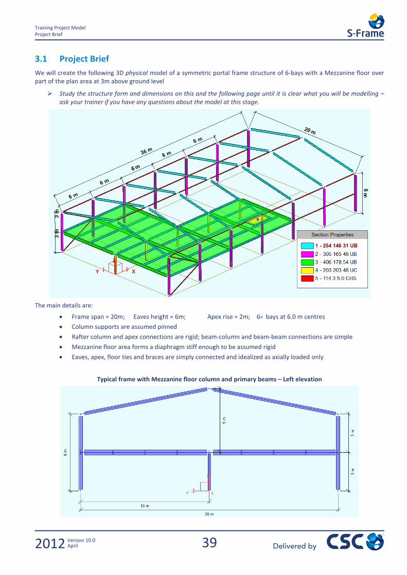
3.1 Project Brief
We will create the following 3D physical model of a symmetric portal frame structure of 6-bays with a Mezzanine floor over part of the plan area at 3m above ground level
Study the structure form and dimensions on this and the following page until it is clear what you will be modelling – ask your trainer if you have any questions about the model at this stage.
The main details are:
Frame span = 20m; Eaves height = 6m; Apex rise = 2m; 6 bays at 6.0 m centres
Column supports are assumed pinned
Rafter column and apex connections are rigid; beam-column and beam-beam connections are simple
Mezzanine floor area forms a diaphragm stiff enough to be assumed rigid
Eaves, apex, floor ties and braces are simply connected and idealized as axially loaded only
Typical frame with Mezzanine floor column and primary beams – Left elevation
40
Training Project Model Project Brief
2012 Version 10.0 April
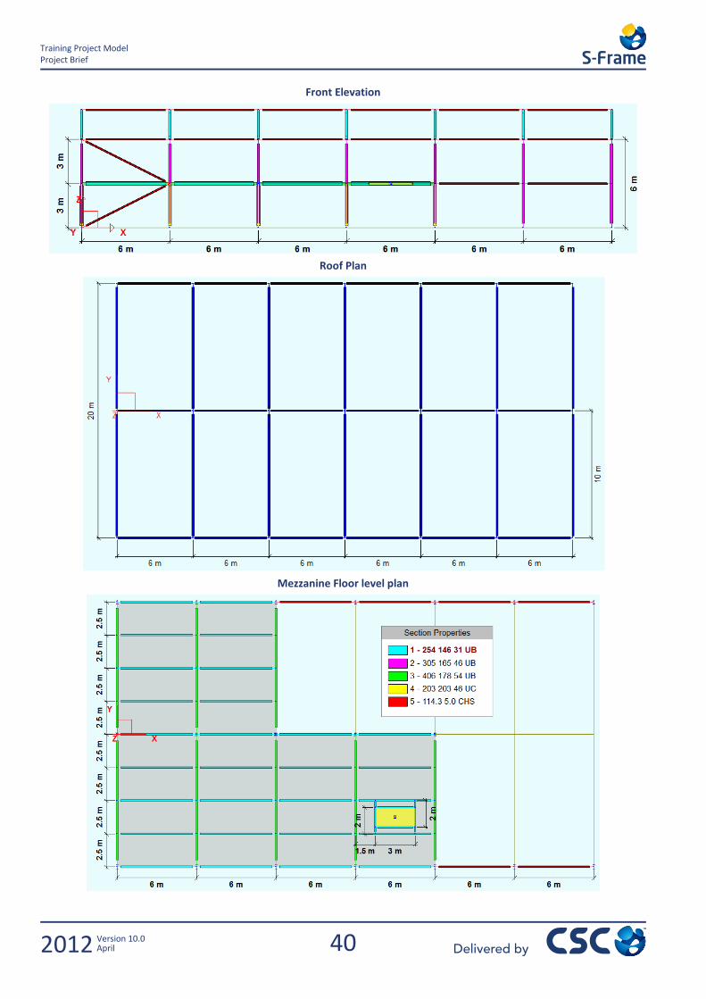
Front Elevation
Roof Plan
Mezzanine Floor level plan
41
Training Project Model Start a New Project
2012 Version 10.0 April
3.2 Start a New Project We will construct the model in the following sequence:
1. Create the typical Frame shown on pg 39 above in the Y-Z plane
2. Apply to this frame appropriate; releases, supports, member-orientation, sections, material
3. Create 6 copies of the frame at 6m centres in the X-direction
4. Create the Mezzanine floor joists
5. Add the ties and bracing
6. Add floor trimming steel and slab (area load surface and diaphragm)
7. Apply loads and load combinations
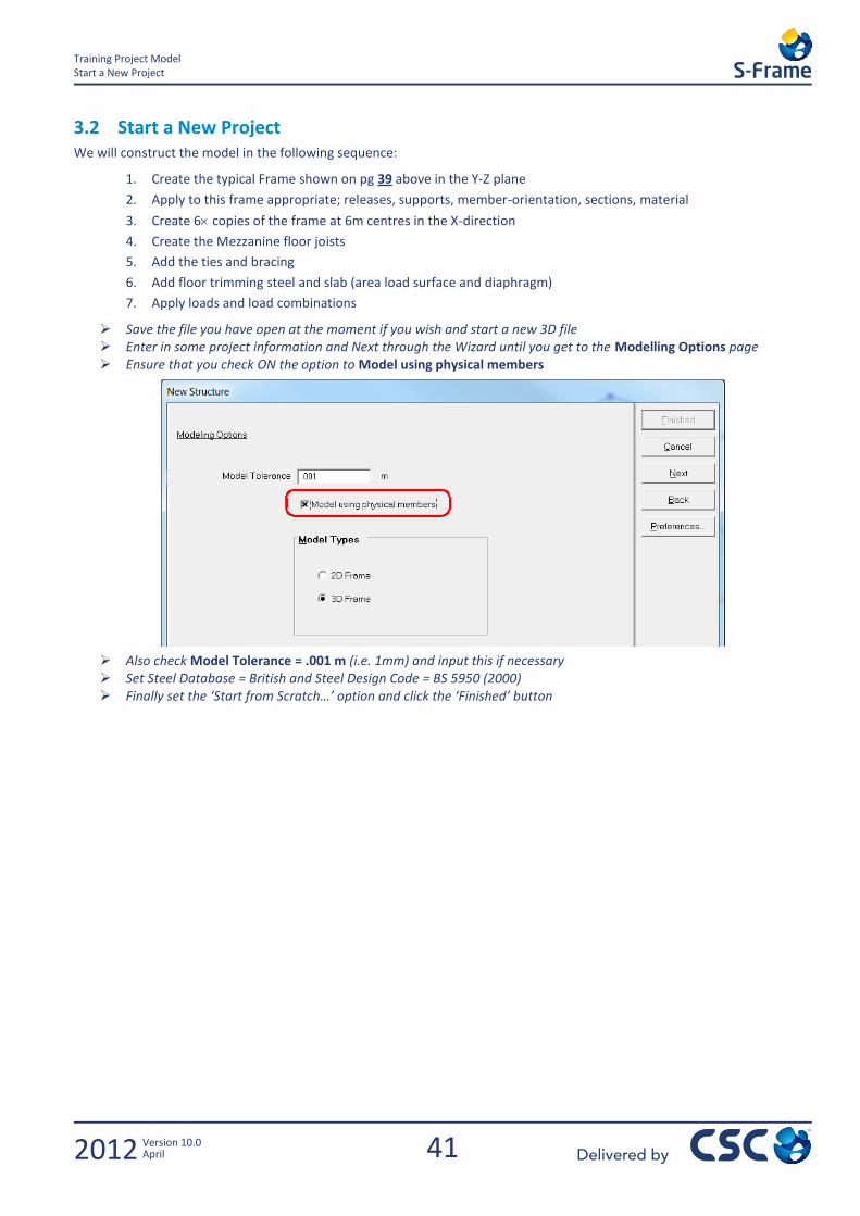
Save the file you have open at the moment if you wish and start a new 3D file Enter in some project information and Next through the Wizard until you get to the Modelling Options page Ensure that you check ON the option to Model using physical members
Also check Model Tolerance = .001 m (i.e. 1mm) and input this if necessary Set Steel Database = British and Steel Design Code = BS 5950 (2000) Finally set the ‘Start from Scratch…’ option and click the ‘Finished’ button
42
Training Project Model Start a New Project
2012 Version 10.0 April
3.2.1 Create Model Grid
We could create the typical frame using the method above of setting up a UCS to place the 1m Grid in the Y-Z vertical plane, however we will demonstrate another method:
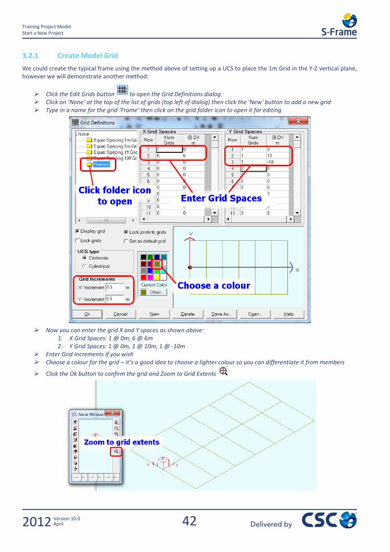
Click the Edit Grids button to open the Grid Definitions dialog Click on ‘None’ at the top of the list of grids (top left of dialog) then click the ‘New’ button to add a new grid Type in a name for the grid ‘Frame’ then click on the grid folder icon to open it for editing
Now you can enter the grid X and Y spaces as shown above: 1. X Grid Spaces: 1 @ 0m, 6 @ 6m 2. Y Grid Spaces: 1 @ 0m, 1 @ 10m, 1 @ -10m
Enter Grid Increments if you wish Choose a colour for the grid – it’s a good idea to choose a lighter colour so you can differentiate it from members
Click the Ok button to confirm the grid and Zoom to Grid Extents

43
Training Project Model Start a New Project
2012 Version 10.0 April
Now it is very simple to use the ‘One Joint’ member creation method to create the two 6m stanchions for the frame Activate the Member Tool and then in the Databar
1. Select the One Joint method 2. Set the +Z direction (up) 3. Enter Member Length = 6m 4. Single click on the (0,10) and (0,-10) grid intersections in turn to create the stanchion members
Next we wish to create the middle mezzanine column and a joint for the apex; we can do this easily by adding a 3m vertical member and a further 5m member on top of this. It is quite legitimate to use members as construction lines to locate joints and delete them afterwards.
Change Member Length = 3m and click on the grid intersection at the origin Change Member Length = 5m (3m to eaves + 2m rise) and click on the joint at the top of the member you just created
Now we have all the required columns and the apex joint
44
Training Project Model Start a New Project
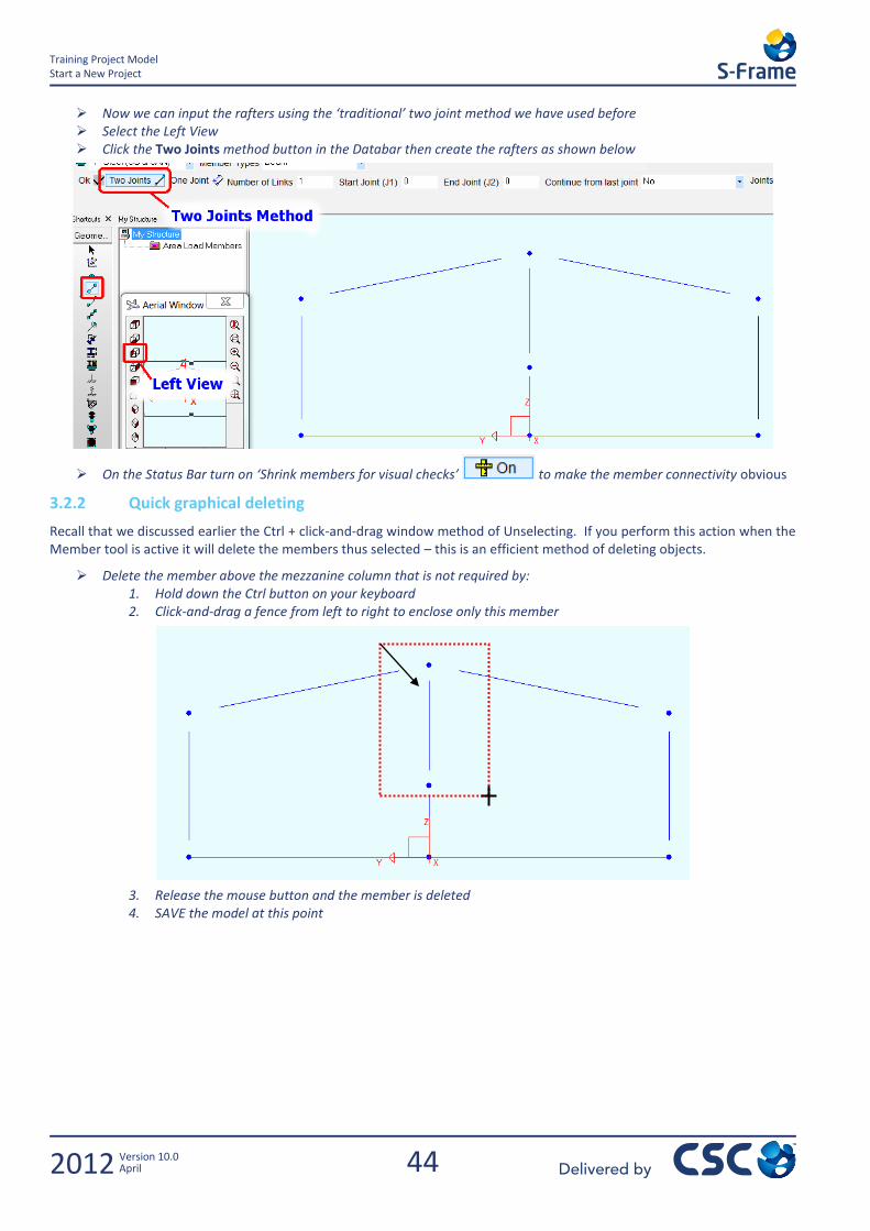
2012 Version 10.0 April
Now we can input the rafters using the ‘traditional’ two joint method we have used before Select the Left View Click the Two Joints method button in the Databar then create the rafters as shown below
On the Status Bar turn on ‘Shrink members for visual checks’ to make the member connectivity obvious
3.2.2 Quick graphical deleting
Recall that we discussed earlier the Ctrl + click-and-drag window method of Unselecting. If you perform this action when the Member tool is active it will delete the members thus selected – this is an efficient method of deleting objects.
Delete the member above the mezzanine column that is not required by: 1. Hold down the Ctrl button on your keyboard 2. Click-and-drag a fence from left to right to enclose only this member
3. Release the mouse button and the member is deleted 4. SAVE the model at this point
45
Training Project Model Start a New Project
2012 Version 10.0 April
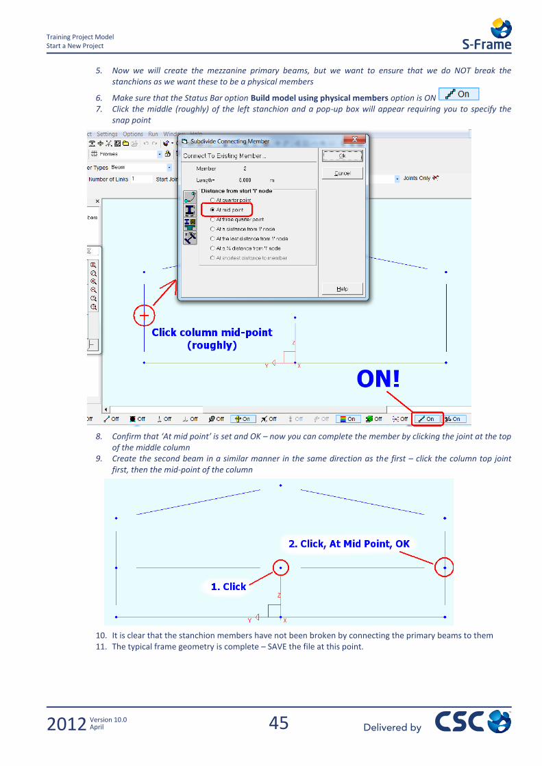
5. Now we will create the mezzanine primary beams, but we want to ensure that we do NOT break the stanchions as we want these to be a physical members
6. Make sure that the Status Bar option Build model using physical members option is ON 7. Click the middle (roughly) of the left stanchion and a pop-up box will appear requiring you to specify the
snap point
8. Confirm that ‘At mid point’ is set and OK – now you can complete the member by clicking the joint at the top of the middle column
9. Create the second beam in a similar manner in the same direction as the first – click the column top joint first, then the mid-point of the column
10. It is clear that the stanchion members have not been broken by connecting the primary beams to them 11. The typical frame geometry is complete – SAVE the file at this point.
46
Training Project Model Releases
2012 Version 10.0 April
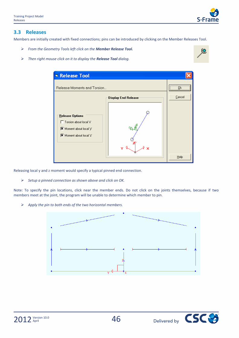
3.3 Releases Members are initially created with fixed connections; pins can be introduced by clicking on the Member Releases Tool.
From the Geometry Tools left click on the Member Release Tool.
Then right mouse click on it to display the Release Tool dialog.
Releasing local y and z moment would specify a typical pinned end connection.
Setup a pinned connection as shown above and click on OK. Note: To specify the pin locations, click near the member ends. Do not click on the joints themselves, because if two members meet at the joint, the program will be unable to determine which member to pin.
Apply the pin to both ends of the two horizontal members.
47
Training Project Model Supports
2012 Version 10.0 April
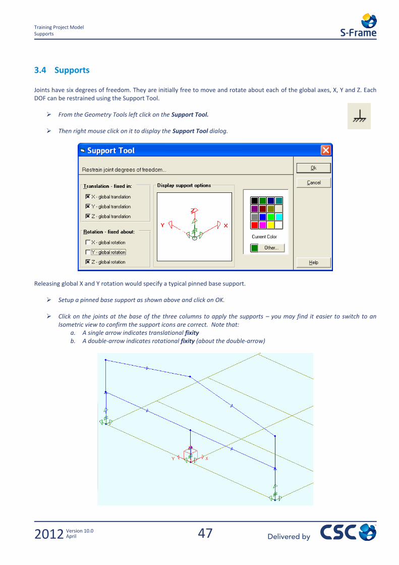
3.4 Supports Joints have six degrees of freedom. They are initially free to move and rotate about each of the global axes, X, Y and Z. Each DOF can be restrained using the Support Tool.
From the Geometry Tools left click on the Support Tool.
Then right mouse click on it to display the Support Tool dialog.
Releasing global X and Y rotation would specify a typical pinned base support.
Setup a pinned base support as shown above and click on OK. Click on the joints at the base of the three columns to apply the supports – you may find it easier to switch to an
Isometric view to confirm the support icons are correct. Note that: a. A single arrow indicates translational fixity b. A double-arrow indicates rotational fixity (about the double-arrow)
48
Training Project Model Member Axis Orientation
2012 Version 10.0 April
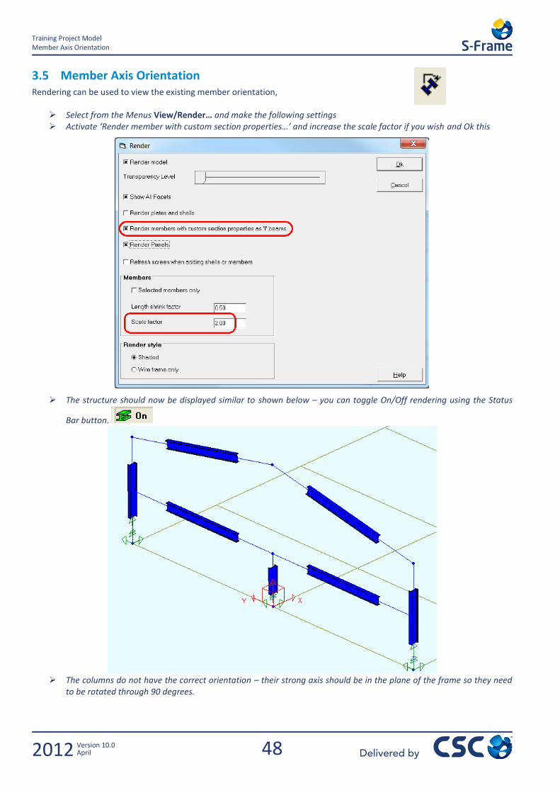
3.5 Member Axis Orientation Rendering can be used to view the existing member orientation,
Select from the Menus View/Render… and make the following settings Activate ‘Render member with custom section properties…’ and increase the scale factor if you wish and Ok this
The structure should now be displayed similar to shown below – you can toggle On/Off rendering using the Status
Bar button.
The columns do not have the correct orientation – their strong axis should be in the plane of the frame so they need
to be rotated through 90 degrees.
49
Training Project Model Member Axis Orientation
2012 Version 10.0 April
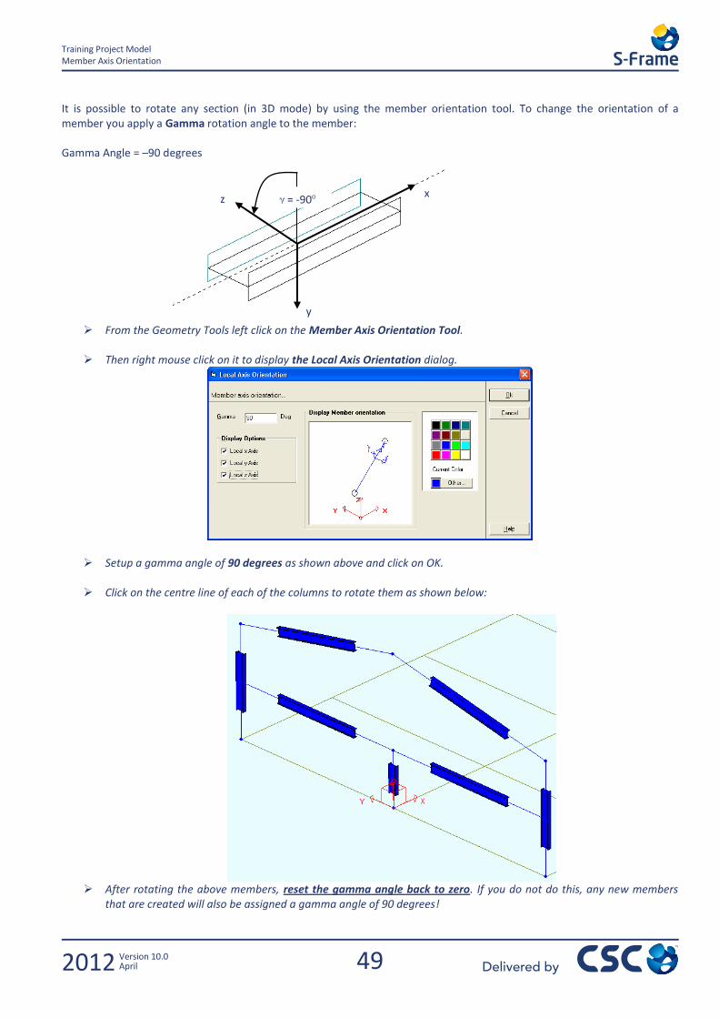
It is possible to rotate any section (in 3D mode) by using the member orientation tool. To change the orientation of a member you apply a Gamma rotation angle to the member: Gamma Angle = –90 degrees
From the Geometry Tools left click on the Member Axis Orientation Tool.
Then right mouse click on it to display the Local Axis Orientation dialog.
Setup a gamma angle of 90 degrees as shown above and click on OK.
Click on the centre line of each of the columns to rotate them as shown below:
After rotating the above members, reset the gamma angle back to zero. If you do not do this, any new members
that are created will also be assigned a gamma angle of 90 degrees!
y
x z = -90
50
Training Project Model Folder Grouping
2012 Version 10.0 April
3.6 Folder Grouping Now that a frame has been created, members can be grouped together to facilitate handling the model.
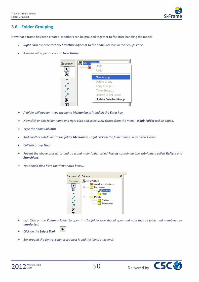
Right Click over the text My Structure adjacent to the Computer icon in the Groups Pane.
A menu will appear - click on New Group
A folder will appear - type the name Mezzanine in it and hit the Enter key.
Now click on this folder name and right click and select New Group from the menu - a Sub-Folder will be added.
Type the name Columns
Add another sub-folder to the folder Mezzanine - right click on the folder name, select New Group
Call this group Floor
Repeat the above process to add a second main folder called Portals containing two sub-folders called Rafters and Stanchions.
You should then have the view shown below.
Left Click on the Columns folder to open it - the folder icon should open and note that all joints and members are unselected.
Click on the Select Tool
Box around the central column to select it and the joints at its ends.
51
Training Project Model Folder Grouping
2012 Version 10.0 April
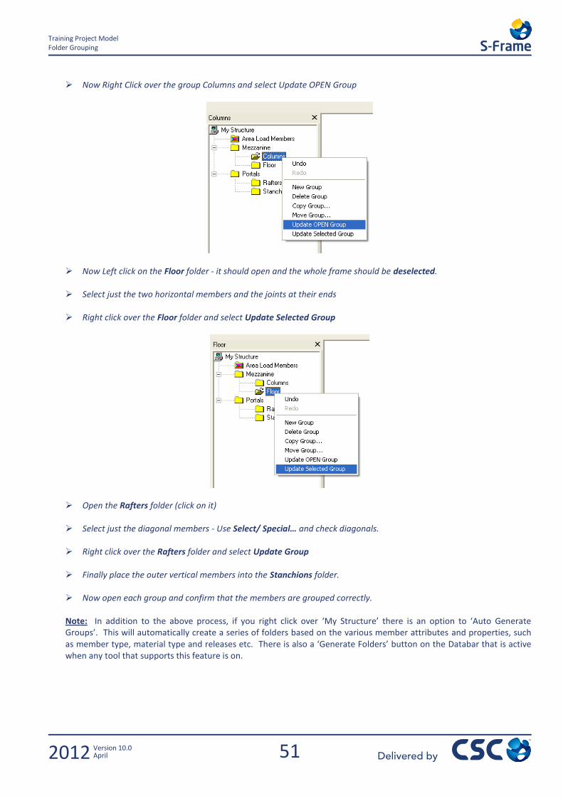
Now Right Click over the group Columns and select Update OPEN Group
Now Left click on the Floor folder - it should open and the whole frame should be deselected.
Select just the two horizontal members and the joints at their ends
Right click over the Floor folder and select Update Selected Group
Open the Rafters folder (click on it)
Select just the diagonal members - Use Select/ Special… and check diagonals.
Right click over the Rafters folder and select Update Group
Finally place the outer vertical members into the Stanchions folder.
Now open each group and confirm that the members are grouped correctly.
Note: In addition to the above process, if you right click over ‘My Structure’ there is an option to ‘Auto Generate Groups’. This will automatically create a series of folders based on the various member attributes and properties, such as member type, material type and releases etc. There is also a ‘Generate Folders’ button on the Databar that is active when any tool that supports this feature is on.
52
Training Project Model Sections
2012 Version 10.0 April
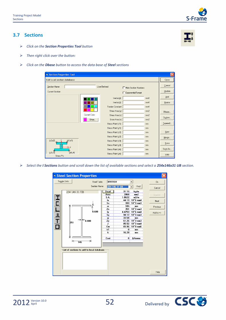
3.7 Sections
Click on the Section Properties Tool button
Then right click over the button:
Click on the Dbase button to access the data base of Steel sections
Select the I Sections button and scroll down the list of available sections and select a 254x146x31 UB section.
53
Training Project Model Sections
2012 Version 10.0 April
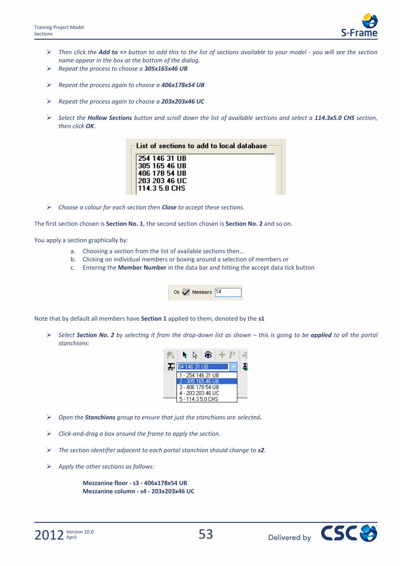
Then click the Add to => button to add this to the list of sections available to your model - you will see the section name appear in the box at the bottom of the dialog.
Repeat the process to choose a 305x165x46 UB
Repeat the process again to choose a 406x178x54 UB
Repeat the process again to choose a 203x203x46 UC
Select the Hollow Sections button and scroll down the list of available sections and select a 114.3x5.0 CHS section, then click OK.
Choose a colour for each section then Close to accept these sections. The first section chosen is Section No. 1, the second section chosen is Section No. 2 and so on. You apply a section graphically by:
a. Choosing a section from the list of available sections then… b. Clicking on individual members or boxing around a selection of members or c. Entering the Member Number in the data bar and hitting the accept data tick button
Note that by default all members have Section 1 applied to them, denoted by the s1
Select Section No. 2 by selecting it from the drop-down list as shown – this is going to be applied to all the portal stanchions:
Open the Stanchions group to ensure that just the stanchions are selected.
Click-and-drag a box around the frame to apply the section.
The section identifier adjacent to each portal stanchion should change to s2.
Apply the other sections as follows:
Mezzanine floor - s3 - 406x178x54 UB Mezzanine column - s4 - 203x203x46 UC
54
Training Project Model Sections
2012 Version 10.0 April
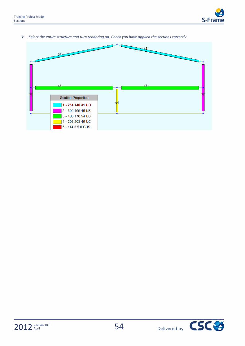
Select the entire structure and turn rendering on. Check you have applied the sections correctly
55
Training Project Model Materials
2012 Version 10.0 April
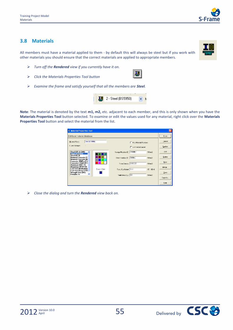
3.8 Materials All members must have a material applied to them - by default this will always be steel but if you work with other materials you should ensure that the correct materials are applied to appropriate members.
Turn off the Rendered view if you currently have it on.
Click the Materials Properties Tool button Examine the frame and satisfy yourself that all the members are Steel.
Note: The material is denoted by the text m1, m2, etc. adjacent to each member, and this is only shown when you have the Materials Properties Tool button selected. To examine or edit the values used for any material, right click over the Materials Properties Tool button and select the material from the list.
Close the dialog and turn the Rendered view back on.
56
Training Project Model Generate
2012 Version 10.0 April
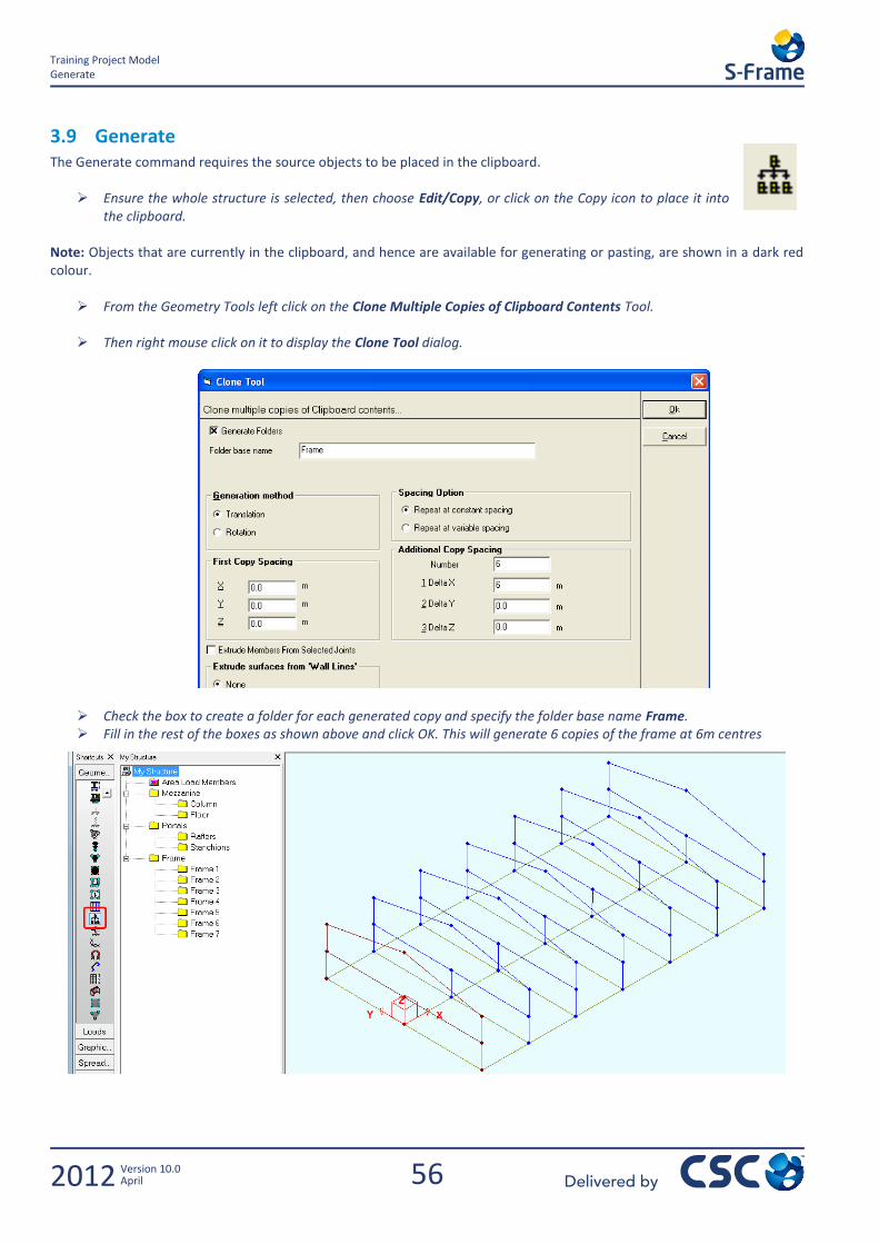
3.9 Generate The Generate command requires the source objects to be placed in the clipboard.
Ensure the whole structure is selected, then choose Edit/Copy, or click on the Copy icon to place it into the clipboard.
Note: Objects that are currently in the clipboard, and hence are available for generating or pasting, are shown in a dark red colour.
From the Geometry Tools left click on the Clone Multiple Copies of Clipboard Contents Tool.
Then right mouse click on it to display the Clone Tool dialog.
Check the box to create a folder for each generated copy and specify the folder base name Frame. Fill in the rest of the boxes as shown above and click OK. This will generate 6 copies of the frame at 6m centres
57
Training Project Model Delete
2012 Version 10.0 April
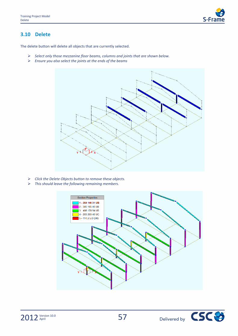
3.10 Delete The delete button will delete all objects that are currently selected.
Select only those mezzanine floor beams, columns and joints that are shown below. Ensure you also select the joints at the ends of the beams
Click the Delete Objects button to remove these objects. This should leave the following remaining members.
58
Training Project Model 2D Plane toggle
2012 Version 10.0 April
3.11 2D Plane toggle
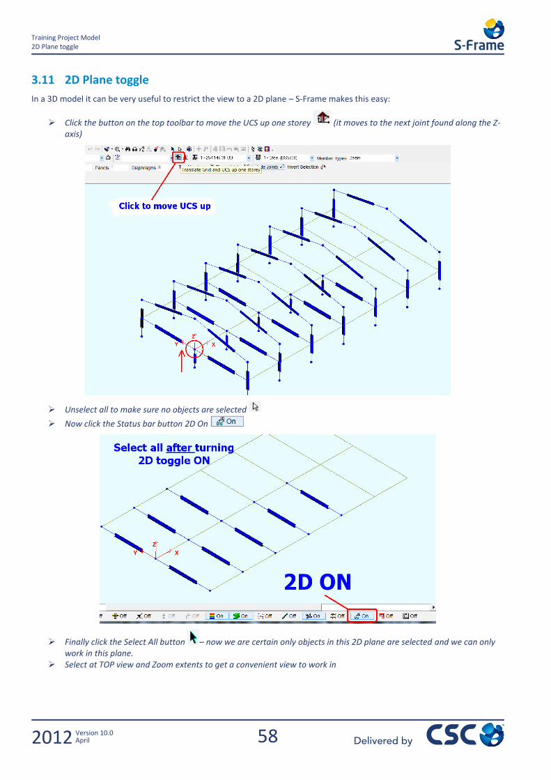
In a 3D model it can be very useful to restrict the view to a 2D plane – S-Frame makes this easy:
Click the button on the top toolbar to move the UCS up one storey (it moves to the next joint found along the Z-axis)
Unselect all to make sure no objects are selected
Now click the Status bar button 2D On
Finally click the Select All button – now we are certain only objects in this 2D plane are selected and we can only work in this plane.
Select at TOP view and Zoom extents to get a convenient view to work in
59
Training Project Model Infill Beams
2012 Version 10.0 April
3.12 Infill Beams
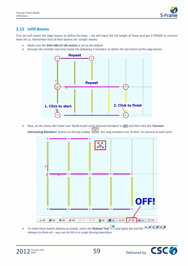
First we will create the edge beams to define the bays – we will input the full length of these and get S-FRAME to connect them for us. Remember that all floor beams are ‘simple’ beams.
Make sure the 25414631 UB section is set as the default Activate the member tool and create the following 3 members to define the full extent of the edge beams
Now, on the Status Bar make sure ‘Build model using physical members’ is OFF and then click the ‘Connect
Intersecting Members’ button on the top toolbar - the long members are ‘broken’ to connect to each joint
To make these beams behave as simple, select the Release Tool and apply My and Mz releases to them all – you can do this in a single fencing operation.
60
Training Project Model Automatic Joist creation
2012 Version 10.0 April
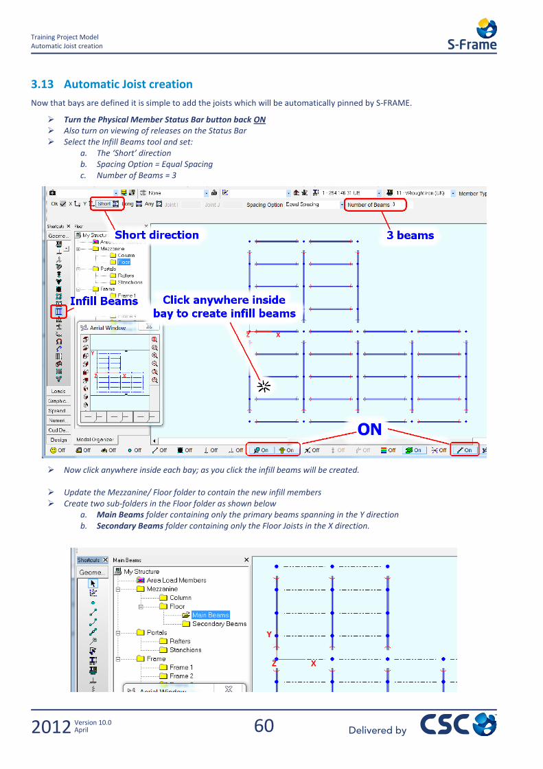
3.13 Automatic Joist creation
Now that bays are defined it is simple to add the joists which will be automatically pinned by S-FRAME.
Turn the Physical Member Status Bar button back ON Also turn on viewing of releases on the Status Bar Select the Infill Beams tool and set:
a. The ‘Short’ direction b. Spacing Option = Equal Spacing c. Number of Beams = 3
Now click anywhere inside each bay; as you click the infill beams will be created.
Update the Mezzanine/ Floor folder to contain the new infill members Create two sub-folders in the Floor folder as shown below
a. Main Beams folder containing only the primary beams spanning in the Y direction b. Secondary Beams folder containing only the Floor Joists in the X direction.
61
Training Project Model Member Types
2012 Version 10.0 April
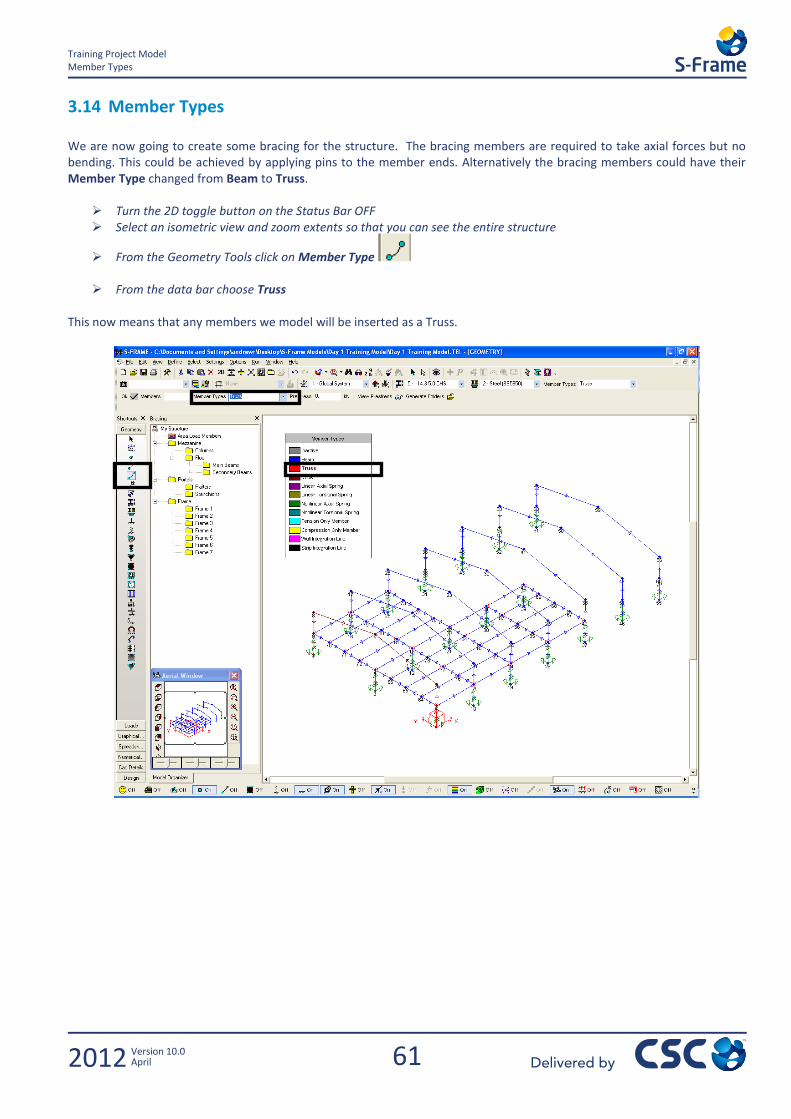
3.14 Member Types We are now going to create some bracing for the structure. The bracing members are required to take axial forces but no bending. This could be achieved by applying pins to the member ends. Alternatively the bracing members could have their Member Type changed from Beam to Truss.
Turn the 2D toggle button on the Status Bar OFF Select an isometric view and zoom extents so that you can see the entire structure
From the Geometry Tools click on Member Type
From the data bar choose Truss
This now means that any members we model will be inserted as a Truss.
62
Training Project Model Bracing
2012 Version 10.0 April
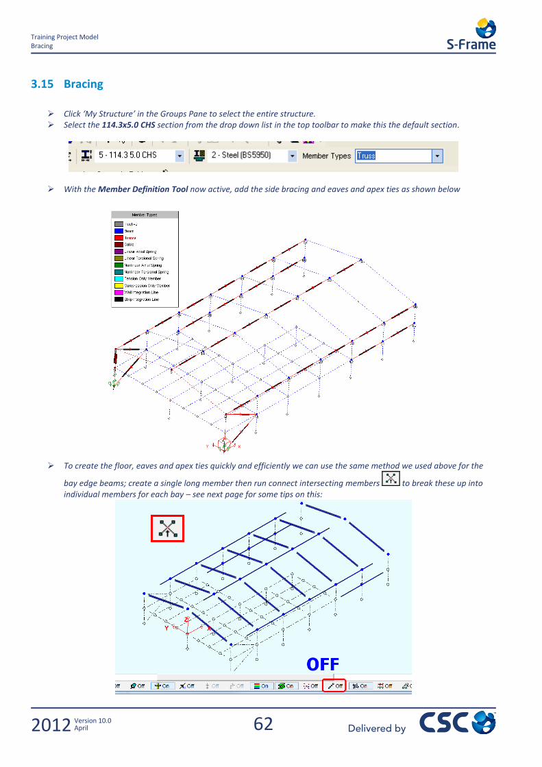
3.15 Bracing
Click ‘My Structure’ in the Groups Pane to select the entire structure. Select the 114.3x5.0 CHS section from the drop down list in the top toolbar to make this the default section.
With the Member Definition Tool now active, add the side bracing and eaves and apex ties as shown below
To create the floor, eaves and apex ties quickly and efficiently we can use the same method we used above for the
bay edge beams; create a single long member then run connect intersecting members to break these up into individual members for each bay – see next page for some tips on this:
63
Training Project Model Bracing
2012 Version 10.0 April
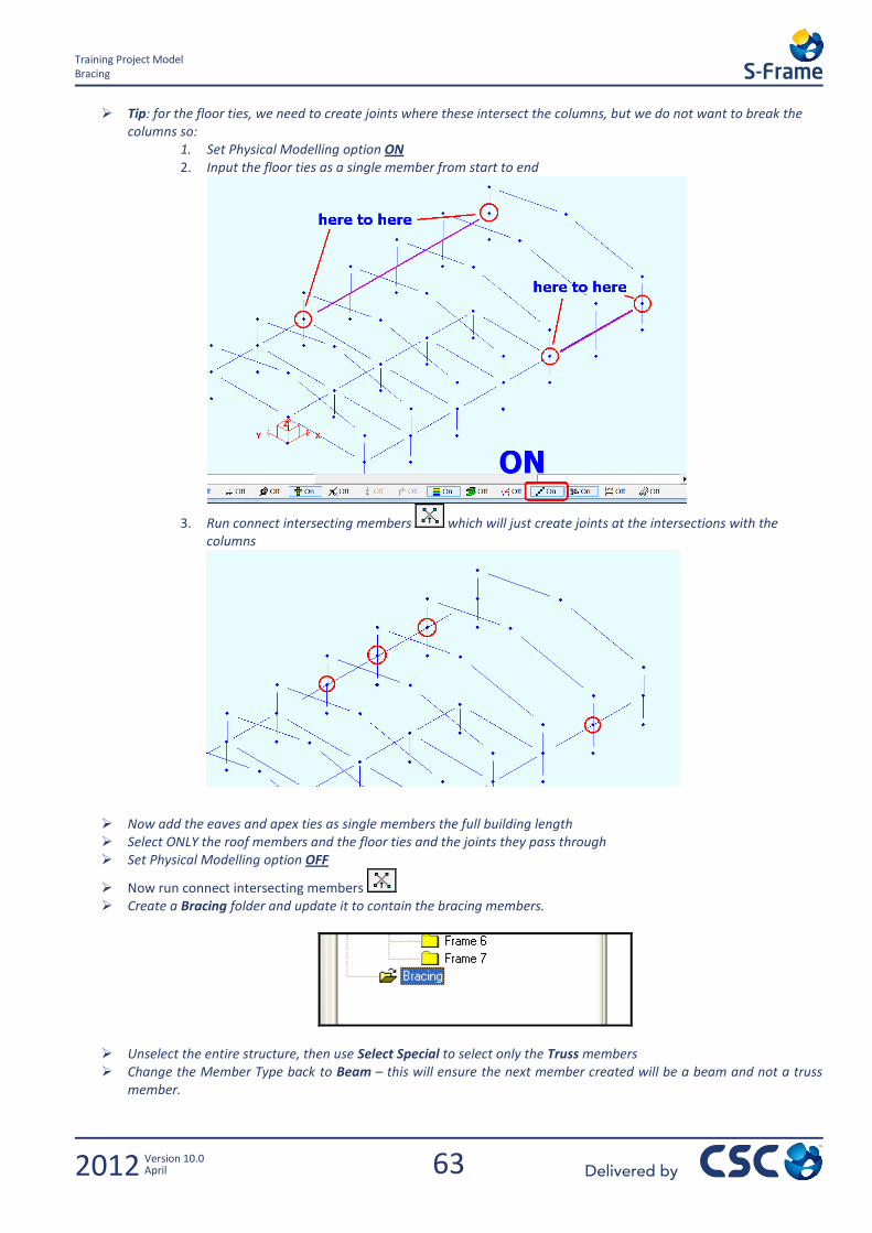
Tip: for the floor ties, we need to create joints where these intersect the columns, but we do not want to break the columns so:
1. Set Physical Modelling option ON 2. Input the floor ties as a single member from start to end
3. Run connect intersecting members which will just create joints at the intersections with the columns
Now add the eaves and apex ties as single members the full building length Select ONLY the roof members and the floor ties and the joints they pass through Set Physical Modelling option OFF
Now run connect intersecting members Create a Bracing folder and update it to contain the bracing members.
Unselect the entire structure, then use Select Special to select only the Truss members Change the Member Type back to Beam – this will ensure the next member created will be a beam and not a truss
member.
64
Training Project Model Verify & Save the Model
2012 Version 10.0 April
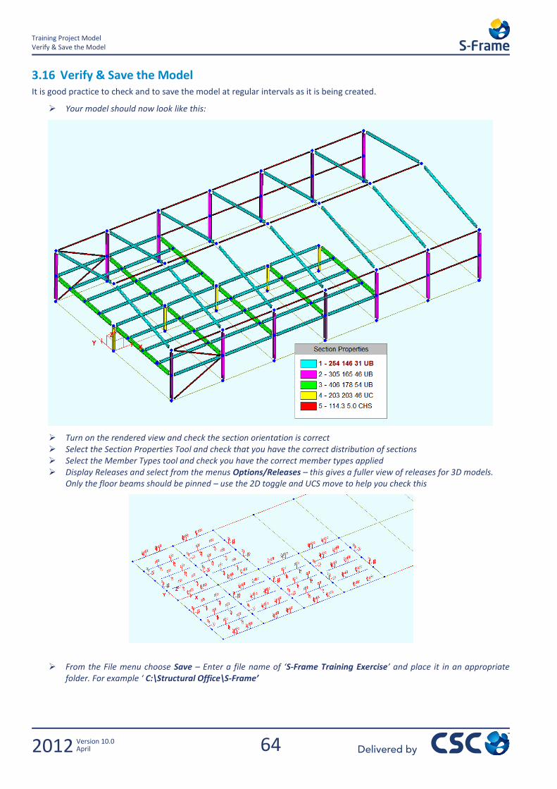
3.16 Verify & Save the Model It is good practice to check and to save the model at regular intervals as it is being created.
Your model should now look like this:
Turn on the rendered view and check the section orientation is correct Select the Section Properties Tool and check that you have the correct distribution of sections Select the Member Types tool and check you have the correct member types applied Display Releases and select from the menus Options/Releases – this gives a fuller view of releases for 3D models.
Only the floor beams should be pinned – use the 2D toggle and UCS move to help you check this
From the File menu choose Save – Enter a file name of ‘S-Frame Training Exercise’ and place it in an appropriate
folder. For example ‘ C:\Structural Office\S-Frame’
65
Training Project Model Trimming Steel
2012 Version 10.0 April
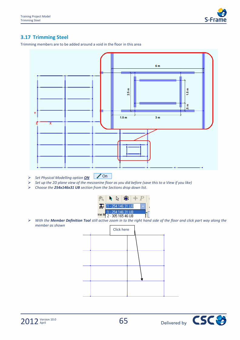
3.17 Trimming Steel Trimming members are to be added around a void in the floor in this area
Set Physical Modelling option ON Set up the 2D plane view of the mezzanine floor as you did before (save this to a View if you like) Choose the 254x146x31 UB section from the Sections drop down list.
With the Member Definition Tool still active zoom in to the right hand side of the floor and click part way along the
member as shown
Click here
66
Training Project Model Trimming Steel
2012 Version 10.0 April
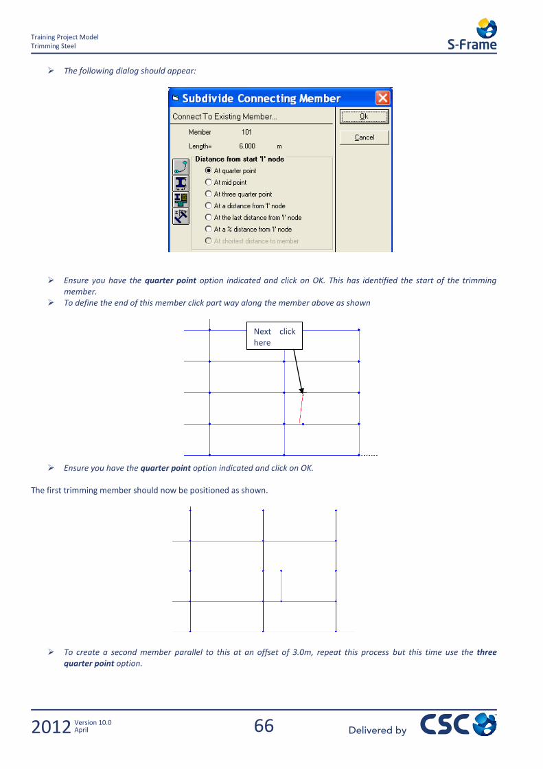
The following dialog should appear:
Ensure you have the quarter point option indicated and click on OK. This has identified the start of the trimming member.
To define the end of this member click part way along the member above as shown
Ensure you have the quarter point option indicated and click on OK.
The first trimming member should now be positioned as shown.
To create a second member parallel to this at an offset of 3.0m, repeat this process but this time use the three quarter point option.
Next click here
67
Training Project Model Trimming Steel
2012 Version 10.0 April
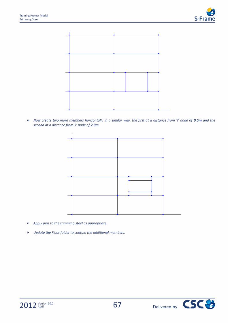
Now create two more members horizontally in a similar way, the first at a distance from ‘I’ node of 0.5m and the
second at a distance from ‘I’ node of 2.0m.
Apply pins to the trimming steel as appropriate.
Update the Floor folder to contain the additional members.


69
Rigid Diaphragms & Span Directions Trimming Steel
2012 Version 10.0 April
4.0 Rigid Diaphragms & Span Directions

71
Rigid Diaphragms & Span Directions Panels
2012 Version 10.0 April
4.1 Panels
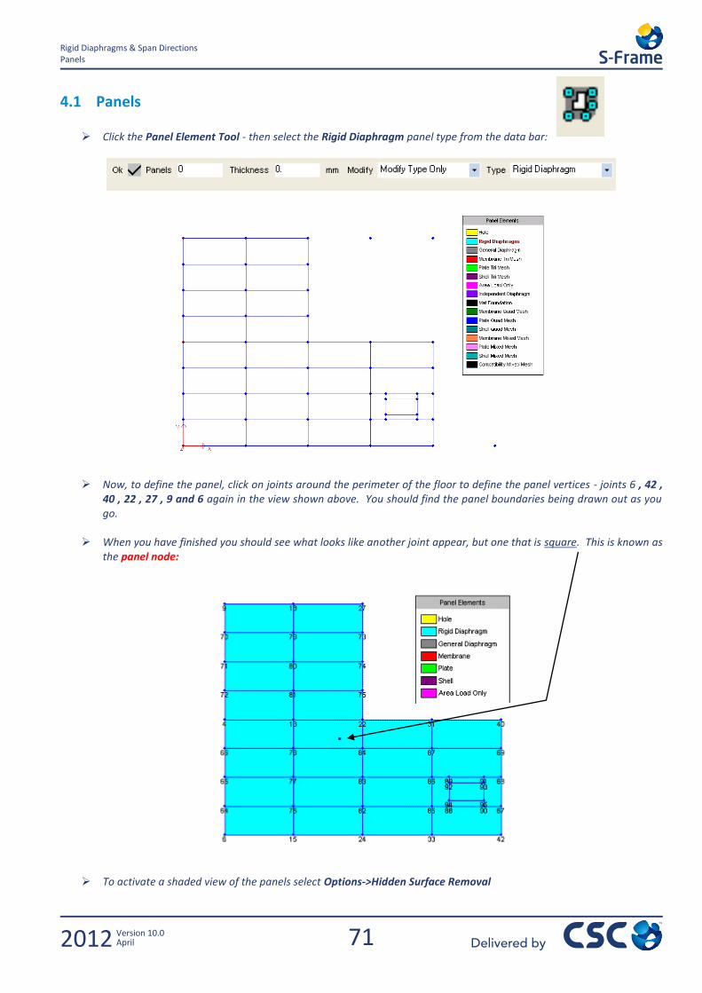
Click the Panel Element Tool - then select the Rigid Diaphragm panel type from the data bar:
Now, to define the panel, click on joints around the perimeter of the floor to define the panel vertices - joints 6 , 42 , 40 , 22 , 27 , 9 and 6 again in the view shown above. You should find the panel boundaries being drawn out as you go.
When you have finished you should see what looks like another joint appear, but one that is square. This is known as the panel node:
To activate a shaded view of the panels select Options->Hidden Surface Removal
72
Rigid Diaphragms & Span Directions Panels
2012 Version 10.0 April
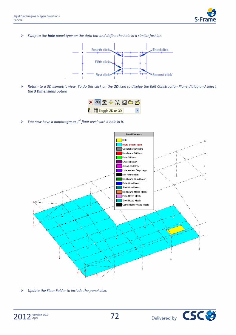
Swap to the hole panel type on the data bar and define the hole in a similar fashion.
Return to a 3D isometric view. To do this click on the 2D icon to display the Edit Construction Plane dialog and select the 3 Dimensions option
You now have a diaphragm at 1st
floor level with a hole in it.
Update the Floor Folder to include the panel also.
73
Rigid Diaphragms & Span Directions Span Direction
2012 Version 10.0 April
4.2 Span Direction A span direction can be assigned to rigid diaphragm or area load panels if required. This direction is then used to determine how area loads will be decomposed to the supporting members Following are the basic steps required to set the span direction.
1. Create a Panel over the area you wish to apply the load 2. Add the members which will take the area load to the Area Load folder 3. Set the spanning direction for the panel
4.2.1 Creating the Panel
In this example, a panel has already been created to define the rigid diaphragm. The same panel can be used to apply the area load.
4.2.2 Area Load Members Folder
All the members on to which the area load will be decomposed are currently in the Floors folder. We will COPY the contents of this folder to the Area Load Member folder:
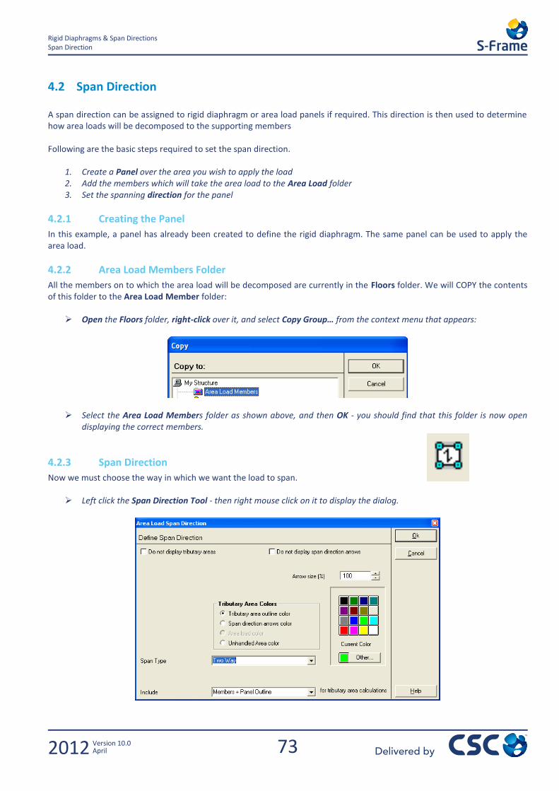
Open the Floors folder, right-click over it, and select Copy Group… from the context menu that appears:
Select the Area Load Members folder as shown above, and then OK - you should find that this folder is now open displaying the correct members.
4.2.3 Span Direction
Now we must choose the way in which we want the load to span.
Left click the Span Direction Tool - then right mouse click on it to display the dialog.
74
Rigid Diaphragms & Span Directions Span Direction
2012 Version 10.0 April
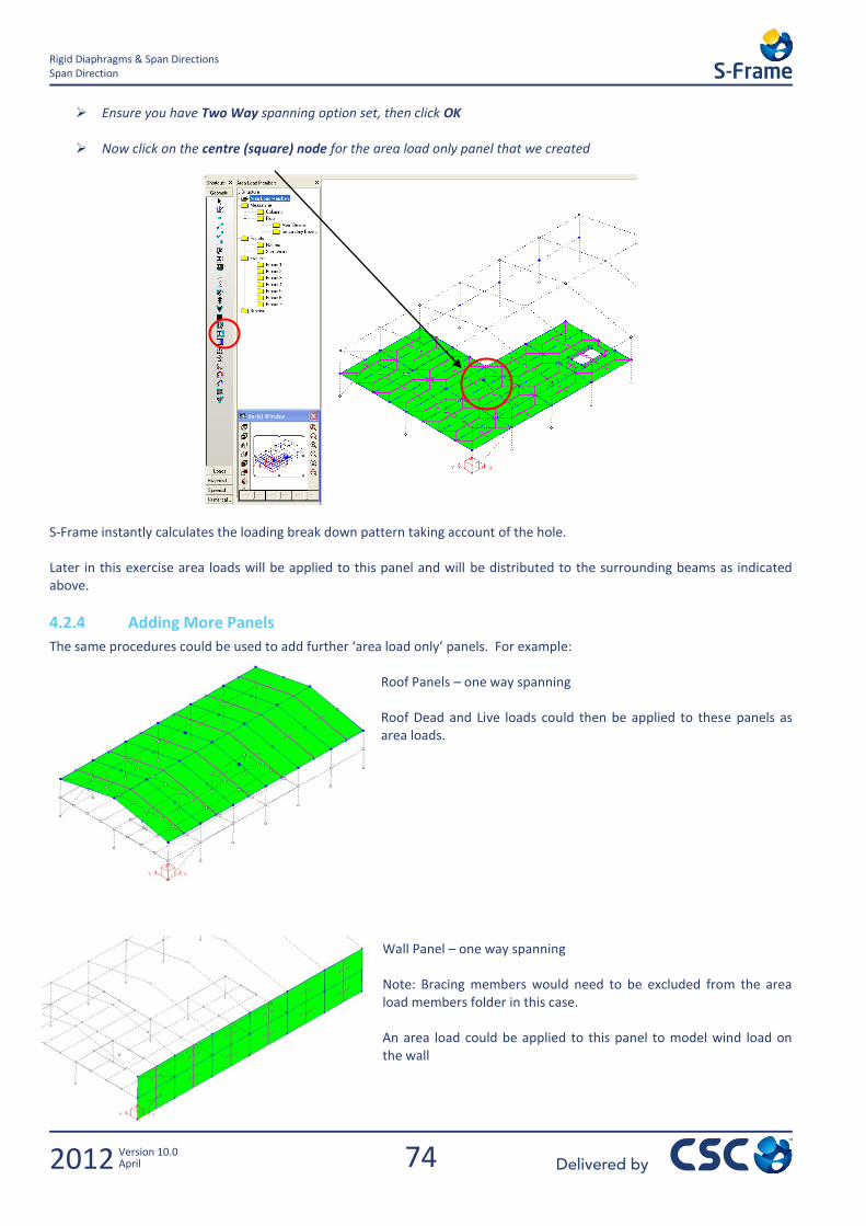
Ensure you have Two Way spanning option set, then click OK
Now click on the centre (square) node for the area load only panel that we created
S-Frame instantly calculates the loading break down pattern taking account of the hole. Later in this exercise area loads will be applied to this panel and will be distributed to the surrounding beams as indicated above.
4.2.4 Adding More Panels
The same procedures could be used to add further ‘area load only’ panels. For example: Roof Panels – one way spanning Roof Dead and Live loads could then be applied to these panels as area loads.
Wall Panel – one way spanning Note: Bracing members would need to be excluded from the area load members folder in this case. An area load could be applied to this panel to model wind load on the wall

75
The Loads Window Span Direction
2012 Version 10.0 April
5.0 The Loads Window


77
The Loads Window Unfactored Loadcases
2012 Version 10.0 April
5.1 Unfactored Loadcases The following five load cases will be created:
1. Roof Dead 2. Roof Live 3. Self Weight. 4. Floor Dead 5. Floor Live
The first two load cases will be created as Global Projected Member Loads using the Loads Toolbar. The structure self weight is a special case and is created by specifying a Gravity Factor. The floor load cases will be created using the area loads feature:
Click on the Loads button in the bottom left corner of the screen to view to the Loads window. Once viewed, these windows can be accessed through the Window drop down menu.
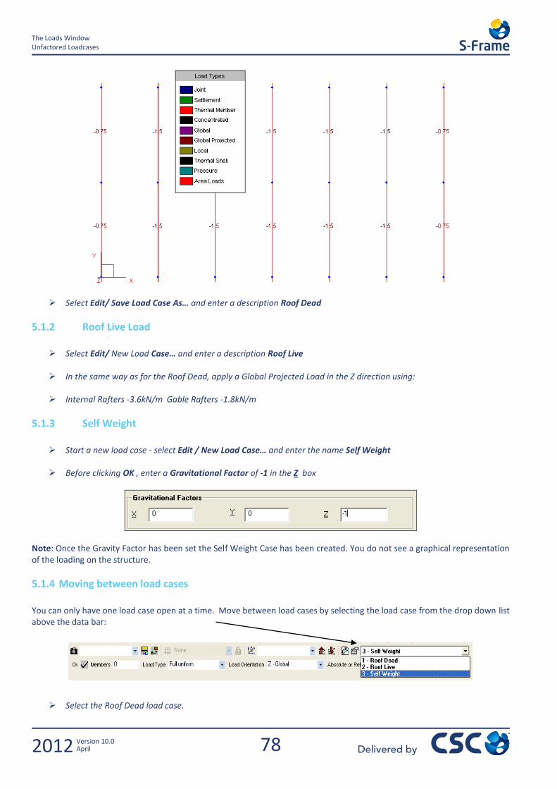
5.1.1 Roof Dead Load
Click the Global Projected Load button
In the data bar select Z-Global from the drop down list.
Enter the load value of -1.5 kN/m in the data bar
Instead of clicking on each rafter individually to apply the load, careful use of the Member Group Folders and the Aerial Window can speed up this operation.
Select only the rafters by opening the appropriate Group Folder.
From the Aerial Window choose a Top View.
From the Status Bar, Hide Unselected Members
Apply the load to all the internal rafters by boxing around them.
Change the load value to -0.75 kN/m in the data bar
Apply the new load to the gable rafters by boxing around them, the screen should look as follows:
78
The Loads Window Unfactored Loadcases
2012 Version 10.0 April
Select Edit/ Save Load Case As… and enter a description Roof Dead
5.1.2 Roof Live Load
Select Edit/ New Load Case… and enter a description Roof Live
In the same way as for the Roof Dead, apply a Global Projected Load in the Z direction using:
Internal Rafters -3.6kN/m Gable Rafters -1.8kN/m
5.1.3 Self Weight
Start a new load case - select Edit / New Load Case… and enter the name Self Weight Before clicking OK , enter a Gravitational Factor of -1 in the Z box
Note: Once the Gravity Factor has been set the Self Weight Case has been created. You do not see a graphical representation of the loading on the structure.
5.1.4 Moving between load cases
You can only have one load case open at a time. Move between load cases by selecting the load case from the drop down list above the data bar:
Select the Roof Dead load case.

79
The Loads Window Unfactored Loadcases
2012 Version 10.0 April
Enable permanent viewing of all Member Loads by clicking the Member Loads button on the Status toolbar at the
bottom of the window:
You can do the same with Joint Loads
With this setting you can view all loads applied irrespective of which loads tool is selected.
Practice moving between load cases
You move between load cases and combinations in the same way when viewing Results.

80
The Loads Window Applying an Area Load
2012 Version 10.0 April
5.2 Applying an Area Load
From the Edit menu choose New Load case and enter the load description as Floor Dead.
If necessary select an Isometric View and zoom extents and select all.
Ensure you switch Member Loads On on the Status Bar.
Now select the Area Load Tool and enter a load of -0.8 kN/m2 magnitude, in the Global Z direction.
Finally, click on the Panel’s central node - you will see that S-Frame adds the load and also shows the distribution pattern:
From the Edit menu choose New Load case and enter the load description as Floor Live.
Still using the Area Load Tool and enter a magnitude value of -2.5 kN/m2 in the Global Z direction.
Click on the Panel’s central node – once again you will see that S-Frame adds the load and also shows the
distribution pattern:
81
The Loads Window Applying an Area Load
2012 Version 10.0 April
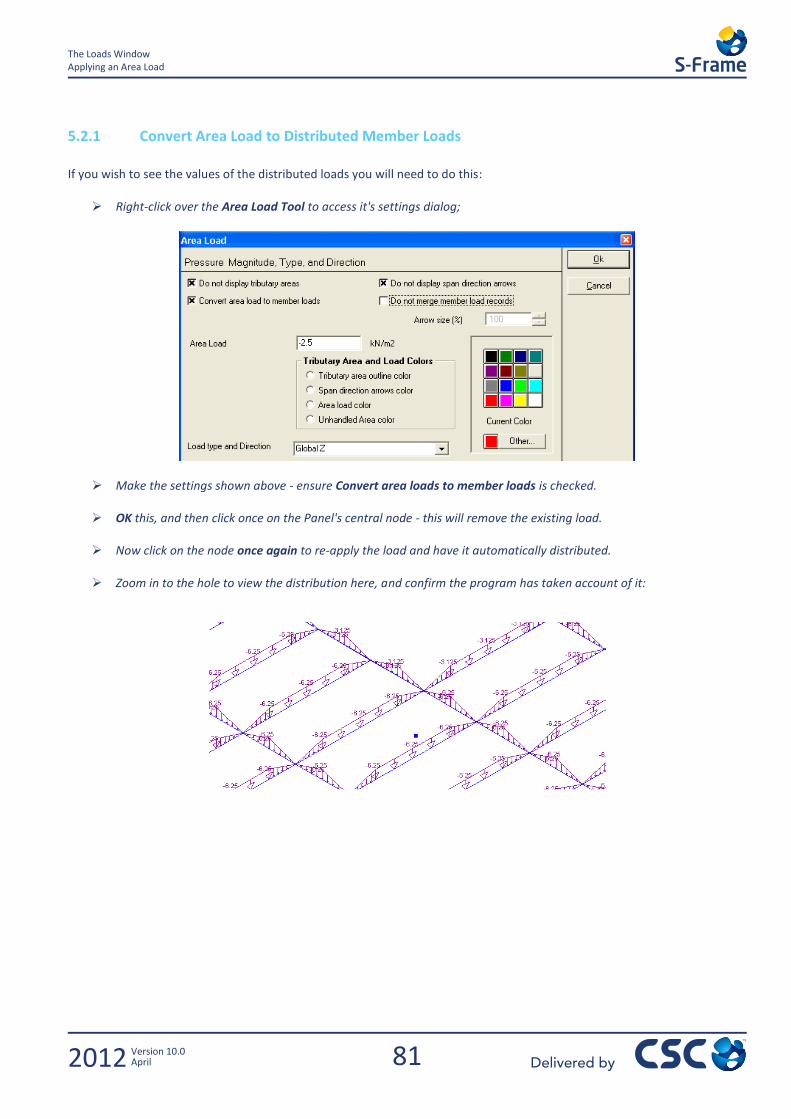
5.2.1 Convert Area Load to Distributed Member Loads
If you wish to see the values of the distributed loads you will need to do this:
Right-click over the Area Load Tool to access it's settings dialog;
Make the settings shown above - ensure Convert area loads to member loads is checked.
OK this, and then click once on the Panel's central node - this will remove the existing load.
Now click on the node once again to re-apply the load and have it automatically distributed.
Zoom in to the hole to view the distribution here, and confirm the program has taken account of it:
82
The Loads Window Creating Load Combinations
2012 Version 10.0 April
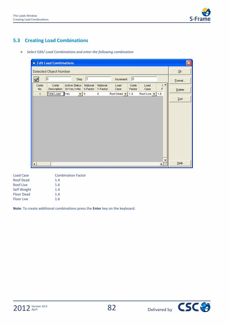
5.3 Creating Load Combinations
Select Edit/ Load Combinations and enter the following combination
Load Case Combination Factor Roof Dead 1.4 Roof Live 1.6 Self Weight 1.4 Floor Dead 1.4 Floor Live 1.6 Note: To create additional combinations press the Enter key on the keyboard.

83
The Loads Window Creating Load Combinations
2012 Version 10.0 April


85
Analysis & Results Creating Load Combinations
2012 Version 10.0 April
6.0 Analysis & Results


87
Analysis & Results Analysis Check List
2012 Version 10.0 April
6.1 Analysis Check List The structure is now ready for analysis but before analysing for the first time it is a good idea to run through the following check list and ensure that all the required aspects of the structure have been entered:
1. Have you added all the required members - do you have any Stray Nodes? (Hint use Zoom Extents to ensure all members and joints are displayed. Use File/ Integrity Checks… to search for stray nodes)
2. Have you connected your model correctly - remember if a member passes through a joint or another member it is
not connected to that joint or member. ( Hint - again use File/ Integrity Checks…)
3. Have you applied Member Releases to the model appropriate to the connections in your structure or your
engineering assumptions (e.g. all bracing assumed pin-ended). ( Hint - turn on viewing of releases permanently)
4. Have you applied Supports to the structure
( Hint - turn on viewing of supports permanently)
5. Does your structure look Stable? Have you introduced any mechanisms by applying too many releases or omitting bracing elements.
6. Have you applied Sections to All the members and are they applied correctly?
( Hint - click the Section Properties Tool button in the Geometry window)
7. Have you applied Materials to All members and are they applied correctly? ( Hint - click the Material Properties Tool button in the Geometry window)
8. Have you applied loads to the structure?
( Hint - Select the Loads window and examine your load cases)
9. Have you created load combinations if you want to look at the combined effects of more than one load case.
If you have omitted some of the above you are likely to get either error messages or warnings. If you do get warnings or errors then run through the above check list again. You are advised to ascertain the reason for these and remedy any problems to achieve an analysis with no warnings or errors.
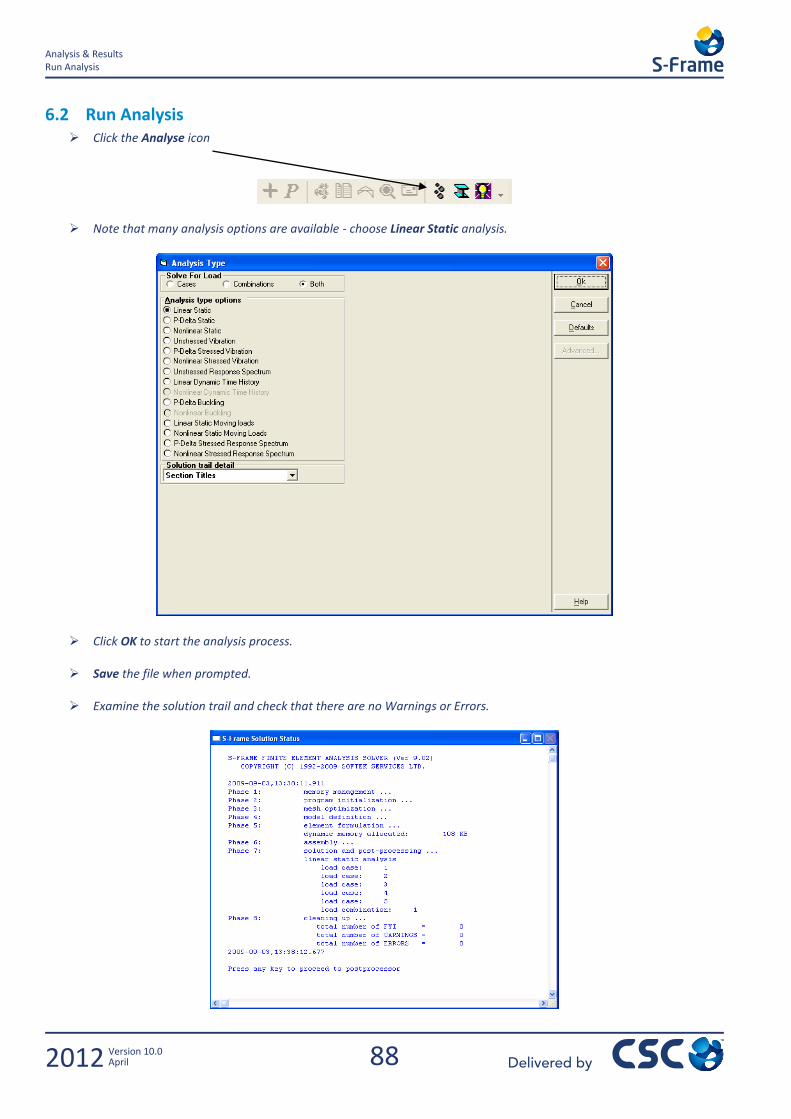
88
Analysis & Results Run Analysis
2012 Version 10.0 April
6.2 Run Analysis Click the Analyse icon
Note that many analysis options are available - choose Linear Static analysis.
Click OK to start the analysis process.
Save the file when prompted.
Examine the solution trail and check that there are no Warnings or Errors.
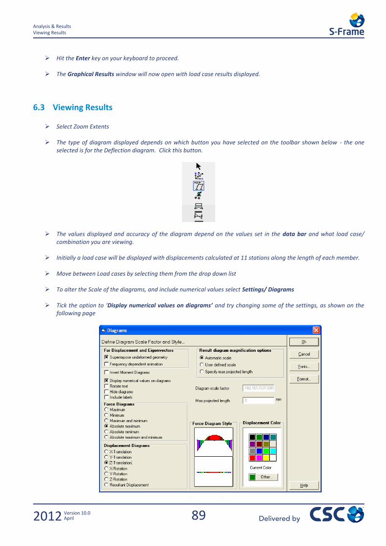
89
Analysis & Results Viewing Results
2012 Version 10.0 April
Hit the Enter key on your keyboard to proceed.
The Graphical Results window will now open with load case results displayed.
6.3 Viewing Results
Select Zoom Extents
The type of diagram displayed depends on which button you have selected on the toolbar shown below - the one selected is for the Deflection diagram. Click this button.
The values displayed and accuracy of the diagram depend on the values set in the data bar and what load case/ combination you are viewing.
Initially a load case will be displayed with displacements calculated at 11 stations along the length of each member.
Move between Load cases by selecting them from the drop down list
To alter the Scale of the diagrams, and include numerical values select Settings/ Diagrams
Tick the option to ‘Display numerical values on diagrams’ and try changing some of the settings, as shown on the following page
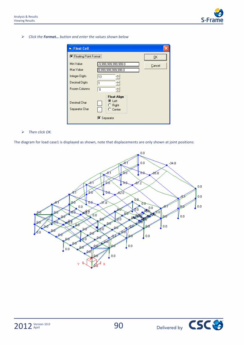
90
Analysis & Results Viewing Results
2012 Version 10.0 April
Click the Format… button and enter the values shown below
Then click OK. The diagram for load case1 is displayed as shown, note that displacements are only shown at joint positions:
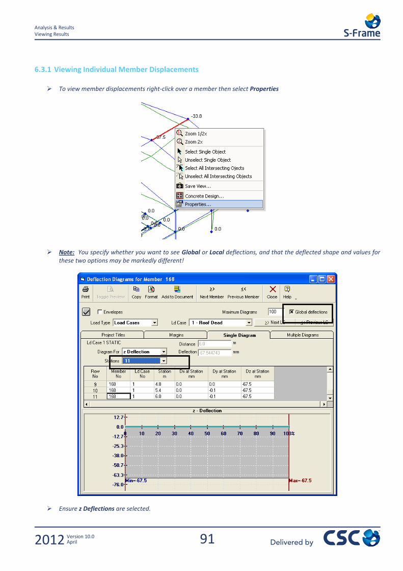
91
Analysis & Results Viewing Results
2012 Version 10.0 April
6.3.1 Viewing Individual Member Displacements
To view member displacements right-click over a member then select Properties
Note: You specify whether you want to see Global or Local deflections, and that the deflected shape and values for these two options may be markedly different!
Ensure z Deflections are selected.
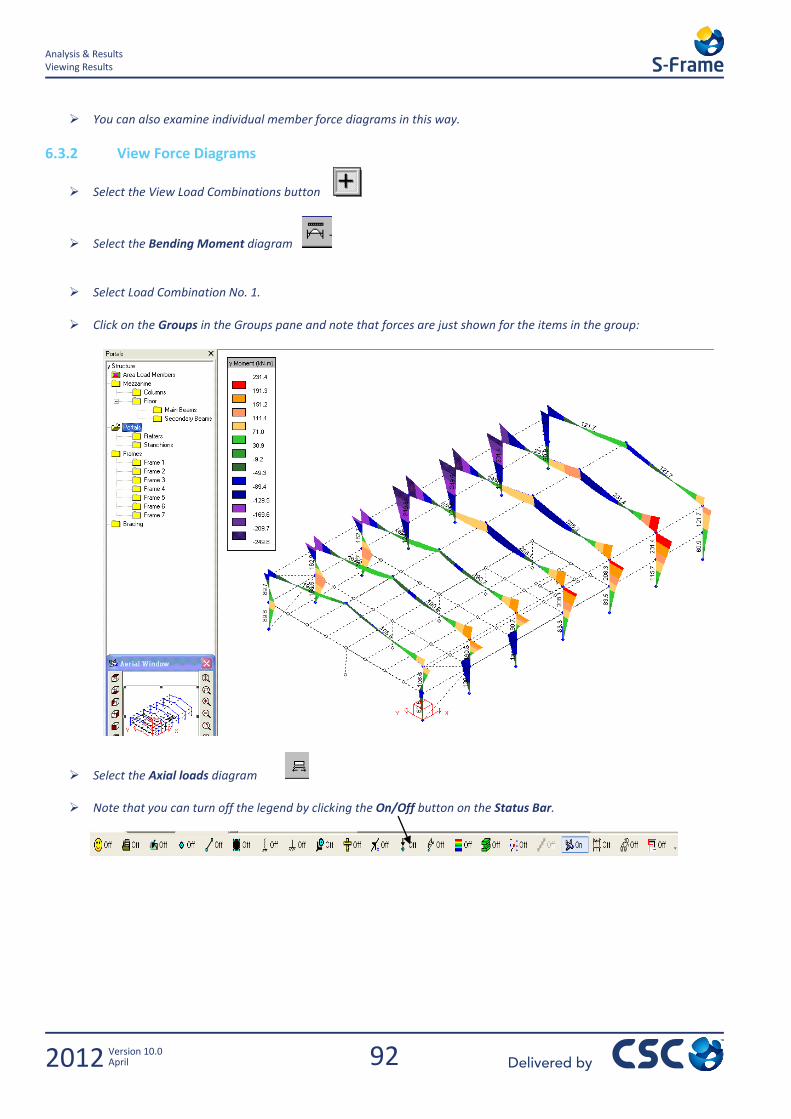
92
Analysis & Results Viewing Results
2012 Version 10.0 April
You can also examine individual member force diagrams in this way.
6.3.2 View Force Diagrams
Select the View Load Combinations button
Select the Bending Moment diagram
Select Load Combination No. 1.
Click on the Groups in the Groups pane and note that forces are just shown for the items in the group:
Select the Axial loads diagram
Note that you can turn off the legend by clicking the On/Off button on the Status Bar.
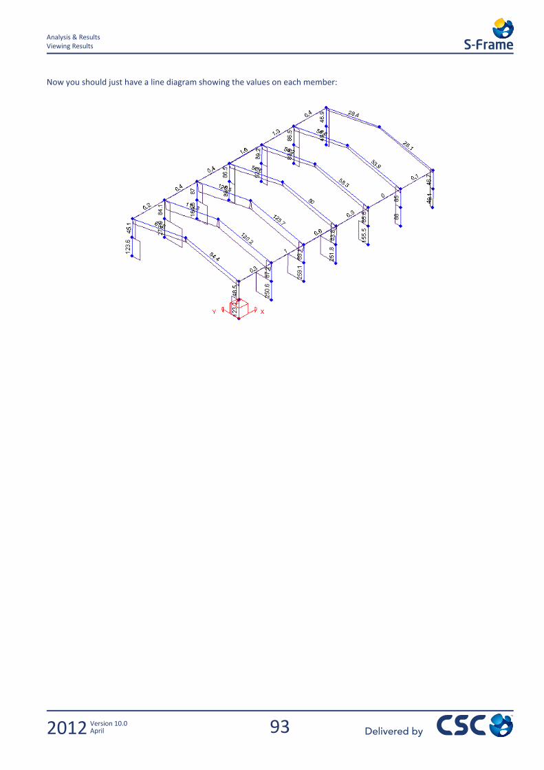
93
Analysis & Results Viewing Results
2012 Version 10.0 April
Now you should just have a line diagram showing the values on each member:


95
Output Viewing Results
2012 Version 10.0 April
7.0 Output

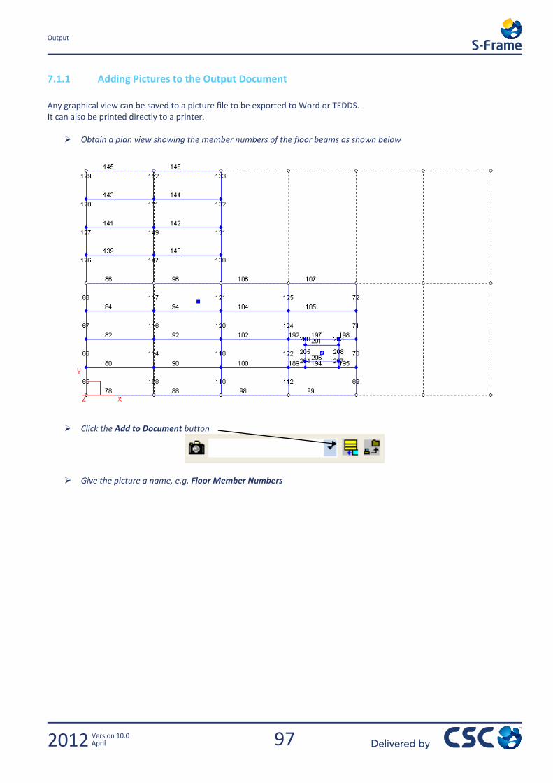
97
Output
2012 Version 10.0 April
7.1.1 Adding Pictures to the Output Document
Any graphical view can be saved to a picture file to be exported to Word or TEDDS. It can also be printed directly to a printer.
Obtain a plan view showing the member numbers of the floor beams as shown below
Click the Add to Document button
Give the picture a name, e.g. Floor Member Numbers

98
Output
2012 Version 10.0 April
Obtain a graphical view showing the Z deflections on the Floor Main Beams due to Imposed Load as shown below
Click the Add to Document button
Give the picture a name, e.g. Floor Live Load Deflections
7.1.2 Adding Reports to the Output Document
Reports can also be created and added to the file for export to Word or TEDDS. The Reports can also be printed directly to a printer.
Select the Numerical Results tab
Click on either the buttons on the left hand side tool bar, or on the tabs at the bottom of the screen to view various different results.
Note: If you right click on any of the buttons on the left hand side tool bar a Spreadsheet Components window will
appear, allowing you to filter which columns you want displayed in the spreadsheet.
Click the Add to Document button again and enter a title: e.g. Factored Floor Design Forces
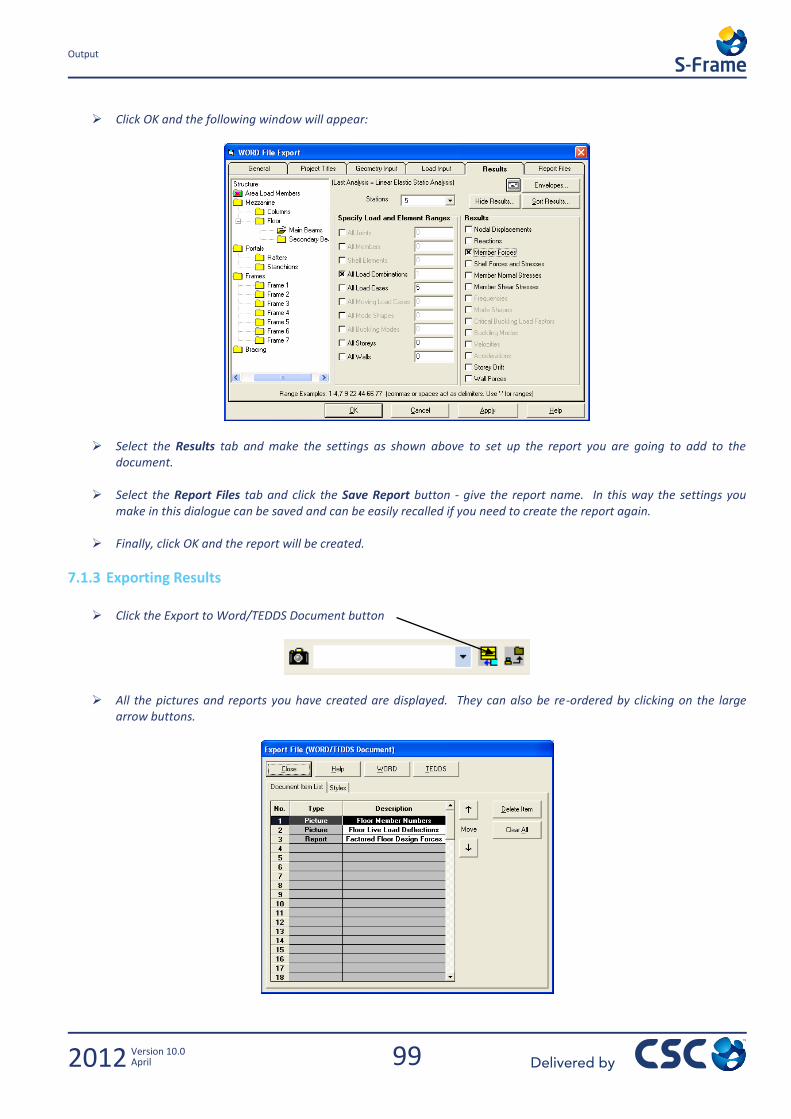
99
Output
2012 Version 10.0 April
Click OK and the following window will appear:
Select the Results tab and make the settings as shown above to set up the report you are going to add to the document.
Select the Report Files tab and click the Save Report button - give the report name. In this way the settings you make in this dialogue can be saved and can be easily recalled if you need to create the report again.
Finally, click OK and the report will be created.
7.1.3 Exporting Results
Click the Export to Word/TEDDS Document button
All the pictures and reports you have created are displayed. They can also be re-ordered by clicking on the large arrow buttons.

100
Output
2012 Version 10.0 April
Click the Word button to export the report to Word.

101
Introduction to FE Analysis
2012 Version 10.0 April
8.0 Introduction to FE Analysis


103
Introduction to FE Analysis Introduction
2012 Version 10.0 April
8.1 Introduction S-Frame supports the use of ‘2D’ quadrilateral (quad) and triangular (tri) finite elements in all versions of S-Frame. Although technically speaking all the member types are finite elements it is common parlance to apply the term FE to these 2D elements. Analysis using FE elements requires a more extensive knowledge of the effects of modelling than simple frame analysis. As such, this simple example is not intended to cover the wider topic of FE analysis but simply to inform of the method of application of the elements in a very simple model. Users who wish to use S-Frame for FE analysis should attend the additional S-Frame FE analysis training course which spends a day working through the issues associated with FE analysis. In addition, users wishing to design concrete flat slabs using FE analysis should study the extensive background reading available, such as ‘How to design reinforced concrete flat slabs using Finite Element Analysis’ written by O Brooker for the Concrete Centre. Studying of such material should be considered essential. S-Frame uses a sophisticated 2D element called the ‘Mindlin Resisler thick shell element’ which gives excellent results under both linear elastic and second order analysis, but as with all FE analysis the results are subject to effective meshing AND, importantly, the correct use of material properties. In our simple example, we will use a common section property in order to illustrate the issues of comparative analysis – the material properties we use in this example should not be taken as guidance on the material properties you should use.
O Brooker says;
“The choice of elastic modulus is particularly critical when using linear FE analysis to check serviceability criteria.”
“Deflection is influenced by many factors, including the tensile and compressive strength of the concrete, the elastic modulus, shrinkage, creep, ambient conditions, restraint, loading, time, duration of loading and cracking. With so many influences, and many which are difficult to accurately predict, the deflection calculations should be regarded as an estimate only. The Concrete Society report ‘Deflections in concrete slabs and beams’ advises that the difference between calculated and actual deflections falls in the range +15% to -30%.” “In general, the long-term elastic modulus is usually between a third (for storage loads) and a half (for residential loads) of the short term value. Therefore allowing for the need to adjust for cracked stiffness, the long term elastic modulus should be in the range one sixth ( x 0.167) to one quarter ( x 0.25) of the short term modulus.”
Users who are using Eurocodes should pay close attention to:
BS EN 1992-1-1:2004 clause 5.8.7.2 and Annex H
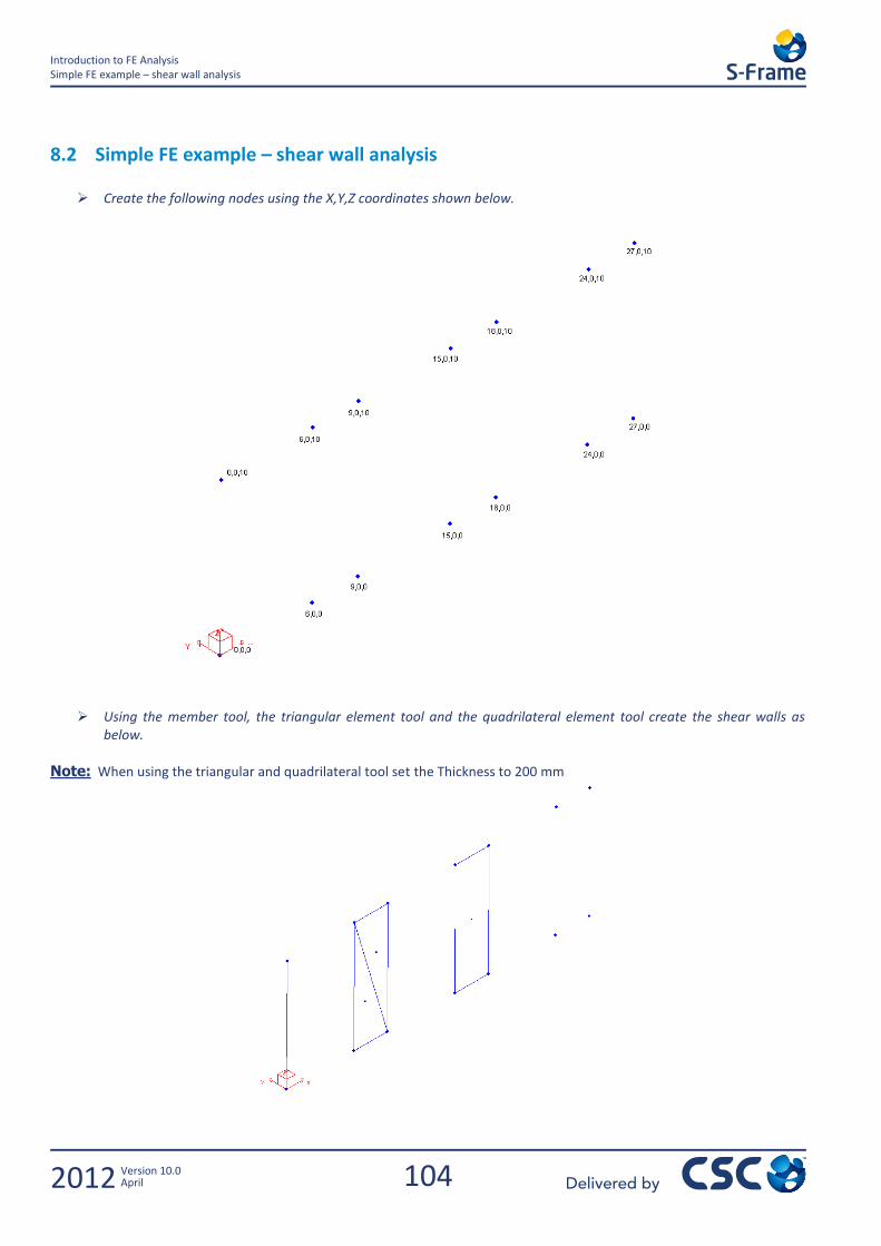
104
Introduction to FE Analysis Simple FE example – shear wall analysis
2012 Version 10.0 April
8.2 Simple FE example – shear wall analysis
Create the following nodes using the X,Y,Z coordinates shown below.
Using the member tool, the triangular element tool and the quadrilateral element tool create the shear walls as
below.
Note: When using the triangular and quadrilateral tool set the Thickness to 200 mm
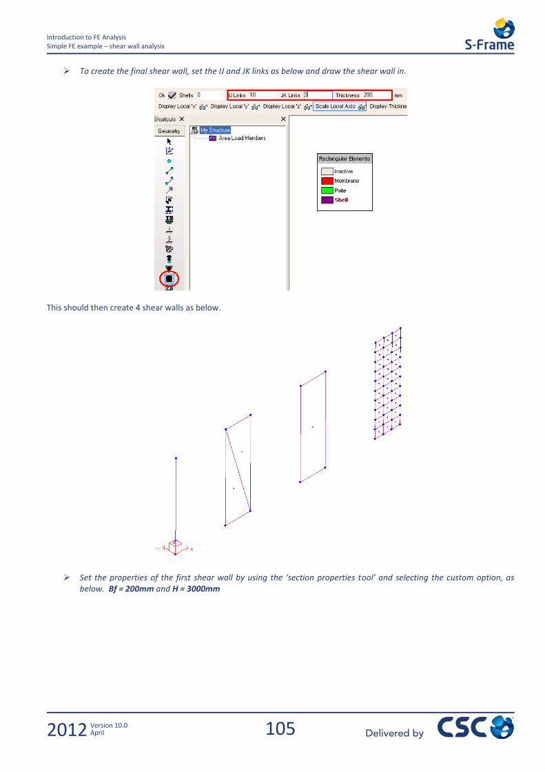
105
Introduction to FE Analysis Simple FE example – shear wall analysis
2012 Version 10.0 April
To create the final shear wall, set the IJ and JK links as below and draw the shear wall in.
This should then create 4 shear walls as below.
Set the properties of the first shear wall by using the ‘section properties tool’ and selecting the custom option, as below. Bf = 200mm and H = 3000mm
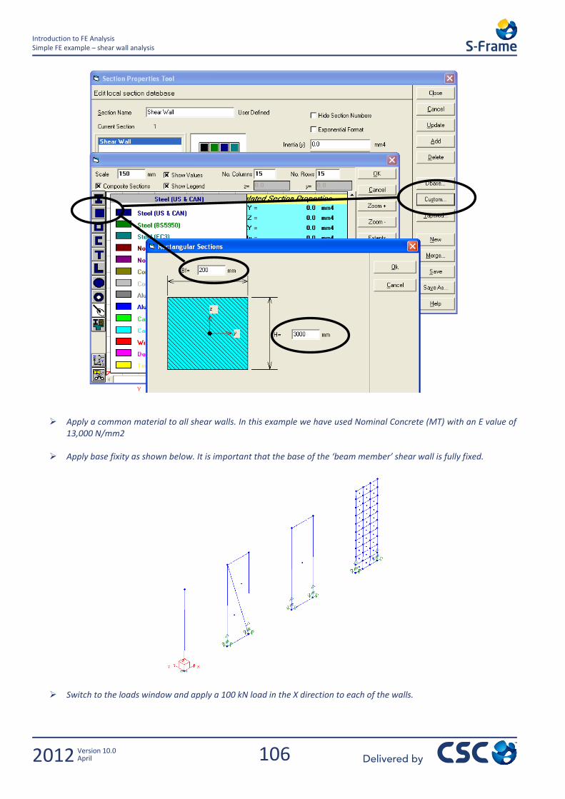
106
Introduction to FE Analysis Simple FE example – shear wall analysis
2012 Version 10.0 April
Apply a common material to all shear walls. In this example we have used Nominal Concrete (MT) with an E value of 13,000 N/mm2
Apply base fixity as shown below. It is important that the base of the ‘beam member’ shear wall is fully fixed.
Switch to the loads window and apply a 100 kN load in the X direction to each of the walls.
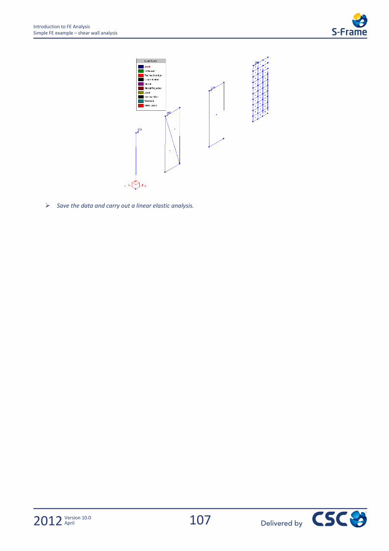
107
Introduction to FE Analysis Simple FE example – shear wall analysis
2012 Version 10.0 April
Save the data and carry out a linear elastic analysis.
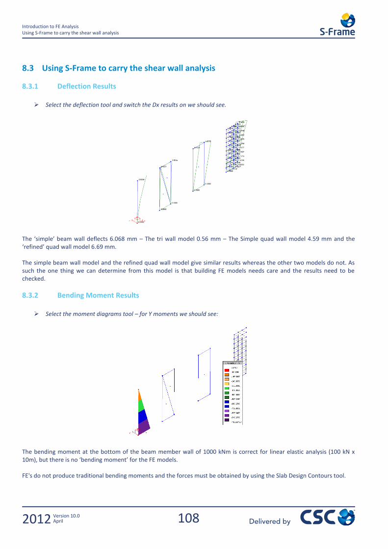
108
Introduction to FE Analysis Using S-Frame to carry the shear wall analysis
2012 Version 10.0 April
8.3 Using S-Frame to carry the shear wall analysis
8.3.1 Deflection Results
Select the deflection tool and switch the Dx results on we should see.
The ‘simple’ beam wall deflects 6.068 mm – The tri wall model 0.56 mm – The Simple quad wall model 4.59 mm and the ‘refined’ quad wall model 6.69 mm. The simple beam wall model and the refined quad wall model give similar results whereas the other two models do not. As such the one thing we can determine from this model is that building FE models needs care and the results need to be checked.
8.3.2 Bending Moment Results
Select the moment diagrams tool – for Y moments we should see:
The bending moment at the bottom of the beam member wall of 1000 kNm is correct for linear elastic analysis (100 kN x 10m), but there is no ‘bending moment’ for the FE models. FE's do not produce traditional bending moments and the forces must be obtained by using the Slab Design Contours tool.
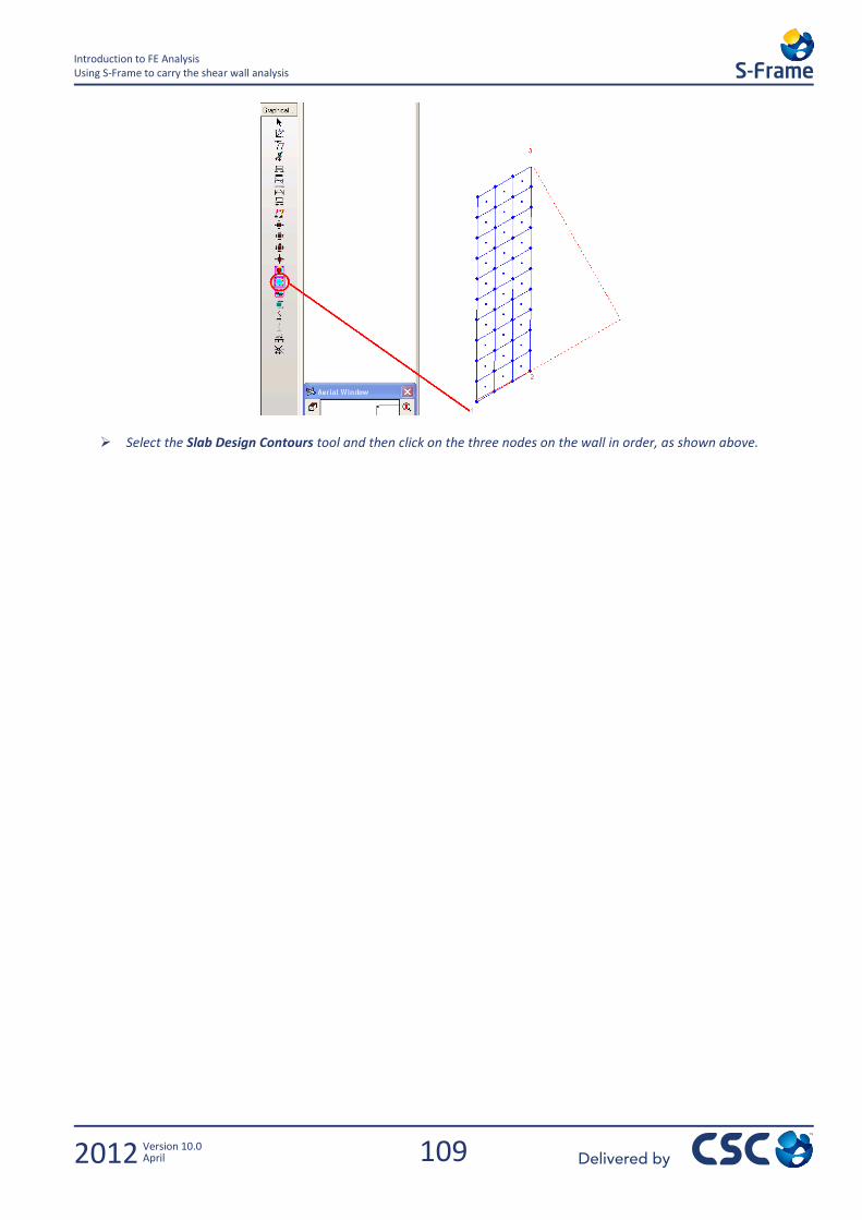
109
Introduction to FE Analysis Using S-Frame to carry the shear wall analysis
2012 Version 10.0 April
Select the Slab Design Contours tool and then click on the three nodes on the wall in order, as shown above.
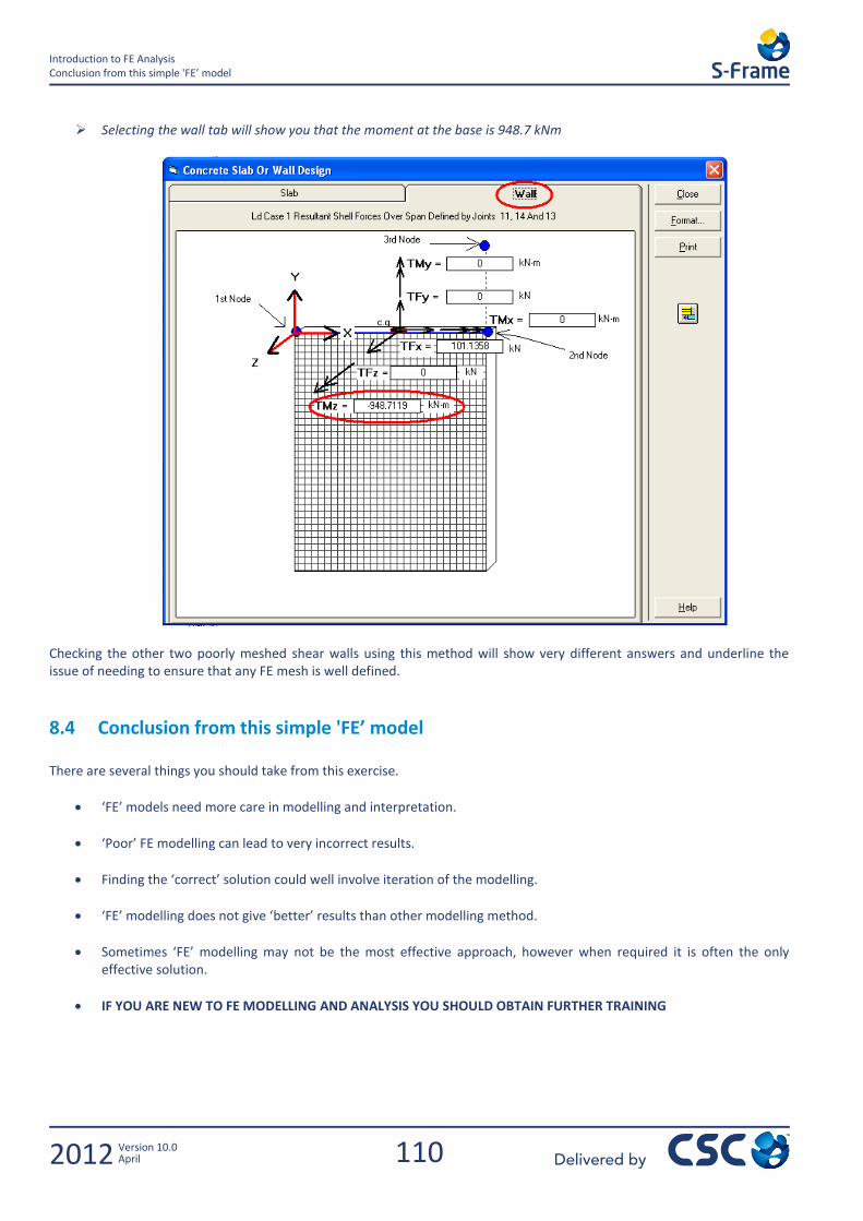
110
Introduction to FE Analysis Conclusion from this simple 'FE’ model
2012 Version 10.0 April
Selecting the wall tab will show you that the moment at the base is 948.7 kNm
Checking the other two poorly meshed shear walls using this method will show very different answers and underline the issue of needing to ensure that any FE mesh is well defined.
8.4 Conclusion from this simple 'FE’ model There are several things you should take from this exercise.
‘FE’ models need more care in modelling and interpretation.
‘Poor’ FE modelling can lead to very incorrect results.
Finding the ‘correct’ solution could well involve iteration of the modelling.
‘FE’ modelling does not give ‘better’ results than other modelling method.
Sometimes ‘FE’ modelling may not be the most effective approach, however when required it is often the only effective solution.
IF YOU ARE NEW TO FE MODELLING AND ANALYSIS YOU SHOULD OBTAIN FURTHER TRAINING

111
Sway Checks & P-Delta Analysis Conclusion from this simple 'FE’ model
2012 Version 10.0 April
9.0 Sway Checks & P-Delta Analysis

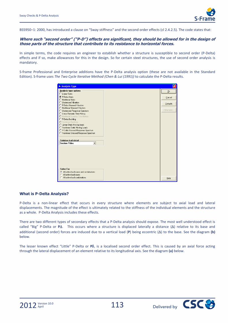
113
Sway Checks & P-Delta Analysis
2012 Version 10.0 April
BS5950–1: 2000, has introduced a clause on “Sway stiffness” and the second order effects (cl 2.4.2.5). The code states that:
Where such “second order” (“P-D”) effects are significant, they should be allowed for in the design of those parts of the structure that contribute to its resistance to horizontal forces. In simple terms, the code requires an engineer to establish whether a structure is susceptible to second order (P-Delta) effects and if so, make allowances for this in the design. So for certain steel structures, the use of second order analysis is mandatory. S-frame Professional and Enterprise additions have the P-Delta analysis option (these are not available in the Standard Edition). S-frame uses The Two Cycle Iterative Method (Chen & Lui (1991)) to calculate the P-Delta results.
What is P-Delta Analysis?
P-Delta is a non-linear effect that occurs in every structure where elements are subject to axial load and lateral displacements. The magnitude of the effect is ultimately related to the stiffness of the individual elements and the structure as a whole. P-Delta Analysis includes these effects. There are two different types of secondary effects that a P-Delta analysis should expose. The most well understood effect is
called “Big” P-Delta or P. This occurs where a structure is displaced laterally a distance () relative to its base and
additional (second order) forces are induced due to a vertical load (P) being eccentric () to the base. See the diagram (b) below.
The lesser known effect “Little” P-Delta or P, is a localised second order effect. This is caused by an axial force acting through the lateral displacement of an element relative to its longitudinal axis. See the diagram (a) below.
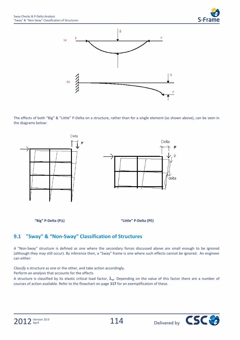
114
Sway Checks & P-Delta Analysis "Sway" & “Non-Sway” Classification of Structures
2012 Version 10.0 April
The effects of both “Big” & “Little” P-Delta on a structure, rather than for a single element (as shown above), can be seen in the diagrams below:
“Big” P-Delta (P) “Little” P-Delta (P)
9.1 "Sway" & “Non-Sway” Classification of Structures A “Non-Sway” structure is defined as one where the secondary forces discussed above are small enough to be ignored (although they may still occur). By inference then, a "Sway" frame is one where such effects cannot be ignored. An engineer can either: Classify a structure as one or the other, and take action accordingly. Perform an analysis that accounts for the effects
A structure is classified by its elastic critical load factor, cr. Depending on the value of this factor there are a number of
courses of action available. Refer to the flowchart on page 117 for an exemplification of these.
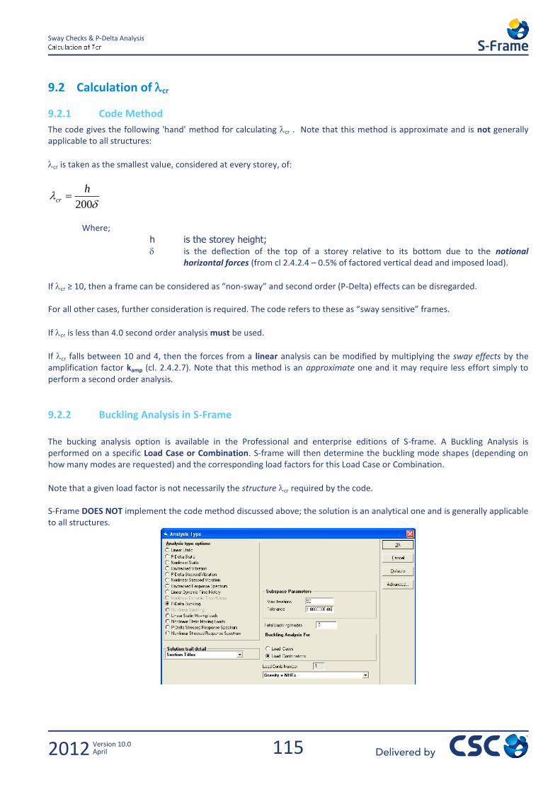
115
Sway Checks & P-Delta Analysis
2012 Version 10.0 April
9.2 Calculation of cr
9.2.1 Code Method
The code gives the following 'hand' method for calculating cr . Note that this method is approximate and is not generally applicable to all structures:
cr is taken as the smallest value, considered at every storey, of:
200
hcr
Where;
h is the storey height;
is the deflection of the top of a storey relative to its bottom due to the notional horizontal forces (from cl 2.4.2.4 – 0.5% of factored vertical dead and imposed load).
If cr ≥ 10, then a frame can be considered as “non-sway” and second order (P-Delta) effects can be disregarded. For all other cases, further consideration is required. The code refers to these as “sway sensitive” frames.
If cr is less than 4.0 second order analysis must be used.
If cr falls between 10 and 4, then the forces from a linear analysis can be modified by multiplying the sway effects by the amplification factor kamp (cl. 2.4.2.7). Note that this method is an approximate one and it may require less effort simply to perform a second order analysis.
9.2.2 Buckling Analysis in S-Frame
The bucking analysis option is available in the Professional and enterprise editions of S-frame. A Buckling Analysis is performed on a specific Load Case or Combination. S-frame will then determine the buckling mode shapes (depending on how many modes are requested) and the corresponding load factors for this Load Case or Combination.
Note that a given load factor is not necessarily the structure cr required by the code. S-Frame DOES NOT implement the code method discussed above; the solution is an analytical one and is generally applicable to all structures.
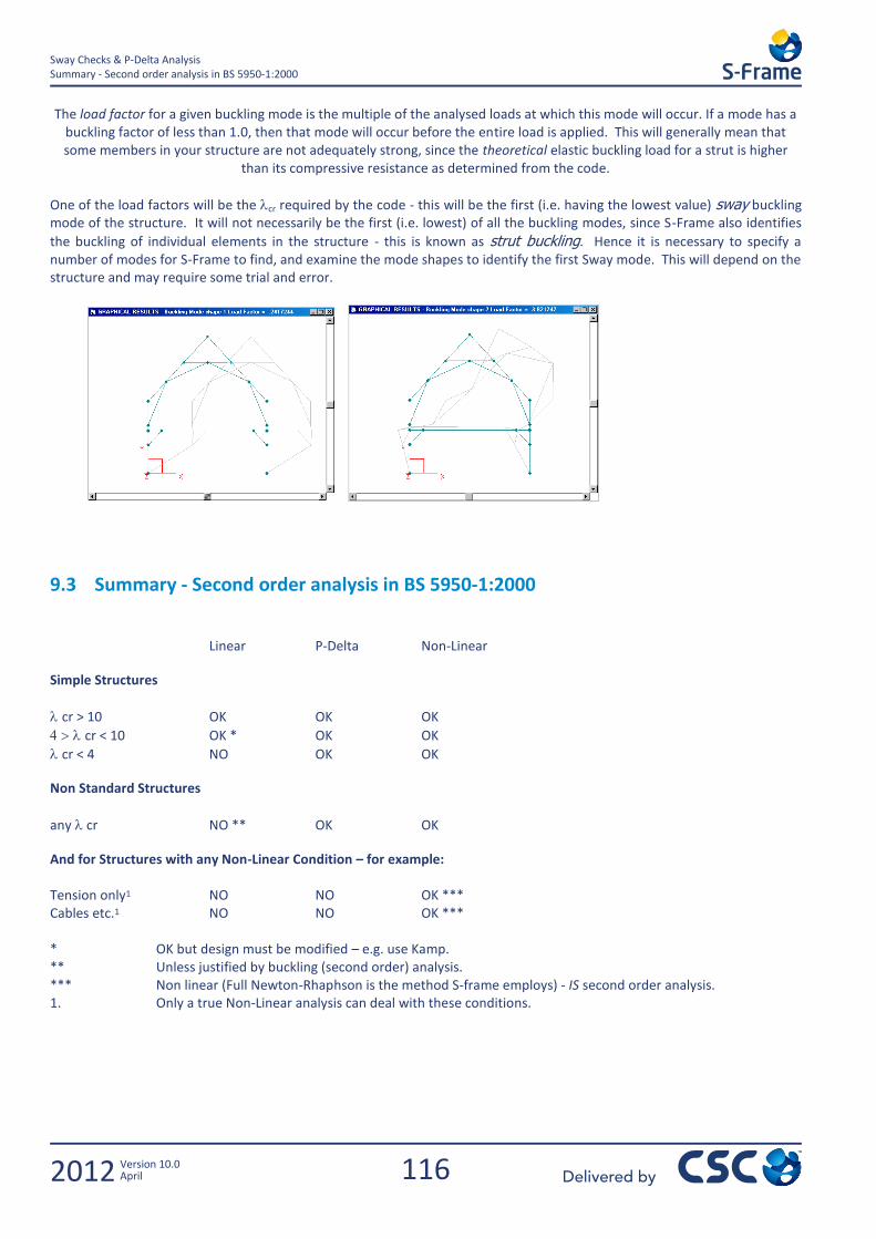
116
Sway Checks & P-Delta Analysis Summary - Second order analysis in BS 5950-1:2000
2012 Version 10.0 April
The load factor for a given buckling mode is the multiple of the analysed loads at which this mode will occur. If a mode has a buckling factor of less than 1.0, then that mode will occur before the entire load is applied. This will generally mean that some members in your structure are not adequately strong, since the theoretical elastic buckling load for a strut is higher
than its compressive resistance as determined from the code.
One of the load factors will be the cr required by the code - this will be the first (i.e. having the lowest value) sway buckling mode of the structure. It will not necessarily be the first (i.e. lowest) of all the buckling modes, since S-Frame also identifies
the buckling of individual elements in the structure - this is known as strut buckling. Hence it is necessary to specify a number of modes for S-Frame to find, and examine the mode shapes to identify the first Sway mode. This will depend on the structure and may require some trial and error.
9.3 Summary - Second order analysis in BS 5950-1:2000
Linear P-Delta Non-Linear
Simple Structures
cr > 10 OK OK OK
cr < 10 OK * OK OK
cr < 4 NO OK OK
Non Standard Structures
any cr NO ** OK OK
And for Structures with any Non-Linear Condition – for example: Tension only1 NO NO OK *** Cables etc.1 NO NO OK *** * OK but design must be modified – e.g. use Kamp. ** Unless justified by buckling (second order) analysis. *** Non linear (Full Newton-Rhaphson is the method S-frame employs) - IS second order analysis. 1. Only a true Non-Linear analysis can deal with these conditions.
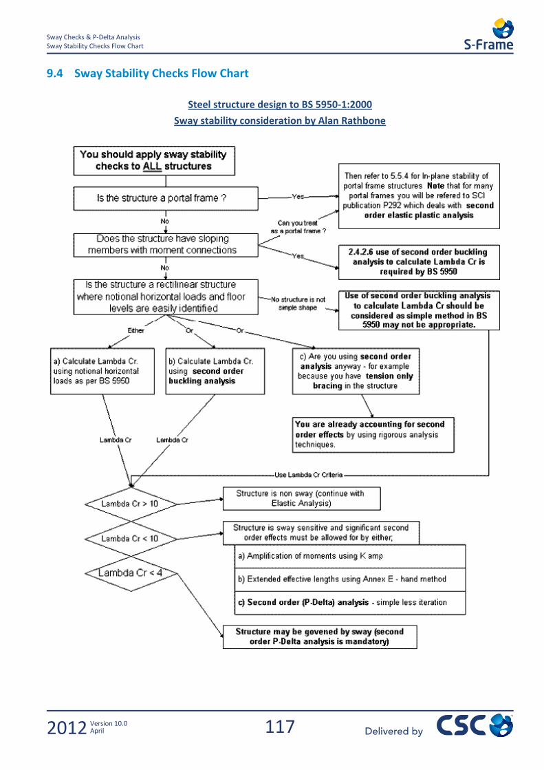
117
Sway Checks & P-Delta Analysis Sway Stability Checks Flow Chart
2012 Version 10.0 April
9.4 Sway Stability Checks Flow Chart
Steel structure design to BS 5950-1:2000
Sway stability consideration by Alan Rathbone


119
Sway Checks & P-Delta Analysis Sway Stability Checks Flow Chart
2012 Version 10.0 April
10.0 Sway Checks & P-Delta Analysis
Exercise

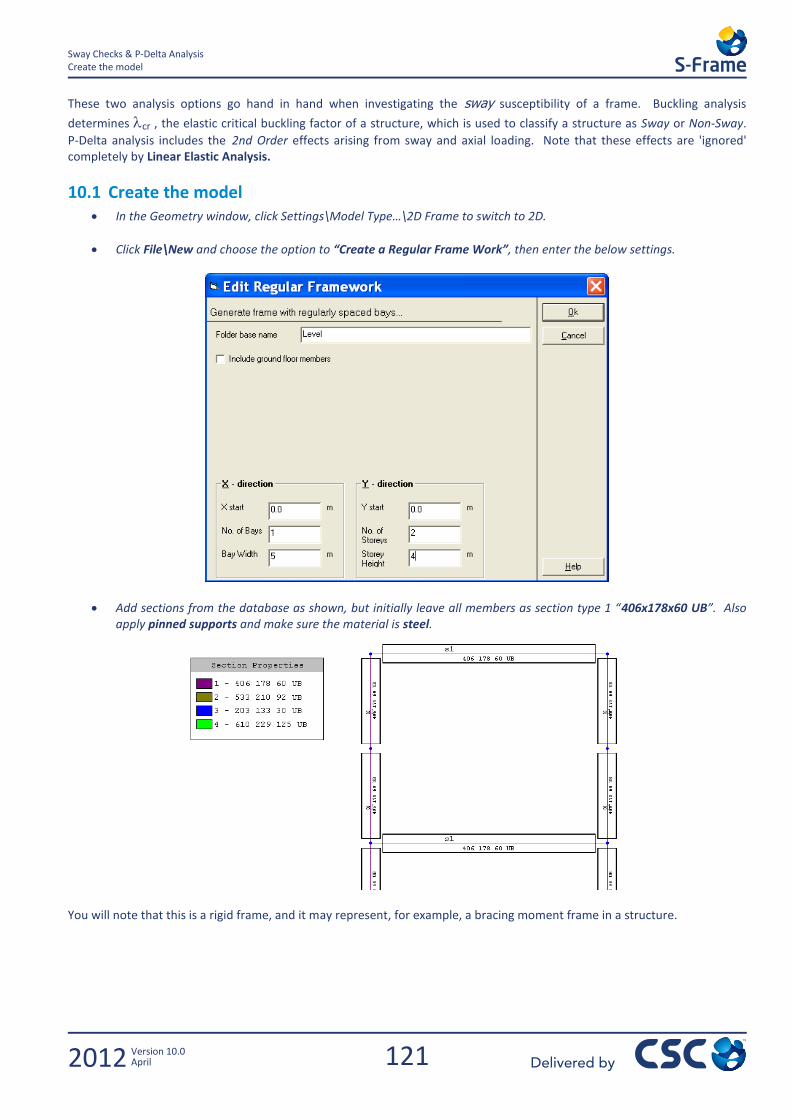
121
Sway Checks & P-Delta Analysis Create the model
2012 Version 10.0 April
These two analysis options go hand in hand when investigating the sway susceptibility of a frame. Buckling analysis
determines cr , the elastic critical buckling factor of a structure, which is used to classify a structure as Sway or Non-Sway.
P-Delta analysis includes the 2nd Order effects arising from sway and axial loading. Note that these effects are 'ignored' completely by Linear Elastic Analysis.
10.1 Create the model In the Geometry window, click Settings\Model Type…\2D Frame to switch to 2D.
Click File\New and choose the option to “Create a Regular Frame Work”, then enter the below settings.
Add sections from the database as shown, but initially leave all members as section type 1 “406x178x60 UB”. Also apply pinned supports and make sure the material is steel.
You will note that this is a rigid frame, and it may represent, for example, a bracing moment frame in a structure.
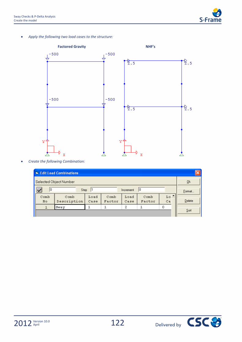
122
Sway Checks & P-Delta Analysis Create the model
2012 Version 10.0 April
Apply the following two load cases to the structure:
Factored Gravity NHF's
Create the following Combination:
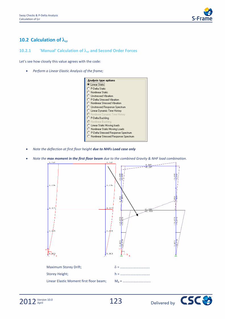
123
Sway Checks & P-Delta Analysis Calculation of (cr
2012 Version 10.0 April
10.2 Calculation of cr
10.2.1 'Manual' Calculation of cr and Second Order Forces
Let’s see how closely this value agrees with the code:
Perform a Linear Elastic Analysis of the frame;
Note the deflection at first floor height due to NHFs Load case only
Note the max moment in the first floor beam due to the combined Gravity & NHF load combination.
Maximum Storey Drift; = …………………………….
Storey Height; h = …………………………….
Linear Elastic Moment first floor beam; Me = …………………………..
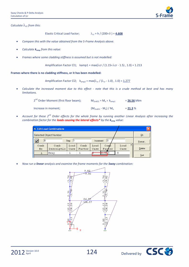
124
Sway Checks & P-Delta Analysis Calculation of (cr
2012 Version 10.0 April
Calculate cr from this:
Elastic Critical Load Factor; cr = h / (200 ) = 4.608
Compare this with the value obtained from the S-Frame Analysis above.
Calculate kamp from this value:
Frames where some cladding stiffness is assumed but is not modelled:
Amplification Factor Cl1; kamp1 = max(cr / (1.15cr - 1.5) , 1.0) = 1.213 Frames where there is no cladding stiffness, or it has been modelled:
Amplification Factor Cl2; kamp2 = max(cr / (cr - 1.0) , 1.0) = 1.277
Calculate the increased moment due to this effect - note that this is a crude method at best and has many limitations.
2nd
Order Moment (first floor beam); M2ndO1 = Me kamp1 = 26.56 kNm Increase in moment; (M2ndO1 - Me) / Me = 21.3 %
Account for these 2nd
Order effects for the whole frame by running another Linear Analysis after increasing the combination factor for the loads causing the lateral effects* by the kamp value:
Now run a linear analysis and examine the frame moments for the Sway combination:
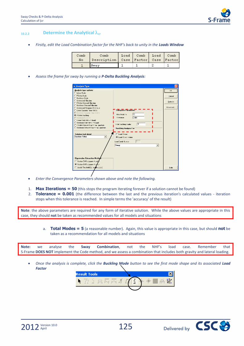
125
Sway Checks & P-Delta Analysis Calculation of (cr
2012 Version 10.0 April
10.2.2 Determine the Analytical cr
Firstly, edit the Load Combination factor for the NHF's back to unity in the Loads Window
Assess the frame for sway by running a P-Delta Buckling Analysis:
Enter the Convergence Parameters shown above and note the following.
1. Max Iterations = 50 (this stops the program iterating forever if a solution cannot be found)
2. Tolerance = 0.001 (the difference between the last and the previous iteration's calculated values - iteration stops when this tolerance is reached. In simple terms the 'accuracy' of the result)
Note: the above parameters are required for any form of iterative solution. While the above values are appropriate in this case, they should not be taken as recommended values for all models and situations
a. Total Modes = 5 (a reasonable number). Again, this value is appropriate in this case, but should not be taken as a recommendation for all models and situations
Note: we analyse the Sway Combination, not the NHF's load case. Remember that S-Frame DOES NOT implement the Code method, and we assess a combination that includes both gravity and lateral loading.
Once the analysis is complete, click the Buckling Mode button to see the first mode shape and its associated Load Factor
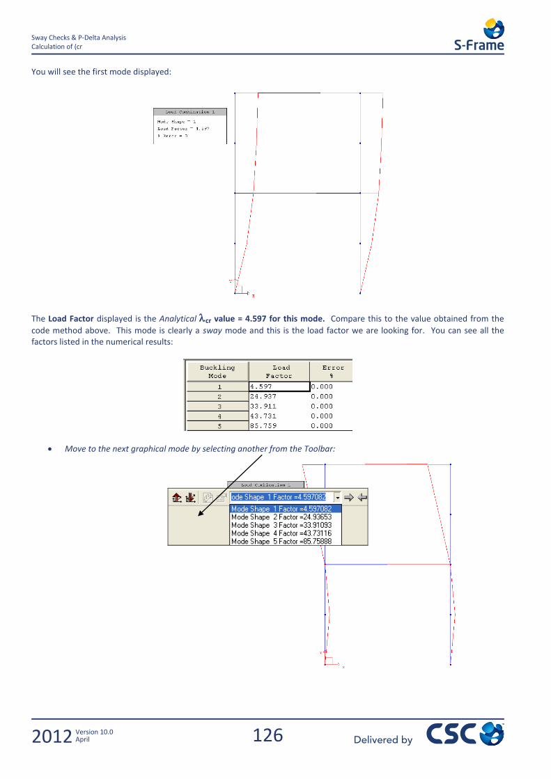
126
Sway Checks & P-Delta Analysis Calculation of (cr
2012 Version 10.0 April
You will see the first mode displayed:
The Load Factor displayed is the Analytical cr value = 4.597 for this mode. Compare this to the value obtained from the
code method above. This mode is clearly a sway mode and this is the load factor we are looking for. You can see all the factors listed in the numerical results:
Move to the next graphical mode by selecting another from the Toolbar:
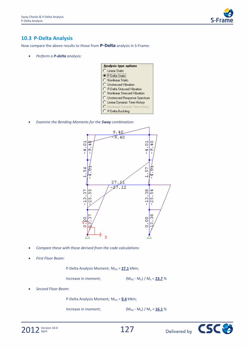
127
Sway Checks & P-Delta Analysis P-Delta Analysis
2012 Version 10.0 April
10.3 P-Delta Analysis Now compare the above results to those from P-Delta analysis in S-Frame:
Perform a P-delta analysis:
Examine the Bending Moments for the Sway combination:
Compare these with those derived from the code calculations:
First Floor Beam: P-Delta Analysis Moment; MPD = 27.1 kNm; Increase in moment; (MPD - Me) / Me = 23.7 %
Second Floor Beam:
P-Delta Analysis Moment; MPD = 9.4 kNm; Increase in moment; (MPD - Me) / Me = 16.1 %
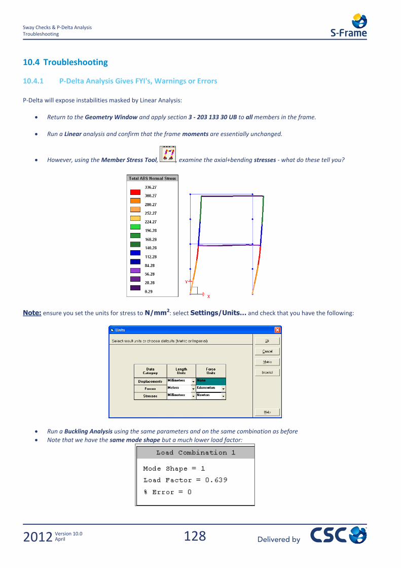
128
Sway Checks & P-Delta Analysis Troubleshooting
2012 Version 10.0 April
10.4 Troubleshooting
10.4.1 P-Delta Analysis Gives FYI's, Warnings or Errors
P-Delta will expose instabilities masked by Linear Analysis:
Return to the Geometry Window and apply section 3 - 203 133 30 UB to all members in the frame.
Run a Linear analysis and confirm that the frame moments are essentially unchanged.
However, using the Member Stress Tool, , examine the axial+bending stresses - what do these tell you?
Note: ensure you set the units for stress to N/mm2: select Settings/Units… and check that you have the following:
Run a Buckling Analysis using the same parameters and on the same combination as before
Note that we have the same mode shape but a much lower load factor:
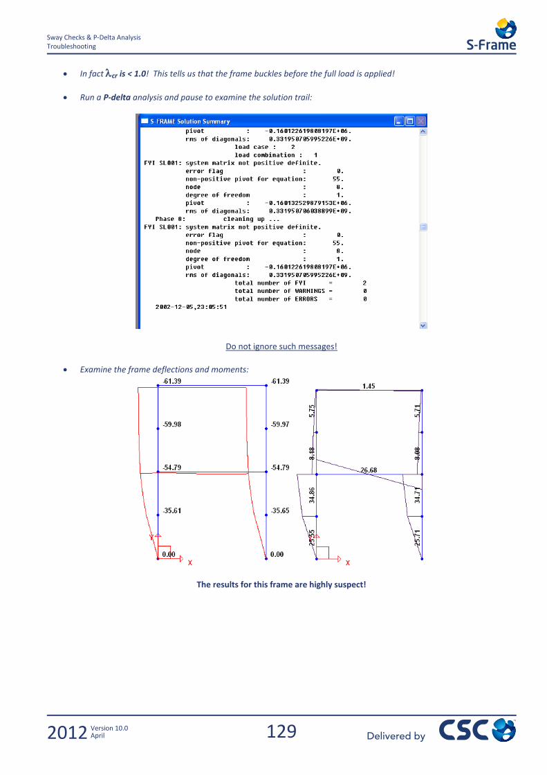
129
Sway Checks & P-Delta Analysis Troubleshooting
2012 Version 10.0 April
In fact cr is < 1.0! This tells us that the frame buckles before the full load is applied!
Run a P-delta analysis and pause to examine the solution trail:
Do not ignore such messages!
Examine the frame deflections and moments:
The results for this frame are highly suspect!
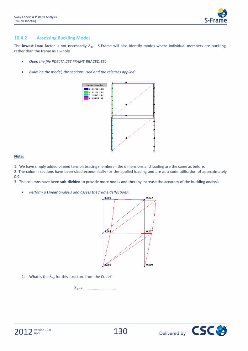
130
Sway Checks & P-Delta Analysis Troubleshooting
2012 Version 10.0 April
10.4.2 Assessing Buckling Modes
The lowest Load factor is not necessarily cr. S-Frame will also identify modes where individual members are buckling,
rather than the frame as a whole.
Open the file PDELTA 2ST FRAME BRACED.TEL
Examine the model, the sections used and the releases applied:
Note: 1. We have simply added pinned tension bracing members - the dimensions and loading are the same as before. 2. The column sections have been sized economically for the applied loading and are at a code utilisation of approximately 0.9. 3. The columns have been sub-divided to provide more nodes and thereby increase the accuracy of the buckling analysis
Perform a Linear analysis and assess the frame deflections:
1. What is the cr for this structure from the Code?
cr = …………………………….
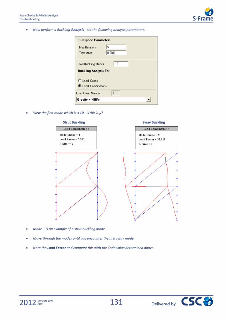
131
Sway Checks & P-Delta Analysis Troubleshooting
2012 Version 10.0 April
Now perform a Buckling Analysis - set the following analysis parameters:
View the first mode which is < 10 - is this cr?
Strut Buckling Sway Buckling
Mode 1 is an example of a strut buckling mode.
Move through the modes until you encounter the first sway mode.
Note the Load Factor and compare this with the Code value determined above.

132
Sway Checks & P-Delta Analysis Further Investigation
2012 Version 10.0 April
10.5 Further Investigation
What if cr > 10? The code says you can ignore 2nd
order effects, but do they occur?
What is the cr value for the frame if you use section 2 - 533 210 92 UB?
cr = ……………………………..?
kamp = …………………………….?
Run a P-delta analysis - what is the moment in the first floor beam?
M2ndO = ………………………………? % increase = …………………………?

133
S-Steel Design Further Investigation
2012 Version 10.0 April
11.0 S-Steel Design

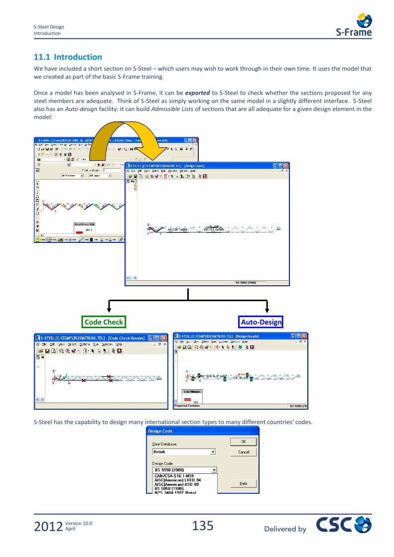
135
S-Steel Design Introduction
2012 Version 10.0 April
11.1 Introduction We have included a short section on S-Steel – which users may wish to work through in their own time. It uses the model that we created as part of the basic S-Frame training. Once a model has been analysed in S-Frame, it can be exported to S-Steel to check whether the sections proposed for any steel members are adequate. Think of S-Steel as simply working on the same model in a slightly different interface. S-Steel also has an Auto-design facility: it can build Admissible Lists of sections that are all adequate for a given design element in the model:
Code Check Auto-Design
S-Steel has the capability to design many international section types to many different countries' codes.
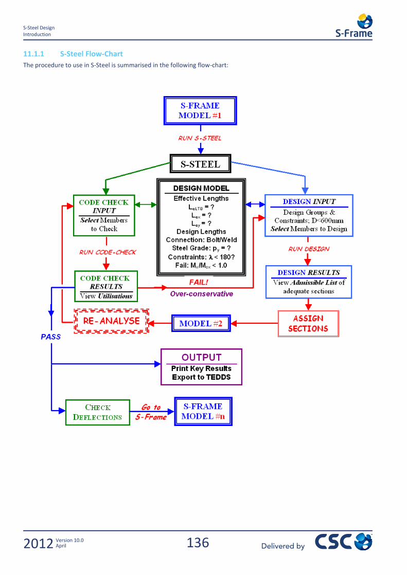
136
S-Steel Design Introduction
2012 Version 10.0 April
11.1.1 S-Steel Flow-Chart
The procedure to use in S-Steel is summarised in the following flow-chart:
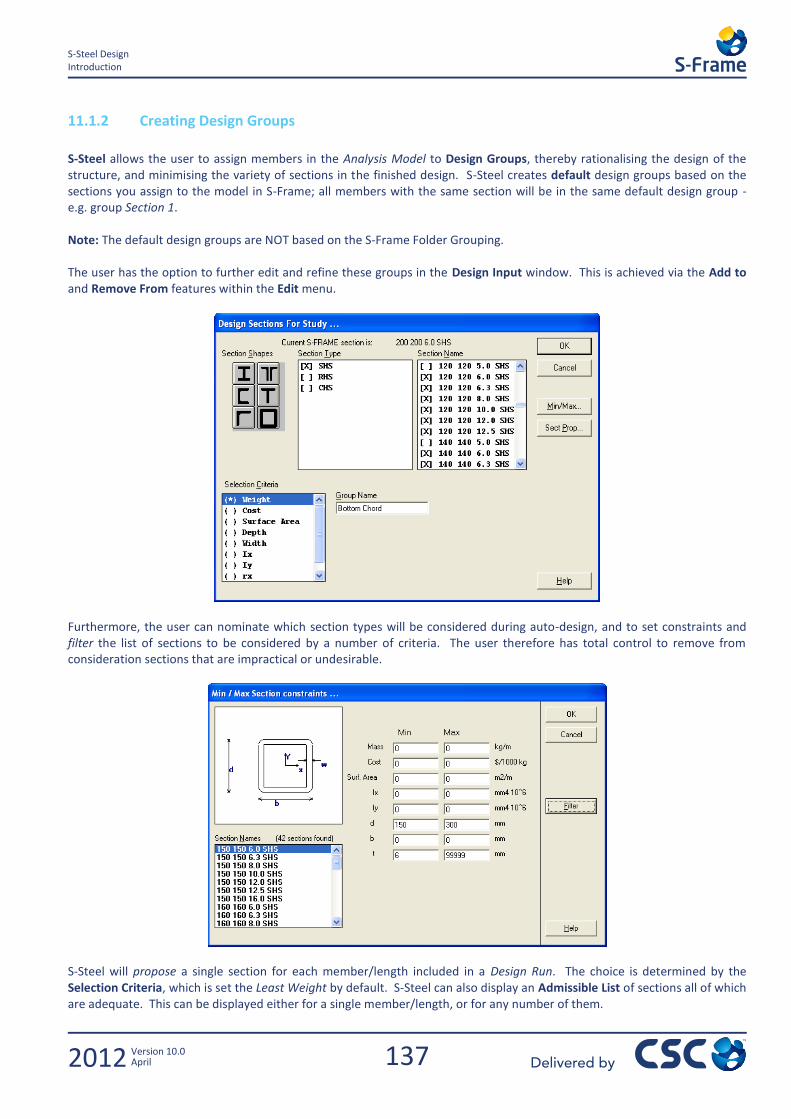
137
S-Steel Design Introduction
2012 Version 10.0 April
11.1.2 Creating Design Groups
S-Steel allows the user to assign members in the Analysis Model to Design Groups, thereby rationalising the design of the structure, and minimising the variety of sections in the finished design. S-Steel creates default design groups based on the sections you assign to the model in S-Frame; all members with the same section will be in the same default design group - e.g. group Section 1. Note: The default design groups are NOT based on the S-Frame Folder Grouping. The user has the option to further edit and refine these groups in the Design Input window. This is achieved via the Add to and Remove From features within the Edit menu.
Furthermore, the user can nominate which section types will be considered during auto-design, and to set constraints and filter the list of sections to be considered by a number of criteria. The user therefore has total control to remove from consideration sections that are impractical or undesirable.
S-Steel will propose a single section for each member/length included in a Design Run. The choice is determined by the Selection Criteria, which is set the Least Weight by default. S-Steel can also display an Admissible List of sections all of which are adequate. This can be displayed either for a single member/length, or for any number of them.
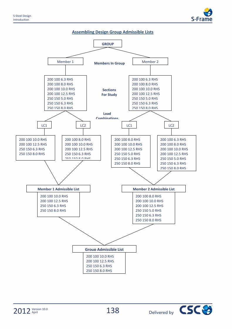
138
S-Steel Design Introduction
2012 Version 10.0 April
Assembling Design Group Admissible Lists
Members In Group
Sections For Study
LC1
200 100 10.0 RHS 200 100 12.5 RHS 250 150 6.3 RHS 250 150 8.0 RHS
200 100 6.3 RHS 200 100 8.0 RHS 200 100 10.0 RHS 200 100 12.5 RHS 250 150 5.0 RHS 250 150 6.3 RHS 250 150 8.0 RHS
GROUP
Member 1
LC1 LC2 LC2
200 100 6.3 RHS 200 100 8.0 RHS 200 100 10.0 RHS 200 100 12.5 RHS 250 150 5.0 RHS 250 150 6.3 RHS 250 150 8.0 RHS
200 100 6.3 RHS 200 100 8.0 RHS 200 100 10.0 RHS 200 100 12.5 RHS 250 150 5.0 RHS 250 150 6.3 RHS 250 150 8.0 RHS
200 100 8.0 RHS 200 100 10.0 RHS 200 100 12.5 RHS 250 150 6.3 RHS 250 150 8.0 RHS
200 100 8.0 RHS 200 100 10.0 RHS 200 100 12.5 RHS 250 150 5.0 RHS 250 150 6.3 RHS 250 150 8.0 RHS
Member 1 Admissible List Member 2 Admissible List
200 100 10.0 RHS 200 100 12.5 RHS 250 150 6.3 RHS 250 150 8.0 RHS
200 100 8.0 RHS 200 100 10.0 RHS 200 100 12.5 RHS 250 150 5.0 RHS 250 150 6.3 RHS 250 150 8.0 RHS
200 100 10.0 RHS 200 100 12.5 RHS 250 150 6.3 RHS 250 150 8.0 RHS
Group Admissible List
Member 2
Load Combinations

139
S-Steel Design Introduction
2012 Version 10.0 April
11.1.3 The "Design Model" & Performing a Code Check
First you should consider the Design Model of design information - all the following have assumed values which may or may not be correct for your structure.
Design Lengths; Make Continuous Effective Lengths; Lex , Ley , LeLTB Connection Type; Bolted/Welded Steel Grade; py = ? Constraints Neglected Force Limits
Slenderness Limits; Compression and Tension < ? Failure Limit (Code Relaxation); Mx/Mcx < ?
Make Continuous Select members - note that these must be adjacent and co-linear- then Edit/ Make Continuous.
Effective Lengths Select member(s), then Edit/ Effective Lengths The Top and Bottom Flange effective lengths set LeLTB - note that these are ignored for Structural Hollow Sections where LeLTB = 0.
Connection Type
Select member(s), then Edit/ Connection Type…
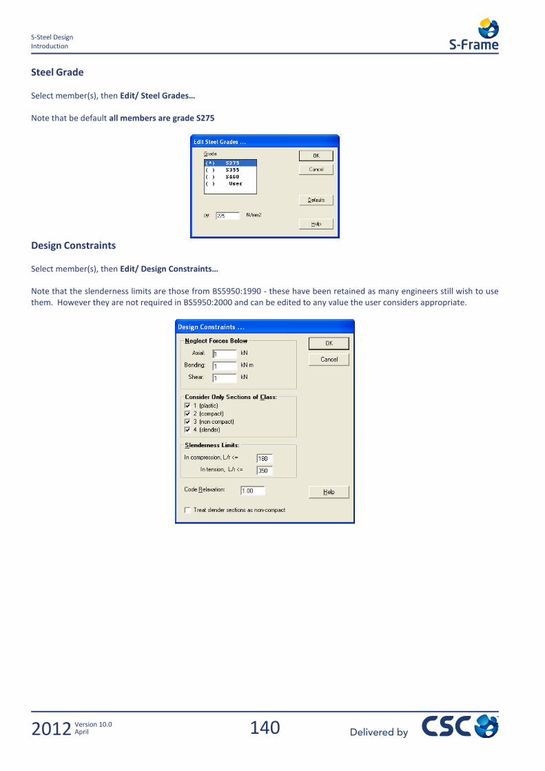
140
S-Steel Design Introduction
2012 Version 10.0 April
Steel Grade Select member(s), then Edit/ Steel Grades… Note that be default all members are grade S275
Design Constraints Select member(s), then Edit/ Design Constraints… Note that the slenderness limits are those from BS5950:1990 - these have been retained as many engineers still wish to use them. However they are not required in BS5950:2000 and can be edited to any value the user considers appropriate.
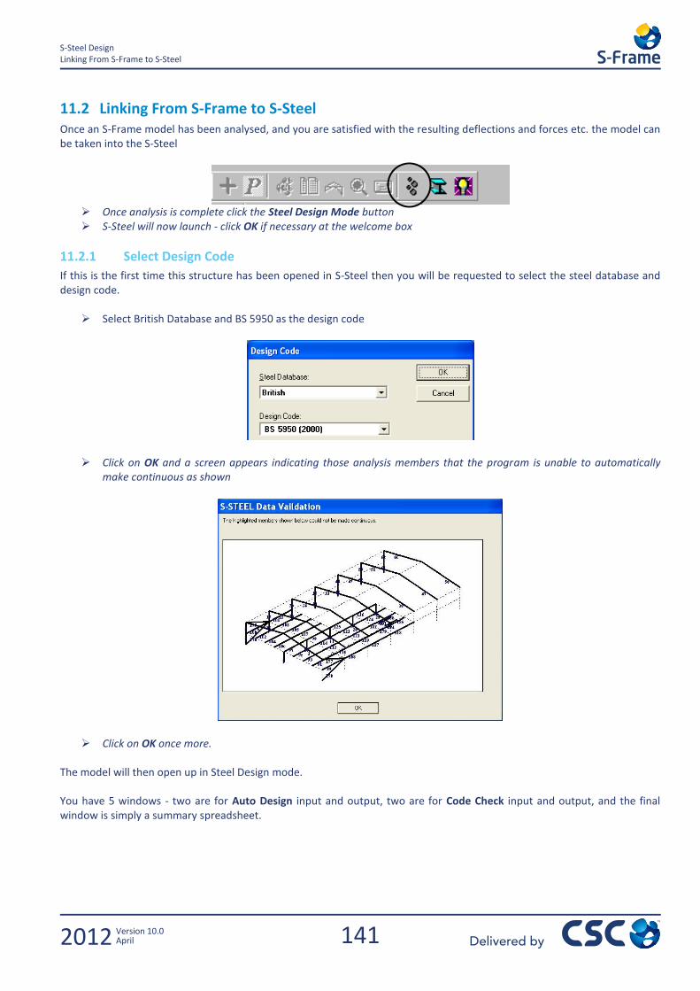
141
S-Steel Design Linking From S-Frame to S-Steel
2012 Version 10.0 April
11.2 Linking From S-Frame to S-Steel Once an S-Frame model has been analysed, and you are satisfied with the resulting deflections and forces etc. the model can be taken into the S-Steel
Once analysis is complete click the Steel Design Mode button S-Steel will now launch - click OK if necessary at the welcome box
11.2.1 Select Design Code
If this is the first time this structure has been opened in S-Steel then you will be requested to select the steel database and design code.
Select British Database and BS 5950 as the design code
Click on OK and a screen appears indicating those analysis members that the program is unable to automatically make continuous as shown
Click on OK once more.
The model will then open up in Steel Design mode. You have 5 windows - two are for Auto Design input and output, two are for Code Check input and output, and the final window is simply a summary spreadsheet.
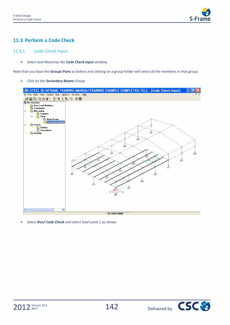
142
S-Steel Design Perform a Code Check
2012 Version 10.0 April
11.3 Perform a Code Check
11.3.1 Code Check Input
Select and Maximise the Code Check Input window.
Note that you have the Groups Pane as before and clicking on a group folder will select all the members in that group.
Click on the Secondary Beams Group.
Select Run/ Code Check and select load comb 1 as shown
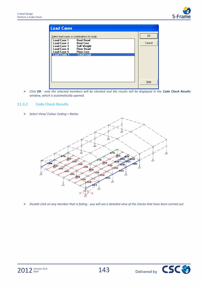
143
S-Steel Design Perform a Code Check
2012 Version 10.0 April
Click OK - only the selected members will be checked and the results will be displayed in the Code Check Results
window, which is automatically opened.
11.3.2 Code Check Results
Select View/ Colour Coding + Ratios
Double-click on any member that is failing - you will see a detailed view of the checks that have been carried out:
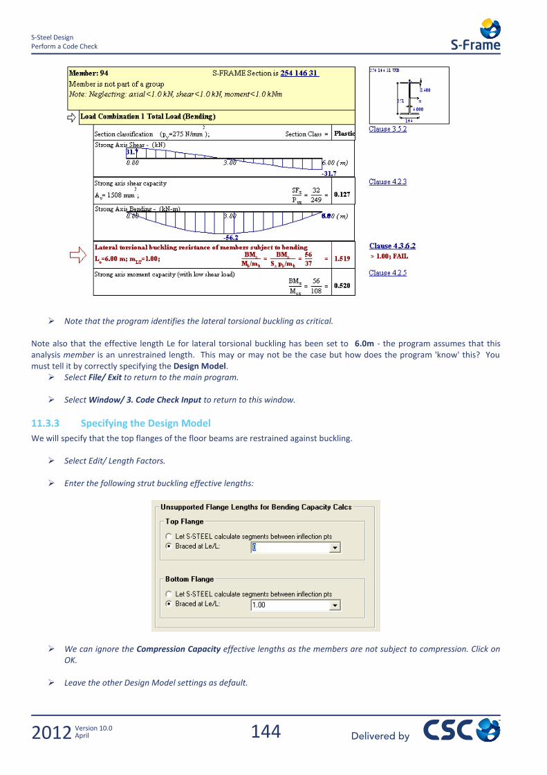
144
S-Steel Design Perform a Code Check
2012 Version 10.0 April
Note that the program identifies the lateral torsional buckling as critical.
Note also that the effective length Le for lateral torsional buckling has been set to 6.0m - the program assumes that this analysis member is an unrestrained length. This may or may not be the case but how does the program 'know' this? You must tell it by correctly specifying the Design Model.
Select File/ Exit to return to the main program.
Select Window/ 3. Code Check Input to return to this window.
11.3.3 Specifying the Design Model
We will specify that the top flanges of the floor beams are restrained against buckling.
Select Edit/ Length Factors.
Enter the following strut buckling effective lengths:
We can ignore the Compression Capacity effective lengths as the members are not subject to compression. Click on OK.
Leave the other Design Model settings as default.
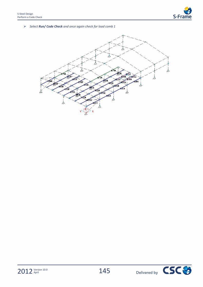
145
S-Steel Design Perform a Code Check
2012 Version 10.0 April
Select Run/ Code Check and once again check for load comb 1
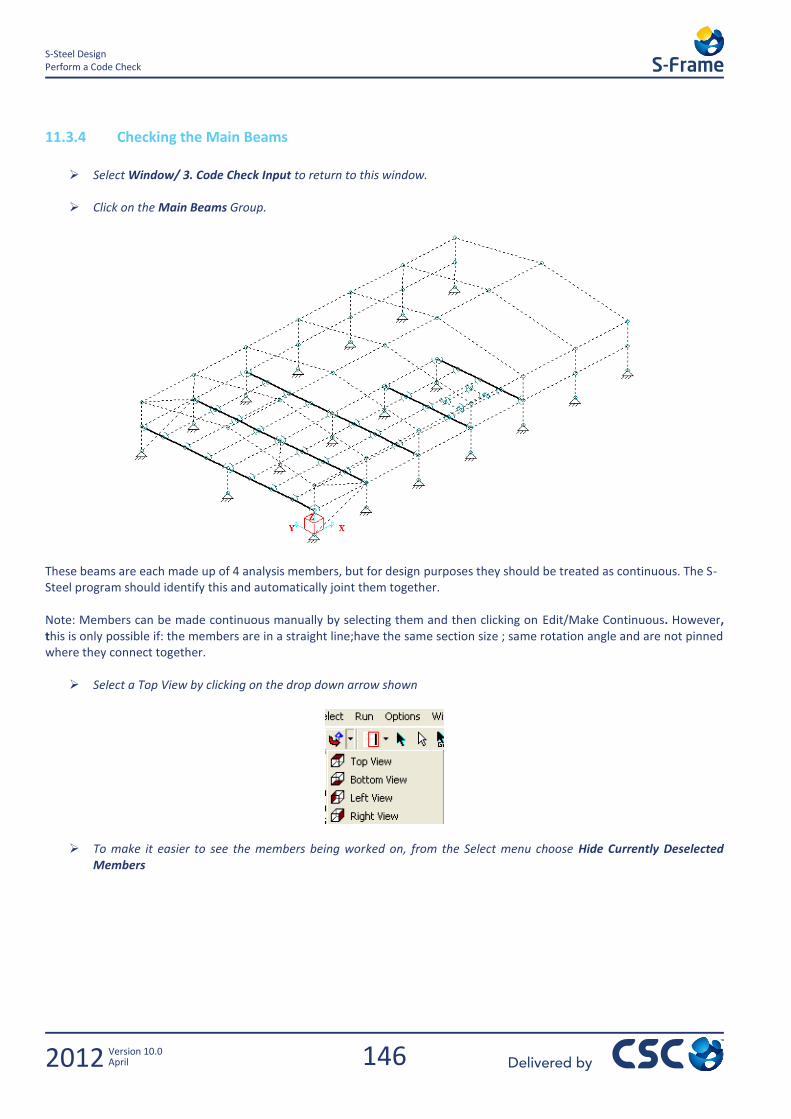
146
S-Steel Design Perform a Code Check
2012 Version 10.0 April
11.3.4 Checking the Main Beams
Select Window/ 3. Code Check Input to return to this window.
Click on the Main Beams Group.
These beams are each made up of 4 analysis members, but for design purposes they should be treated as continuous. The S-Steel program should identify this and automatically joint them together. Note: Members can be made continuous manually by selecting them and then clicking on Edit/Make Continuous. However, this is only possible if: the members are in a straight line;have the same section size ; same rotation angle and are not pinned where they connect together.
Select a Top View by clicking on the drop down arrow shown
To make it easier to see the members being worked on, from the Select menu choose Hide Currently Deselected Members
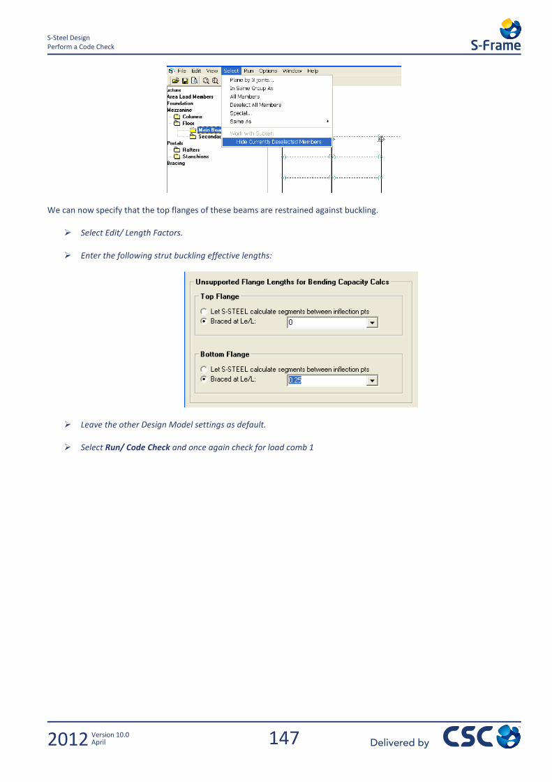
147
S-Steel Design Perform a Code Check
2012 Version 10.0 April
We can now specify that the top flanges of these beams are restrained against buckling.
Select Edit/ Length Factors.
Enter the following strut buckling effective lengths:
Leave the other Design Model settings as default.
Select Run/ Code Check and once again check for load comb 1
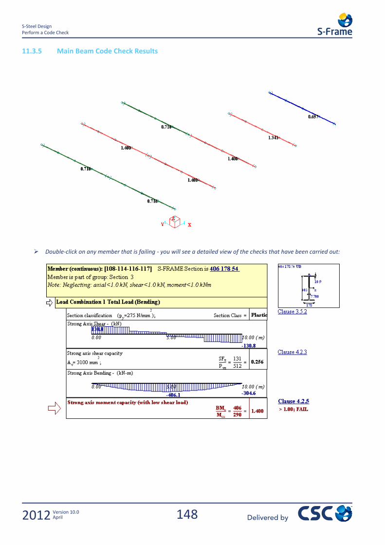
148
S-Steel Design Perform a Code Check
2012 Version 10.0 April
11.3.5 Main Beam Code Check Results
Double-click on any member that is failing - you will see a detailed view of the checks that have been carried out:
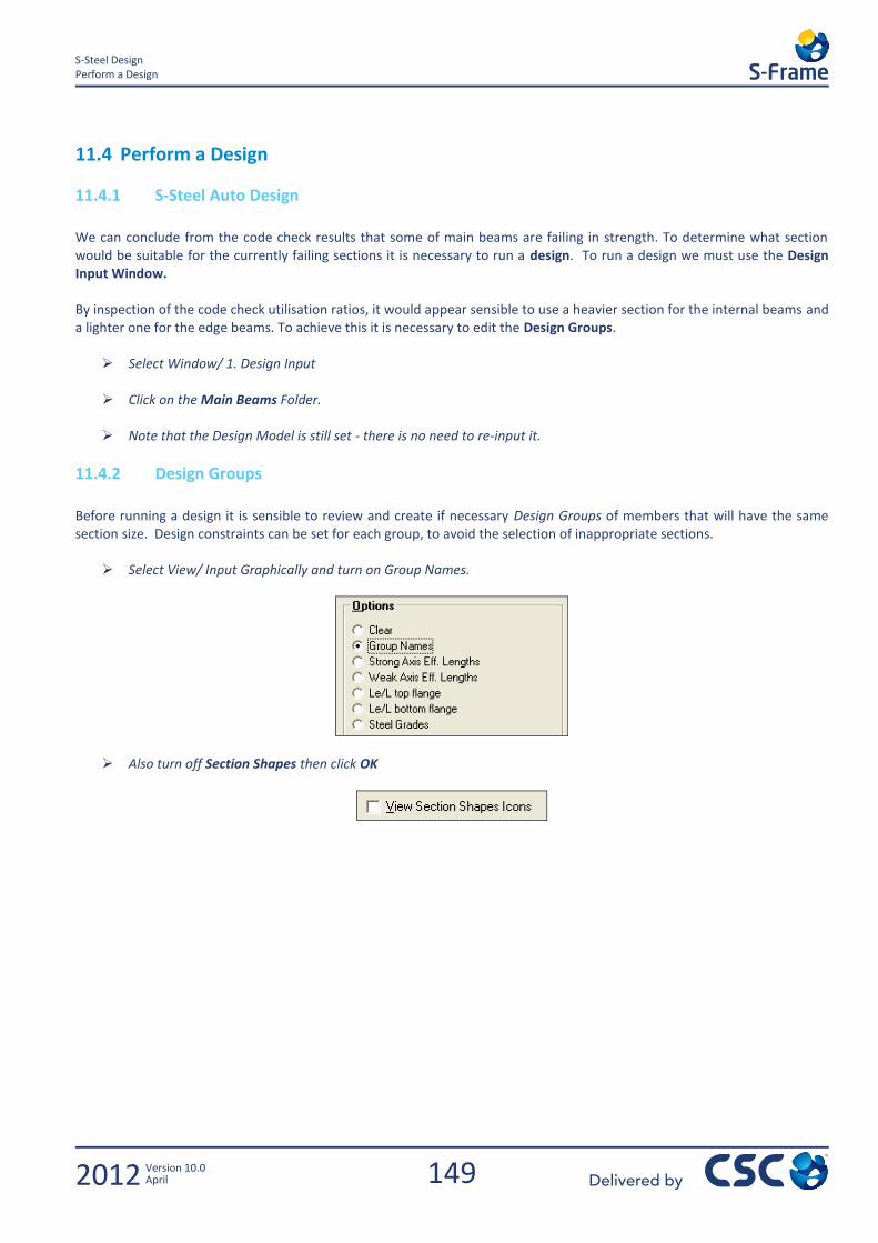
149
S-Steel Design Perform a Design
2012 Version 10.0 April
11.4 Perform a Design
11.4.1 S-Steel Auto Design
We can conclude from the code check results that some of main beams are failing in strength. To determine what section would be suitable for the currently failing sections it is necessary to run a design. To run a design we must use the Design Input Window. By inspection of the code check utilisation ratios, it would appear sensible to use a heavier section for the internal beams and a lighter one for the edge beams. To achieve this it is necessary to edit the Design Groups.
Select Window/ 1. Design Input
Click on the Main Beams Folder.
Note that the Design Model is still set - there is no need to re-input it.
11.4.2 Design Groups
Before running a design it is sensible to review and create if necessary Design Groups of members that will have the same section size. Design constraints can be set for each group, to avoid the selection of inappropriate sections.
Select View/ Input Graphically and turn on Group Names.
Also turn off Section Shapes then click OK
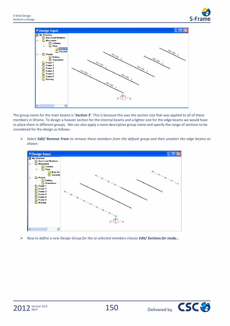
150
S-Steel Design Perform a Design
2012 Version 10.0 April
The group name for the main beams is ‘Section 3’. This is because this was the section size that was applied to all of these members in Sframe. To design a heavier section for the internal beams and a lighter one for the edge beams we would have to place them in different groups. We can also apply a more descriptive group name and specify the range of sections to be considered for the design as follows:
Select Edit/ Remove From to remove these members from the default group and then unselect the edge beams as shown:
Now to define a new Design Group for the se selected members choose Edit/ Sections for study…
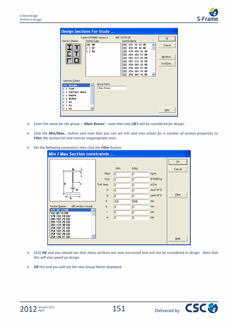
151
S-Steel Design Perform a Design
2012 Version 10.0 April
Enter the name for the group – ‘Main Beams’ - note that only UB's will be considered for design.
Click the Min/Max… button and note that you can set min and max values for a number of section properties to Filter the section list and remove inappropriate ones.
Set the following constraints then click the Filter button:
Click OK and you should see that many sections are now uncrossed and will not be considered in design. Note that this will also speed up design.
OK this and you will see the new Group Name displayed.
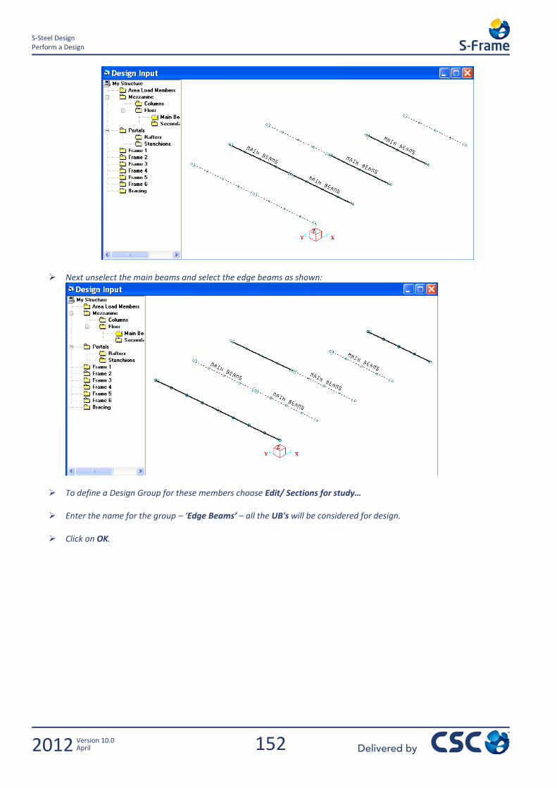
152
S-Steel Design Perform a Design
2012 Version 10.0 April
Next unselect the main beams and select the edge beams as shown:
To define a Design Group for these members choose Edit/ Sections for study…
Enter the name for the group – ‘Edge Beams’ – all the UB's will be considered for design.
Click on OK.
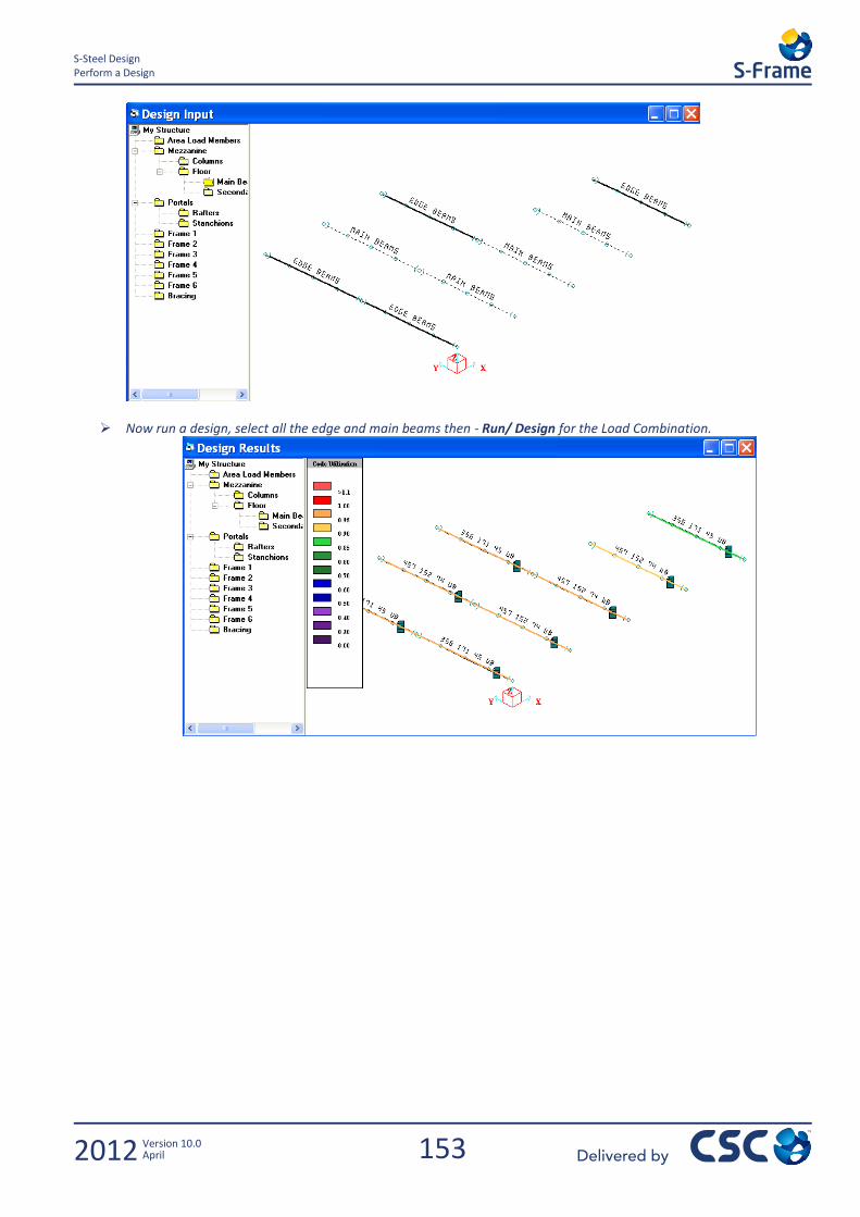
153
S-Steel Design Perform a Design
2012 Version 10.0 April
Now run a design, select all the edge and main beams then - Run/ Design for the Load Combination.
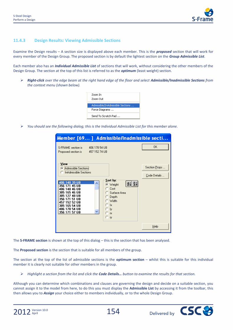
154
S-Steel Design Perform a Design
2012 Version 10.0 April
11.4.3 Design Results: Viewing Admissible Sections
Examine the Design results – A section size is displayed above each member. This is the proposed section that will work for every member of the Design Group. The proposed section is by default the lightest section on the Group Admissible List. Each member also has an Individual Admissible List of sections that will work, without considering the other members of the Design Group. The section at the top of this list is referred to as the optimum (least weight) section.
Right-click over the edge beam at the right hand edge of the floor and select Admissible/Inadmissible Sections from the context menu (shown below).
You should see the following dialog; this is the Individual Admissible List for this member alone.
The S-FRAME section is shown at the top of this dialog – this is the section that has been analysed. The Proposed section is the section that is suitable for all members of the group. The section at the top of the list of admissible sections is the optimum section – whilst this is suitable for this individual member it is clearly not suitable for other members in the group.
Highlight a section from the list and click the Code Details… button to examine the results for that section.
Although you can determine which combinations and clauses are governing the design and decide on a suitable section, you cannot assign it to the model from here, to do this you must display the Admissible List by accessing it from the toolbar, this then allows you to Assign your choice either to members individually, or to the whole Design Group.
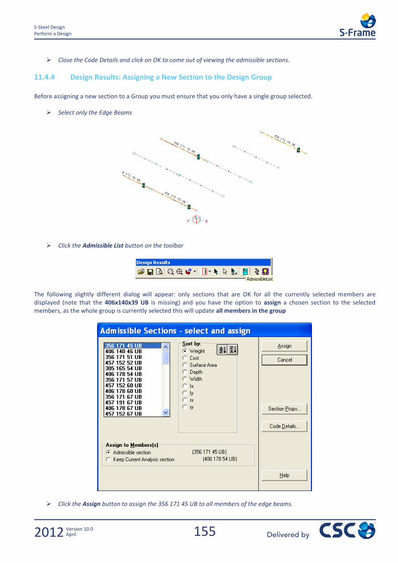
155
S-Steel Design Perform a Design
2012 Version 10.0 April
Close the Code Details and click on OK to come out of viewing the admissible sections.
11.4.4 Design Results: Assigning a New Section to the Design Group
Before assigning a new section to a Group you must ensure that you only have a single group selected.
Select only the Edge Beams
Click the Admissible List button on the toolbar
The following slightly different dialog will appear: only sections that are OK for all the currently selected members are displayed (note that the 406x140x39 UB is missing) and you have the option to assign a chosen section to the selected members, as the whole group is currently selected this will update all members in the group
Click the Assign button to assign the 356 171 45 UB to all members of the edge beams.
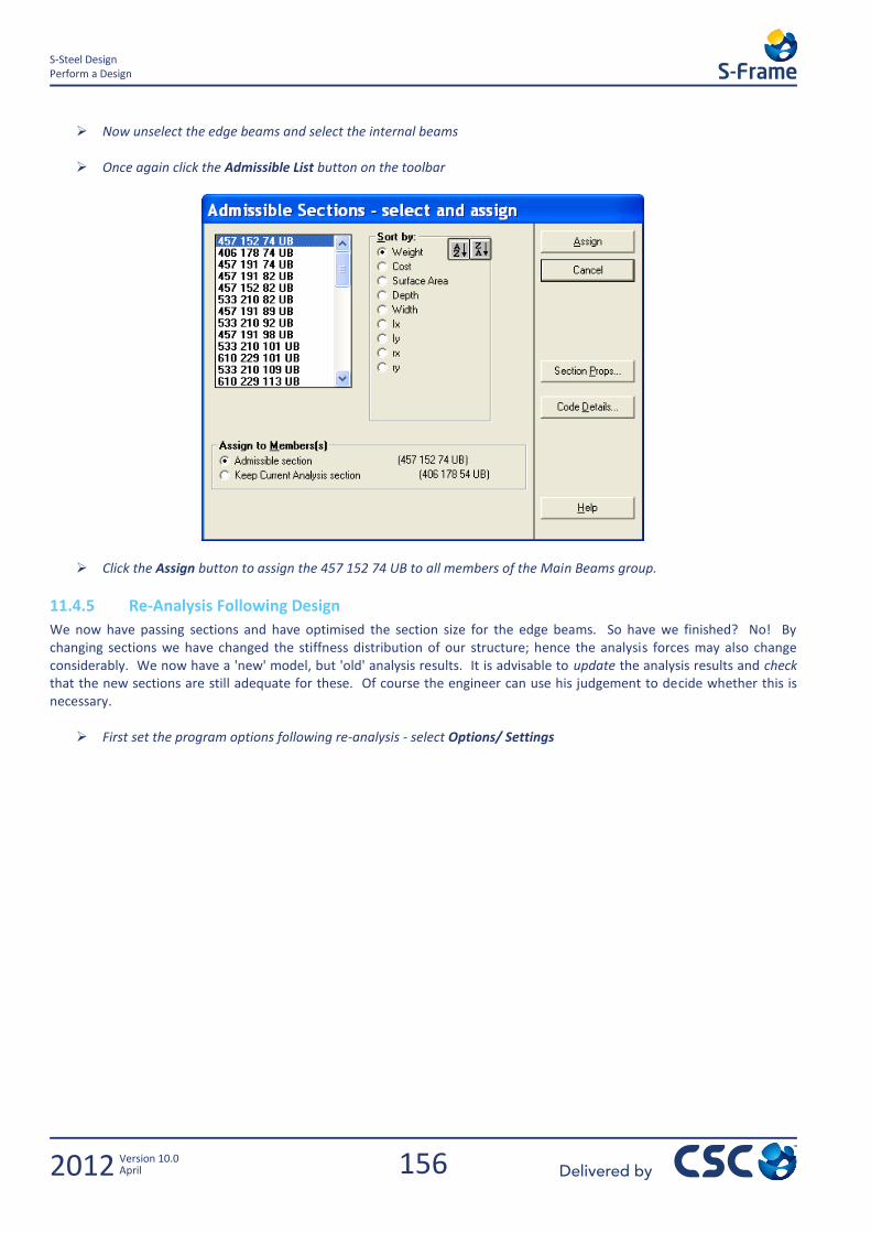
156
S-Steel Design Perform a Design
2012 Version 10.0 April
Now unselect the edge beams and select the internal beams
Once again click the Admissible List button on the toolbar
Click the Assign button to assign the 457 152 74 UB to all members of the Main Beams group.
11.4.5 Re-Analysis Following Design
We now have passing sections and have optimised the section size for the edge beams. So have we finished? No! By changing sections we have changed the stiffness distribution of our structure; hence the analysis forces may also change considerably. We now have a 'new' model, but 'old' analysis results. It is advisable to update the analysis results and check that the new sections are still adequate for these. Of course the engineer can use his judgement to decide whether this is necessary.
First set the program options following re-analysis - select Options/ Settings
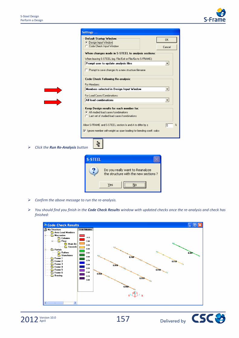
157
S-Steel Design Perform a Design
2012 Version 10.0 April
Click the Run Re-Analysis button
Confirm the above message to run the re-analysis. You should find you finish in the Code Check Results window with updated checks once the re-analysis and check has
finished:

158
S-Steel Design Perform a Design
2012 Version 10.0 April
Note: Re-analysis of the new (heavier) sections will have increased the design forces in the members. However, in this case the change is insufficient to cause any members to fail. If a failure had occurred a further design/re-analysis pass would be required.
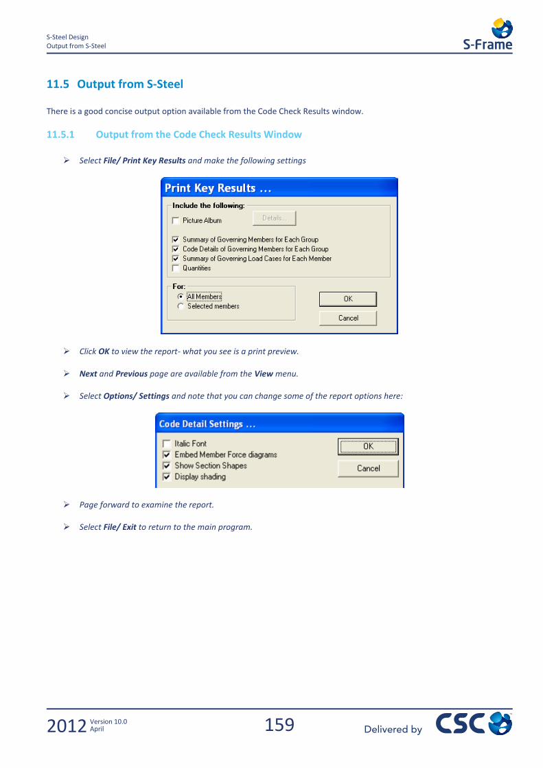
159
S-Steel Design Output from S-Steel
2012 Version 10.0 April
11.5 Output from S-Steel There is a good concise output option available from the Code Check Results window.
11.5.1 Output from the Code Check Results Window
Select File/ Print Key Results and make the following settings
Click OK to view the report- what you see is a print preview.
Next and Previous page are available from the View menu.
Select Options/ Settings and note that you can change some of the report options here:
Page forward to examine the report.
Select File/ Exit to return to the main program.
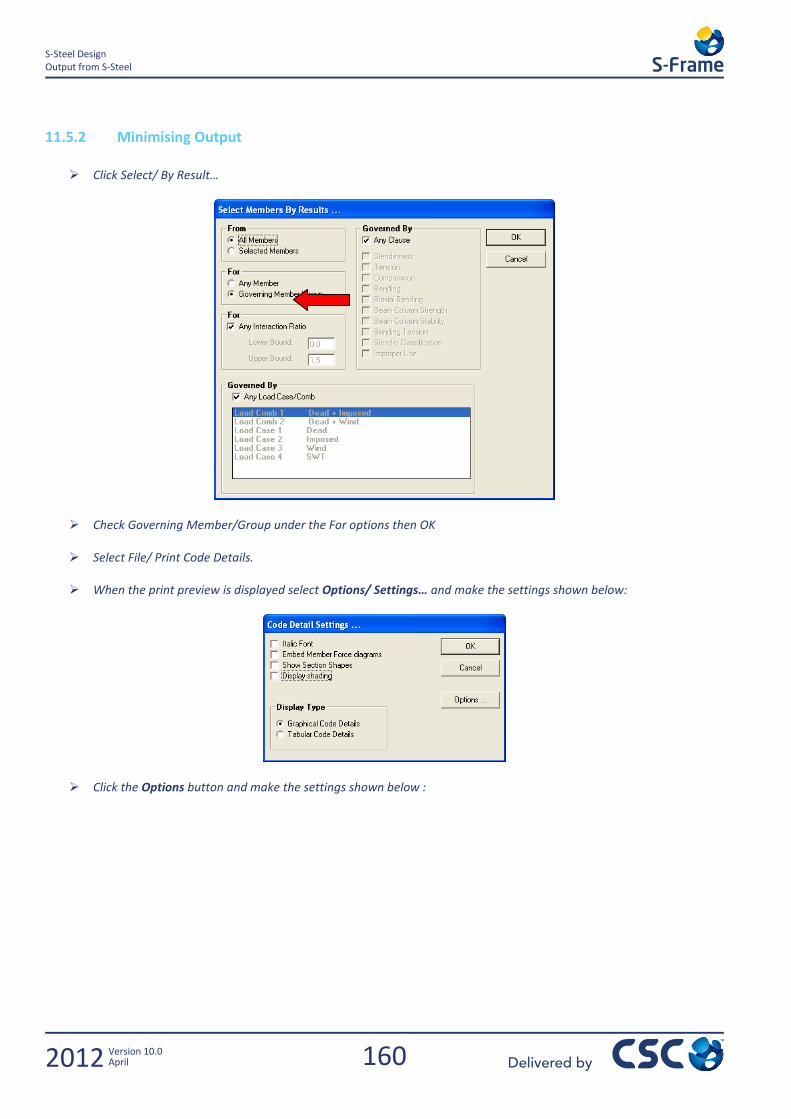
160
S-Steel Design Output from S-Steel
2012 Version 10.0 April
11.5.2 Minimising Output
Click Select/ By Result…
Check Governing Member/Group under the For options then OK
Select File/ Print Code Details.
When the print preview is displayed select Options/ Settings… and make the settings shown below:
Click the Options button and make the settings shown below :
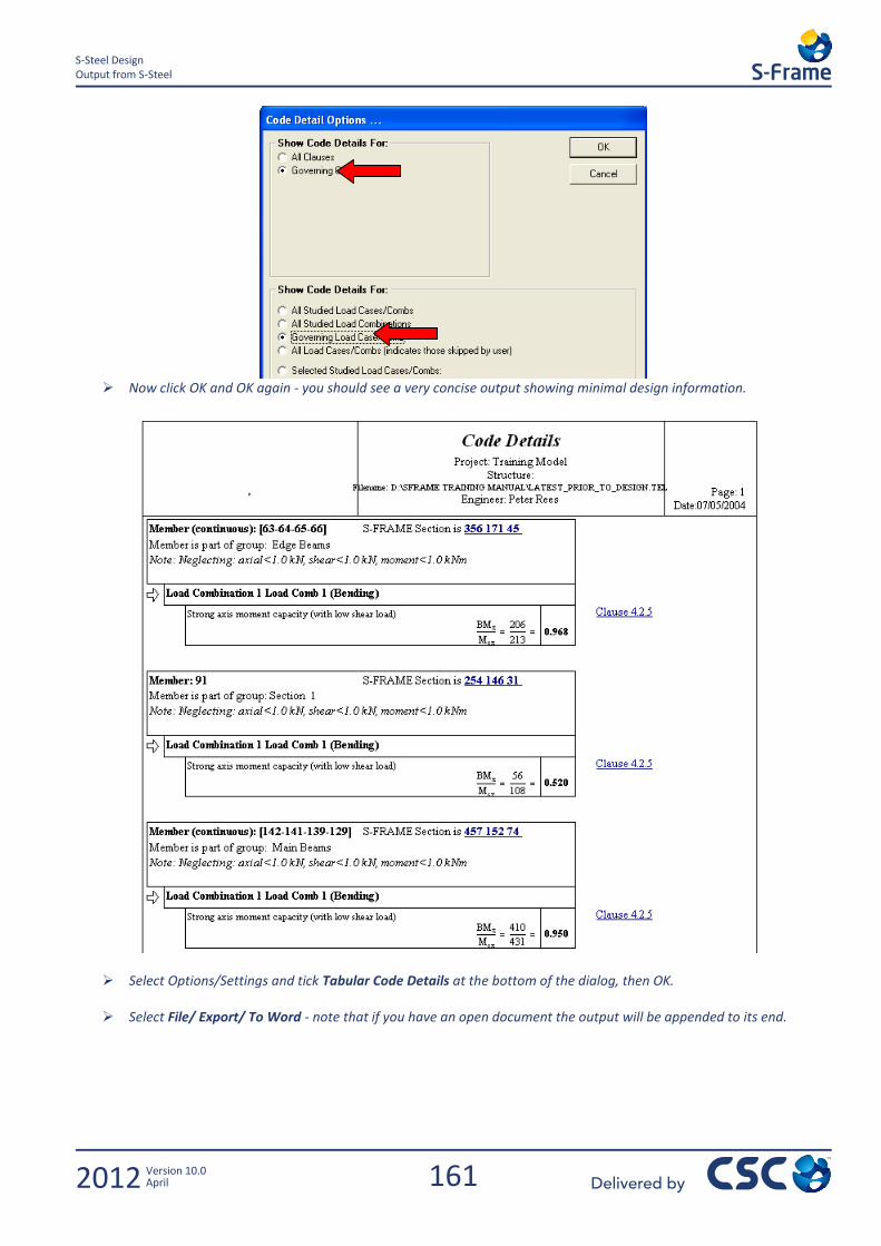
161
S-Steel Design Output from S-Steel
2012 Version 10.0 April
Now click OK and OK again - you should see a very concise output showing minimal design information.
Select Options/Settings and tick Tabular Code Details at the bottom of the dialog, then OK.
Select File/ Export/ To Word - note that if you have an open document the output will be appended to its end.
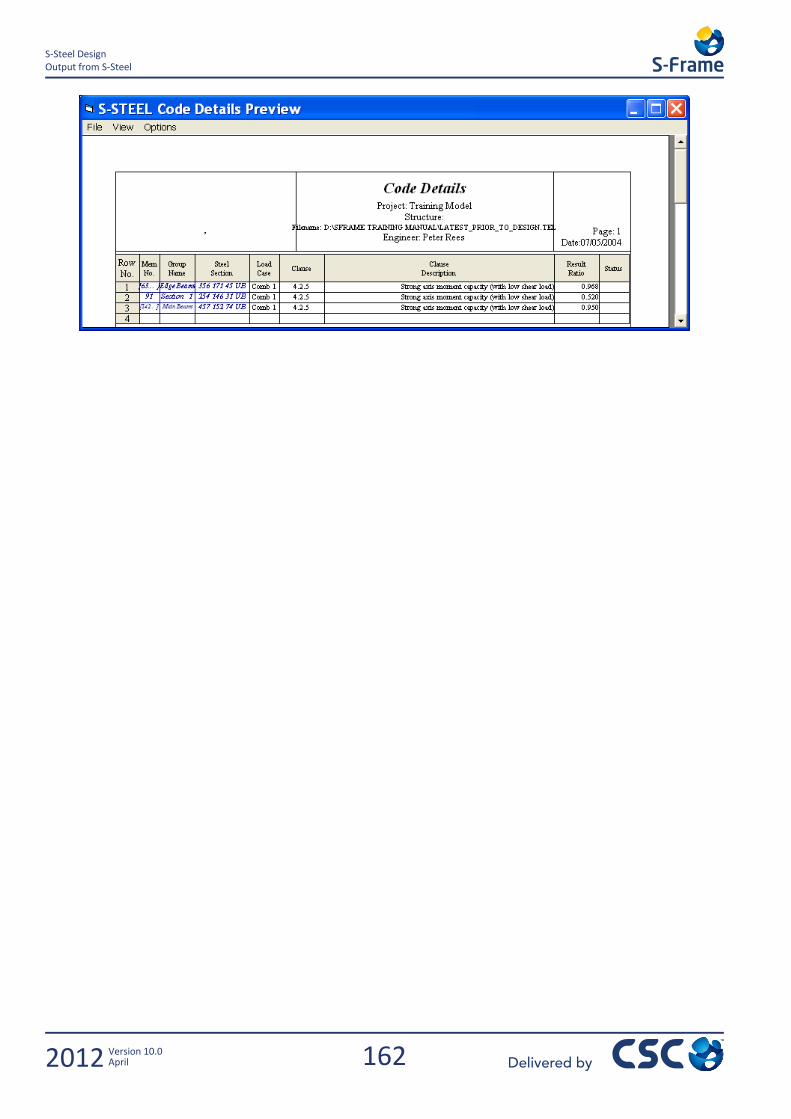
162
S-Steel Design Output from S-Steel
2012 Version 10.0 April
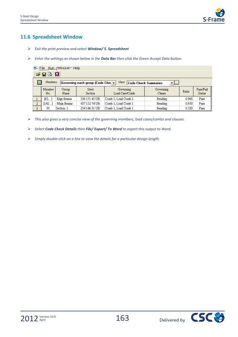
163
S-Steel Design Spreadsheet Window
2012 Version 10.0 April
11.6 Spreadsheet Window
Exit the print preview and select Window/ 5. Spreadsheet
Enter the settings as shown below in the Data Bar then click the Green Accept Data button
This also gives a very concise view of the governing members, load cases/combs and clauses.
Select Code Check Details then File/ Export/ To Word to export this output to Word.
Simply double-click on a line to view the details for a particular design length.
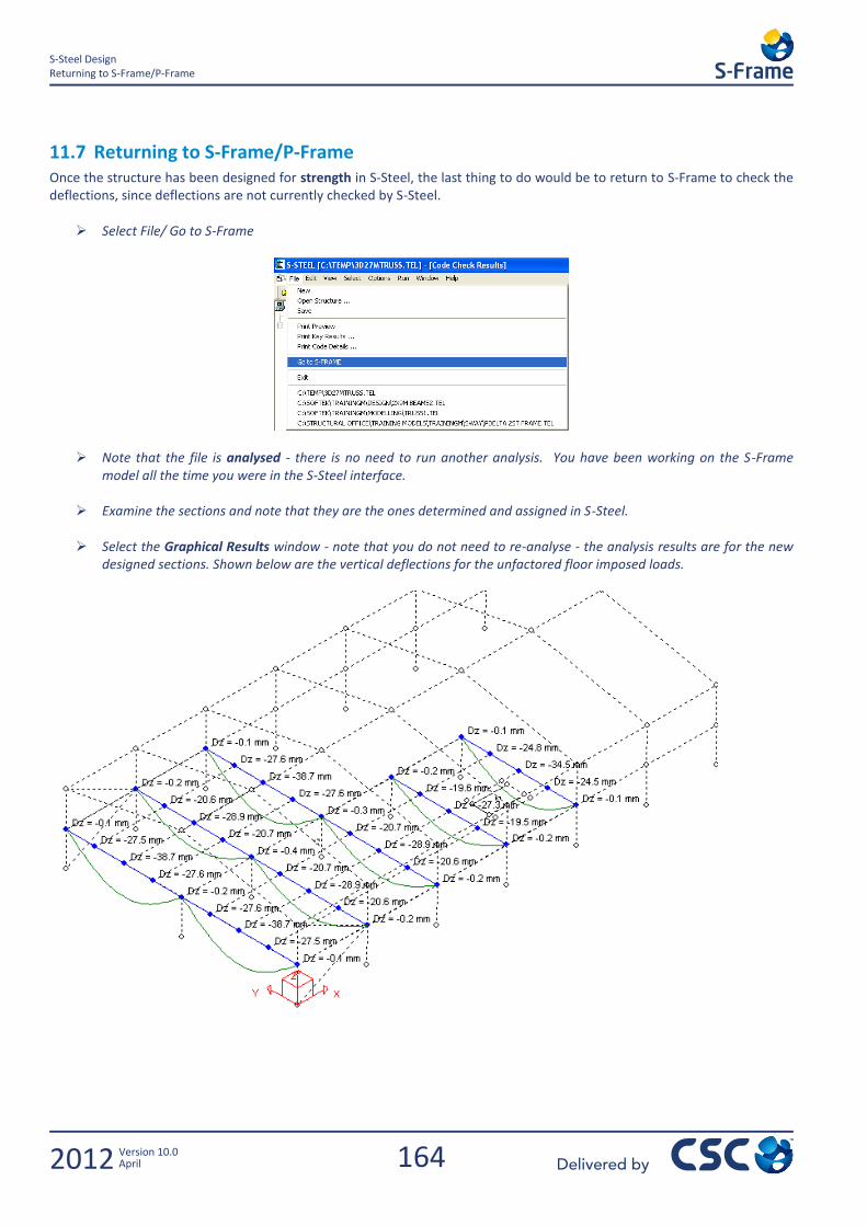
164
S-Steel Design Returning to S-Frame/P-Frame
2012 Version 10.0 April
11.7 Returning to S-Frame/P-Frame Once the structure has been designed for strength in S-Steel, the last thing to do would be to return to S-Frame to check the deflections, since deflections are not currently checked by S-Steel.
Select File/ Go to S-Frame
Note that the file is analysed - there is no need to run another analysis. You have been working on the S-Frame model all the time you were in the S-Steel interface.
Examine the sections and note that they are the ones determined and assigned in S-Steel.
Select the Graphical Results window - note that you do not need to re-analyse - the analysis results are for the new designed sections. Shown below are the vertical deflections for the unfactored floor imposed loads.

165
Alternative Modeling Methods Returning to S-Frame/P-Frame
2012 Version 10.0 April
12.0 Alternative Modeling Methods

166
Alternative Modeling Methods Enter Joints Using Joint Tool
2012 Version 10.0 April
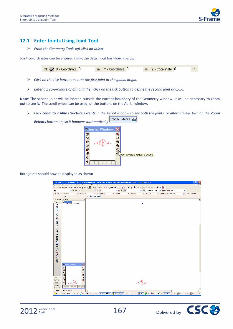
167
Alternative Modeling Methods Enter Joints Using Joint Tool
2012 Version 10.0 April
12.1 Enter Joints Using Joint Tool
From the Geometry Tools left click on Joints Joint co-ordinates can be entered using the data input bar shown below.
Click on the tick button to enter the first joint at the global origin.
Enter a Z co-ordinate of 6m and then click on the tick button to define the second joint at 0,0,6. Note: The second joint will be located outside the current boundary of the Geometry window. It will be necessary to zoom out to see it. The scroll wheel can be used, or the buttons on the Aerial window.
Click Zoom to visible structure extents in the Aerial window to see both the joints, or alternatively, turn on the Zoom
Extents button on, so it happens automatically
Both joints should now be displayed as shown
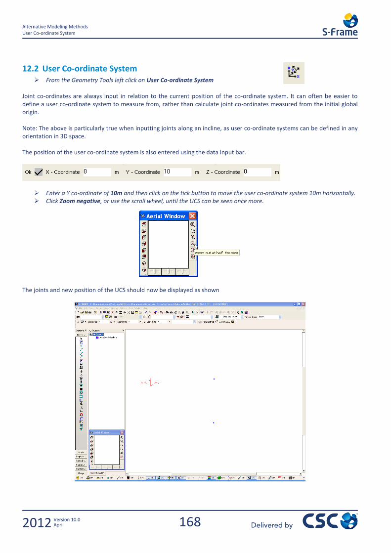
168
Alternative Modeling Methods User Co-ordinate System
2012 Version 10.0 April
12.2 User Co-ordinate System From the Geometry Tools left click on User Co-ordinate System
Joint co-ordinates are always input in relation to the current position of the co-ordinate system. It can often be easier to define a user co-ordinate system to measure from, rather than calculate joint co-ordinates measured from the initial global origin. Note: The above is particularly true when inputting joints along an incline, as user co-ordinate systems can be defined in any orientation in 3D space. The position of the user co-ordinate system is also entered using the data input bar.
Enter a Y co-ordinate of 10m and then click on the tick button to move the user co-ordinate system 10m horizontally. Click Zoom negative, or use the scroll wheel, until the UCS can be seen once more.
The joints and new position of the UCS should now be displayed as shown
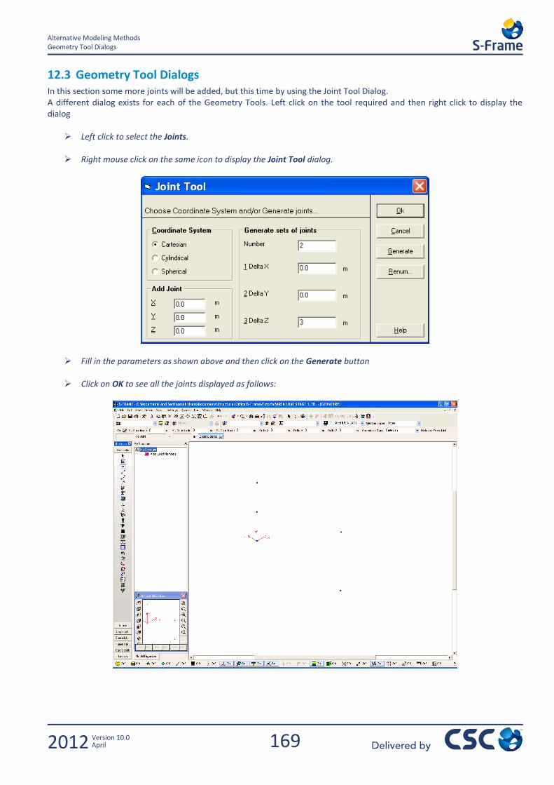
169
Alternative Modeling Methods Geometry Tool Dialogs
2012 Version 10.0 April
12.3 Geometry Tool Dialogs In this section some more joints will be added, but this time by using the Joint Tool Dialog. A different dialog exists for each of the Geometry Tools. Left click on the tool required and then right click to display the dialog
Left click to select the Joints.
Right mouse click on the same icon to display the Joint Tool dialog.
Fill in the parameters as shown above and then click on the Generate button
Click on OK to see all the joints displayed as follows:
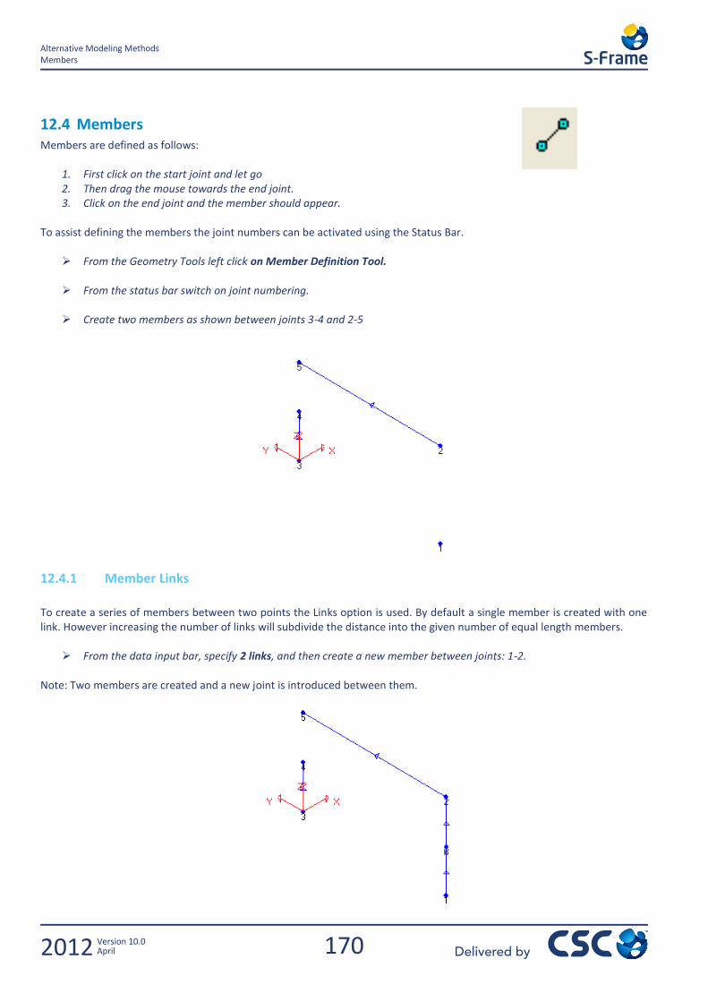
170
Alternative Modeling Methods Members
2012 Version 10.0 April
12.4 Members Members are defined as follows:
1. First click on the start joint and let go 2. Then drag the mouse towards the end joint. 3. Click on the end joint and the member should appear.
To assist defining the members the joint numbers can be activated using the Status Bar.
From the Geometry Tools left click on Member Definition Tool.
From the status bar switch on joint numbering.
Create two members as shown between joints 3-4 and 2-5
12.4.1 Member Links
To create a series of members between two points the Links option is used. By default a single member is created with one link. However increasing the number of links will subdivide the distance into the given number of equal length members.
From the data input bar, specify 2 links, and then create a new member between joints: 1-2. Note: Two members are created and a new joint is introduced between them.
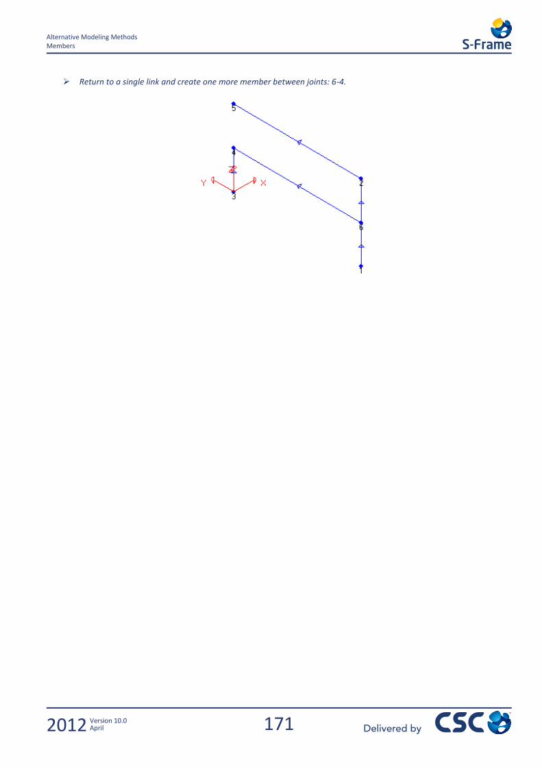
171
Alternative Modeling Methods Members
2012 Version 10.0 April
Return to a single link and create one more member between joints: 6-4.

172
Alternative Modeling Methods Move Commands
2012 Version 10.0 April
12.5 Move Commands Selected objects can be manipulated in a number of ways using the move commands.
Click on the Move icon that is located at the top of the screen, or from the Edit menu select Move.
12.5.1 Reflect
Choose the Reflect option and make the other settings as shown above. Then click on OK.
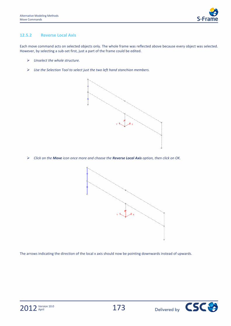
173
Alternative Modeling Methods Move Commands
2012 Version 10.0 April
12.5.2 Reverse Local Axis
Each move command acts on selected objects only. The whole frame was reflected above because every object was selected. However, by selecting a sub-set first, just a part of the frame could be edited.
Unselect the whole structure.
Use the Selection Tool to select just the two left hand stanchion members.
Click on the Move icon once more and choose the Reverse Local Axis option, then click on OK.
The arrows indicating the direction of the local x axis should now be pointing downwards instead of upwards.
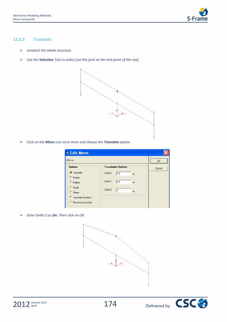
174
Alternative Modeling Methods Move Commands
2012 Version 10.0 April
12.5.3 Translate
Unselect the whole structure.
Use the Selection Tool to select just the joint at the mid-point of the roof.
Click on the Move icon once more and choose the Translate option.
Enter Delta Z as 2m. Then click on OK.

175
Alternative Modeling Methods Move Commands
2012 Version 10.0 April
Note: Although the joint was the only object selected, the members that are connected to the joint are stretched along with it.
Reselect the whole structure.
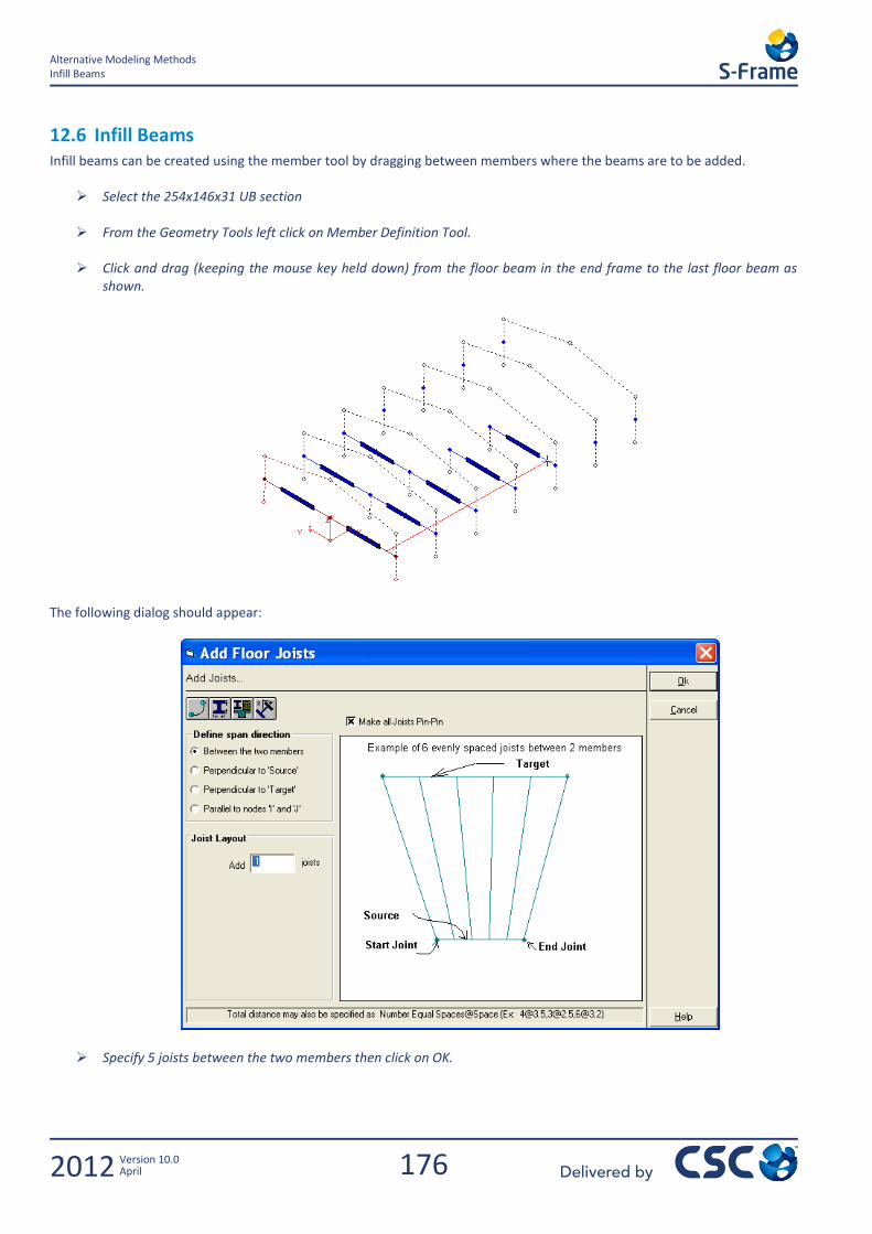
176
Alternative Modeling Methods Infill Beams
2012 Version 10.0 April
12.6 Infill Beams Infill beams can be created using the member tool by dragging between members where the beams are to be added.
Select the 254x146x31 UB section
From the Geometry Tools left click on Member Definition Tool.
Click and drag (keeping the mouse key held down) from the floor beam in the end frame to the last floor beam as shown.
The following dialog should appear:
Specify 5 joists between the two members then click on OK.
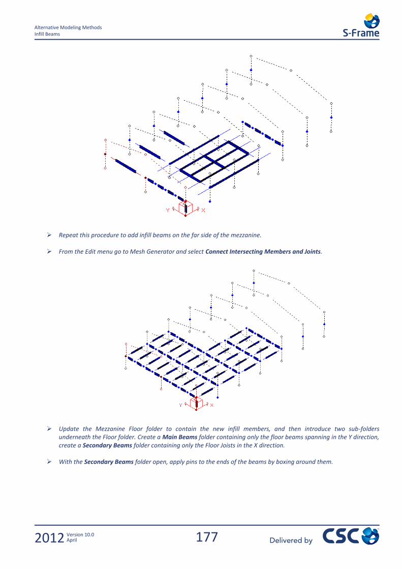
177
Alternative Modeling Methods Infill Beams
2012 Version 10.0 April
Repeat this procedure to add infill beams on the far side of the mezzanine.
From the Edit menu go to Mesh Generator and select Connect Intersecting Members and Joints.
Update the Mezzanine Floor folder to contain the new infill members, and then introduce two sub-folders underneath the Floor folder. Create a Main Beams folder containing only the floor beams spanning in the Y direction, create a Secondary Beams folder containing only the Floor Joists in the X direction.
With the Secondary Beams folder open, apply pins to the ends of the beams by boxing around them.
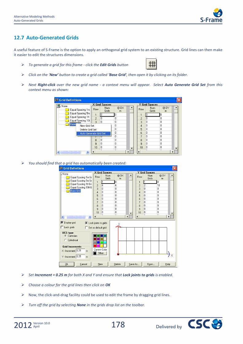
178
Alternative Modeling Methods Auto-Generated Grids
2012 Version 10.0 April
12.7 Auto-Generated Grids A useful feature of S-Frame is the option to apply an orthogonal grid system to an existing structure. Grid lines can then make it easier to edit the structures dimensions.
To generate a grid for this frame - click the Edit Grids button
Click on the ‘New’ button to create a grid called 'Base Grid', then open it by clicking on its folder.
Next Right-click over the new grid name - a context menu will appear. Select Auto Generate Grid Set from this context menu as shown:
You should find that a grid has automatically been created:
Set Increment = 0.25 m for both X and Y and ensure that Lock joints to grids is enabled.
Choose a colour for the grid lines then click on OK
Now, the click-and-drag facility could be used to edit the frame by dragging grid lines.
Turn off the grid by selecting None in the grids drop list on the toolbar.

CSC (UK) Ltd
Yeadon House, New Street Pudsey, Leeds LS28 8AQ United Kingdom
Tel: +44 (0) 113 239 3000Fax: +44 (0) 113 255 3917
[email protected] www.cscworld.com
© CSC (UK) Limited 2011. All Rights Reserved. Delivering:


