S. De and M. Baron. Step-up and step-down methods for...

S. De and M. Baron. Step-up and step-down methods for testing multiple

hypotheses in sequential experiments, J. of Stat. Planning and Inference,

142: 2059-2070, 2012.

Remark:

Tables 1 and 2 of this paper compare performance of our proposed procedures

with other methods. Results for the non-sequential Holm procedure and the

Bartroff–Lai multistage step-down procedure are taken from [38].

It should be noted that the ”sample size” of a clinical trial in Table 1 of [38] is

actually the total number of sampled components. Optimality of sequential

procedures in [38] is also measured in terms of the total number of sampled

components.

However, in our paper, the ”sample size” is defined as the number of sampled

patients. Therefore, our procedures are not to be compared with the Bartroff-

Lai rule.

Shyamal and Michael

1

Step-up and step-down methods for testing

multiple hypotheses in sequential experiments

Shyamal K. De and Michael Baron

Department of Mathematical Sciences, The University of Texas at Dallas,Richardson, TX 75080; [email protected], [email protected].

Abstract

Sequential methods are developed for testing multiple hypotheses, resulting

in a statistical decision for each individual test and controlling the familywise

error rate and the familywise power in the strong sense. Extending the ideas

of step-up and step-down methods for multiple comparisons to sequential

designs, the new techniques improve over the Bonferroni and closed testing

methods proposed earlier by a substantial reduction of the expected sample

size.

Keywords: Bonferroni methods, Familywise error rate, Holm procedure,

Sequential probability ratio test, Stopping boundaries, Wald approximation

2000 MSC: 62L, 62F03, 62H15

1. Introduction

1.1. Motivation

The problem of multiple inferences in sequential experiments arises in

many fields. Typical applications are in sequential clinical trials with both

efficacy and safety endpoints ([1]) or several outcome measures of efficacy

([2], [3]), acceptance sampling with several different criteria of acceptance

Preprint submitted to Journal of Statistical Planning and Inference 2012

([4], [5]), multichannel change-point detection ([6], [7]) and in microarray

experiments ([8]). It is often necessary to find the statistical answer to each

posed question by testing each individual hypothesis rather than giving one

global answer by combining all the tests into one and testing a composite

hypothesis.

Methods developed in this article aim to test multiple hypotheses based

on sequentially collected data, resulting in individual decisions for each in-

dividual test. They control the familywise error rate and the familywise

power in the strong sense. That is, both probabilities of rejecting at least

one true null hypothesis and accepting at least one false null hypothesis are

kept within the chosen levels α and β under any set of true hypotheses. This

condition is a multi-testing analogue of controlling both probabilities of Type

I and Type II errors in sequential experiments. As a result, the familywise

power, defined as the probability of detecting all significant differences at the

specified alternative parameter values, is controlled at the level (1− β) (see

[9] for three alternative definitions of familywise power).

Under these conditions, proposed stopping rules and decision rules achieve

substantial reduction of the expected sample size over all the existing (to the

best of our knowledge) sequential multiple testing procedures.

1.2. Sequential multiple comparisons in the literature

The concept of multiple comparisons is not new in sequential analysis.

Sequential methods exist for inferences about multivariate parameters ([10],

sec. 6.8 and 7.5). They are widely used in studies where inferences about

individual parameters are not required.

3

Most of the research in sequential multiple testing is limited to two types

of problems.

One type is the study of several (k > 2) treatments comparing their

effects. Sampled units are randomized to k groups where treatments are ad-

ministered. Based on the observed responses, one typically tests a composite

null hypothesis H0 : θ1 = . . . = θk against HA : not H0, where θj is the

effect of treatment j for j = 1, . . . , k ([11], [12], [13], [14], [15], chap. 16,

[16], [17], [18], [19], chap. 8). Sometimes each treatment is compared to the

accepted standard (e.g., [20]), and often the ultimate goal is selection of the

best treatment ([21], [22]).

The other type of studies involves a sequentially observed sequence of

data that needs to be classified into one of several available sets of models.

In a parametric setting, a null hypothesis H0 : θ ∈ Θ0 is tested against

several alternatives, H1 : θ ∈ Θ1 vs ... vs Hk : θ ∈ Θk, where θ is the

common parameter of the observed sequence ([23], [24], [25], [26]).

The optimal stopping rules for such tests are (naturally!) extensions of

the classical Wald’s sequential probability ratio tests ([27], [28], [29], [30]).

For the case of three alternative hypotheses, Sobel and Wald ([31]) obtained

a set of four stopping boundaries for the likelihood-ratio statistic. Their

solution was generalized to a larger number of alternatives resulting in the

multi-hypothesis sequential probability ratio tests ([32], [33]).

1.3. Our goal - simultaneous testing of individual hypotheses

The focus of this paper is different and more general. We assume that the

sequence of sampled units is observed to answer several questions about its

parameters. Indeed, once the sampling cost is already spent on each sampled

4

unit, it is natural to use it to answer more than just one question! Therefore,

there are d individual hypotheses about parameters θ1, . . . , θd of sequentially

observed vectors X1,X2, . . .,

H(1)0 : θ1 ∈ Θ01 vs H

(1)A : θ1 ∈ Θ11,

H(2)0 : θ2 ∈ Θ02 vs H

(2)A : θ2 ∈ Θ12,

· · ·

H(d)0 : θk ∈ Θ0d vs H

(d)A : θk ∈ Θ1d.

(1)

A few sequential procedures have been proposed for multiple tests similar

to (1). One can conduct individual sequential tests of H(1)0 , . . . , H

(d)0 and stop

after the first rejection or acceptance, as in [15], chap. 15. Hypotheses that

are not rejected at this moment will be accepted, conservatively protecting

the familywise Type I error rate (FWER-I).

Alternatively, one can assign level αj and the corresponding Pocock or

O’Brien-Fleming rejection boundary to the jth hypothesis. Then one con-

ducts sequential or group sequential tests in a hierarchical manner, as pro-

posed in [34], [35], and [36] for testing primary, secondary, and possibly

tertiary endpoints of a clinical trial. This procedure controls FWER-I at the

level α =∑

αj.

A different approach proposed in [37] and further developed in [38] allows

to control FWER-I by testing a closed set of hypotheses. Along with the

individual hypotheses H(1)0 , . . . , H

(d)0 , this method requires to test all the

composite hypotheses consisting of intersections ∩H(jk)0 , 1 ≤ jk ≤ d, 1 ≤ k ≤

d. This results in mandatory testing of (2d − 1) instead of d hypotheses. As

shown in Section 4, controlling the overall familywise Type I error rate will

then require a rather large expected sample size.

5

While focusing on the Type I FWER, these procedures do not control

the familywise Type II error rate and the familywise power. On the other

hand, a Type II error, for example, on one of the tests of a safety clinical trial

implies a failure to notice a side effect of a treatment, which is important to

control.

Notice that sequential tests of single hypotheses are able to control prob-

abilities of both the Type I and Type II errors. Extending this to multiple

testing, our goal is to control both familywise error rates I and II and to do

so at a low sampling cost by computing the optimal stopping boundaries and

the optimal stopping rule followed by the optimal terminal decisions.

1.4. Approach - extension of non-sequential ideas

To approach this problem, we use the step-up and step-down ideas de-

veloped for non-sequential multiple comparisons. Detailed overviews of non-

sequential methods were given at the NSF-CBMS Conference “New Horizons

in Multiple Comparison Procedures” in 2001 ([39]), in a 2008 monograph [40],

and at the 2009 Workshop on Modern Multiple Testing by Prof. S. Sarkar.

It was noted that the elementary Bonferroni adjustment for multiple com-

parisons takes care of the familywise error rate at the expense of power. How-

ever, some power can be regained by wisely designed step-up and step-down

methods, ordering p-values of individual tests, choosing one of the ordered

p-values, and proceeding from it into one or the other direction making deci-

sions on the acceptance or rejection of individual null hypotheses ([41], [42],

[43], [44], [45], [46], [47]).

Lehmann and Romano ([48]) introduced the generalized error rate, which

is the probability of making at least r incorrect inferences instead of at least

6

one. This weaker requirement on the error control allows to regain power in

studies with a large number of simultaneous inferences, where Bonferroni-

type adjustments result in very low significance levels and a great loss of

power. The new concept was quickly developed, and multiple comparison

methods controlling the generalized error rate were proposed ([49], [50], [51]).

Fixed-sample studies are able to control either the Type I or the Type II

error probabilities, but in general, not both. Conversely, Wald’s sequential

probability test and subsequent sequential procedures for testing a single

hypothesis can be designed to satisfy both the given significance level and the

given power. Similarly, sequential testing of multiple hypotheses, considered

here, can be set to guarantee a strong control of both familywise Type I and

Type II error rates,

FWER I = maxT ̸=∅

P {reject at least one true null hypothesis | T }

= maxT ̸=∅

P

{∪j∈T

reject H(j)0 | T

}(2)

FWERII = maxF̸=∅

P {accept at least one false null hypothesis | T }

= maxF̸=∅

P

∪j∈T̄

accept H(j)0 | T

(3)

where T ⊂ {1, . . . , d} is the index set of the true null hypotheses and F = T̄

is the index set of the false null hypotheses.

In the sequel, the non-sequential Bonferroni, step-down Holm, and step-

up Benjamini-Hochberg methods for multiple comparisons are generalized

to the sequential setting. Essentially, at every step of the multiple testing

scheme, the continue-sampling region is inserted between the acceptance and

7

rejection boundaries in such a way that the resulting sequential procedure

controls the intended error rate. Then, the so-called intersection stopping

rule is introduced that controls both familywise error rates simultaneously.

2. Sequential Bonferroni method

Let us begin with the rigorous formulation of the problem. Suppose a se-

quence of independent and identically distributed vectors X1,X2, . . . ∈ Rd

that are observed as a result of purely sequential or group sequential sam-

pling. Components (Xi1, . . . , Xid) of the i-th random vector may be de-

pendent, and the j-th component has a marginal density fj(· | θj) with

respect to a reference measure µj(·). For every j = 1, . . . , d, measures

{fj(· | θj), θj ∈ Θj} are assumed to be mutually absolutely continuous, and

the Kullback-Leibler information numbers

K(θj, θ′j) = Eθj log

{fj(Xj | θj)/fj(Xj | θ′j)

}are strictly positive and finite for θj ̸= θ′j.

Consider a battery of one-sided (right-tail, with a suitable parametriza-

tion) tests about parameters θ1, . . . , θd,

H(j)0 : θj ≤ θ

(j)0 vs. H

(j)A : θj ≥ θ

(j)1 , j = 1, . . . , d, (4)

A stopping rule T is to be found, accompanied with decision rules δj =

δj(X1j, . . . , XTj), j = 1, . . . , d, on the acceptance or rejection of each of the

null hypothesesH(1)0 , . . . , H

(d)0 . This procedure has to control both familywise

error rates (2) and (3), i.e., guarantee that

FWER I ≤ α and FWERII ≤ β (5)

8

for pre-assigned α, β ∈ (0, 1).

Technically, it is not difficult to satisfy condition (5). Wald’s sequential

probability ratio test (SPRT) for the j-th hypothesis controls the probabil-

ities of Type I and Type II errors at the given levels αj and βj. Choosing

αj = α/d and βj = β/d, we immediately obtain (5) by the Bonferroni in-

equality.

This testing procedure is based on log-likelihood ratios

Λ(j)n =

n∑i=1

logfj(Xij | θ(j)1 )

fj(Xij | θ(j)0 ), j = 1, . . . , d, n = 1, 2, . . . .

Wald’s classical stopping boundaries are

aj = log1− βj

αj

and bj = logβj

1− αj

. (6)

Wald’s SPRT for the single j-th hypothesis H(j)0 rejects it (i.e., chooses H

(j)A )

after n observations if Λ(j)n ≥ aj, accepts it (i.e., chooses H

(j)0 ) if Λ

(j)n ≤ bj,

and continues sampling if Λ(j)n ∈ (bj, aj).

Assuming that the marginal distributions of Λ(j)1 have the monotone like-

lihood ratio property (e.g. [52]), the error probabilities are maximized when

θj = θ(j)0 and when θj = θ

(j)1 , respectively, for all j = 1, . . . , d. Then, sepa-

rately performed SPRT for the j-th hypothesis with stopping boundaries (6)

controls the probabilities of Type I and Type II errors approximately,

P{Λ

(j)Tj

≥ aj | θj = θ(j)0

}≈ αj,

P{Λ

(j)Tj

≤ bj | θj = θ(j)1

}≈ βj,

(7)

where Tj = inf{n : Λ

(j)n ̸∈ (bj, aj)

}([53], [27], [28]). This Wald’s approxi-

mation ([54]) results from ignoring the overshoot over the stopping boundary

9

and assuming that having just crossed the stopping boundary for the first

time, the log-likelihood ratio Λ(j)n approximately equals to that boundary.

Extending SPRT to the case of multiple hypothesis, d ≥ 2, continue

sampling until all the d tests reach decisions. Define the stopping rule

T = inf

{n :

d∩j=1

{Λ(j)

n ̸∈ (bj, aj)}}

. (8)

Lemma 1. For any pairs (aj, bj), the stopping rule defined by (8) is proper.

Proof. Section 5.1.

Accepting or rejecting the j-th null hypothesis at time T depending on

whether Λ(j)T ≤ bj or Λ

(j)T ≥ aj, we could obtain (approximately, subject to

Wald’s approximation) a strong control of probabilities of Type I and Type

II errors by the Bonferroni inequality,

P {at least one Type I error} ≤d∑

j=1

P{Λ

(j)T ≥ aj

}≤

d∑j=1

αj = α;

P {at least one Type II error} ≤d∑

j=1

P{Λ

(j)T ≤ bj

}≤

d∑j=1

βj = β.

(9)

However, Wald’s approximation is only accurate when the overshoot of ΛT

over the stopping boundary is negligible. When testing d hypotheses, the

corresponding d log-likelihood ratios may cross their respective boundaries

at different times. Then, at the stopping time T , when sampling is halted, a

number of log-likelihood ratios may be deep inside the stopping region, cre-

ating a considerable overshoot. Wald’s approximation is no longer accurate

for the stopping time T ! It has to be replaced by rigorous statements.

10

Lemma 2. Let T be a proper stopping time with respect to the vector sequence

(X1,X2, . . .), such that

P{Λ

(j)T ∈ (b, a) | T

}= 0

for some j ∈ {1, . . . , d}, b < 0 < a, and any combination of true null

hypotheses T . Consider a test that rejects H(j)0 at time T if and only if

Λ(j)T ≥ a. For this test,

P{Type I error on H

(j)0

}≤ P

{Λ

(j)T ≥ a | θ(j)0

}≤ e−a, (10)

P{Type II error on H

(j)0

}≤ P

{Λ

(j)T ≤ b | θ(j)1

}≤ eb. (11)

Proof. Section 5.2.

Avoiding the use of Wald’s (and any other) approximation, replace Wald’s

stopping boundaries (6) for Λ(j)n by

aj = − logαj and bj = log βj (12)

and use the stopping rule (8). Then, according to Lemma 2, the correspond-

ing test of H(j)0 controls the Type I and Type II error probabilities rigorously

at levels e−aj = αj and ebj = βj. Therefore, by the Bonferroni arguments in

(9), the described multiple testing procedure controls both error rates. The

following theorem is then proved.

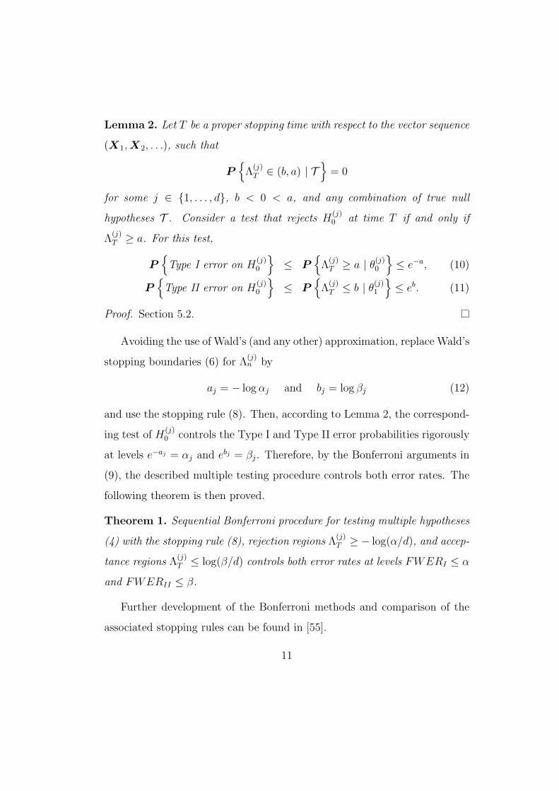
Theorem 1. Sequential Bonferroni procedure for testing multiple hypotheses

(4) with the stopping rule (8), rejection regions Λ(j)T ≥ − log(α/d), and accep-

tance regions Λ(j)T ≤ log(β/d) controls both error rates at levels FWERI ≤ α

and FWERII ≤ β.

Further development of the Bonferroni methods and comparison of the

associated stopping rules can be found in [55].

11

3. Step-down and step-up methods

Since Bonferroni methods are based on an inequality that appears rather

crude for moderate to large d, controlling both familywise rates I and II

can only be done at the expense of a large sample size. For non-sequential

statistical inferences, a number of elegant stepwise (step-up and step-down)

methods have been proposed, attaining the desired FWER-I and improving

over the Bonferroni methods in terms of the required sample size. In this

Section, we develop a similar approach for sequential experiments.

Following the Holm method for multiple comparisons (e.g., [56]), we or-

der the tested hypotheses H(1)0 , . . . , H

(d)0 according to the significance of the

collected evidence against them and set the significance levels for individual

tests to be

α1 =α

d, α2 =

α

d− 1, α3 =

α

d− 2, . . . , αj =

α

d+ 1− j, . . . , αd = α.

Similarly, in order to control the familywise Type II error rate, choose

βj =β

d+ 1− jfor j = 1, . . . , d.

Comparing with Bonferroni method, increasing the individual Type I and

Type II error probabilities has to cause the familywise error rates to increase.

On the other hand, since all the stopping boundaries become tighter, this will

necessarily reduce the expected sample size E(T ) under any combination of

true and false hypotheses, T and F . Therefore, if both rates can still be

controlled at the pre-specified levels α and β, then the resulting stepwise

procedure is an improvement of Bonferroni schemes under the given con-

straints on FWE rates.

12

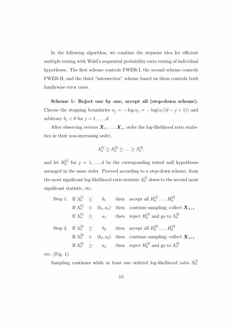
In the following algorithm, we combine the stepwise idea for efficient

multiple testing with Wald’s sequential probability ratio testing of individual

hypotheses. The first scheme controls FWER-I, the second scheme controls

FWER-II, and the third “intersection” scheme based on them controls both

familywise error rates.

Scheme 1: Reject one by one, accept all (step-down scheme).

Choose the stopping boundaries aj = − logαj = − log(α/(d − j + 1)) and

arbitrary bj < 0 for j = 1, . . . , d.

After observing vectors X1, . . . ,Xn, order the log-likelihood ratio statis-

tics in their non-increasing order,

Λ[1]n ≥ Λ[2]

n ≥ . . . ≥ Λ[d]n ,

and let H[j]0 for j = 1, . . . , d be the corresponding tested null hypotheses

arranged in the same order. Proceed according to a step-down scheme, from

the most significant log-likelihood ratio statistic Λ[1]n down to the second most

significant statistic, etc.

Step 1. If Λ[1]n ≤ b1 then accept all H

[1]0 . . . , H

[d]0

If Λ[1]n ∈ (b1, a1) then continue sampling; collect Xn+1

If Λ[1]n ≥ a1 then reject H

[1]0 and go to Λ

[2]n

Step 2. If Λ[2]n ≤ b2 then accept all H

[2]0 . . . , H

[d]0

If Λ[2]n ∈ (b2, a2) then continue sampling; collect Xn+1

If Λ[2]n ≥ a2 then reject H

[2]0 and go to Λ

[3]n

etc. (Fig. 1).

Sampling continues while at least one ordered log-likelihood ratio Λ[j]n

13

-

6

1 2 3 4 5 6 7 8 9 10

j

Λ[j]n = ordered log-likelihood ratios

aj =

∣∣∣∣log α

d− j + 1

∣∣∣∣

Arbitrary bj

t̀ `tHHt@@tAAAAt@@tJJJtAAAAt@@tPPt

-

6

1 2 3 4 5 6 7 8 9 10

j

Λ[j]n

aj =

∣∣∣∣log α

d− j + 1

∣∣∣∣

Arbitrary bj

t̀ t̀HHtXXtPPtXXtXXtEEEEEEEEEEEEtQ

QtPPtFigure 1: Example of Scheme 1. On the left, sampling continues. On the right, stop

sampling; reject H[1]0 , . . . , H

[7]0 ; accept H

[8]0 , . . . , H

[10]0 .

belongs to its continue-sampling region (bj, aj). The stopping rule corre-

sponding to this scheme is

T1 = inf

{n :

d∩j=1

Λ[j]n ̸∈ (bj, aj)

}. (13)

Theorem 2. The stopping rule T1 is proper; Scheme 1 strongly controls the

familywise Type I error rate. That is, for any set T of true hypotheses,

P T {T1 < ∞} = 1

and

P T {at least one Type I error} ≤ α. (14)

Proof. Section 5.3.

Theorem 2 holds for arbitrary bj < 0, thus it also shows that the rejection

boundary aj alone controls FWER-I.

14

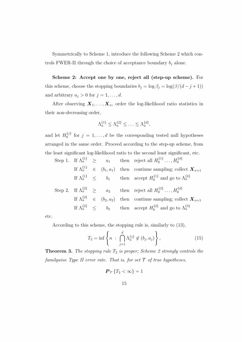
Symmetrically to Scheme 1, introduce the following Scheme 2 which con-

trols FWER-II through the choice of acceptance boundary bj alone.

Scheme 2: Accept one by one, reject all (step-up scheme). For

this scheme, choose the stopping boundaries bj = log βj = log(β/(d− j +1))

and arbitrary aj > 0 for j = 1, . . . , d.

After observing X1, . . . ,Xn, order the log-likelihood ratio statistics in

their non-decreasing order,

Λ{1}n ≤ Λ{2}

n ≤ . . . ≤ Λ{d}n ,

and let H{j}0 for j = 1, . . . , d be the corresponding tested null hypotheses

arranged in the same order. Proceed according to the step-up scheme, from

the least significant log-likelihood ratio to the second least significant, etc.

Step 1. If Λ{1}n ≥ a1 then reject all H

{1}0 . . . , H

{d}0

If Λ{1}n ∈ (b1, a1) then continue sampling; collect Xn+1

If Λ{1}n ≤ b1 then accept H

{1}0 and go to Λ

{2}n

Step 2. If Λ{2}n ≥ a2 then reject all H

{2}0 . . . , H

{d}0

If Λ{2}n ∈ (b2, a2) then continue sampling; collect Xn+1

If Λ{2}n ≤ b2 then accept H

{2}0 and go to Λ

{3}n

etc.

According to this scheme, the stopping rule is, similarly to (13),

T2 = inf

{n :

d∩j=1

Λ{j}n ̸∈ (bj, aj)

}, (15)

Theorem 3. The stopping rule T2 is proper; Scheme 2 strongly controls the

familywise Type II error rate. That is, for set T of true hypotheses,

P T {T2 < ∞} = 1

15

-

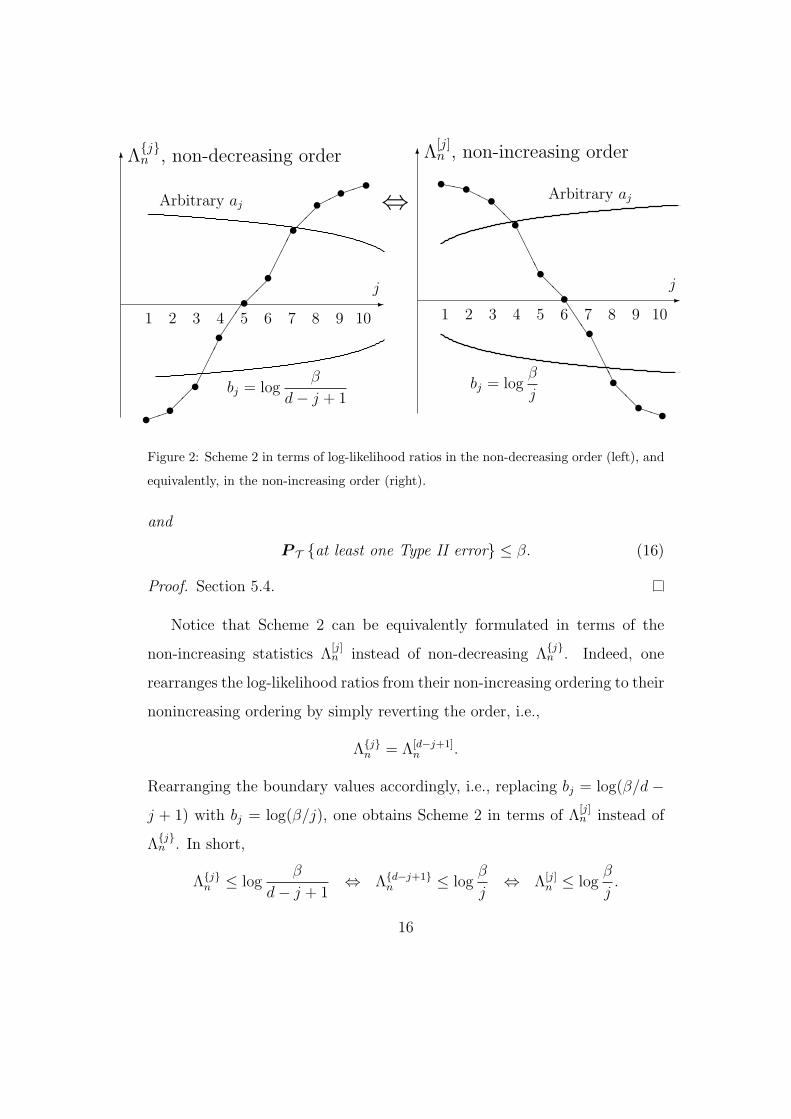
6

1 2 3 4 5 6 7 8 9 10

j

Λ{j}n , non-decreasing order

Arbitrary aj

bj = logβ

d− j + 1

tt��t��

t��

t��

t��

t

t��

t��t��

-

6

1 2 3 4 5 6 7 8 9 10

j

Λ[j]n , non-increasing order

Arbitrary aj

bj = logβ

j


⇔

Figure 2: Scheme 2 in terms of log-likelihood ratios in the non-decreasing order (left), and

equivalently, in the non-increasing order (right).

and

P T {at least one Type II error} ≤ β. (16)

Proof. Section 5.4.

Notice that Scheme 2 can be equivalently formulated in terms of the

non-increasing statistics Λ[j]n instead of non-decreasing Λ

{j}n . Indeed, one

rearranges the log-likelihood ratios from their non-increasing ordering to their

nonincreasing ordering by simply reverting the order, i.e.,

Λ{j}n = Λ[d−j+1]

n .

Rearranging the boundary values accordingly, i.e., replacing bj = log(β/d−

j + 1) with bj = log(β/j), one obtains Scheme 2 in terms of Λ[j]n instead of

Λ{j}n . In short,

Λ{j}n ≤ log

β

d− j + 1⇔ Λ{d−j+1}

n ≤ logβ

j⇔ Λ[j]

n ≤ logβ

j.

16

This is illustrated in Fig. 2.

Comparing the logic of Schemes 1 and 2, we see that the step-down

Scheme 1 starts with the most significant log-likelihood ratio statistic Λ[1]n

and carefully/conservatively rejects one null hypothesis at a time. It focuses

on controlling Type I errors of wrong rejection and results in controlling the

overall FWER-I.

On the contrary, the step-up Scheme 2 starts with the least significant

statistic and conservatively accepts one null at a time, controlling FWER-II.

It is actually possible to combine both schemes and to develop a sequential

procedure controlling both familywise error rates as follows.

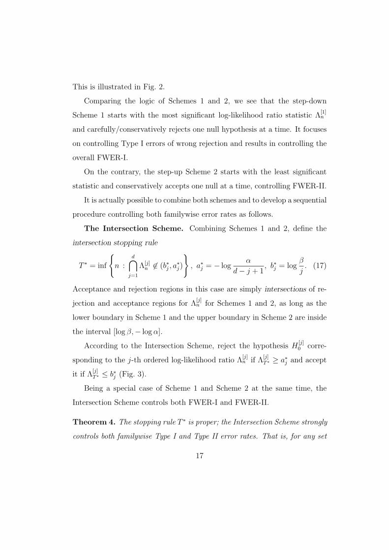
The Intersection Scheme. Combining Schemes 1 and 2, define the

intersection stopping rule

T ∗ = inf

{n :

d∩j=1

Λ[j]n ̸∈ (b∗j , a

∗j)

}, a∗j = − log

α

d− j + 1, b∗j = log

β

j. (17)

Acceptance and rejection regions in this case are simply intersections of re-

jection and acceptance regions for Λ[j]n for Schemes 1 and 2, as long as the

lower boundary in Scheme 1 and the upper boundary in Scheme 2 are inside

the interval [log β,− logα].

According to the Intersection Scheme, reject the hypothesis H[j]0 corre-

sponding to the j-th ordered log-likelihood ratio Λ[j]n if Λ

[j]T ∗ ≥ a∗j and accept

it if Λ[j]T ∗ ≤ b∗j (Fig. 3).

Being a special case of Scheme 1 and Scheme 2 at the same time, the

Intersection Scheme controls both FWER-I and FWER-II.

Theorem 4. The stopping rule T ∗ is proper; the Intersection Scheme strongly

controls both familywise Type I and Type II error rates. That is, for any set

17

-

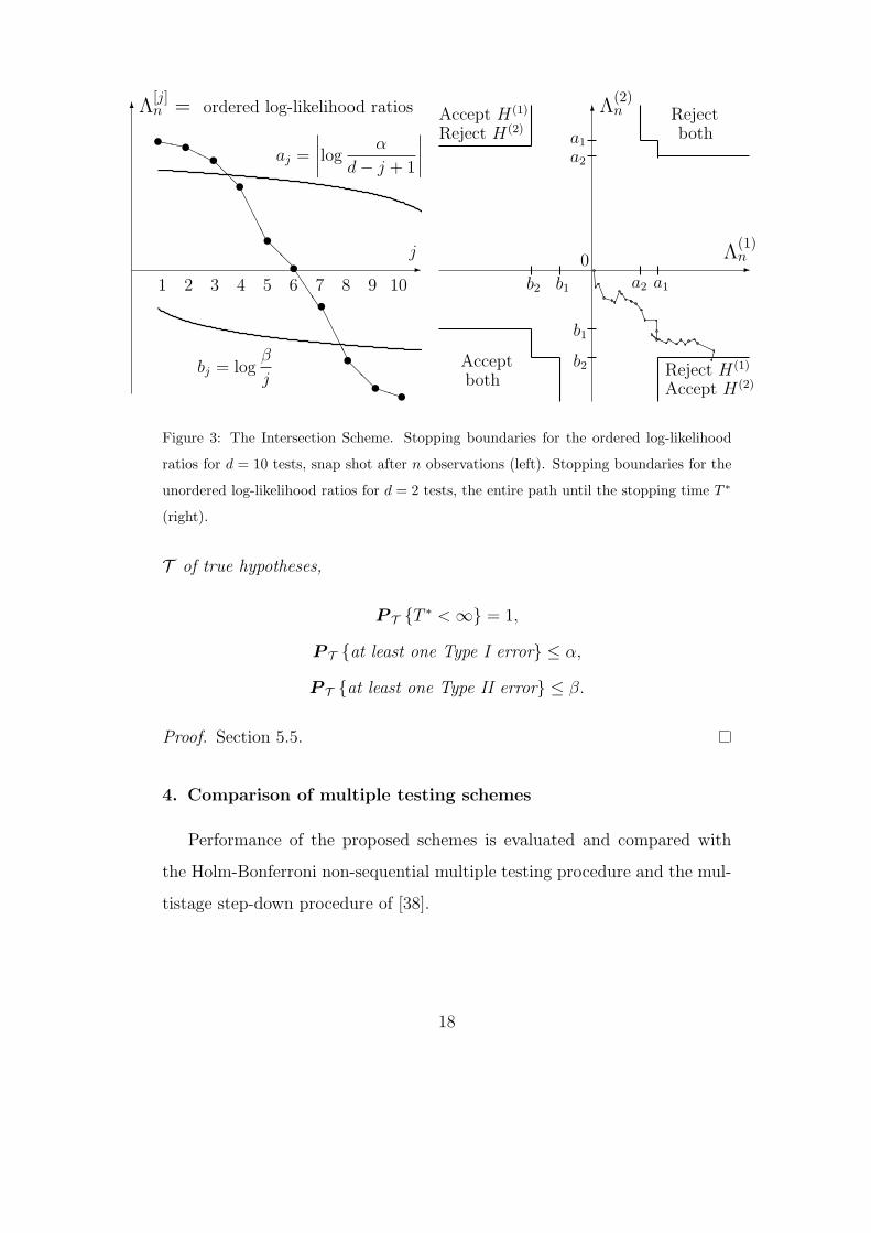
6

1 2 3 4 5 6 7 8 9 10

j

Λ[j]n = ordered log-likelihood ratios

aj =

∣∣∣∣log α

d− j + 1

∣∣∣∣

bj = logβ

j


6

-

Acceptboth

Reject H(1)

Accept H(2)

Rejectboth

Accept H(1)

Reject H(2)

b2

b1

a2a1

b2 b1 a2 a1

0 Λ(1)n

Λ(2)n

Figure 3: The Intersection Scheme. Stopping boundaries for the ordered log-likelihood

ratios for d = 10 tests, snap shot after n observations (left). Stopping boundaries for the

unordered log-likelihood ratios for d = 2 tests, the entire path until the stopping time T ∗

(right).

T of true hypotheses,

P T {T ∗ < ∞} = 1,

P T {at least one Type I error} ≤ α,

P T {at least one Type II error} ≤ β.

Proof. Section 5.5.

4. Comparison of multiple testing schemes

Performance of the proposed schemes is evaluated and compared with

the Holm-Bonferroni non-sequential multiple testing procedure and the mul-

tistage step-down procedure of [38].

18

First, consider testing three null hypotheses,

H(1)0 : θ1 = 0 vs H

(1)A : θ1 = 0.5,

H(2)0 : θ2 = 0 vs H

(2)A : θ2 = 0.5,

H(3)0 : θ3 = 0.5 vs H

(3)A : θ3 = 0.75,

based on a sequence of random vectorsX1,X2, . . ., whereX i = (Xi1, Xi2, Xi3),

Xi1 ∼ Normal(θ1, 1), Xi2 ∼ Normal(θ2, 1), and Xi3 ∼ Bernoulli(θ3), which

is the scenario considered in [38].

For each combination of null hypotheses and alternatives, N = 55, 000

random sequences are simulated (omitting the combinationsH(1)A ∩H(2)

0 ∩H(3)0

and H(1)A ∩H

(2)0 ∩H

(3)A , because of their interchangeability with H

(1)0 ∩H

(2)A ∩

H(3)0 and H

(1)0 ∩H

(2)A ∩H

(3)A , respectively, therefore yielding exactly the same

performance of the considered stopping and decision rules). Based on them,

the familywise Type I and Type II error rates are estimated along with

the expected stopping time and the standard error of our estimator of the

expected stopping time. Scheme 1 and the Intersection Scheme are set to

control FWERI ≤ 0.05. Also, Scheme 2 and the Intersection Scheme are set

to control FWERII ≤ 0.10.

Results are shown in Tables 1-2. It can be seen that under each com-

bination of true null hypotheses, the expected sample sizes of sequential

Bonferroni, step-down Scheme 1, step-up Scheme 2, and the Intersection

Scheme are of the same order; however, they are about a half of the expected

size of the closed testing procedure or the fixed-sample size required by the

non-sequential Holm-Bonferroni procedure.

Advantage of stepwise schemes versus the sequential Bonferroni scheme

19

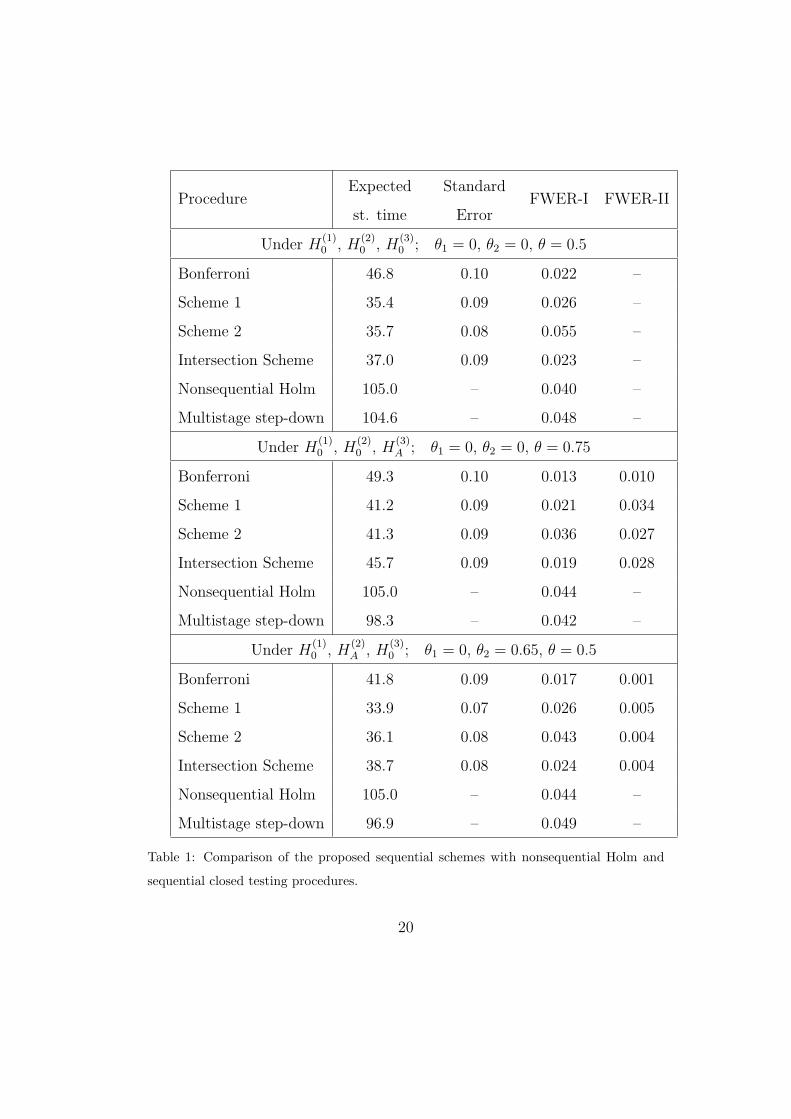
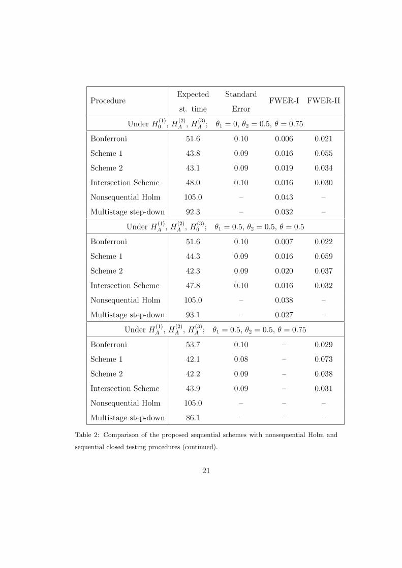
ProcedureExpected

st. time

Standard

ErrorFWER-I FWER-II

Under H(1)0 , H

(2)0 , H

(3)0 ; θ1 = 0, θ2 = 0, θ = 0.5

Bonferroni 46.8 0.10 0.022 –

Scheme 1 35.4 0.09 0.026 –

Scheme 2 35.7 0.08 0.055 –

Intersection Scheme 37.0 0.09 0.023 –

Nonsequential Holm 105.0 – 0.040 –

Multistage step-down 104.6 – 0.048 –

Under H(1)0 , H

(2)0 , H

(3)A ; θ1 = 0, θ2 = 0, θ = 0.75

Bonferroni 49.3 0.10 0.013 0.010

Scheme 1 41.2 0.09 0.021 0.034

Scheme 2 41.3 0.09 0.036 0.027

Intersection Scheme 45.7 0.09 0.019 0.028



Under H(1)0 , H

(2)A , H

(3)0 ; θ1 = 0, θ2 = 0.65, θ = 0.5

Bonferroni 41.8 0.09 0.017 0.001

Scheme 1 33.9 0.07 0.026 0.005

Scheme 2 36.1 0.08 0.043 0.004




Table 1: Comparison of the proposed sequential schemes with nonsequential Holm and

sequential closed testing procedures.

20

ProcedureExpected

st. time

Standard

ErrorFWER-I FWER-II

Under H(1)0 , H

(2)A , H

(3)A ; θ1 = 0, θ2 = 0.5, θ = 0.75

Bonferroni 51.6 0.10 0.006 0.021

Scheme 1 43.8 0.09 0.016 0.055

Scheme 2 43.1 0.09 0.019 0.034




Under H(1)A , H

(2)A , H

(3)0 ; θ1 = 0.5, θ2 = 0.5, θ = 0.5

Bonferroni 51.6 0.10 0.007 0.022

Scheme 1 44.3 0.09 0.016 0.059

Scheme 2 42.3 0.09 0.020 0.037




Under H(1)A , H

(2)A , H

(3)A ; θ1 = 0.5, θ2 = 0.5, θ = 0.75

Bonferroni 53.7 0.10 – 0.029

Scheme 1 42.1 0.08 – 0.073

Scheme 2 42.2 0.09 – 0.038

Intersection Scheme 43.9 0.09 – 0.031

Nonsequential Holm 105.0 – – –

Multistage step-down 86.1 – – –

Table 2: Comparison of the proposed sequential schemes with nonsequential Holm and

sequential closed testing procedures (continued).

21

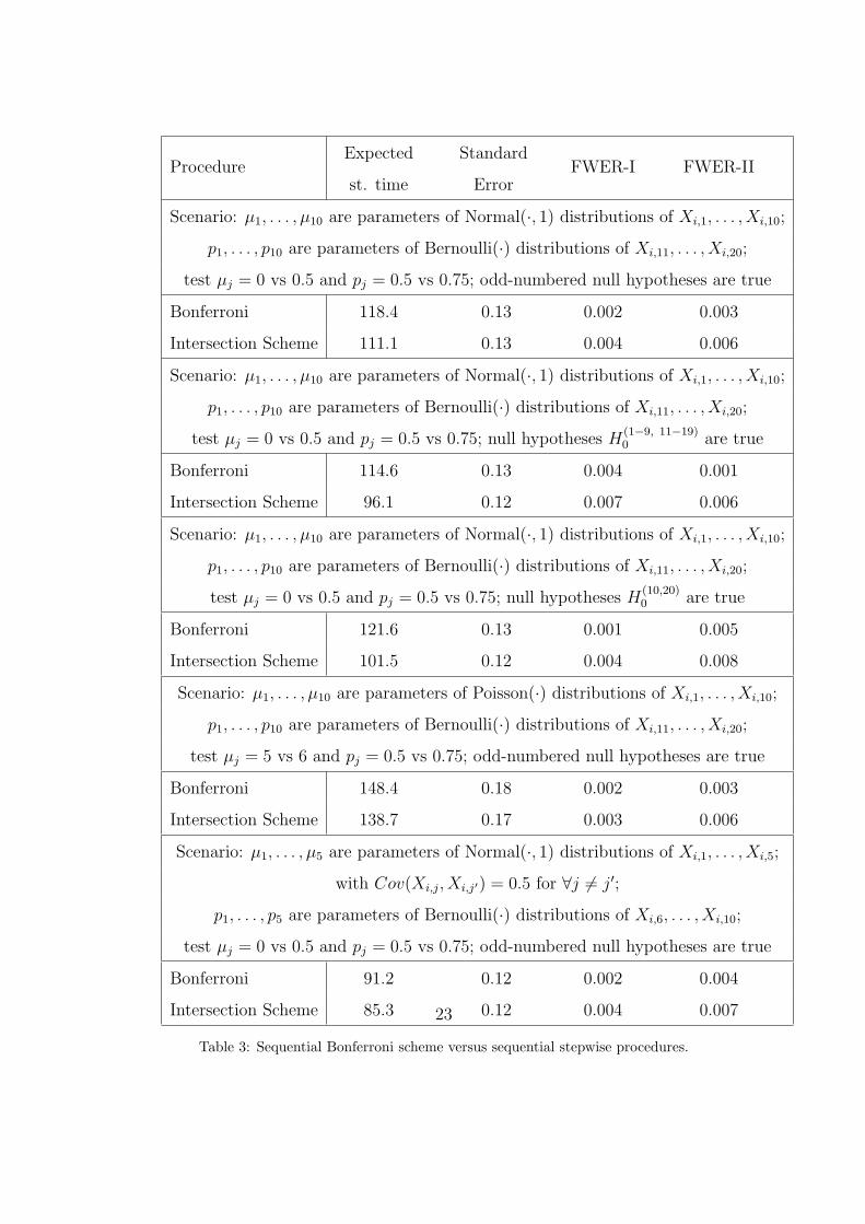
is more significant for a larger number of tests. This is seen in Table 3 for

different multiple testing problems. Reduction in the expected sample size

ranges from 6% when 50% of null hypotheses are true to 16.5% when most

null hypotheses are either true or false. Results are also based on N = 55, 000

simulated sequences for each considered scenario.

The last example in Table 3 deals with correlated components of the

observed random vectors. Indeed, all the results in this article make no as-

sumption about the joint distribution of (Xi1, . . . , Xid) for each i = 1, 2, . . ..

When components are correlated, positively or negatively, the expected sam-

ple size of each procedure should reduce.

We also notice that results of Theorems 1-4 are based on Bonferroni-

type inequalities and corollaries from them. For a large number of tests,

Bonferroni inequality tends to be rather crude, and therefore, the familywise

error rates, guaranteed by Theorems 1-4, are often satisfied with a rather

wide margin. This certainly leaves room for the improvement of the proposed

sequential testing schemes!

5. Appendix: Proofs

5.1. Proof of Lemma 1

By the weak law of large numbers,

P{Λ(j)

n ∈ (bj, aj) | H(j)0

}→ 0 and P

{Λ(j)

n ∈ (bj, aj) | H(j)A

}→ 0, as n → ∞,

because the non-zero expected values of Λ(j)n are guaranteed by the assump-

tions of Section 2 on Kullback-Leibler information numbers. Then

P T {T > n} ≤d∑

j=1

P T{Λ(j)

n ∈ (bj, aj)}→ 0,

22

ProcedureExpected

st. time

Standard

ErrorFWER-I FWER-II

Scenario: µ1, . . . , µ10 are parameters of Normal(·, 1) distributions of Xi,1, . . . , Xi,10;

p1, . . . , p10 are parameters of Bernoulli(·) distributions of Xi,11, . . . , Xi,20;

test µj = 0 vs 0.5 and pj = 0.5 vs 0.75; odd-numbered null hypotheses are true

Bonferroni 118.4 0.13 0.002 0.003




test µj = 0 vs 0.5 and pj = 0.5 vs 0.75; null hypotheses H(1−9, 11−19)0 are true

Bonferroni 114.6 0.13 0.004 0.001




test µj = 0 vs 0.5 and pj = 0.5 vs 0.75; null hypotheses H(10,20)0 are true

Bonferroni 121.6 0.13 0.001 0.005


Scenario: µ1, . . . , µ10 are parameters of Poisson(·) distributions of Xi,1, . . . , Xi,10;


test µj = 5 vs 6 and pj = 0.5 vs 0.75; odd-numbered null hypotheses are true

Bonferroni 148.4 0.18 0.002 0.003



with Cov(Xi,j, Xi,j′) = 0.5 for ∀j ̸= j′;


test µj = 0 vs 0.5 and pj = 0.5 vs 0.75; odd-numbered null hypotheses are true

Bonferroni 91.2 0.12 0.002 0.004


Table 3: Sequential Bonferroni scheme versus sequential stepwise procedures.

23

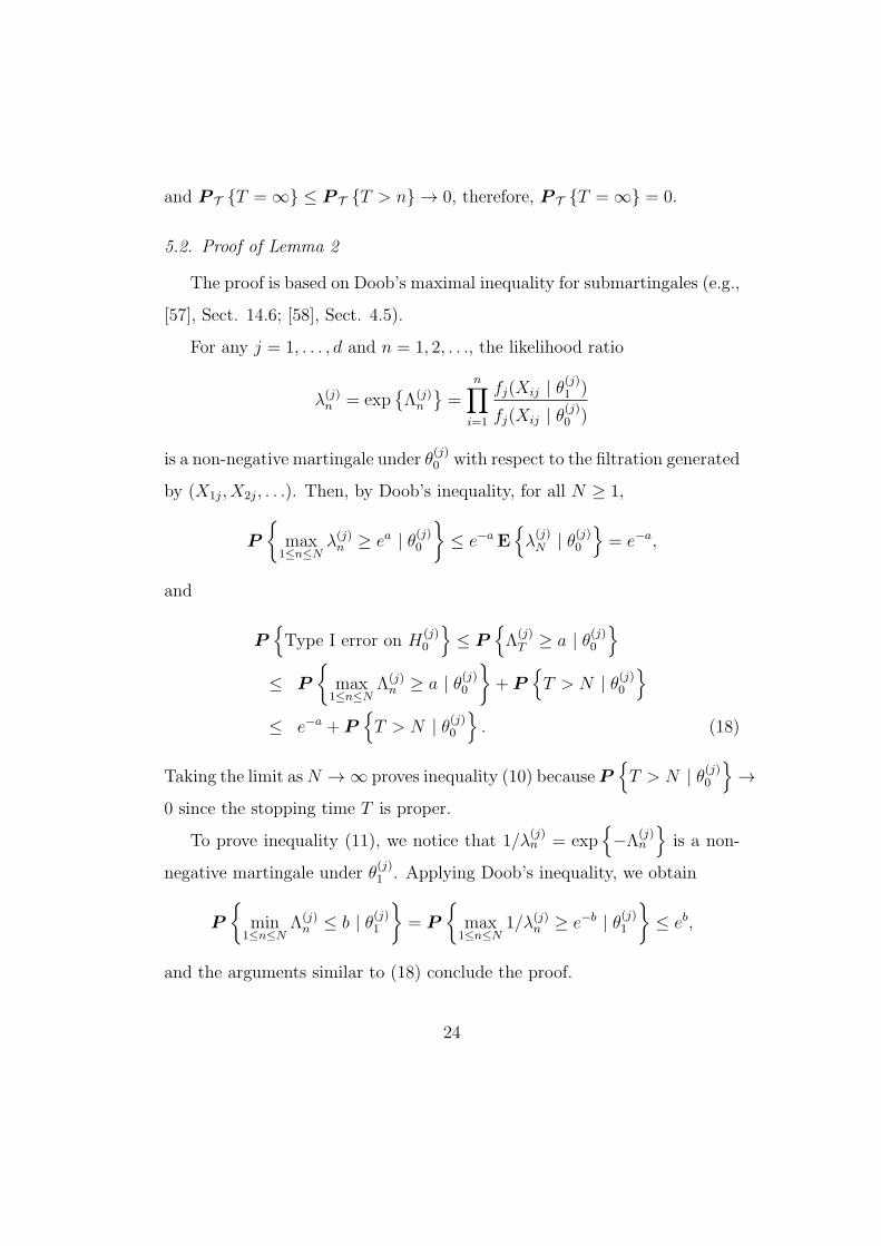
and P T {T = ∞} ≤ P T {T > n} → 0, therefore, P T {T = ∞} = 0.

5.2. Proof of Lemma 2

The proof is based on Doob’s maximal inequality for submartingales (e.g.,

[57], Sect. 14.6; [58], Sect. 4.5).

For any j = 1, . . . , d and n = 1, 2, . . ., the likelihood ratio

λ(j)n = exp

{Λ(j)

n

}=

n∏i=1

fj(Xij | θ(j)1 )

fj(Xij | θ(j)0 )

is a non-negative martingale under θ(j)0 with respect to the filtration generated

by (X1j, X2j, . . .). Then, by Doob’s inequality, for all N ≥ 1,

P

{max

1≤n≤Nλ(j)n ≥ ea | θ(j)0

}≤ e−a E

{λ(j)N | θ(j)0

}= e−a,

and

P{Type I error on H

(j)0

}≤ P

{Λ

(j)T ≥ a | θ(j)0

}≤ P

{max

1≤n≤NΛ(j)

n ≥ a | θ(j)0

}+ P

{T > N | θ(j)0

}≤ e−a + P

{T > N | θ(j)0

}. (18)

Taking the limit asN → ∞ proves inequality (10) becauseP{T > N | θ(j)0

}→

0 since the stopping time T is proper.

To prove inequality (11), we notice that 1/λ(j)n = exp

{−Λ

(j)n

}is a non-

negative martingale under θ(j)1 . Applying Doob’s inequality, we obtain

P

{min

1≤n≤NΛ(j)

n ≤ b | θ(j)1

}= P

{max

1≤n≤N1/λ(j)

n ≥ e−b | θ(j)1

}≤ eb,

and the arguments similar to (18) conclude the proof.

24

5.3. Proof of Theorem 2

1. The stopping time T1 is almost surely bounded by

T ′ = inf

{n :

d∩j=1

{Λ(j)

n ̸∈ (min bj,max aj)}}

. (19)

Since T ′ is proper by Lemma 1, so is T1.

2. The proof of control of FWER-I borrows ideas from the classical deriva-

tion of the experimentwise error rate of the non-sequential Holm procedure,

extending the arguments to sequential tests.

Let T ⊂ {1, . . . , d} be the index set of true null hypotheses, and F = T̄

be the index set of the false null hypotheses, with cardinalities |T | and |F|.

Then, arrange the log-likelihood ratios at the stopping time T1 in their non-

increasing order, Λ[1]T1

≥ . . . ≥ Λ[d]T1

and let m be the smallest index of the

ordered log-likelihood ratio that corresponds to a true hypothesis. In other

words, if H[j]0 denotes the null hypothesis that is being tested by the log-

likelihood ratio Λ[j]T1

for j = 1, . . . , d, then m is such that all H[j]0 are false for

j < m whereas H[m]0 is true. Thus, there are at least (m−1) false hypotheses,

so that m− 1 ≤ |F| = d− |T |.

No Type I error can be made on false hypotheses H[1]0 , . . . , H

[m−1]0 . If

the Type I error is not made on H[m]0 either, then there is no Type I error

at all because according to Scheme 1, acceptance of H[m]0 implies automatic

acceptance of the remaining hypotheses H[m+1]0 , . . . , H

[d]0 .

Therefore,

P T {at least one Type I error} = P T

{Λ

[m]T1

≥ am

}≤ P T

{Λ

[m]T1

≥ ad−|T |+1

}= P T

{maxj∈T Λ

(j)T1

≥ ad−|T |+1

}≤

∑j∈T P T

{Λ

(j)T1

≥ ad−|T |+1

}.

25

Recall that rejection boundaries for Scheme 1 are chosen as aj = − logαj,

where αj = α/(d + 1 − j). Therefore, ad−|T |+1 = − log(α/|T |), and by

Lemma 2,

PH

(j)0

{Λ

(j)T1

≥ ad−|T |+1

}≤ exp

{−ad−|T |+1

}= α/|T |.

Finally, we have

P T {at least one Type I error} ≤∑j∈T

α/|T | = α.

5.4. Main steps of the proof of Theorem 3

Ideas of Section 5.3 are now translated to Scheme 2 and control of FWER-

II. Let us outline the main steps of the proof, especially because control of

FWER-II has not been studied in sequential multiple testing, to the best of

our knowledge.

1. Similarly to T1, the stopping time T2 is also bounded by the proper

stopping rule (19), and therefore, it is also proper.

2. Following Scheme 2, arrange Λ(j)T2

in their non-decreasing order, Λ{1}T2

≤

. . . ≤ Λ{d}T2

. Then let ℓ be the smallest index of the ordered log-likelihood

ratio that corresponds to a false null hypothesis, so that all H{1}0 , . . . , H

{ℓ−1}0 ,

corresponding to Λ{1}T2

, . . . ,Λ{ℓ−1}T2

, are true but H{ℓ}0 is false. The number of

true hypotheses is then at least (ℓ − 1), so that ℓ ≤ |T | + 1 = d − |F| + 1,

where |T | and |F| are the numbers of true and false null hypotheses.

If any Type II error is made during Scheme 2, then it has to occur on

H{ℓ}0 , because its (correct) rejection leads to the automatic (correct) rejection

of the remaining hypotheses H{ℓ+1}0 , . . . , H

{d}0 , according to the scheme.

26

Therefore, applying (11) to Λ(j)T2, we obtain

FWERII = P T

{Λ

{ℓ}T2

≤ bℓ

}≤ P T

{Λ

{ℓ}T2

≤ bd−|F|+1

}= P T

{minj∈F

Λ(j)T2

≤ bd−|F|+1

}≤

∑j∈F

P T

{Λ

(j)T2

≤ log(β/|F|)}≤

∑j∈F

β/|F| = β.

5.5. Proof of Theorem 4

The intersection scheme satisfies all the conditions of Theorem 2, there-

fore, the stopping time T ∗ is proper, and the scheme controls FWERI ≤

α. At the same time, it satisfies Theorem 3, and therefore, it controls

FWERII ≤ β.

6. Acknowledgements

The authors are grateful to the Editor Professor N. Balakrishnan, the

Associate Editor, and to the anonymous referee for deep, insightful, and en-

couraging comments that helped us tremendously. Research of both authors

is funded by the National Science Foundation grant DMS 1007775. Research

of the second author is partially supported by the National Security Agency

grant H98230-11-1-0147. This funding is greatly appreciated.

References

[1] C. Jennison and B. W. Turnbull, Group sequential tests for bivariate

response: Interim analyses of clinical trials with both efficacy and safety

endpoints, Biometrics 49 (1993) 741–752.

27

[2] P. C. O’Brien, Procedures for comparing samples with multiple end-

points, Biometrics 40 (1984) 1079–1087.

[3] S. J. Pocock, N. L. Geller, and A. A. Tsiatis, The analysis of multiple

endpoints in clinical trials, Biometrics 43 (1987) 487–498.

[4] D. H. Baillie, Multivariate acceptance sampling - some applications to

defence procurement, The Statistician 36 (1987) 465–478.

[5] D. C. Hamilton, M. L. Lesperance, A consulting problem involving bi-

variate acceptance sampling by variables, Canadian J. Stat. 19 (1991)

109–117.

[6] A. G. Tartakovsky, V. V. Veeravalli, Change-point detection in multi-

channel and distributed systems with applications, in: N. Mukhopad-

hyay, S. Datta and S. Chattopadhyay, Eds., Applications of Sequential

Methodologies, Marcel Dekker, Inc., New York, 2004, pp. 339–370.

[7] A. G. Tartakovsky, X. R. Li, and G. Yaralov, Sequential detection of

targets in multichannel systems, IEEE Trans. Information Theory 49 (2)

(2003) 425–445.

[8] S. Dudoit, J. P. Shaffer, and J. C. Boldrick, Multiple hypothesis testing

in microarray experiment, Stat. Science 18 (2003) 71–103.

[9] J. P. Shaffer, Multiple hypothesis testing, Annual Review of Psychology

46 (1995) 561–584.

[10] M. Ghosh, N. Mukhopadhyay and P. K. Sen, Sequential Estimation,

Wiley, New York, 1997.

28

[11] R. A. Betensky, An O’Brien-Fleming sequential trial for comparing three

treatments, Ann. Stat. 24 (4) (1996) 1765–1791.

[12] D. Edwards, Extended-Paulson sequential selection, Ann. Stat. 15 (1)

(1987) 449–455.

[13] D. G. Edwards, J. C. Hsu, Multiple comparisons with the best treat-

ment, J. Amer. Stat. Assoc. 78 (1983) 965–971.

[14] M. D. Hughes, Stopping guidelines for clinical trials with multiple treat-

ments, Statistics in Medicine 12 (1993) 901–915.

[15] C. Jennison and B. W. Turnbull, Group sequential methods with appli-

cations to clinical trials, Chapman & Hall, Boca Raton, FL, 2000.

[16] P. C. O’Brien, T. R. Fleming, A multiple testing procedure for clinical

trials, Biometrika 35 (1979) 549–556.

[17] D. Siegmund, A sequential clinical trial for comparing three treatments,

Ann. Stat. 21 (1993) 464–483.

[18] R. R. Wilcox, Extention of Hochberg’s two-stage multiple comparison

method, in: N. Mukhopadhyay, S. Datta and S. Chattopadhyay, Eds.,

Applications of Sequential Methodologies, Marcel Dekker, Inc., New

York, 2004, pp. 371–380.

[19] S. Zacks, Stage-wise Adaptive Designs, Wiley, Hoboken, NJ, 2009.

[20] E. Paulson, A sequential procedure for comparing several experimental

categories with a standard or control, Ann. Math. Stat. 33 (1962) 438–

443.

29

[21] C. Jennison, I. M. Johnstone, and B. W. Turnbull, Asymptotically op-

timal procedures for sequential adaptive selection of the best of several

normal means, in: S. S. Gupta and J. O. Berger, eds., Statistical Deci-

sion Theory and Related Topics III, Vol. 2, Academic Press, New York,

1982, pp. 55–86.

[22] E. Paulson, A sequential procedure for selecting the population with the

largest mean from k normal populations, Ann. Math. Stat. 35 (1964)

174–180.

[23] P. Armitage, Sequential analysis with more than two alternative hy-

potheses, and its relation to discriminant function analysis, J. Roy.

Statist. Soc. B 12 (1950) 137–144.

[24] C. W. Baum, V. V. Veeravalli, A sequential procedure for multihypoth-

esis testing, IEEE Trans. Inform. Theory 40 (1994) 1994–2007.

[25] A. Novikov, Optimal sequential multiple hypothesis tests, Kybernetika

45 (2) (2009) 309–330.

[26] G. Simons, Lower bounds for the average sample number of sequential

multihypothesis tests, Ann. Math. Stat. 38 (5) (1967) 1343–1364.

[27] Z. Govindarajulu, Sequential Statistics, World Scientific Publishing Co,

Singapore, 2004.

[28] A. Wald, Sequential Analysis, Wiley, New York, 1947.

[29] A. Wald, J. Wolfowitz, Optimal character of the sequential probability

ratio test, Ann. Math. Statist. 19 (1948) 326–339.

30

[30] D. Siegmund, Sequential Analysis: Tests and Confidence Intervals,

Springer-Verlag, New York, 1985.

[31] M. Sobel, A. Wald, A sequential decision procedure for choosing one of

three hypotheses concerning the unknown mean of a normal distribution,

Ann. Math. Stat. 20 (4) (1949) 502–522.

[32] V. P. Dragalin, A. G. Tartakovsky, and V. V. Veeravalli, Multihypothesis

sequential probability ratio tests. Part I: Asymptotic optimality, IEEE

Trans. Inform. Theory 45 (7) (1999) 2448–2461.

[33] T. L. Lai, Sequential multiple hypothesis testing and efficient fault

detection-isolation in stochastic systems, IEEE Trans. Inform. Theory

46 (2) (2000) 595–608.

[34] E. Glimm, W. Maurer, and F. Bretz, Hierarchical testing of multiple

endpoints in group-sequential trials, Statistics in Medicine 29 (2010)

219–228.

[35] A. C. Tamhane, C. R. Mehta, and L. Liu, Testing a primary and a

secondary endpoint in a group sequential design, Biometrics 66 (2010)

1174–1184.

[36] W. Maurer, E. Glimm, and F. Bretz, Multiple and repeated testing of

primary, coprimary, and secondary hypotheses, Statistics in Biopharma-

ceutical Research 3 (2) (2011) 336–352.

[37] D.-I. Tang and N. L. Geller, Closed testing procedures for group se-

quential clinical trials with multiple endpoints, Biometrics 55 (1999)

1188–1192.

31

[38] J. Bartroff and T.-L. Lai, Multistage tests of multiple hypotheses, Com-

munications in Statistics - Theory and Methods 39 (2010) 1597–1607.

[39] Y. Benjamini, F. Bretz, and S. Sarkar, Eds., Recent Developments in

Multiple Comparison Procedures, IMS Lecture Notes - Monograph Se-

ries, Beachwood, Ohio, 2004.

[40] S. Dudoit, M. J. van der Laan, Multiple Testing Procedures with Ap-

plications to Genomics, Springer, New York, 2008.

[41] Y. Benjamini, Y. Hochberg, Controlling the false discovery rate: a prac-

tical and powerful approach to multiple testing, J. Royal Stat. Soc. 57 (1)

(1995) 289–300.

[42] Y. Hochberg, A. C. Tamhane, Multiple comparison procedures, Wiley,

New York, 1987.

[43] S. Holm, A simple sequentially rejective multiple test procedure, Scand.

J. Stat. 6 (1979) 65–70.

[44] S. K. Sarkar, Some probability inequalities for ordered mtp2 random

variables: a proof of the simes conjecture, Ann. Stat. 26 (2) (1998) 494–

504.

[45] S. K. Sarkar, Some results on false discovery rate in stepwise multiple

testing procedures, Ann. Stat. 30 (1) (2002) 239–257.

[46] Z. Sidak, Rectangular confidence regions for the means of multivariate

normal distributions, J. Amer. Statist. Assoc. 62 (1967) 626–633.

32

[47] R. J. Simes, An improved Bonferroni procedure for multiple tests of

significance, Biometrika 73 (1986) 751–754.

[48] E. L. Lehmann, J. P. Romano, Generalizations of the familywise error

rate, Ann. Stat. 33 (2005) 1138–1154.

[49] J. P. Romano, M. Wolf, Control of generalized error rates in multiple

testing, Ann. Stat. 35 (2007) 1378–1408.

[50] S. K. Sarkar, Step-up procedures controlling generalized FWER and

generalized FDR, Ann. Stat. 35 (2007) 2405–2420.

[51] S. K. Sarkar, W. Guo, On a generalized false discovery rate, Ann. Stat.

37 (3) (2009) 1545–1565.

[52] G. Casella and R. L. Berger, Statistical Inference, Duxbury Press, Bel-

mont, CA, 2002.

[53] Z. Govindarajulu, The Sequential Statistical Analysis of Hypothesis

Testing, Point and Interval Estimation, and Decision Theory, Ameri-

can Sciences Press, Columbus, Ohio, 1987.

[54] M. Basseville, I. V. Nikiforov, Detection of Abrupt Changes: Theory

and Application, PTR Prentice-Hall, Inc., 1993.

[55] S. De and M. Baron, Sequential bonferroni methods for multiple hy-

pothesis testing with strong control of familywise error rates I and II,

Sequential Analysis (in press).

[56] J. Neter, M. Kutner, C. Nachtsheim and W. Wasserman, Applied Linear

Statistical Models, 4th ed., McGraw-Hill, 1996.

33

[57] D. Williams, Probability with Martingales, Cambridge University Press,

Cambridge, UK, 1991.

[58] H. H. Kuo, Introduction to Stochastic Integration, Springer, New York,

2006.

34

S. De and M. Baron. Step-up and step-down methods for...

Documents

Transcript of S. De and M. Baron. Step-up and step-down methods for...