S. BROVERMAN STUDY GUIDE FOR THE SOCIETY … 3MLC-BRO-12SSM-P... SOA Exam MLC Study Guide © S....

www.sambroverman.com SOA Exam MLC Study Guide © S. Broverman 2012

S. BROVERMAN STUDY GUIDE

FOR THE

SOCIETY OF ACTUARIESEXAM MLC

2012 EDITION

EXCERPTS

Samuel Broverman, ASA, PHD

[email protected]

copyright © 2012, S. Broverman


Excerpts:

Table of Contents

Introductory Note

Section 5 - Models for Survival and Mortality

Practice Exam 1 and Solutions


S. BROVERMAN EXAM MLC STUDY GUIDE - VOLUME 1NOTES, EXAMPLES AND PROBLEM SETS

Introductory Note

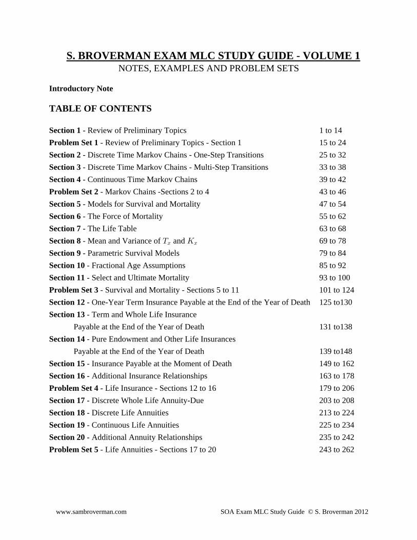
TABLE OF CONTENTS

Section 1 - Review of Preliminary Topics 1 to 14

Problem Set 1 - Review of Preliminary Topics - Section 1 15 to 24

Section 2 - Discrete Time Markov Chains - One-Step Transitions 25 to 32

Section 3 - Discrete Time Markov Chains - Multi-Step Transitions 33 to 38

Section 4 - Continuous Time Markov Chains 39 to 42

Problem Set 2 - Markov Chains -Sections 2 to 4 43 to 46

Section 5 - Models for Survival and Mortality 47 to 54

Section 6 - The Force of Mortality 55 to 62

Section 7 - The Life Table 63 to 68

Section 8 - Mean and Variance of and 69 to 78X OB B

Section 9 - Parametric Survival Models 79 to 84

Section 10 - Fractional Age Assumptions 85 to 92

Section 11 - Select and Ultimate Mortality 93 to 100

Problem Set 3 - Survival and Mortality - Sections 5 to 11 101 to 124

Section 12 - One-Year Term Insurance Payable at the End of the Year of Death 125 to130

Section 13 - Term and Whole Life Insurance

Payable at the End of the Year of Death 131 to138

Section 14 - Pure Endowment and Other Life Insurances

Payable at the End of the Year of Death 139 to148

Section 15 - Insurance Payable at the Moment of Death 149 to 162

Section 16 - Additional Insurance Relationships 163 to 178

Problem Set 4 - Life Insurance - Sections 12 to 16 179 to 206

Section 17 - Discrete Whole Life Annuity-Due 203 to 208

Section 18 - Discrete Life Annuities 213 to 224

Section 19 - Continuous Life Annuities 225 to 234

Section 20 - Additional Annuity Relationships 235 to 242

Problem Set 5 - Life Annuities - Sections 17 to 20 243 to 262


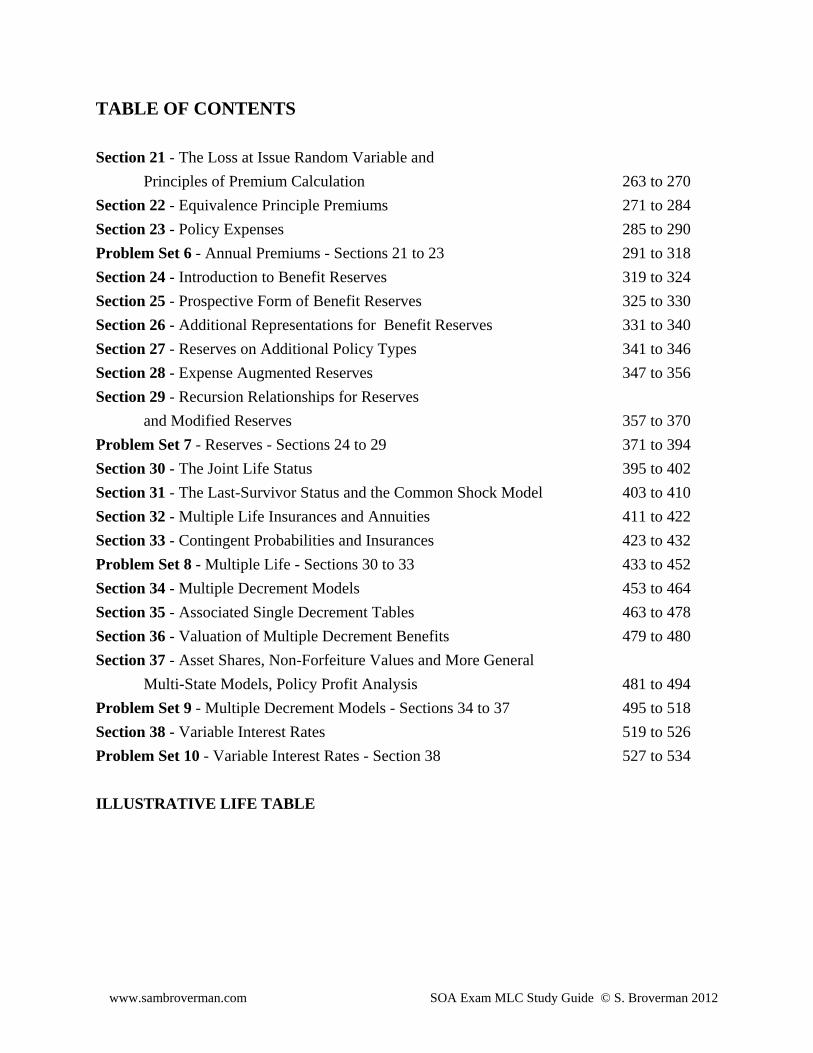
TABLE OF CONTENTS

Section 21 - The Loss at Issue Random Variable and

Principles of Premium Calculation 263 to 270

Section 22 - Equivalence Principle Premiums 271 to 284

Section 23 - Policy Expenses 285 to 290

Problem Set 6 - Annual Premiums - Sections 21 to 23 291 to 318

Section 24 - Introduction to Benefit Reserves 319 to 324

Section 25 - Prospective Form of Benefit Reserves 325 to 330

Section 26 - Additional Representations for Benefit Reserves 331 to 340

Section 27 - Reserves on Additional Policy Types 341 to 346

Section 28 - Expense Augmented Reserves 347 to 356

Section 29 - Recursion Relationships for Reserves

and Modified Reserves 357 to 370

Problem Set 7 - Reserves - Sections 24 to 29 371 to 394

Section 30 - The Joint Life Status 395 to 402

Section 31 - The Last-Survivor Status and the Common Shock Model 403 to 410

Section 32 - Multiple Life Insurances and Annuities 411 to 422

Section 33 - Contingent Probabilities and Insurances 423 to 432

Problem Set 8 - Multiple Life - Sections 30 to 33 433 to 452

Section 34 - Multiple Decrement Models 453 to 464

Section 35 - Associated Single Decrement Tables 463 to 478

Section 36 - Valuation of Multiple Decrement Benefits 479 to 480

Section 37 - Asset Shares, Non-Forfeiture Values and More General

Multi-State Models, Policy Profit Analysis 481 to 494

Problem Set 9 - Multiple Decrement Models - Sections 34 to 37 495 to 518

Section 38 - Variable Interest Rates 519 to 526

Problem Set 10 - Variable Interest Rates - Section 38 527 to 534

ILLUSTRATIVE LIFE TABLE


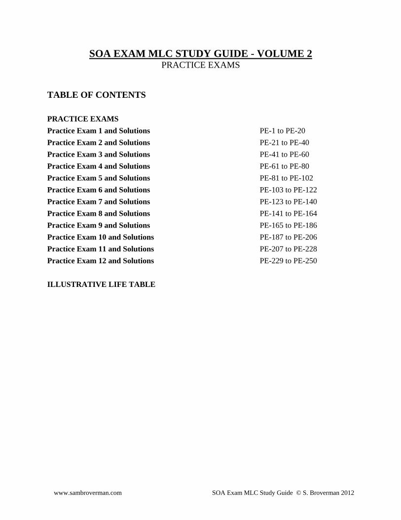
SOA EXAM MLC STUDY GUIDE - VOLUME 2PRACTICE EXAMS

TABLE OF CONTENTS

PRACTICE EXAMS

Practice Exam 1 and Solutions PE-1 to PE-20












ILLUSTRATIVE LIFE TABLE


INTRODUCTORY NOTE

This study guide is designed to help in the preparation for Exam MLC of the Society ofActuaries (the life contingencies and probability exam).

The study guide is divided into two volumes. Volume 1 consists of review notes, examples andproblem sets. Volume 2 contains 12 practice exams of 30 questions each. There are over 170examples in the notes, over 360 problems in the problem sets and 360 questions in the 12practice exams. All of these (almost 900) questions have detailed solutions. The notes are brokenup into 38 sections Each section has a suggested approximate time frame.

Most of the examples in the notes and about half of the problems in the problem sets are fromolder SOA or CAS exams on the relevant topics. The practice exams have 30 questions each andare designed to be similar to actual 3-hour exams. Some of the questions on the practice examsare variations on actual exam questions. The SOA has posted on its website a sample questionfile for Exam MLC with solutions. Many of those questions are from old exams, and there maybe some overlap in the questions found in this study guide and those found in the SOA files, butI have attempted to limit that duplication. The SOA and CAS questions are copyrighted by theSOA and CAS, and I gratefully acknowledge that I have been permitted to include them in thisstudy guide.

Because of the time constraint on the exam, a crucial aspect of exam taking is the ability to workquickly. I believe that working through many problems and examples is a good way to build upthe speed at which you work. It can also be worthwhile to work through problems that havebeen done before, as this helps to reinforce familiarity, understanding and confidence. Workingmany problems will also help in being able to more quickly identify topic and question types. Ihave attempted, wherever possible, to emphasize shortcuts and efficient and systematic ways ofsetting up solutions. There are also occasional comments on interpretation of the language usedin some exam questions. While the focus of the study guide is on exam preparation, from time totime there will be comments on underlying theory in places that I feel those comments mayprovide useful insight into a topic.

It has been my intention to make this study guide self-contained and comprehensive for all ExamMLC topics, but there are may be occasional references to the books listed in the SOA examcatalog. While the ability to derive formulas used on the exam is usually not the focus of anexam question, it is useful in enhancing the understanding of the material and may be helpful inmemorizing formulas. There may be an occasional reference in the review notes to a derivation,but you are encouraged to review the official reference material for more detail on formuladerivations.

In order for the review notes in this study guide to be most effective, you should have somebackground at the junior or senior college level in probability and statistics. It will be assumedthat you are reasonably familiar with differential and integral calculus.


Of the various calculators that are allowed for use on the exam, I think that theBA II PLUS is probably the best choice. It has several memories and has good financialfunctions. I think that the TI-30X IIS would be the second best choice.

There is a set of tables that has been provided with the exam in past sittings. These tables consistof a standard normal distribution probability table and a life table. The tables are available fordownload from the Society of Actuaries website, but are included at the ends of both Volumes 1and 2 for convenience.

If you have any questions, comments, criticisms or compliments regarding this study guide, youmay contact me at the address below. I apologize in advance for any errors, typographical orotherwise, that you might find, and it would be greatly appreciated if you would bring them tomy attention. I will be maintaining a website for errata that can be accessed fromwww.sambroverman.com . It is my sincere hope that you find this study guide helpful and usefulin your preparation for the exam. I wish you the best of luck on the exam.

Samuel A. Broverman February, 2012Department of StatisticsUniversity of Toronto100 St. George StreetToronto, Ontario CANADA M5S 3G3 E-mail: [email protected] or [email protected]: www.sambroverman.com


MLC SECTION 5 - MODELS FOR SURVIVAL AND MORTALITYMQR CHAPTER 5

The suggested time frame for covering this section is 2 hours.

The Survival Function

A standard way of describing survival and mortality is by using a random variable for the time

from birth until death. When an individual is born, the time until death is a random variable. The

Bowers book defines the following: time until death, or age at death of a newborn.\ œ X œ \!

is a continuous, positive random variable ( ). The of is\ ! \distribution function

J ÐBÑ œ J ÐBÑ œ T<Ò\ Ÿ BÓ œ T ÒX Ÿ BÓ\ ! !

probability that the newborn dies before or on attaining age .œ B

The or of issurvival function survival distribution function \

=ÐBÑ œ "J ÐBÑ œ T<Ò\ BÓ œ W ÐBÑ œ "J ÐBÑ\ ! !

œ Bprobability that the newborn dies after attaining age ,

the probability that the newborn survives to at least age .œ B

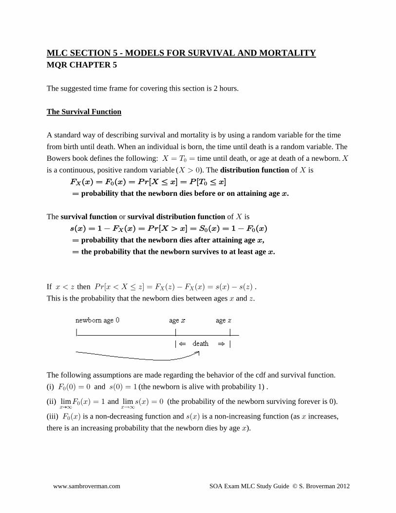
If then .B D T<ÒB \ Ÿ DÓ œ J ÐDÑ J ÐBÑ œ =ÐBÑ =ÐDÑ\ \

This is the probability that the newborn dies between ages and .B D

The following assumptions are made regarding the behavior of the cdf and survival function.

(i) and (the newborn is alive with probability 1) .J Ð!Ñ œ ! =Ð!Ñ œ "!

(ii) and (the probability of the newborn surviving forever is 0).lim limBp∞ BÄ∞

!J ÐBÑ œ " =ÐBÑ œ !

(iii) is a non-decreasing function and is a non-increasing function (as increases,J ÐBÑ =ÐBÑ B!

there is an increasing probability that the newborn dies by age ).B


The upper age limit on a survival distribution is often denoted , which is usually a finite=

number (such as 100 or 110) for human survival, but for illustration purposes, some examples

have .= œ ∞

Time Until Death for ÐBÑ

The notation refers to an individual alive at age .ÐBÑ B

XB denotes the measuring the time until 's death from age continuous random variable ÐBÑ B

( described above is a special case of this with , a newborn). Note that given that a\ œ X B œ !!

newborn survives to age , the future lifetime measured from age is , so that timeB B X œ \ BB

until death from age is age at death minus , and can be regarded as the conditional randomB B XB

variable of additional number of years to be lived after age given that the individual hasB

survived to age . For instance, consider someone alive at age who dies at age 50. ForB B œ %!

this person, death occurs at age , but measured as time until death from age 40 we have\ œ &!

X œ X œ "! œ &! %! œ \ BB %! (of course, since this person was alive at age 40, it is also

true that this person was alive at age 20, so that for this person). When we areX œ $!#!

measuring , time until death from age , it is understood that the person is alive at age , andX B BB

hence can be represented as a conditional random variable in terms of :X \B

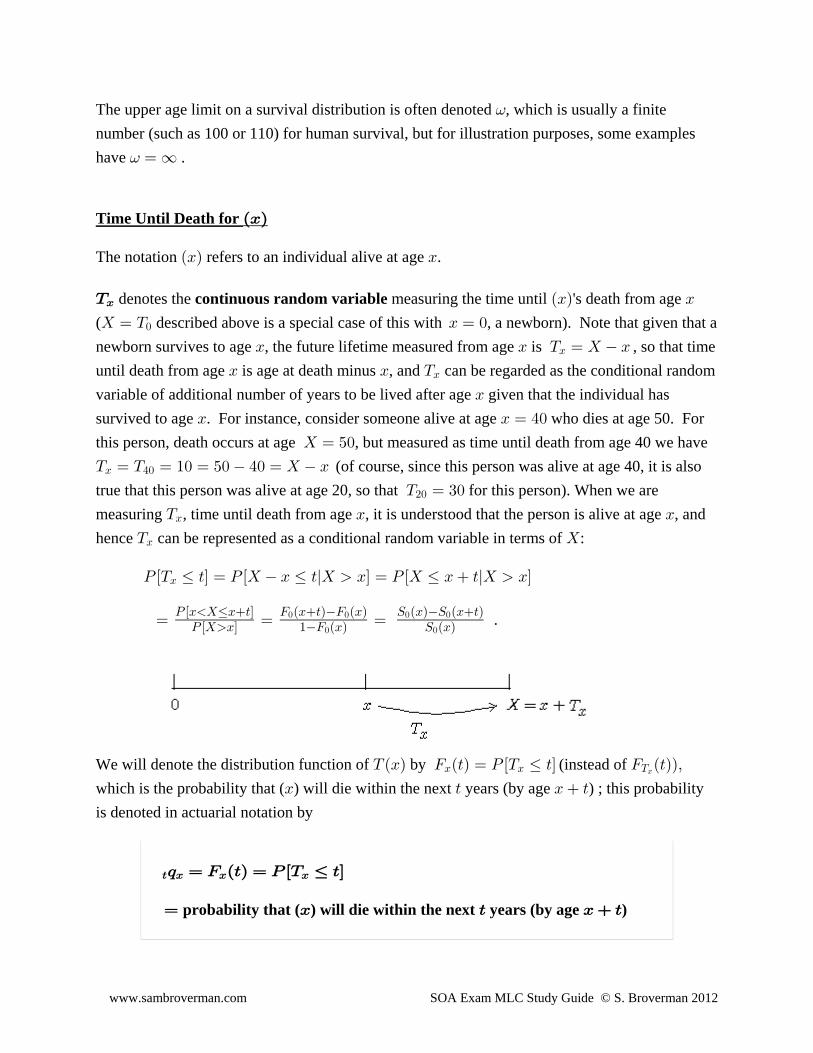
T ÒX Ÿ >Ó œ T Ò\ B Ÿ >l\ BÓ œ T Ò\ Ÿ B >l\ BÓB

.œ œ œTÒB\ŸB>Ó J ÐB>ÑJ ÐBÑ W ÐBÑW ÐB>Ñ

T Ò\BÓ "J ÐBÑ W ÐBÑ! ! ! !

! !

We will denote the distribution function of by (instead of XÐBÑ J Ð>Ñ œ T ÒX Ÿ >Ó J Ð>ÑÑßB B XB

which is the probability that ( ) will die within the next years (by age ) ; this probabilityB > B >

is denoted in actuarial notation by

> B B B; œ J Ð>Ñ œ T ÒX Ÿ >Ó

probability that ( ) will die within the next years (by age )œ B > B >


The complement of is denoted , which is> B > B; :

> B > B B: œ " ; œ T ÒX >Ó

probability that survives at least to time (and dies some time after )œ ÐBÑ > >

By the conventions of actuarial notation, for mortality or survival for a 1 year period, we write

and " B B " B B; œ ; : œ :

It is assumed that (the probability of eventually dying is 1) and∞ B; œ "

∞ B ! B: œ ! ; œ ! ß (the probability of living forever is 0). It is also assumed that . In! B: œ "

the special case that we have and .B œ ! ß \ œ XÐ!Ñ : œ =Ð>Ñ> !

Factorization of Survival Probability and Deferred Mortality Probability

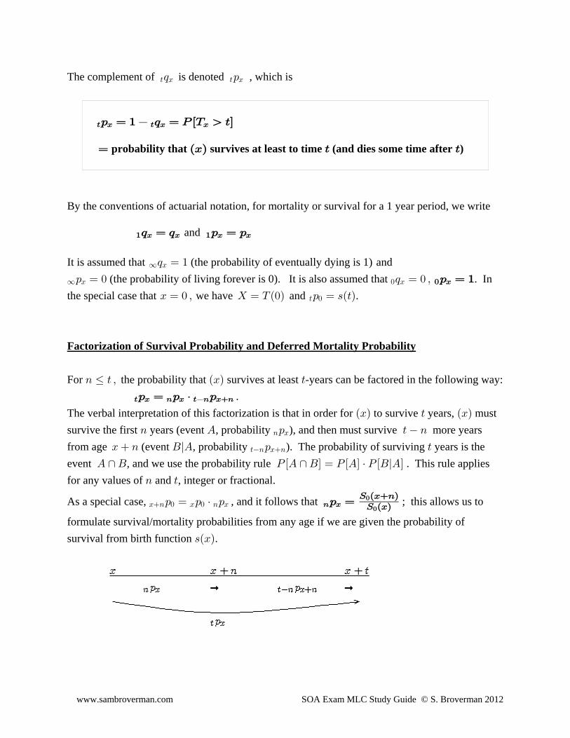
For the probability that survives at least -years can be factored in the following way:8 Ÿ > ß ÐBÑ >

> B 8 B >8 B8: œ : † : .

The verbal interpretation of this factorization is that in order for to survive years, mustÐBÑ > ÐBÑ

survive the first years (event , probability ), and then must survive more years8 E : > 88 B

from age (event , probability ). The probability of surviving years is theB 8 FlE : >>8 B8

event , and we use the probability rule . This rule appliesE ∩F T ÒE ∩ FÓ œ T ÒEÓ † T ÒFlEÓ

for any values of and , integer or fractional.8 >

As a special case, , and it follows that ; this allows us toB8 ! B ! 8 B: œ : † : 8 B: œW ÐB8ÑW ÐBÑ!

!

formulate survival/mortality probabilities from any age if we are given the probability of

survival from birth function .=ÐBÑ


If is an integer, the survival probability over the -year period can be separated into consecutive> >

one-year periods to get the factorization form .> B B B" B>": œ : † : â:

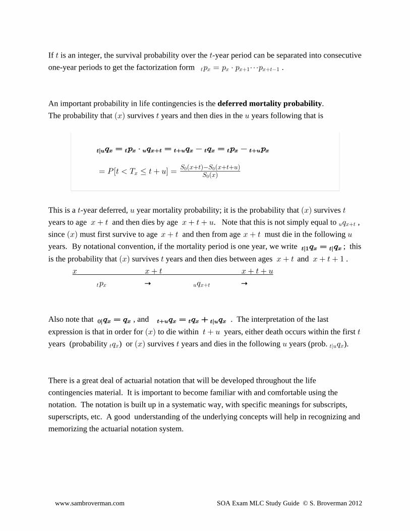
An important probability in life contingencies is the .deferred mortality probability

The probability that survives years and then dies in the years following that isÐBÑ > ?

>l? B > B ? B> >? B > B > B >? B; œ : † ; œ ; ; œ : :

œ T Ò> X Ÿ > ?Ó œBW ÐB>ÑW ÐB>?Ñ

W ÐBÑ! !

!

This is a -year deferred, year mortality probability; it is the probability that survives > ? ÐBÑ >

years to age and then dies by age . Note that this is not simply equal to ,B > B > ? ;? B>

since must first survive to age and then from age must die in the following ÐBÑ B > B > ?

years. By notational convention, if the mortality period is one year, we write ; this >l" >lB B; œ ;

is the probability that survives years and then dies between ages and .ÐBÑ > B > B > "

B B > B > ?

> B ? B>: p ; p

Also note that , and . The interpretation of the last!l >l?B B >? B > B B; œ ; ; œ ; ;

expression is that in order for to die within years, either death occurs within the first ÐBÑ > ? >

years (probability ) or survives years and dies in the following years (prob. ).> B B>l?; ÐBÑ > ? ;

There is a great deal of actuarial notation that will be developed throughout the life

contingencies material. It is important to become familiar with and comfortable using the

notation. The notation is built up in a systematic way, with specific meanings for subscripts,

superscripts, etc. A good understanding of the underlying concepts will help in recognizing and

memorizing the actuarial notation system.


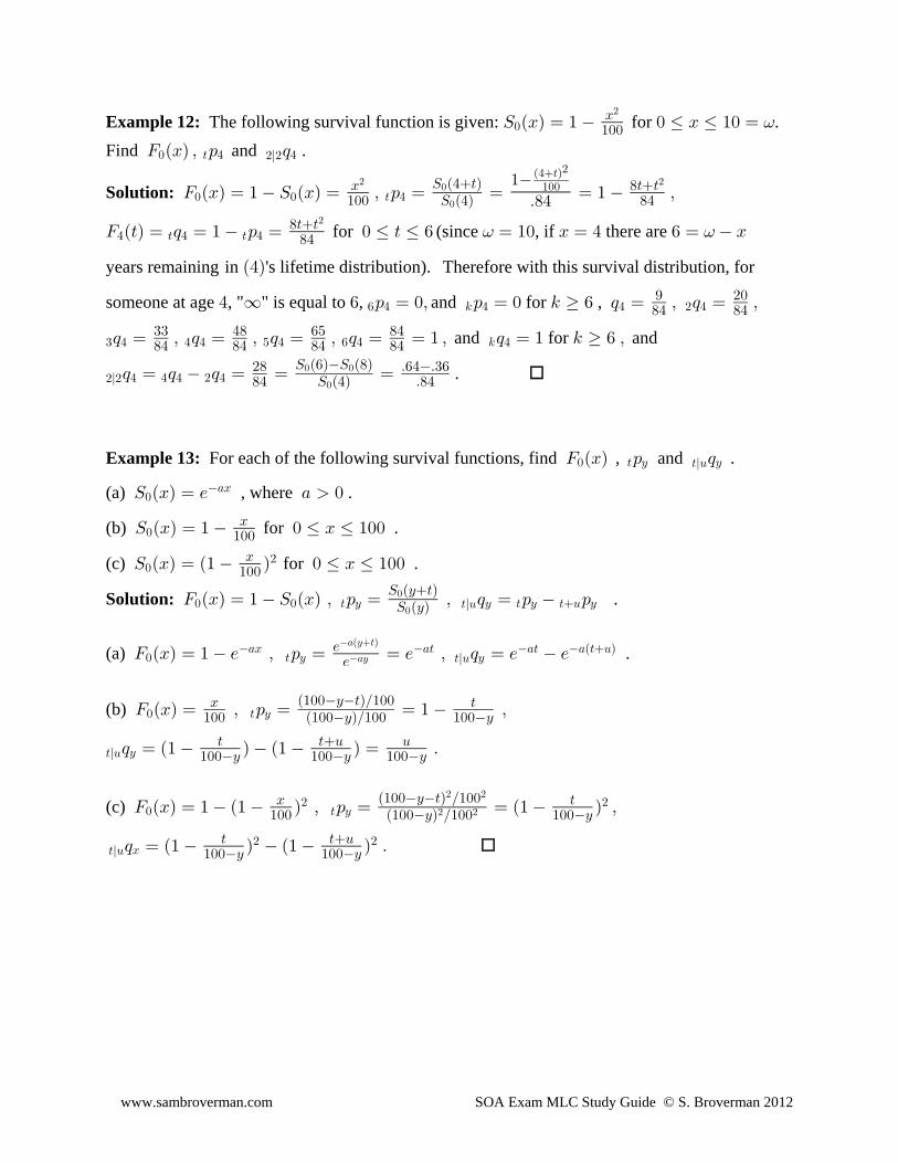
Example 12: The following survival function is given: for .W ÐBÑ œ " ! Ÿ B Ÿ "! œ!B"!!

#

=

Find and .J ÐBÑ ß : ;! > % %#l#

Solution: J ÐBÑ œ " W ÐBÑ œ ß : œ œ œ " ß! ! > %B )>>"!! W Ð%Ñ )%

W Ð%>Ñ# #!

!

"

Þ)%

Ð%>Ñ#

"!!

J Ð>Ñ œ ; œ " : œ ! Ÿ > Ÿ ' œ "! B œ % ' œ B% > % > %)>>)%

#

for (since , if there are = =

years remaining in 's lifetime distribution). Therefore with this survival distribution, forÐ%Ñ

someone at age , " " is equal to , and for , % ∞ ' : œ !ß : œ ! 5 ' ; œ ß ; œ ß' % 5 % % # %* #!)% )%

$ % % % & % ' % 5 %; œ ß ; œ ß ; œ ß ; œ œ " ß ; œ " 5 ' ß$$ %) '& )%)% )% )% )% and for and

#l# % % % # %; œ ; ; œ œ œ#) Þ'%Þ$')% W Ð%Ñ Þ)%

W Ð'ÑW Ð)Ñ! !

!.

Example 13: For each of the following survival functions, find , and .J ÐBÑ : ;! > C C>l?

(a) , where .W ÐBÑ œ / + !!+B

(b) for .W ÐBÑ œ " ! Ÿ B Ÿ "!!!B"!!

(c) for .W ÐBÑ œ Ð" Ñ ! Ÿ B Ÿ "!!!#B

"!!

Solution: .J ÐBÑ œ " W ÐBÑ ß : œ ß ; œ : :! ! > C C > C >? C>l?W ÐC>ÑW ÐCÑ!

!

(a) .J ÐBÑ œ " / ß : œ œ / ß ; œ / /! > C C+B +> +> +Ð>?Ñ

>l?//

+ÐC>Ñ

+C

(b) J ÐBÑ œ ß : œ œ " ß! > CB >"!! Ð"!!CÑÎ"!! "!!C

Ð"!!C>ÑÎ"!!

>l? C; œ Ð" Ñ Ð" Ñ œ Þ> >? ?"!!C "!!C "!!C

(c) J ÐBÑ œ " Ð" Ñ ß : œ œ Ð" Ñ ß! > C# #B >

"!! Ð"!!CÑ Î"!! "!!CÐ"!!C>Ñ Î"!!# #

# #

>l? B# #; œ Ð" Ñ Ð" Ñ Þ> >?

"!!C "!!C


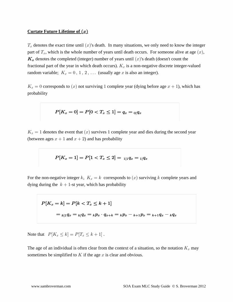
Curtate Future Lifetime of ÐBÑ

X ÐBÑB denotes the exact time until 's death. In many situations, we only need to know the integer

part of , which is the whole number of years until death occurs. For someone alive at age ,X ÐBÑB

OB denotes the completed (integer) number of years until 's death (doesn't count theÐBÑ

fractional part of the year in which death occurs). is a non-negative discrete integer-valuedOB

random variable; (usually age is also an integer).O œ ! ß " ß # ß Þ Þ Þ BB

O œ ! ÐBÑ " B "B corresponds to not surviving complete year (dying before age ), which has

probability

T ÒO œ !Ó œ T Ò! X Ÿ "Ó œ ; œ ;B B B B!l

O œ " ÐBÑB denotes the event that survives 1 complete year and dies during the second year

(between ages and ) and has probabilityB " B #

T ÒO œ "Ó œ T Ò" X Ÿ #Ó œ ; œ ;B B B B"l" "l

For the non-negative integer , corresponds to surviving complete years and5 O œ 5 ÐBÑ 5B

dying during the -st year, which has probability5 "

T ÒO œ 5Ó œ T Ò5 X Ÿ 5 "ÓB B

œ ; œ ; œ : † ; œ : : œ ; ;5l" 5lB B 5 B B5 5 B 5" B 5" B 5 B

Note that .T ÒO Ÿ 5Ó œ T ÒX Ÿ 5 "ÓB B

The age of an individual is often clear from the context of a situation, so the notation mayOB

sometimes be simplified to if the age is clear and obvious.O B


Note also, if are integers then8 >

(i) 8 B > B B B B B B B>l8> "l #l 8"l 5l5œ!

8"

; œ ; ; œ ; ; ; â ; œ ;and as a special case,

(ii) ." œ ; œ ; ; ; â œ ;∞ B B B B B"l #l 5l5œ!

∞The interpretation of (i) is that in order for to die within years, death must occur in eitherÐBÑ 8

the 1st year (prob. ), the 2nd year (prob. ), . . . , or the -th year (prob. ).; ; 8 ;B B B"l 8"l

The interpretation of (ii) is that must eventually die in some future year with probability 1.ÐBÑ

(ii) also is a verification of the probability rule for discrete random variables which states that the

sum of all individual point probabilities is 1; .5œ!

∞

T ÒO œ 5Ó œ "

A slight variation on is . is the , and it counts theO O œ O " OB B BB‡ time interval of failure

integer part of , and can be interpreted as counting the integer year, as measured from ageX OB B‡

B O O, in which death occurs. The MQR textbook tends to use , but has been the moreB‡

B

traditional curtate random variable and will be mostly used in this study guide. The difference

between the two is trivial and should not be a source of confusion or concern.

Example 12 (continued): Using for ,W ÐBÑ œ " ! Ÿ B Ÿ "! œ!B"!!

#

=

describe the probability distribution of .O%

Solution: T ÒO œ !Ó œ ; œ " : œ œ œ ß% % %W Ð%ÑW Ð&Ñ

W Ð%Ñ )%

*! !

!

)% (&"!! "!!

)%"!!

T ÒO œ "Ó œ ; œ ; ; œ : : œ œ ß% % # % % % # %"lW Ð&ÑW Ð'Ñ

W Ð%Ñ )%""! !

!

T ÒO œ #Ó œ ; œ ß T ÒO œ $Ó œ ; œ ß T ÒO œ %Ó œ ; œ ß% % % % % %#l $l %l"$ "& "()% )% )%

T ÒO œ &Ó œ ; œ T ÒO œ 'Ó œ ; œ !% % % %&l l"*)% . Note that since6

6l % ' % "! "! "!; œ : † ; œ ! † ; œ ! ;(in this survival model, is undefined since no one survives to

age ). For this probability distribution, . "! T ÒO 'Ó œ !%

Note that previous references used the notation for and for . I haveX ÐBÑ X OÐBÑ OB B

tried to update the notation in this study guide, but if you see or , they have theX ÐBÑ OÐBÑ

same meaning as and .X OB B


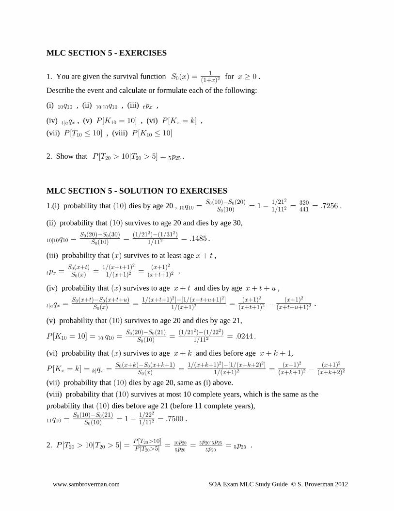
MLC SECTION 5 - EXERCISES

1. You are given the survival function for .W ÐBÑ œ B !!"

Ð"BÑ#

Describe the event and calculate or formulate each of the following:

(i) , (ii) , (iii) ,"! "! "! > B"!l"!; ; :

(iv) , (v) , (vi) ,>l? B "! B; T ÒO œ "!Ó T ÒO œ 5Ó

(vii) , (viii) T ÒX Ÿ "!Ó T ÒO Ÿ "!Ó"! "!

2. Show that .T ÒX "!lX &Ó œ :#! #! & #&

MLC SECTION 5 - SOLUTION TO EXERCISES

1.(i) probability that dies by age 20 , .Ð"!Ñ ; œ œ " œ œ Þ(#&'"! "!W Ð"!ÑW Ð#!Ñ "Î#"

W Ð"!Ñ "Î"" %%"$#!! !

!

#

#

(ii) probability that survives to age 20 and dies by age 30,Ð"!Ñ

"!l"! "!; œ œ œ Þ"%)&W Ð#!ÑW Ð$!Ñ Ð"Î#" ÑÐ"Î$" Ñ

W Ð"!Ñ "Î""! !

!

# #

# .

(iii) probability that survives to at least age ,ÐBÑ B >

> B: œ œ œW ÐB>Ñ "ÎÐB>"Ñ ÐB"ÑW ÐBÑ "ÎÐB"Ñ ÐB>"Ñ!

!

# #

# # .

(iv) probability that survives to age and dies by age ,ÐBÑ B > B > ?

>l? B; œ œ œ W ÐB>ÑW ÐB>?Ñ "ÎÐB>"Ñ ÓÒ"ÎÐB>?"Ñ Ó ÐB"Ñ ÐB"Ñ

W ÐBÑ "ÎÐB"Ñ ÐB>"Ñ ÐB>?"Ñ! !

!

# # # #

# # # .

(v) probability that survives to age 20 and dies by age 21,Ð"!Ñ

T ÒO œ "!Ó œ ; œ œ œ Þ!#%%"! "!"!lW Ð#!ÑW Ð#"Ñ Ð"Î#" ÑÐ"Î## Ñ

W Ð"!Ñ "Î""! !

!

# #

# .

(vi) probability that survives to age and dies before age ,ÐBÑ B 5 B 5 "

T ÒO œ 5Ó œ ; œ œ œ B B5lW ÐB5ÑW ÐB5"Ñ "ÎÐB5"Ñ ÓÒ"ÎÐB5#Ñ Ó ÐB"Ñ ÐB"Ñ

W ÐBÑ "ÎÐB"Ñ ÐB5"Ñ ÐB5#Ñ! !

!

# # # #

# # #

(vii) probability that dies by age 20, same as (i) above.Ð"!Ñ

(viii) probability that survives at most 10 complete years, which is the same as theÐ"!Ñ

probability that dies before age 21 (before 11 complete years),Ð"!Ñ

"" "!; œ œ " œ Þ(&!!W Ð"!ÑW Ð#"Ñ "Î##

W Ð"!Ñ "Î""! !

!

#

# .

2. .T ÒX "!lX &Ó œ œ œ œ :#! #! & #&T ÒX "!ÓT ÒX &Ó : :

: : † :#!

#! & #! & #!

"! #! & #! & #&


S. BROVERMAN MLC STUDY GUIDEPRACTICE EXAM 1

1. For a fully discrete 3-year endowment insurance of 1000 on , you are given:ÐBÑ

(i) is the prospective loss random variable at time .5P 5

(ii) (iii) 3 œ !Þ"! + œ #Þ(!")#ÞÞBÀ$l

(iv) Premiums are determined by the equivalence principle.

Calculate , given that survives to the end of the third year from issue.#P ÐBÑ

A) 540 B) 630 C) 655 D) 720 E) 910

2. For a double-decrement model:

(i) > %!wÐ"Ñ

: œ " ß ! Ÿ > Ÿ %!>"'!!

#

(ii) > %!wÐ#Ñ

: œ " ß ! Ÿ > Ÿ $!>*!!

#

Calculate ..%!#!Ð Ñ7

A) Less than .05 B) At least .05 but less than .10 C) At least .10 but less than .15

D) At least .15 but less than .20 E) At least .20

3. For independent lives (35) and (45):

(i) (ii) (iii) (iv) & $& & %& %! &!: œ !Þ*! : œ !Þ)! ; œ !Þ!$ ; œ !Þ!&

Calculate the probability that the first death of (35) and (45) occurs in the 6th year.

A) 0.0465 B) 0.0565 C) 0.0665 D) 0.0765 E) 0.0865

4. For a fully discrete whole life insurance of 100,000 on (35) you are given:

(i) Percent of premium expenses are 10% per year.

(ii) Per policy expenses are 25 per year.

(iii) Per thousand expenses are 2.50 per year.

(iv) All expenses are paid at the beginning of the year.

(v) The level annual expense loaded premium is 1234.

Calculate ."!!ß !!!T$&

A) Less than 800 B) At least 800 but less than 815 C) At least 815 but less than 830

D) At least 830 but less than 845 E) At least 845


5. A pension plan provides a retirement annuity with annual rate of:a - 2% of the first 25,000 of final year salary for each of the first 25 completed years of serviceb - 2.5% of the amount of final year salary in excess of 25,000 for each year of the first 25completed years of servicec - 3% of the first 25,000 of final year salary for each completed year of service in excess of 25yearsd - 3.5% of the amount of final salary in excess of 25,000 for each completed year of service inexcess of 25 years.If has 10 years of service already and if , then can be expressedÐ%&Ñ GEW œ $&ß !!! TEF%& '&Þ&

in the form . Find .E † F E FWW'&

%&

A) 24,000 B) 24,250 C) 24,500 D) 24,750 E) 25,000

6. is the present-value random variable for a whole life insurance of payable at the moment^ ,

of death of . You are given:ÐBÑ

(i) (ii) $ .œ !Þ!% œ !Þ!# ß > !B>

(iii) The single benefit premium for this insurance is equal to .Z +<Ð^Ñ

Calculate .,

A) 2.75 B) 3.00 C) 3.25 D) 3.50 E) 3.75

7. For a special 3-year term insurance on (30), you are given:

(i) Premiums are payable semiannually.

(ii) Premiums are payable only in the first year.

(iii) Benefits, payable at the end of the year of death, are:

5 ,5"

! "!!!

" &!!

# #&!

(iv) Mortality follows the Illustrative Life Table.

(v) Deaths are uniformly distributed within each year of age.

(vi) 3 œ !Þ!)

Calculate the amount of each semiannual benefit premium for this insurance.

A) Less than 1.2 B) At least 1.2 but less than 1.3 C) At least 1.3 but less than 1.4

D) At least 1.4 but less than 1.5 E) At least 1.5


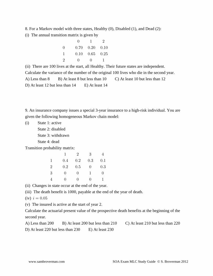
8. For a Markov model with three states, Healthy (0), Disabled (1), and Dead (2):

(i) The annual transition matrix is given by

! " #

! !Þ(! !Þ#! !Þ"!

" !Þ"! !Þ'& !Þ#&

# ! ! "

(ii) There are 100 lives at the start, all Healthy. Their future states are independent.

Calculate the variance of the number of the original 100 lives who die in the second year.



9. An insurance company issues a special 3-year insurance to a high-risk individual. You are

given the following homogeneous Markov chain model:

(i) State 1: active

State 2: disabled

State 3: withdrawn

State 4: dead

Transition probability matrix:

" # $ %

" !Þ% !Þ# !Þ$ !Þ"

# !Þ# !Þ& ! !Þ$

$ ! ! " !

% ! ! ! "

(ii) Changes in state occur at the end of the year.

(iii) The death benefit is 1000, payable at the end of the year of death.

(iv) 3 œ !Þ!&

(v) The insured is active at the start of year 2.

Calculate the actuarial present value of the prospective death benefits at the beginning of the

second year.




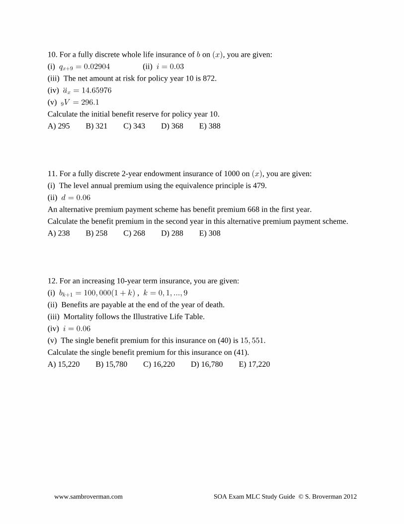
10. For a fully discrete whole life insurance of on , you are given:, ÐBÑ

(i) (ii) ; œ !Þ!#*!% 3 œ !Þ!$B*

(iii) The net amount at risk for policy year 10 is 872.

(iv) + œ "%Þ'&*('ÞÞB

(v) *Z œ #*'Þ"

Calculate the initial benefit reserve for policy year 10.

A) 295 B) 321 C) 343 D) 368 E) 388

11. For a fully discrete 2-year endowment insurance of 1000 on , you are given:ÐBÑ

(i) The level annual premium using the equivalence principle is 479.

(ii) . œ !Þ!'

An alternative premium payment scheme has benefit premium 668 in the first year.

Calculate the benefit premium in the second year in this alternative premium payment scheme.

A) 238 B) 258 C) 268 D) 288 E) 308

12. For an increasing 10-year term insurance, you are given:

(i) , , œ "!!ß !!!Ð" 5Ñ 5 œ !ß "ß ÞÞÞß *5"

(ii) Benefits are payable at the end of the year of death.

(iii) Mortality follows the Illustrative Life Table.

(iv) 3 œ !Þ!'

(v) The single benefit premium for this insurance on (40) is ."&ß &&"

Calculate the single benefit premium for this insurance on (41).

A) 15,220 B) 15,780 C) 16,220 D) 16,780 E) 17,220


13. For a fully discrete whole life insurance of 1000 on :ÐBÑ

(i) Death is the only decrement.

(ii) The annual benefit premium is 80.

(iii) Expenses in year 1, payable at the start of the year, are 40% of contract premiums.

(iv) The starting asset share is 0 and the asset share at the end of the first year is 16.84.

(v) (vi) 3 œ !Þ"! "!!! Z œ %!" B

Calculate the level annual contract premium.

A) 100 B) 102 C) 104 D) 106 E) 108

14. You are given:

(i) is the future lifetime random variable for .X ÐBÑB

(ii) W œ " ß ! Ÿ B ŸBB= =

(iii) Z +<ÐX Ñ œ $&#Þ"$!

Calculate °/$!À%!lA) 26.7 B) 27.7 C) 28.7 D) 29.7 E) 30.7

15. A fully discrete 3-year term insurance of 10,000 on (40) is based on a double-decrement

model, death and withdrawal:

(i) Decrement 1 is death. (ii) ; œ !Þ!# ß 5 !B5Ð"Ñ

(iii) Decrement 2 is withdrawal, which occurs at the end of the year.

(iv) , (v) ; œ !Þ!% 5 œ !ß "ß # @ œ !Þ*&%!5wÐ#Ñ

Calculate the actuarial present value of the death benefits for this insurance.

A) 492 B) 502 C) 512 D) 522 E) 532

16. For a fully discrete 5-payment 10-year decreasing term insurance on (60), you are given:

(i) , œ "!!!Ð"! 5Ñ ß 5 œ !ß "ß #ß ÞÞÞß *5"

(ii) ; œ !Þ!# !Þ!!"5 ß 5 œ !ß "ß #ß ÞÞÞß *'!5

(iii) 3 œ !Þ!'

(iv) The benefit reserve at the end of year 2 is .#Z œ ((Þ''

Calculate the level annual benefit premium.

A) 188 B) 194 C) 202 D) 210 E) 218


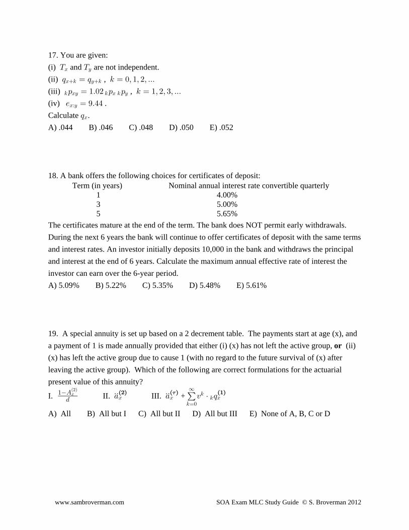
17. You are given:

(i) and are not independent.X XB C

(ii) , ; œ ; 5 œ !ß "ß #ß ÞÞÞB5 C5

(iii) , 5 BC 5 B 5 C: œ "Þ!# : : 5 œ "ß #ß $ß ÞÞÞ

(iv) ./ œ *Þ%%BÀC

Calculate .;B

A) .044 B) .046 C) .048 D) .050 E) .052

18. A bank offers the following choices for certificates of deposit: Term (in years) Nominal annual interest rate convertible quarterly 1 4.00% 3 5.00% 5 5.65%

The certificates mature at the end of the term. The bank does NOT permit early withdrawals.

During the next 6 years the bank will continue to offer certificates of deposit with the same terms

and interest rates. An investor initially deposits 10,000 in the bank and withdraws the principal

and interest at the end of 6 years. Calculate the maximum annual effective rate of interest the

investor can earn over the 6-year period.

A) 5.09% B) 5.22% C) 5.35% D) 5.48% E) 5.61%

19. A special annuity is set up based on a 2 decrement table. The payments start at age (x), and

a payment of 1 is made annually provided that either (i) (x) has not left the active group, (ii)or

(x) has left the active group due to cause 1 (with no regard to the future survival of (x) after

leaving the active group). Which of the following are correct formulations for the actuarial

present value of this annuity?

I. II. III. + "E.

BÐ#Ñ

+ + @ † ;ÞÞ ÞÞB B B

5œ!

∞5

5Ð#Ñ Ð Ñ Ð"Ñ7

A) All B) All but I C) All but II D) All but III E) None of A, B, C or D


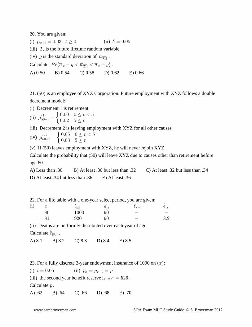
20. You are given:

(i) (ii) . $B> œ !Þ!$ ß > ! œ !Þ!&

(iii) is the future lifetime random variable. XB

(iv) is the standard deviation of .1 +X lB

Calculate .T< + 1 + + 1 B BX lB

A) 0.50 B) 0.54 C) 0.58 D) 0.62 E) 0.66

21. (50) is an employee of XYZ Corporation. Future employment with XYZ follows a double

decrement model:

(i) Decrement 1 is retirement

(ii) .&!>Ð"Ñ

œ!Þ!! ! Ÿ > &!Þ!# & Ÿ >

(iii) Decrement 2 is leaving employment with XYZ for all other causes

(iv) .&!>Ð#Ñ

œ!Þ!& ! Ÿ > &!Þ!$ & Ÿ >

(v) If (50) leaves employment with XYZ, he will never rejoin XYZ.

Calculate the probability that (50) will leave XYZ due to causes other than retirement before

age 60.



22. For a life table with a one-year select period, you are given:(i) °B j . j /ÒBÓ ÒBÓ ÒBÓB"

)! "!!! *! )" *#! *! )Þ#

(ii) Deaths are uniformly distributed over each year of age.

Calculate .°/Ò)!ÓA) 8.1 B) 8.2 C) 8.3 D) 8.4 E) 8.5

23. For a fully discrete 3-year endowment insurance of 1000 on :ÐBÑ

(i) (ii) 3 œ !Þ!& : œ : œ :B B"

(iii) the second year benefit reserve is .#Z œ &#'

Calculate .:

A) .62 B) .64 C) .66 D) .68 E) .70


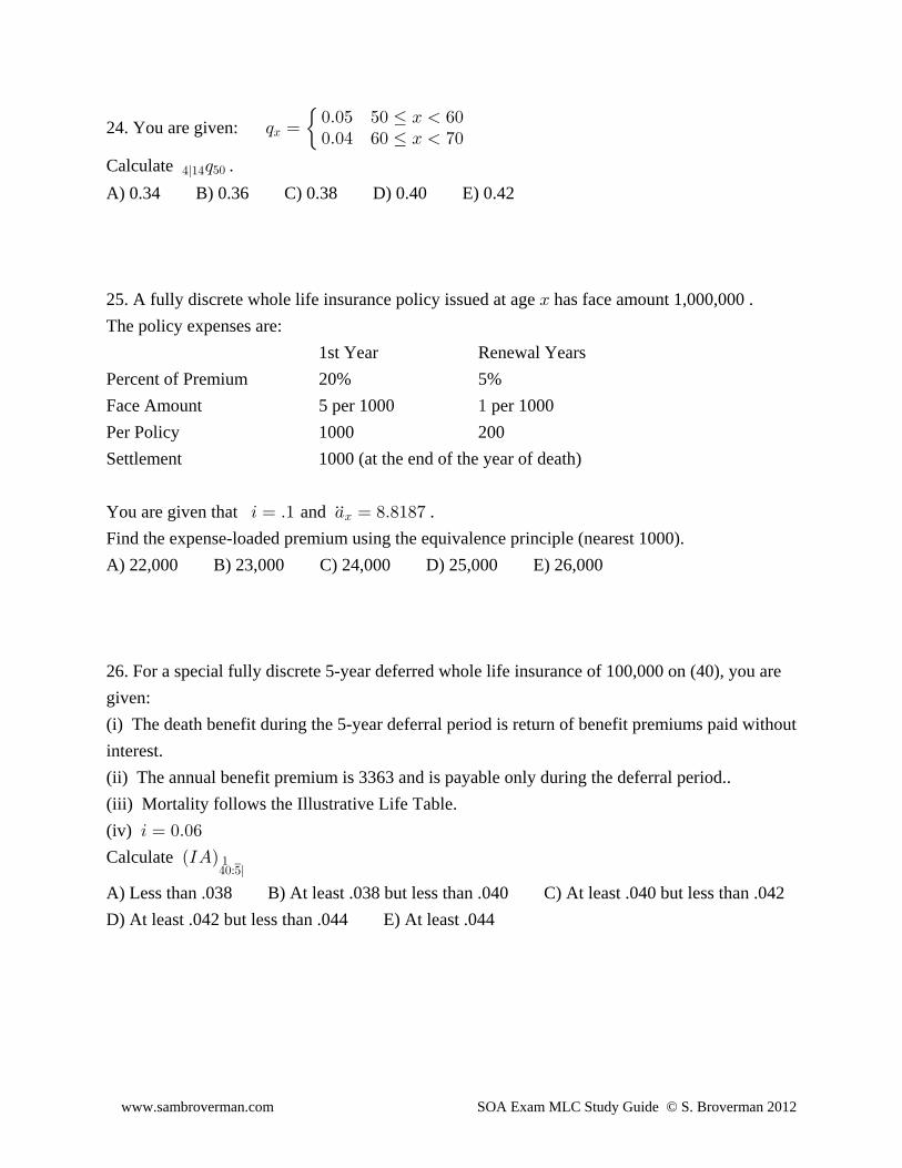
24. You are given: ; œ!Þ!& &! Ÿ B '!!Þ!% '! Ÿ B (!B

Calculate .%l"% &!;

A) 0.34 B) 0.36 C) 0.38 D) 0.40 E) 0.42

25. A fully discrete whole life insurance policy issued at age has face amount 1,000,000 .B

The policy expenses are:

1st Year Renewal Years

Percent of Premium 20% 5%

Face Amount 5 per 1000 per 1000"

Per Policy 1000 200

Settlement 1000 (at the end of the year of death)

You are given that and .3 œ Þ" + œ )Þ)")(ÞÞB

Find the expense-loaded premium using the equivalence principle (nearest 1000).

A) 22,000 B) 23,000 C) 24,000 D) 25,000 E) 26,000

26. For a special fully discrete 5-year deferred whole life insurance of 100,000 on (40), you are

given:

(i) The death benefit during the 5-year deferral period is return of benefit premiums paid without

interest.

(ii) The annual benefit premium is 3363 and is payable only during the deferral period..

(iii) Mortality follows the Illustrative Life Table.

(iv) 3 œ !Þ!'

Calculate ÐMEÑ%!À&l"




27. You are pricing a special 3-year annuity-due on two independent lives, and . The B ÐCÑ

annuity pays 30,000 if both persons are alive 20,000 if dies first and 10,000 if dies first.ß ÐBÑ ÐCÑ

You are given:

(i) 5 : œ :5 B 5 C

" !Þ*"

# !Þ)#

$ !Þ(#

(ii) 3 œ !Þ!&

Calculate the actuarial present value of this annuity (nearest 100).

A) 78,300 B) 80,400 C) 82,500 D) 84,700 E) 86,800

28. Company ABC sets the contract premium for a continuous life annuity of 1 per year on ÐBÑ

equal to the single benefit premium calculated using:

(i) (ii) for for

$ .œ !Þ!$ œ!Þ!# > Ÿ "!!Þ!" > "!B>

However, a revised mortality assumption reflects future mortality improvement and is given by

.B> œ !Þ!# ß > !

Calculate the expected gain at issue for ABC (using the revised mortality assumption) as a

percentage of the contract premium.

A) 2% B) 8% C) 13% D) 18% E) 23%

29. A fully continuous whole life insurance of face amount 1 is based on the following

assumptions:

• constant force of interest of 6%

• constant force of mortality of .015 at all ages

• annual contract premium of .016

An insurer determines that with a portfolio of independent policies of this type, using the8

normal approximation, the probability of a positive loss on all policies combined is .05. How

many additional independent policies of the same type would be needed to reduce the probability

of a positive total loss to .025 (continuing to use the normal approximation)?

A) Less than 500 B) At least 500, but less than 600 C) At least 600, but less than 700

D) At least 700, but less than 800 E) At least 800


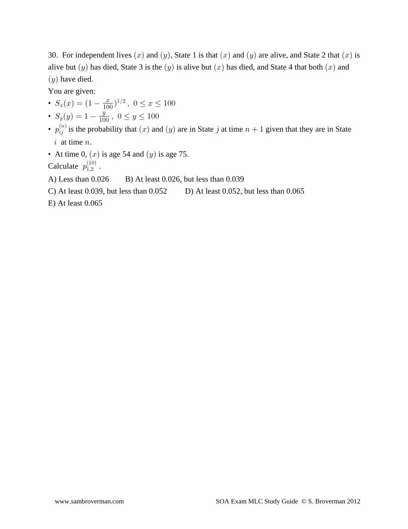
30. For independent lives and , State 1 is that and are alive, and State 2 that isÐBÑ ÐCÑ ÐBÑ ÐCÑ ÐBÑ

alive but has died, State 3 is the is alive but has died, and State 4 that both andÐCÑ ÐCÑ ÐBÑ ÐBÑ

ÐCÑ have died.

You are given:

• W ÐBÑ œ Ð" Ñ ß ! Ÿ B Ÿ "!!B"Î#B

"!!

• W ÐCÑ œ " ß ! Ÿ C Ÿ "!!CC

"!!

• is the probability that and are in State at time given that they are in State: ÐBÑ ÐCÑ 4 8 "34Ð8Ñ

at time .3 8

• At time 0, is age 54 and is age 75.ÐBÑ ÐCÑ

Calculate .:"ß#Ð"!Ñ

A) Less than 0.026 B) At least 0.026, but less than 0.039

C) At least 0.039, but less than 0.052 D) At least 0.052, but less than 0.065

E) At least 0.065


S. BROVERMAN MLC STUDY GUIDEPRACTICE EXAM 1 SOLUTIONS

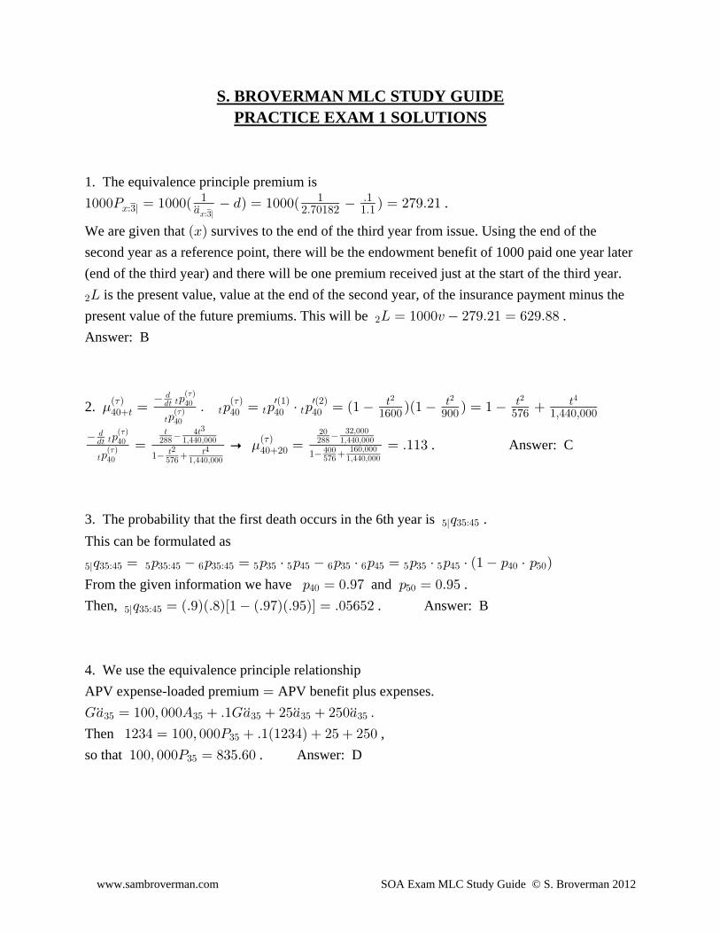
1. The equivalence principle premium is

"!!!T œ "!!!Ð .Ñ œ "!!!Ð Ñ œ #(*Þ#"BÀ$l" " Þ"

+ #Þ(!")# "Þ"ÞÞBÀ$l

.

We are given that survives to the end of the third year from issue. Using the end of theÐBÑ

second year as a reference point, there will be the endowment benefit of 1000 paid one year later

(end of the third year) and there will be one premium received just at the start of the third year.

#P is the present value, value at the end of the second year, of the insurance payment minus the

present value of the future premiums. This will be . #P œ "!!!@ #(*Þ#" œ '#*Þ))

Answer: B

2. .%!> %! %! %!Ð Ñ Ð Ñ wÐ"Ñ wÐ#Ñ

> > >7 7

œ Þ : œ : † : œ Ð" ÑÐ" Ñ œ " :

:

> > > >"'!! *!! &(' "ß%%!ß!!!

..> > %!

Ð Ñ

> %!Ð Ñ

# # # %7

7

:

:

..> > %!

Ð Ñ

> %!Ð Ñ %!!

> %> #!#)) "ß%%!ß!!! #)) "ß%%!ß!!!

$

> ># %

&(' "ß%%!ß!!!

$#ß!!!

&(' "ß%%!ß!!!"'!ß!!!

7

7 œ p œ œ Þ""$

" %!#!Ð Ñ

" . Answer.

7 : C

3. The probability that the first death occurs in the 6th year is .&l $&À%&;

This can be formulated as

&l $&À%& & $&À%& ' $&À%& & $& & %& ' $& ' %& & $& & %& %! &!; œ : : œ : † : : † : œ : † : † Ð" : † : Ñ

From the given information we have and .: œ !Þ*( : œ !Þ*&%! &!

Then, . Answer: B&l $&À%&; œ ÐÞ*ÑÐÞ)ÑÒ" ÐÞ*(ÑÐÞ*&ÑÓ œ Þ!&'&#

4. We use the equivalence principle relationship

APV expense-loaded premium APV benefit plus expenses.œ

K+ œ "!!ß !!!E Þ"K+ #&+ #&!+ ÞÞÞ ÞÞ ÞÞ ÞÞ$& $& $& $& $&

Then ,"#$% œ "!!ß !!!T Þ"Ð"#$%Ñ #& #&!$&

so that . Answer: D"!!ß !!!T œ )$&Þ'!$&


5. TEF œ'&Þ& (.02)(25,000)(25) + (.025) 35,000 25,000 (25) SS

65

45

+ (.03)(25,000)(5) + (.035) 35,000 25,000 (5) = 3750 + 28,000 SS

65

45 S

S65

45

. Answer: B.p E F œ #%ß #&!

6. The variance of the continuous whole life insurance with face amount is,

Z +<Ò^Ó œ , Ò E ÐE Ñ Ó œ Þ!% # # #

B B . Since the force of mortality is constant at .02 and ,$

E œ œ œ E œ œ œ

B B#. .

$ . $ . !%!# $ # Þ!)!# &Þ!# " Þ!# "

. and , so that

Z +<Ò^Ó œ , Ò Ð Ñ Ó œ ,E œ , †# #

B" " %, "& $ %& $

#

. The single benefit premium is . We are told that

, † œ , œ $Þ(&" %,$ %&

#

, from which we get . Answer: E

7. We assume that we are to find premiums based on the equivalence principle.

We will denote each of the two premiums as (assume to be paid the start of each half-yearU

during the first year). The APV of the premiums is .UÒ" @ † : ÓÞ&Þ& $!

The APV of the benefit is ."!!!@; &!!@ ; #&!@ ;$! $! $!# $"l #l

From the Illustrative Table, we have and .; œ Þ!!"&$ ß ; œ Þ!!"'" ; œ Þ!!"(!$! $" $#

Using UDD, the APV of premiums is .UÒ" @ Ð" Þ&ÐÞ!!"&$ÑÑÓ œ "Þ*'"&"%UÞ&

The APV of the benefit is

"!!!@ÐÞ!!"&$Ñ &!!@ ÐÞ**)%(ÑÐÞ!!"'"Ñ #&!@ ÐÞ**)%(ÑÐÞ**)$*ÑÐÞ!!"(!Ñ œ #Þ%%#!)* Þ# $

Then . Answer: EU œ œ "Þ#%&#Þ%%#!)*"Þ*'"&"%

8. Let denote the probability of dying during the second year. Then the number of deaths in; R

the second year has a binomial distribution based on trials and success (dying)7 œ "!!

probability . The variance of the binomial is .; Z +<ÒRÓ œ 7;Ð" ;Ñ œ "!!;Ð" ;Ñ

; ; œ T Ò Ó can be formulated as survive 1st year and die in 2nd year , which is equal to

œ U † U U † U œ ÐÞ(ÑÐÞ"Ñ ÐÞ#ÑÐÞ#&Ñ œ Þ"#Ð!ß!Ñ Ð!ß#Ñ Ð!ß"Ñ Ð"ß#Ñ

(this is the combination of staying healthy for the 1st year and dying in the 2nd year, or

becoming disabled in the 1st year and dying in the 2nd year).

Therefore . Answer: CZ +<ÒRÓ œ "!!ÐÞ"#ÑÐÞ))Ñ œ "!Þ&'


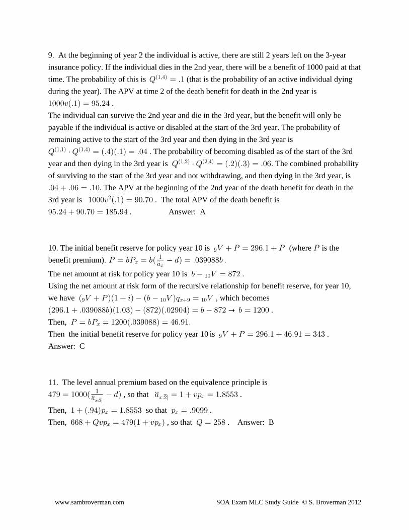
9. At the beginning of year 2 the individual is active, there are still 2 years left on the 3-year

insurance policy. If the individual dies in the 2nd year, there will be a benefit of 1000 paid at that

time. The probability of this is (that is the probability of an active individual dyingU œ Þ"Ð"ß%Ñ

during the year). The APV at time 2 of the death benefit for death in the 2nd year is

"!!!@ÐÞ"Ñ œ *&Þ#% .

The individual can survive the 2nd year and die in the 3rd year, but the benefit will only be

payable if the individual is active or disabled at the start of the 3rd year. The probability of

remaining active to the start of the 3rd year and then dying in the 3rd year is

U † U œ ÐÞ%ÑÐÞ"Ñ œ Þ!%Ð"ß"Ñ Ð"ß%Ñ . The probability of becoming disabled as of the start of the 3rd

year and then dying in the 3rd year is The combined probabilityU † U œ ÐÞ#ÑÐÞ$Ñ œ Þ!'ÞÐ"ß#Ñ Ð#ß%Ñ

of surviving to the start of the 3rd year and not withdrawing, and then dying in the 3rd year, is

Þ!% Þ!' œ Þ"!. The APV at the beginning of the 2nd year of the death benefit for death in the

3rd year is . The total APV of the death benefit is"!!!@ ÐÞ"Ñ œ *!Þ(!#

*&Þ#% *!Þ(! œ ")&Þ*% . Answer: A

10. The initial benefit reserve for policy year 10 is (where is the*Z T œ #*'Þ" T T

benefit premium). T œ ,T œ ,Ð .Ñ œ Þ!$*!)), ÞB"+ÞÞB

The net amount at risk for policy year 10 is ., Z œ )(#"!

Using the net amount at risk form of the recursive relationship for benefit reserve, for year 10,

we have , which becomesÐ Z TÑÐ" 3Ñ Ð, Z Ñ; œ Z* "! B* "!

Ð#*'Þ" Þ!$*!)),ÑÐ"Þ!$Ñ Ð)(#ÑÐÞ!#*!%Ñ œ , )(# p , œ "#!! .

Then, T œ ,T œ "#!!ÐÞ!$*!))Ñ œ %'Þ*"ÞB

Then the initial benefit reserve for policy year 10 is . *Z T œ #*'Þ" %'Þ*" œ $%$

Answer: C

11. The level annual premium based on the equivalence principle is

%(* œ "!!!Ð .Ñ + œ " @: œ "Þ)&&$ÞÞ"

+ÞÞBÀ#l

, so that .BÀ#l B

Then, so that ." ÐÞ*%Ñ: œ "Þ)&&$ : œ Þ*!**B B

Then, , so that . Answer: B'') U@: œ %(*Ð" @: Ñ U œ #&)B B


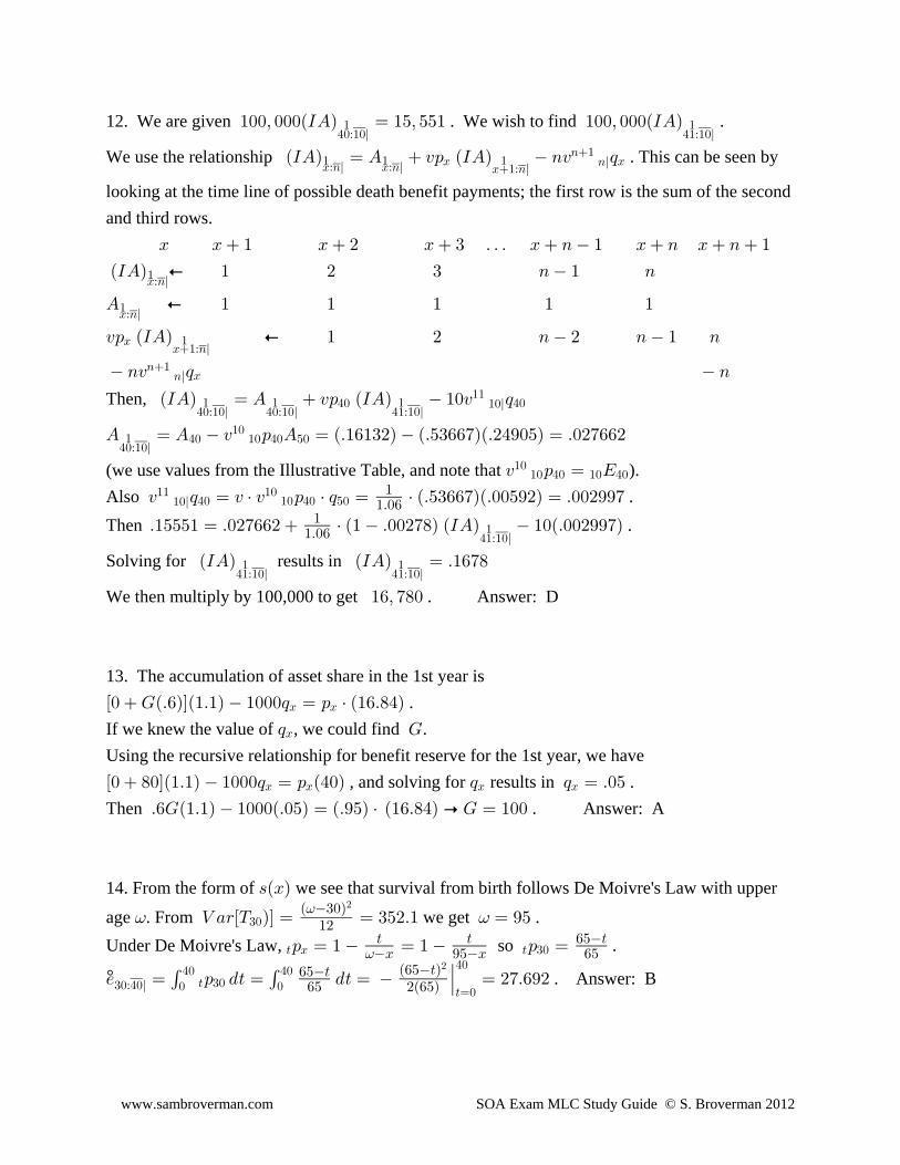
12. We are given . We wish to find ."!!ß !!!ÐMEÑ œ "&ß &&" "!!ß !!!ÐMEÑ%!À"!l %"À"!l" "

We use the relationship . This can be seen byÐMEÑ œ E @: ÐMEÑ 8@ ;BÀ8l BÀ8l" " "B B

B"À8l

8"8l

looking at the time line of possible death benefit payments; the first row is the sum of the second

and third rows.

B B " B # B $ Þ Þ Þ B 8 " B 8 B 8 "

ÐMEÑ o " # $ 8 " 8BÀ8l"

E o " " " " "BÀ8l"

@: ÐMEÑ o " # 8 # 8 " 8BB"À8l"

8@ ; 88"8l B

Then, ÐMEÑ œ E @: ÐMEÑ "!@ ;%!À"!l %!À"!l %"À"!l" " "%! %!

"""!l

E œ E @ : E œ ÐÞ"'"$#Ñ ÐÞ&$''(ÑÐÞ#%*!&Ñ œ Þ!#(''#%!À"!l" %! "! %! &!

"!

(we use values from the Illustrative Table, and note that ).@ : œ I"!"! %! "! %!

Also .@ ; œ @ † @ : † ; œ † ÐÞ&$''(ÑÐÞ!!&*#Ñ œ Þ!!#**("" "!"!l %! "! %! &!

""Þ!'

Then .Þ"&&&" œ Þ!#(''# † Ð" Þ!!#()Ñ ÐMEÑ "!ÐÞ!!#**(Ñ""Þ!' %"À"!l

"

Solving for results in ÐMEÑ ÐMEÑ œ Þ"'()%"À"!l %"À"!l" "

We then multiply by 100,000 to get . Answer: D"'ß ()!

13. The accumulation of asset share in the 1st year is

Ò! KÐÞ'ÑÓÐ"Þ"Ñ "!!!; œ : † Ð"'Þ)%ÑB B .

If we knew the value of , we could find .; KB

Using the recursive relationship for benefit reserve for the 1st year, we have

Ò! )!ÓÐ"Þ"Ñ "!!!; œ : Ð%!Ñ ; ; œ Þ!&B B B B , and solving for results in .

Then . Answer: AÞ'KÐ"Þ"Ñ "!!!ÐÞ!&Ñ œ ÐÞ*&Ñ † Ð"'Þ)%Ñ p K œ "!!

14. From the form of we see that survival from birth follows De Moivre's Law with upper=ÐBÑ

age . From we get .= =Z +<ÒX ÑÓ œ œ $&#Þ" œ *&$!Ð $!Ñ

"#= #

Under De Moivre's Law, so .> B > $!: œ " œ " : œ> > '&>B *&B '&=

/ œ : .> œ .> œ œ #(Þ'*#° . Answer: B$!À%!l ! !%! %!

> $!>œ!

%! '&>'& #Ð'&Ñ

Ð'&>Ñ#


15. The APV of the death benefit is ."!ß !!!Ò@; @ ; @ ; Ó%! %! %!Ð"Ñ Ð"Ñ Ð"Ñ# $

"l #l

Since decrement 2 occurs at the end of the year, for each year, , and; œ ;B BÐ"Ñ wÐ"Ñ

; œ Ð" ; Ñ † ;B B BÐ#Ñ wÐ"Ñ wÐ#Ñ .

For decrement 1, we have for , since the force of decrement is; œ ; œ Þ!# B œ %!ß %"ß %#B BÐ"Ñ wÐ"Ñ

constant. Also for .: œ : † : œ ÐÞ*)Ñ † ÐÞ*'Ñ œ Þ*%!) B œ %!ß %"B B BÐ Ñ wÐ"Ñ wÐ#Ñ7

Then, and"l %! %! %"Ð"Ñ Ð Ñ Ð"Ñ

; œ : † ; œ ÐÞ*%!)ÑÐÞ!#Ñ œ Þ!"))"'7

#l %! %! %# %! %" %#Ð"Ñ Ð Ñ Ð"Ñ Ð Ñ Ð Ñ Ð"Ñ

##; œ : † ; œ : † : † ; œ ÐÞ*%!)Ñ ÐÞ!#Ñ œ Þ!"((!

7 7 7 .

The APV of the death benefit is

"!ß !!!Ò@ÐÞ!#Ñ @ ÐÞ!"))"'Ñ @ ÐÞ!"((!ÑÓ œ &"## $ . Answer: C

16. We use the recursive reserve formula, .Ð Z TÑÐ" 3Ñ , † ; œ : † Z5 5" B5 B5 5"

Also, for benefit reserves. For the first year, we have!Z œ !

Ð! TÑÐ"Þ!'Ñ "!ß !!!ÐÞ!#Ñ œ Þ*) † Z p Z œ "Þ!)"'T #!%Þ!)" " .

For the second year, we have

Ð"Þ!)"'T #!%Þ!) TÑÐ"Þ!'Ñ *ß !!!ÐÞ!#"Ñ œ Þ*(* † Z œ ÐÞ*(*ÑÐ((Þ''Ñ œ ('Þ!$#

. Answer: Ep T œ #")

17. is a valid relationship for all survival distributions of and ,/ œ / / / XÐBÑ X ÐCÑBC B C BC

whether or not they are independent. Since for all , it follows that for; œ Þ!& 5 : œ Þ*&B5 B5

all , and then . This follows from the fact that5 / œ : œ Ð: Ñ œB > B B>œ" >œ"

∞ ∞> :

":B

B

> B B B" B>"> # $: œ : † : â: œ ÐÞ*&Ñ " < < < â œ and ."

"<

Also, , since for all ./ œ ; œ ; 5C B5 C5:

":B

B

/ œ : œ "Þ!#Ð: Ñ œ "Þ!# † œ *Þ%%BC > BC B>œ" >œ"

∞ ∞#> Ð: Ñ

"Ð: ÑB

#

B# .

Then , and and . Answer: D: œ Þ*!#& : œ Þ*& ; œ Þ!&B#

B B


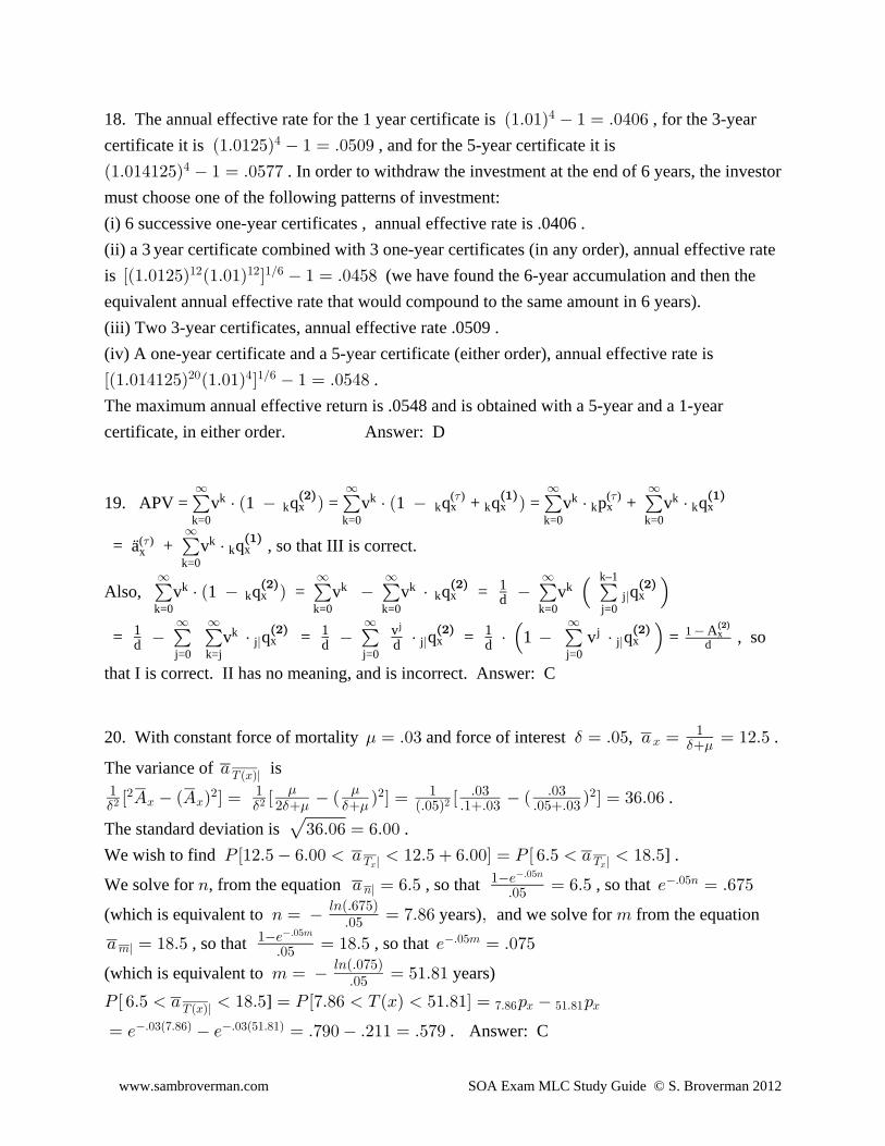
18. The annual effective rate for the 1 year certificate is , for the 3-yearÐ"Þ!"Ñ " œ Þ!%!'%

certificate it is , and for the 5-year certificate it isÐ"Þ!"#&Ñ " œ Þ!&!*%

Ð"Þ!"%"#&Ñ " œ Þ!&((% . In order to withdraw the investment at the end of 6 years, the investor

must choose one of the following patterns of investment:

(i) 6 successive one-year certificates , annual effective rate is .0406 .

(ii) a 3 year certificate combined with 3 one-year certificates (in any order), annual effective rate

is (we have found the 6-year accumulation and then theÒÐ"Þ!"#&Ñ Ð"Þ!"Ñ Ó " œ Þ!%&)"# "# "Î'

equivalent annual effective rate that would compound to the same amount in 6 years).

(iii) Two 3-year certificates, annual effective rate .0509 .

(iv) A one-year certificate and a 5-year certificate (either order), annual effective rate is

ÒÐ"Þ!"%"#&Ñ Ð"Þ!"Ñ Ó " œ Þ!&%)#! % "Î' .

The maximum annual effective return is .0548 and is obtained with a 5-year and a 1-year

certificate, in either order. Answer: D

19. APV = v 1 q = v 1 q + q = v p + v q k=0 k=0 k=0 k=0

k k k kk k k k kx x x x x

( ) ( )∞ ∞ ∞ ∞

† Ð Ñ † Ð Ñ † †Ð#Ñ Ð"Ñ Ð"Ñ7 7

= a + v q , so that III is correct.¨( )x

k=0

kk x

7 ∞ †Ð"Ñ

Also, v 1 q = v v q = v q k=0 k=0 k=0 k=0 j=0

k k k kk kx x x

k–1

j

∞ ∞ ∞ ∞

±† Ð Ñ † Ð#Ñ Ð#Ñ Ð#Ñ 1

d

= v q = q = 1 v q = , so1 1 v 1d d d d

A † † † † j=0 k=j j=0 j=0

k jj j jx x x

1d

∞ ∞ ∞ ∞

± ± ±Ð#Ñ Ð#Ñ Ð#Ñ

jx Ð#Ñ

that I is correct. II has no meaning, and is incorrect. Answer: C

20. With constant force of mortality and force of interest , .. $œ Þ!$ œ Þ!& + œ œ "#Þ&B

"$ .

The variance of is+XÐBÑl

" " " Þ!$ Þ!$# ÐÞ!&Ñ Þ"Þ!$ Þ!&Þ!$$ $ $ . $ .. .

# # #Ò E ÐE Ñ Ó œ Ò Ð Ñ Ó œ Ò Ð Ñ Ó œ $'Þ!' # # # #

B B .

The standard deviation is .$'Þ!' œ 'Þ!!

We wish to find ] .T Ò"#Þ& 'Þ!! + "#Þ& 'Þ!!Ó œ T Ò 'Þ& + ")Þ& X l X lB B

We solve for , from the equation , so that , so that 8 + œ 'Þ& œ 'Þ& / œ Þ'(&8l

Þ!&8"/Þ!&

Þ!&8

(which is equivalent to years) and we solve for from the equation8 œ œ (Þ)' ß 768ÐÞ'(&Ñ

Þ!&

+ œ ")Þ& œ ")Þ& / œ Þ!(&7l

Þ!&7 , so that , so that "/Þ!&

Þ!&7

(which is equivalent to years)7 œ œ &"Þ)"68ÐÞ!(&Ñ

Þ!&

T Ò 'Þ& + ")Þ& œ T Ò(Þ)' XÐBÑ &"Þ)"Ó œ : :XÐBÑl (Þ)' B &"Þ)" B]

œ / / œ Þ(*! Þ#"" œ Þ&(*Þ!$Ð(Þ)'Ñ Þ!$Ð&"Þ)"Ñ . Answer: C


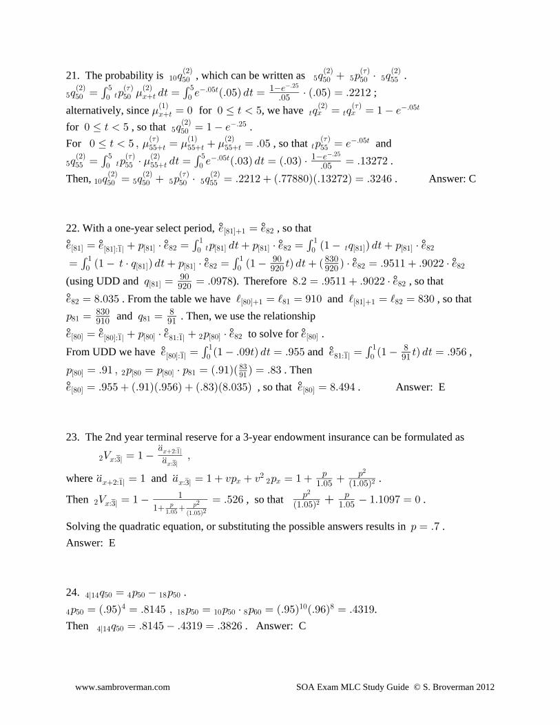
21. The probability is , which can be written as ."! & & &&! &! &! &&Ð#Ñ Ð#Ñ Ð Ñ Ð#Ñ

; ; : † ;7

& >&! &!Ð#Ñ Ð Ñ Ð#Ñ

! !& &

B>Þ!&>; œ : .> œ / ÐÞ!&Ñ .> œ † ÐÞ!&Ñ œ Þ##"# 7

. "/Þ!&

Þ#&

;

alternatively, since for , we have .B>Ð"Ñ Ð#Ñ Ð Ñ

> >B BÞ!&>œ ! ! Ÿ > & ; œ ; œ " /

7

for , so that .! Ÿ > & ; œ " /& &!Ð#Ñ Þ#&

For , so that and! Ÿ > & ß œ œ Þ!& : œ /. . .&&> &&> &&> &&Ð Ñ Ð"Ñ Ð#Ñ Ð Ñ

>Þ!&>7 7

& >&& && &&>Ð#Ñ Ð Ñ Ð#Ñ

! !& & Þ!&>; œ : † .> œ / ÐÞ!$Ñ .> œ ÐÞ!$Ñ † œ Þ"$#(# 7

. "/Þ!&

Þ#&

.

Then, . Answer: C"! & & &&! &! &! &&Ð#Ñ Ð#Ñ Ð Ñ Ð#Ñ

; œ ; : † ; œ Þ##"# ÐÞ(())!ÑÐÞ"$#(#Ñ œ Þ$#%'7

22. With a one-year select period, , so that° °/ œ /Ò)"Ó" )#

/ œ / : † / œ : .> : † / œ Ð" ; Ñ .> : † /° ° ° ° °Ò)"Ó Ò)"Ó Ò)"Ó Ò)"Ó Ò)"Ó Ò)"ÓÒ)"ÓÀ"l )# > )# > )#! !" "

œ Ð" > † ; Ñ .> : † / œ Ð" >Ñ .> Ð Ñ † / œ Þ*&"" Þ*!## † / ! !" "

Ò)"Ó Ò)"Ó )# )# )#° ° °*! )$!*#! *#!

(using UDD and ). Therefore , so that°; œ œ Þ!*() )Þ# œ Þ*&"" Þ*!## † /Ò)"Ó )#*!*#!

/ œ )Þ!$& j œ j œ *"! j œ j œ )$!° . From the table we have and , so that)# )" )#Ò)!Ó" Ò)"Ó"

: œ ; œ)" )")$! )*"! *" and . Then, we use the relationship

/ œ / : † / : † / /° ° ° ° ° to solve for .Ò)!Ó Ò)!Ó Ò)!Ó Ò)!ÓÒ)!ÓÀ"l )"À"l # )#

From UDD we have and ,° °/ œ Ð" Þ!*>Ñ .> œ Þ*&& / œ Ð" >Ñ .> œ Þ*&'Ò)!ÓÀ"l )"À"l! !" " )

*"

: œ Þ*" ß : œ : † : œ ÐÞ*"ÑÐ Ñ œ Þ)$Ò)!Ó Ò)! Ò)!Ó# )")$*" . Then

/ œ Þ*&& ÐÞ*"ÑÐÞ*&'Ñ ÐÞ)$ÑÐ)Þ!$&Ñ / œ )Þ%*%° ° , so that . Answer: EÒ)!Ó Ò)!Ó

23. The 2nd year terminal reserve for a 3-year endowment insurance can be formulated as

# BÀ$lZ œ " ß+ÞÞ

+ÞÞB#À"l

BÀ$l

where and .+ œ " + œ " @: @ : œ " ÞÞ ÞÞB#À"l BÀ l B # B

#3

: :"Þ!& Ð"Þ!&Ñ

#

#

Then , so that .# BÀ$lZ œ " œ Þ&#' "Þ"!*( œ !"

"

: :Ð"Þ!&Ñ "Þ!&: :

"Þ!&

#

Ð"Þ!&Ñ#

#

#

Solving the quadratic equation, or substituting the possible answers results in .: œ Þ(

Answer: E

24. .%l"% &! % &! ") &!; œ : :

% &! ") &! "! &! ) '!% "! ): œ ÐÞ*&Ñ œ Þ)"%& ß : œ : † : œ ÐÞ*&Ñ ÐÞ*'Ñ œ Þ%$"* .

Then . Answer: C%l"% &!; œ Þ)"%& Þ%$"* œ Þ$)#'


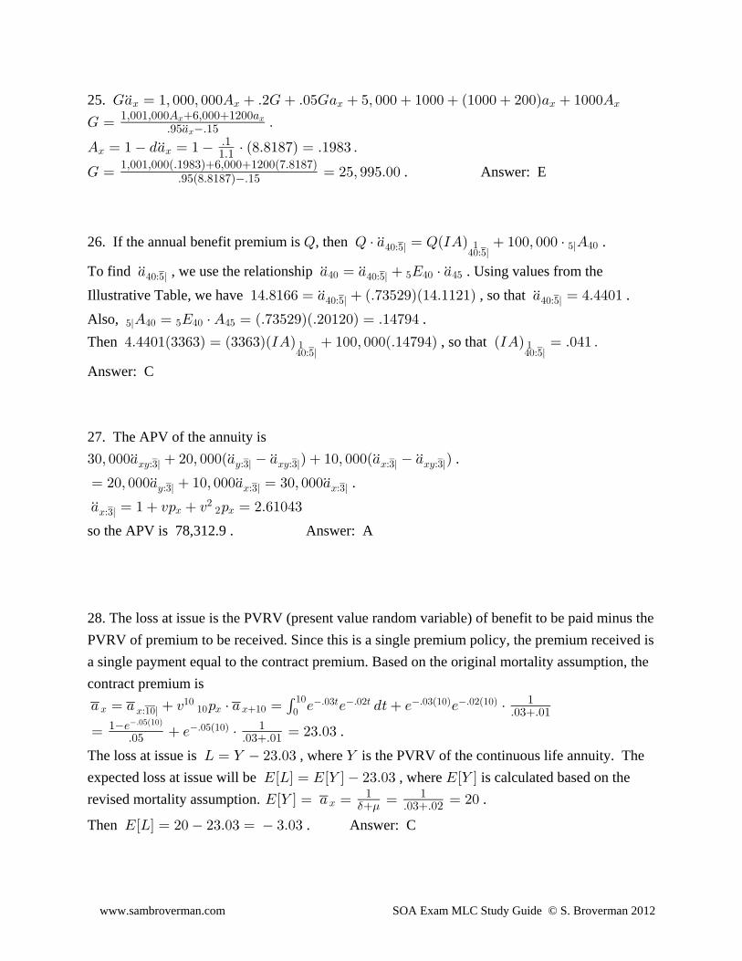
25. K+ œ "ß !!!ß !!!E Þ#K Þ!&K+ &ß !!! "!!! Ð"!!! #!!Ñ+ "!!!EÞÞB B B B B

K œ Þ"ß!!"ß!!!E 'ß!!!"#!!+

Þ*&+ Þ"&ÞÞB B

B

E œ " .+ œ " † Ð)Þ)")(Ñ œ Þ"*)$ ÞÞÞ

B BÞ""Þ"

K œ œ #&ß **&Þ!!"ß!!"ß!!!ÐÞ"*)$Ñ'ß!!!"#!!Ð(Þ)")(Ñ

Þ*&Ð)Þ)")(ÑÞ"& . Answer: E

26. If the annual benefit premium is , then .U U † + œ UÐMEÑ "!!ß !!! † EÞÞ%!À&l

%!À&l" &l %!

To find , we use the relationship . Using values from the+ + œ + I † +ÞÞ ÞÞ ÞÞ ÞÞ%!À&l %!À&l%! & %! %&

Illustrative Table, we have , so that ."%Þ)"'' œ + ÐÞ($&#*ÑÐ"%Þ""#"Ñ + œ %Þ%%!"ÞÞ ÞÞ%!À&l %!À&l

Also, .&l %! & %! %&E œ I † E œ ÐÞ($&#*ÑÐÞ#!"#!Ñ œ Þ"%(*%

Then , so that %Þ%%!"Ð$$'$Ñ œ Ð$$'$ÑÐMEÑ "!!ß !!!ÐÞ"%(*%Ñ ÐMEÑ œ Þ!%" Þ%!À&l %!À&l" "

Answer: C

27. The APV of the annuity is

$!ß !!!+ #!ß !!!Ð+ + Ñ "!ß !!!Ð+ + ÑÞÞ ÞÞ ÞÞ ÞÞ ÞÞBCÀ$l CÀ$l BCÀ$l BÀ$l BCÀ$l .

œ #!ß !!!+ "!ß !!!+ œ $!ß !!!+ÞÞ ÞÞ ÞÞCÀ$l BÀ$l BÀ$l .

+ œ " @: @ : œ #Þ'"!%$ÞÞBÀ$l B # B

#

so the APV is 78,312.9 . Answer: A

28. The loss at issue is the PVRV (present value random variable) of benefit to be paid minus the

PVRV of premium to be received. Since this is a single premium policy, the premium received is

a single payment equal to the contract premium. Based on the original mortality assumption, the

contract premium is

+ œ + @ : † + œ / / .> / / † B "! B B"!BÀ"!l

"! Þ!$> Þ!#> Þ!$Ð"!Ñ Þ!#Ð"!Ñ!"! "

Þ!$Þ!"

œ / † œ #$Þ!$"/ "Þ!& Þ!$Þ!"

Þ!&Ð"!ÑÞ!&Ð"!Ñ .

The loss at issue is , where is the PVRV of the continuous life annuity. TheP œ ] #$Þ!$ ]

expected loss at issue will be , where is calculated based on theIÒPÓ œ IÒ] Ó #$Þ!$ IÒ] Ó

revised mortality assumption. .IÒ] Ó œ + œ œ œ #!B

" " Þ!$Þ!#$ .

Then . Answer: CIÒPÓ œ #! #$Þ!$ œ $Þ!$


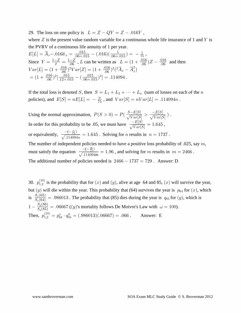
29. The loss on one policy is ,P œ ^ U] œ ^ Þ!"']

where is the present value random variable for a continuous whole life insurance of 1 and is^ ]

the PVRV of a continuous life annuity of 1 per year.

IÒPÓ œ E Þ!"'+ œ ÐÞ!"'ÑÐ Ñ œ

B B"(&

Þ!"& "Þ!'Þ!"& Þ!'Þ!"& ,

Since , can be written as and then] œ œ P P œ Ð" Ñ^ "^ "^ Þ!"' Þ!"'Þ!' Þ!' Þ!'$

Z +<ÒPÓ œ Ð" Ñ Z +<Ò^Ó œ Ð" Ñ Ð E E Ñ Þ!"' Þ!"'

Þ!' Þ!'# # #

B B#

œ Ð" Ñ Ò Ð Ñ Ó œ Þ""%!*%Þ!"' Þ!"& Þ!"&Þ!' Þ"#Þ!"& Þ!'Þ!"&

# # .

If the total loss is denoted , then (sum of losses on each of the W W œ P P âP 8" # 8

policies), and , and .IÒWÓ œ 8IÒPÓ œ Z +<ÒWÓ œ 8Z +<ÒPÓ œ Þ""%!*%88(&

Using the normal approximation, .TÐW !Ñ œ TÐ ÑWIÒWÓ IÒWÓ

Z +<ÒWÓ Z +<ÒWÓ In order for this probability to be .05, we must have ,

IÒWÓ

Z +<ÒWÓ œ "Þ'%&

or equivalently, . Solving for results in . Ñ

Þ""%!*%8

( 8(& œ "Þ'%& 8 8 œ "($(

The number of independent policies needed to have a positive loss probability of .025, say ,7

must satisfy the equation , and solving for results in . Ñ

Þ""%!*%

(

m

m(& œ "Þ*' 7 7 œ #%''

The additional number of policies needed is . Answer: D#%'' "($( œ (#*

30. is the probability that for and , alive at age 64 and 85, will survive the year,: ÐBÑ ÐCÑ ÐBÑ"ß#Ð"!Ñ

but will die within the year. This probability that (64) survives the year is for , whichÐCÑ : ÐBÑ'%

is . The probability that (85) dies during the year is for , which is W Ð'&ÑW Ð'%ÑB

Bœ Þ*)'!"$ ; ÐCÑ)&

" œ Þ!'''( ÐCÑ œ "!! ÞW Ð)'ÑW Ð)&ÑC

C ( 's mortality follows De Moivre's Law with )=

Then, . Answer: E: œ : † ; œ ÐÞ*)'!"$ÑÐÞ!'''(Ñ œ Þ!''"ß# '% )&Ð"!Ñ B C

S. BROVERMAN STUDY GUIDE FOR THE SOCIETY … 3MLC-BRO-12SSM-P... SOA Exam MLC Study Guide © S....

Documents

Transcript of S. BROVERMAN STUDY GUIDE FOR THE SOCIETY … 3MLC-BRO-12SSM-P... SOA Exam MLC Study Guide © S....