RWater, Module 5, November 2015

Created by Adnan Rajib and Venkatesh Merwade, Purdue University 1

Learning Goals

Urbanization refers to the concentration of human populations into discrete areas, leading totransformation of land for residential, commercial and transportation purposes. Such changes in landuseresult into unprecedented changes in ecosystems and environmental processes. From the previousmodules, we have come to know that flow pattern in a stream can be affected by any of the three majorfactors: climatic, geographic as well as human induced changes. Urbanization falls into the ‘humanfactor’ category. After completing this module, students will be able to:

i. see the trend of landuse change in Las Vegas, Nevada, the fastest growing city in the UnitedStates over the past two decades

ii. visualize the possible changes in streamflow for a small watershed in the same area, beingcaused by this ongoing process of urbanization

Visualizing Urbanization Trend in an Area: Example of Las Vegas

The Landsat program is a NASA enterprise for acquisition of satellite imagery of the Earth surface.Following are the true-color Landsat satellite images for Las Vegas, being obtained fromhttp://landsatlook.usgs.gov/, over a period from 1984 to 2014. As these images suggest, Las Vegas hasbeen experiencing rapid urbanization since 1984. In these images, buildings and paved areas appear ingray shades, the clearest example are the sites adjacent to the famous ‘Vegas Strip’ along the centerdiagonal and McCarran International Airport near the bottom center of each image. Grass-covered land,such as parks and golf courses, appears in green.

A video clip showing these ongoing changes can be played from the Google Earth Engine by clicking inthe following link: https://earthengine.google.org/#intro/LasVegas. Run in slow motion for bestvisualization.

19921984

RWater Module 5Hydrograph Analysis to Study the Effect of Urbanization on Streamlow

Adnan Rajib and Venkatesh Merwade

Lyles School of Civil Engineering, Purdue University

RWater, Module 5, November 2015

Created by Adnan Rajib and Venkatesh Merwade, Purdue University 2

Changes in Streamflow with Urbanization

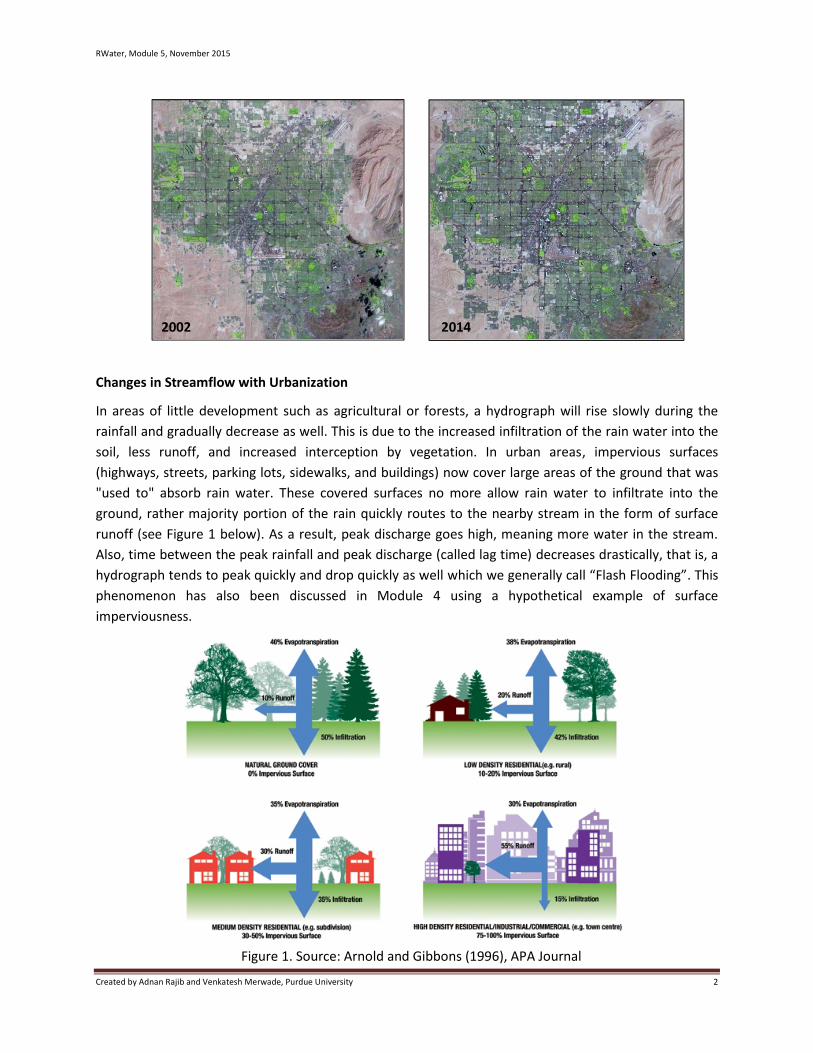
In areas of little development such as agricultural or forests, a hydrograph will rise slowly during therainfall and gradually decrease as well. This is due to the increased infiltration of the rain water into thesoil, less runoff, and increased interception by vegetation. In urban areas, impervious surfaces(highways, streets, parking lots, sidewalks, and buildings) now cover large areas of the ground that was"used to" absorb rain water. These covered surfaces no more allow rain water to infiltrate into theground, rather majority portion of the rain quickly routes to the nearby stream in the form of surfacerunoff (see Figure 1 below). As a result, peak discharge goes high, meaning more water in the stream.Also, time between the peak rainfall and peak discharge (called lag time) decreases drastically, that is, ahydrograph tends to peak quickly and drop quickly as well which we generally call “Flash Flooding”. Thisphenomenon has also been discussed in Module 4 using a hypothetical example of surfaceimperviousness.

2002 2014

Figure 1. Source: Arnold and Gibbons (1996), APA Journal

RWater, Module 5, November 2015

Created by Adnan Rajib and Venkatesh Merwade, Purdue University 3

Now, in order to understand the urbanization effect from a real-time situation we are going todownload the streamflow data at a particular USGS gage station (USGS 09419700) in the Las Vegas cityarea and compare between a past and a more recent time frame (1971-1980 and 2001-2010,respectively). The station we will be studying here as an example is the USGS 09419700, which is theoutlet for the watershed called Las Vegas Wash near Pabco Road. Click on http://goo.gl/Y5lYZZ to seethe watershed as well as the gage station in a customized Google map.

Streamflow data can be downloaded directly by following the script. In addition, two pre-processedrainfall datasets for both time frames are required for this module.

Load the script for this module from your working directory.

Select certain segments of the script and run in steps as shown below.

Make changes only in the portion with "XXXX" or as directed

Relevant explanations associated with each step are also provided here. These explanatory notesare only for building user’s perception over the code.

### STEP 1### Removing previously used scripts from RWater### Removing all previously generated datasets and plotscat("\014")rm(list = ls())dev.off()### STEP 2### Loading a specific package into RWaterlibrary(waterData)### STEP 3### Downloading streamflow data directly from USGS### Save the downloaded data by giving it a name such as 'vegasflow71.80'

vegasflow71.80<-importDVs("XXXX",code="00060", stat="00003",sdate="YYYY-MM-DD",edate="YYYY-MM-DD")

vegasflow01.10<-importDVs("XXXX",code="00060", stat="00003",sdate="YYYY-MM-DD",edate="YYYY-MM-DD")

Provide generic names to the dataframes. It is important to know which columns (more specifically,which data) within your downloaded dataframe you need to use for different analyses. Also, R languageis very case sensitive. You need to be careful in reusing the names of your dataframes to avoid possibleerrors.

A package is a collection of R functions to serve specificanalysis purpose. Package names are case sensitive(waterData: D is capital letter)

In this example, replace XXXX with 09419700.

importDVs is the function name which pulls the data fromUSGS website (case sensitive: D and V are capital letters)

"00060" and "00003" indicates 'Streamflow'and 'Mean Daily Data' respectively

Provide a range of date within sdate andedate in YYYY-MM-DD format. In thisexample, use 2009-01-01 and 2010-12-31respectively

You are saving the downloaded dataframes by givingthem specific names such as vegasflow71.80.

Click on 'vegasflow71.80' or 'vegasflow01.10' (upperright). You will see that streamflow values are listed inthe right column (column header name is val)

RWater, Module 5, November 2015

Created by Adnan Rajib and Venkatesh Merwade, Purdue University 4

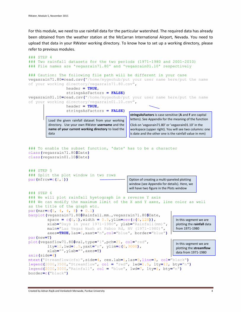
For this module, we need to use rainfall data for the particular watershed. The required data has alreadybeen obtained from the weather station at the McCarran International Airport, Nevada. You need toupload that data in your RWater working directory. To know how to set up a working directory, pleaserefer to previous modules.

### STEP 4### Two rainfall datasets for the two periods (1971-1980 and 2001-2010)### File names are 'vegasrain71.80' and 'vegasrain01.10' respectively

### Caution: The following file path will be different in your casevegasrain71.80=read.csv("/home/mygeohub/put your user name here/put the nameof your working directory/vegasrain71.80.csv",

header = TRUE,stringsAsFactors = FALSE)

vegasrain01.10=read.csv("/home/mygeohub/put your user name here/put the nameof your working directory/vegasrain01.10.csv",

header = TRUE,stringsAsFactors = FALSE)

### To enable the subset function, 'date' has to be a characterclass(vegasrain71.80$Date)class(vegasrain01.10$Date)

### STEP 5### Split the plot window in two rowspar(mfrow=c(2,1))

### STEP 6### We will plot rainfall hyetograph in a reverse Y axis### We can modify the maximum limit of the X and Y axes, line color as wellas the title of the graph etc.par(mar=c(5, 4, 4, 8) + 0.1)barplot(vegasrain71.80$Rainfall.mm.,vegasrain71.80$Date,

space = c(0,1),width = 0.5,ylim=rev(c(0,120)),xlab="Days in year 1971-1980", ylab="Rainfall(mm)",main="Las Vegas Wash at Pabco Rd, NV (1971-1980)",axes=TRUE,las=1,xaxt="n",col="blue", border="blue")

par(new=T)plot(vegasflow71.80$val,type="l",pch=21, col="red",

lty=12,lwd=1.5,yaxt="n", ylim=c(0,3000),xlab="",ylab="",axes=T)

axis(side=4)mtext("Streamflow(cfs)",side=4, cex.lab=1,las=3,line=3, col="black")legend(2000,3500,"Streamflow", col = "red", lwd=1.5, lty=12, bty="n")legend(2000,3000,"Rainfall", col = "blue", lwd=7, lty=1, bty="n")border=c("black")

Load the given rainfall dataset from your workingdirectory. Use your own RWater username and thename of your current working directory to load thedata

stringsAsFactors is case sensitive (A and F are capitalletters). See Appendix for the meaning of the function

Click on 'vegasrain71.80' or 'vegasrain01.10' in theworkspace (upper right). You will see two columns: oneis date and the other one is the rainfall value in mm)

Option of creating a multi-paneled plottingwindow (see Appendix for details). Here, wewill have two figure in the Plots window

In this segment we areplotting the rainfall datafrom 1971-1980

In this segment we areplotting the streamflowdata from 1971-1980

RWater, Module 5, November 2015

Created by Adnan Rajib and Venkatesh Merwade, Purdue University 5

barplot(vegasrain01.10$Rainfall.mm.,vegasrain01.10$Date,space = c(0,1),width = 0.5,ylim=rev(c(0,120)),xlab="Days in year 2001-2010", ylab="Rainfall(mm)",main="Las Vegas Wash at Pabco Rd, NV (2001-2010)",axes=TRUE,las=1,xaxt="n",col="blue", border="blue")

par(new=T)plot(vegasflow01.10$val,type="l",pch=21, col="red",

lty=12,lwd=1.5,yaxt="n", ylim=c(0,3000),xlab="",ylab="",axes=T)

axis(side=4)mtext("Streamflow(cfs)",side=4, cex.lab=1,las=3,line=3, col="black")legend(2000,3500,"Streamflow", col = "red", lwd=1.5, lty=12, bty="n")legend(2000,3000,"Rainfall", col = "blue", lwd=7, lty=1, bty="n")border=c("black")

It is important to understand the expressions or syntax in a programming tool such as RWater.

There can be many columns in one dataframe, each of them holding different sets of values. Bywriting vegasflow01.10$val you are referring to the particular column named as val (thatstores the streamflow values) within the vegasflow01.10 dataframe.

par(new=T) will allow plotting a new graph over the previous graph. In the above example, rainfallbar diagram is plotted first and then streamflow hydrograph is plotted in the same space.

You can get more information about other expressions/commands such as ylim, xlab,lty etc. inthe RWater syntax (see appendix).

The example scripts in this module can be easily reused for any other USGS gage locations, simply bymaking appropriate changes based on your judgment.

Figure 2

RWater, Module 5, November 2015

Created by Adnan Rajib and Venkatesh Merwade, Purdue University 6

Let us now compare the two graphs which we have just created. Read the graphs carefully andcomment on the following statements just by stating TRUE or FALSE:

(i) No drastic changes in the streamflow between the two periods. TRUE/ FALSE(ii) Extreme flows have become more frequent in the recent time period (2001-2010), even under

the same rainfall condition. That means, for the same rainfall magnitude or intensity, thisparticular stream is exhibiting hike in the streamflow values compared to what it used to showin the past. TRUE/ FALSE

These findings can be clarified if we split the whole time frame and re-do the plotting for a very shortperiod of time. In this case, we will compare the streamflow values of February, 1980 and January, 2010.

### STEP 7### Data only for February,1980 and January,2010 is extracted### The new subset datasets are given appropriate nameslibrary(xts)vegasflowFEB1980<-subset(vegasflow71.80,

dates>="1980-02-01"&dates<"1980-03-01")

vegasrainFEB1980<-subset(vegasrain71.80,Date>="1980-02-01"&Date<"1980-03-01")

vegasflowJAN2010<-subset(vegasflow01.10,dates>="2010-01-01"&dates<="2010-01-31")

vegasrainJAN2010<-subset(vegasrain01.10,Date>="2010-01-01"&Date<="2010-01-31")

### STEP 8### Plotting a segment of the whole downloaded time series

# First plot is for February,1980

par(mar=c(5, 4, 4, 8) + 0.1)barplot(vegasrainFEB1980$Rainfall.mm.,vegasrainFEB1980$Date,

space = c(0,1),width = 0.5,ylim=rev(c(0,100)),xlab="Days (Feb, 1980)", ylab="Rainfall(mm)",main="Las Vegas Wash at Pabco Rd, NV (February 1980)",axes=TRUE,las=1,xaxt="n",col="blue", border="blue")

par(new=T)plot(vegasflowFEB1980$val,type="l",pch=21, col="red",

lty=1,lwd=1.5,yaxt="n", ylim=c(0,1000),xlab="",ylab="",axes=T)

axis(side=4)mtext("Streamflow(cfs)",side=4, cex.lab=1,las=3,line=3, col="black")legend(5,1000,"Streamflow", col = "red", lwd=1.5, lty=1, bty="n")legend(5,800,"Rainfall", col = "blue", lwd=7, lty=1, bty="n")border=c("black")

Clipping a date range directly from theoriginal streamflow and rainfall datasets

We need an R package called xts for thesub-setting task

Why is the calling structure of the datecolumn different for rainfall andstreamflow in this example (dates andDate)?

RWater, Module 5, November 2015

Created by Adnan Rajib and Venkatesh Merwade, Purdue University 7

# Second plot is for January,2010barplot(vegasrainJAN2010$Rainfall.mm.,vegasrainJAN2010$Date,

space = c(0,1),width = 0.5,ylim=rev(c(0,100)),xlab="Days (Jan, 2010)", ylab="Rainfall(mm)",main="Las Vegas Wash at Pabco Rd, NV (January 2010)",axes=TRUE,las=1,xaxt="n",col="blue", border="blue")

par(new=T)plot(vegasflowJAN2010$val,type="l",pch=21, col="red",

lty=1,lwd=1.5,yaxt="n", ylim=c(0,3000),xlab="",ylab="",axes=T)

axis(side=4)mtext("Streamflow(cfs)",side=4, cex.lab=1,las=3,line=3, col="black")legend(5,3000,"Streamflow", col = "red", lwd=1.5, lty=1, bty="n")legend(5,2500,"Rainfall", col = "blue", lwd=7, lty=1, bty="n")border=c("black")

The two plots which you have just created show the streamflow hydrograph of the Las Vegas Wash riverin a pre-development and post-development event. Note that, the rainfall pattern in these two separateevents is nearly the same. However, what differences can you see in the respective streamflowresponse?

Figure 3

RWater, Module 5, November 2015

Created by Adnan Rajib and Venkatesh Merwade, Purdue University 8

Quiz

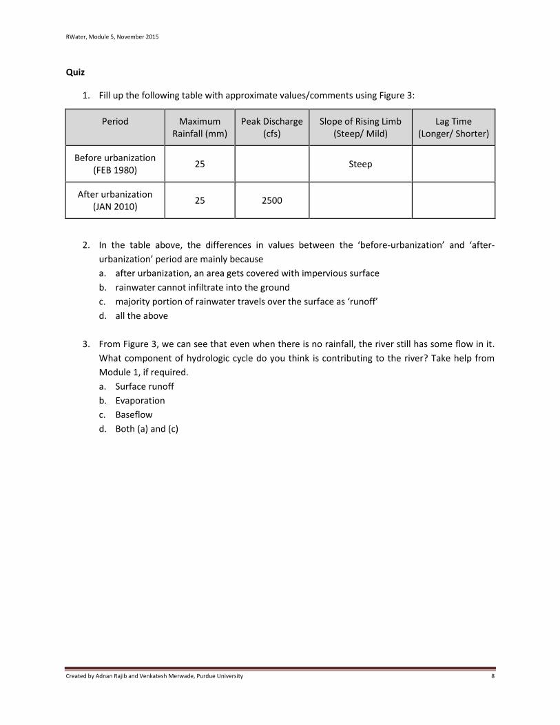
1. Fill up the following table with approximate values/comments using Figure 3:

Period MaximumRainfall (mm)

Peak Discharge(cfs)

Slope of Rising Limb(Steep/ Mild)

Lag Time(Longer/ Shorter)

Before urbanization(FEB 1980)

25 Steep

After urbanization(JAN 2010)

25 2500

2. In the table above, the differences in values between the ‘before-urbanization’ and ‘after-urbanization’ period are mainly becausea. after urbanization, an area gets covered with impervious surfaceb. rainwater cannot infiltrate into the groundc. majority portion of rainwater travels over the surface as ‘runoff’d. all the above

3. From Figure 3, we can see that even when there is no rainfall, the river still has some flow in it.What component of hydrologic cycle do you think is contributing to the river? Take help fromModule 1, if required.a. Surface runoffb. Evaporationc. Baseflowd. Both (a) and (c)