Rwa density what lies behind this underrated financial ratio

Chappuis Halder & Co.

RWA density | What lies behind this underrated

financial ratio

30/01/2016

By Léonard BRIE & Hélène FRÉON

Supported by Benoit GENEST

Global Research & Analytics1

1 This work was supported by the Global Research & Analytics Dept. of Chappuis Halder & Co.

E-mail: [email protected]; [email protected]

© Global Research & Analytics Dept.| 2016 | All rights reserved

2

Table of contents

ABSTRACT 4

INTRODUCTION 5

1. ORIGINS, DEFINITION AND INTRODUCTION TO THE RATIO 6

What are RWA? ........................................................................................................................ 6

An increasingly demanding regulatory context ...................................................................... 7

1.2.1. From Basel II to Basel III 7

1.2.2. Recent evolutions: towards more standardisation and transparency 7

1.2.3. Definition and formula 8

1.2.4. A new monitoring indicator for banks 8

1.2.5. Controversy and questions over the RWA density 9

2. BEYOND THE RWA DENSITY: CHALLENGES AND EVOLUTIONS 10

RWA density sensitivity, applied to theoretical portfolios .................................................. 10

Risk / Profitability cross-analysis: what can we learn from RoRWA? ............................... 15

2.2.1. Presentation of the top 20 European banks sample 15

2.2.2. What is Return on RWA (RoRWA)? 15

2.2.3. Decoding RoRWA: how to interpret the ratio 17

3. A THEORETICAL APPROACH OF RWA DENSITY COMPARED TO INTERNAL

AND EXTERNAL INDICATORS 20

Comparative analyses of RWA density against internal and external indicators ............. 20

3.1.1. RWA density and credit ratings 20

3.1.2. RWA density and cost of risk 21

RWA density or Solvency Ratio, who to trust? .................................................................... 22

RWA density – conclusions..................................................................................................... 23

4. RWA DENSITIES IN PRACTICE: DISTRIBUTION AND KEY LEARNINGS 24

Methodology and bias ............................................................................................................. 24

Preamble................................................................................................................................... 24

4.2.1. RWA for credit risk, key driver of the variations of total RWA 24

4.2.2. Limits in the comparative study of RWA density 26

Key learnings – Analysis of the distribution of historical RWA density ............................ 28

4.3.1. Preliminary analysis: distribution of the sample over the 2012-2014 period 28

4.3.2. Key learnings: distribution of the average RWA density per type of activity 29

Distribution of the sample from various perspectives .......................................................... 30

4.4.1. Distribution of the sample per type of activity 30

4.4.2. Distribution of RWA density average per group and subgroup 31

4.4.3. One step further: what is the contribution of the subgroup analysis? 33


3

Behavioural analysis of the sample ........................................................................................ 34

4.5.1. Methodology and definitions 34

4.5.2. What are the lessons from the behavioural analysis? 35

Trends between the RWA density, total assets and cost of risk .......................................... 36

CONCLUSION 38

TABLE DES ILLUSTRATIONS 39

TABLES 39

BIBLIOGRAPHY 40


4

RWA density | What lies behind this underrated financial ratio

Abstract

The objective of this article is to provide a new angle to the study of RWA density. The worth of this

ratio, created and largely used by financial analysts, has long been underestimated by banks. Yet as

analyses show, this tool may enable a more subtle approach to risk appraisal within a financial

institution.

The first part of this article will cover the origins of the ratio and the history of its use in financial

analysis. The second part will showcase its characteristics and behavioural traits (including during stress

periods), exemplified through a number of theoretical tests. It will be followed by a cross-analysis of

the ratio with other indicators that will help underline the informative and predictive value of RWA

density.

Finally, the last two parts of the article will put the theoretical value of RWA density to the test, by

conducting a practical analysis of its behaviour in Europe over the 2012-2014 period.

The conclusion will appraise the usage and evolution needed to improve and refine the ratio, in order to

monitor scarce resources.

Keywords: financial institutions, risk management, total assets, Basel regulation, Risk-Weighted Assets

(RWA), RWA density, stress testing, internal parameters, profit before tax, Return on RWA (RoRWA)

JEL Classification: C1, G21, G28, G32


5

Introduction

Following the rise of regulatory issues in the monitoring of bank activity, the implementation of Risk-

Weighted Assets for risk management purposes has led to the creation of a new synthetic indicator, the

RWA density. Its goal is to better monitor the risk profile of a balance sheet.

Aside from the classic indicators, financial institutions and markets consider RWA density as the gold

standard for inter- and intra-bank comparisons.

While many critics have cast doubt over the accuracy and relevance of these comparisons, recent

regulatory evolutions (including the new Basel III framework) have had a tendency to reduce the

analytical bias and ease comparisons between the different actors on the market, at least at the European

level.

Taking into account the common efforts made by banks and regulators – especially in Europe – to

provide a uniform and transparent risk assessment environment, it is highly likely that the RWA density

will become an indispensable tool in the coming years for banks to better monitor their internal activities,

or compare themselves to their peers.

The objective of this article is to fully understand the uses of the RWA density. It must also define the

context of its use, so as to better grasp its potential whether it is used as a benchmarking or as a

monitoring tool, or combined with other scarce resources monitoring indicators.

After introducing the ratio through its origins and context, the article will first focus on a theoretical

analysis of the ratio and its behaviour in a controlled space. The conclusions of the first part will then

be pitted against the reality of the European financial sector during the 2012-2014 period.


6

1. Origins, definition and introduction to the ratio

In this section are presented the foundations of the creation of RWA density as a risk management tool

as well as its limitations.

Indeed, from the regulatory environment and the establishment of RWA, is born the need for

standardization and transparency of risk management practices in banks.

What are RWA?

Risk-Weighted Assets, or RWA, represent the amount of risk tied to an asset belonging to a financial

institution. This amount is then converted to the amount of regulatory capital that must be held to reflect

the financial stability of the institution. For every asset, there is a corresponding weight of risk tied to it.

The riskier the asset, the heavier the weight, and the more capital must be held.

The weighting is attached following one of two approaches,

– The “standard approach”: all the weightings are defined by regulation following a fixed-rate

approach

– The “internal approach”: all the weightings are calculated by each bank depending on risk

parameters (CCF/PD/LGD) unique to each asset and defined internally.

Below figure 1 illustrates the classic breakdown of RWAs observed in banks.

Figure 1 RWA description – from a consolidated and detailed perspective

Source: GRA

SubsidiariesCountry

Bank | Consolidated RWA

Split

Operational RWA Market RWA Credit RWA

IRB ApproachStandard Approach

Split

Corporates Banks RetailSovereigns

Mortgage Other retailRevolving


7

An increasingly demanding regulatory context

1.2.1. From Basel II to Basel III

The reinforcement of the banks’ balance sheets has been a priority of the Basel comity ever since the

establishment of its first prudential measures. Its recommendations have been regularly toughened in

order to finally become a set of harmonised obligations for all banks. From Basel I to Basel II and now

Basel III, the evolution has been considerable and increasingly strict.

Following this, banks must now anticipate these measures in order to abide by the new regulatory

prudential obligations in time.

The implementation of the Basel III reforms is part of a set of measures decided upon to reinforce the

financial system following the 2007 financial crisis, and aims to significantly increase the quality of

capital requirements for banks.

This translates mainly into the following measures:

– Increase the level and quality of capital requirements (tier one and core one);

– Implement a leverage ratio;

– Improve liquidity risk management tools by creating two liquidity ratios (1-month liquidity ratio

or LCR, and 1-year liquidity ratio or NFSR);

– Increase the prudential requirements concerning credit counterparty risk (CCR);

– Increase oversight on market activity;

The aim of these measures is to let banks anticipate and absorb shocks caused by future economic crises.

In order to fulfil this objective, it is important to standardise and increase transparency in risk

assessment methods to allow better comparisons between financial institutions. This analysis can

be further refined by asset class or geography, furthermore highlighting the need for consistency

between RWA.

As a matter of fact, it is the goal of Basel III to set itself as the international prudential regulatory standard

in the very near future.

1.2.2. Recent evolutions: towards more standardisation and transparency

In order to converge toward one international, prudential regulatory framework, two types of measures

are needed: an increased transparency and a global standardization of risk control methods.

Standardization of banking risk management practices

The will to harmonise practices and reduce differences in RWA calculation methods (LGD, EAD, PD)

between banks has led to a new regulatory paradigm, wherein banks now share more transparent risk

management practices.

Making banks more transparent

In 2012, following the economic crisis, the European Banking Authority (EBA) introduced a new

recapitalization analysis drill, as part of a series of measures set to restore trust toward European markets.

This consultation brought to light the capitalization weaknesses of a number of banks, and the regulatory

need for more transparency in banking practices.

These efforts were followed in 2013 and, more recently, in November 2015 by the creation by the EBA

of so-called “transparency exercises”, which aggregated large amounts of data to produce comparative

analyses of European banks.

These European “transparency exercises” cover a wide range of indicators that fallow key metrics:

balance sheet management, profitability, liquidity, credit quality and performance. More and more banks

take part in these exercises, allowing European financial markets to use common, standardised indicators

to compare banks across a wide spectrum of metrics.


8

This standardization trend has pushed banks to reassess their RWA calculation methods and production.

Likewise, regulators and financial analysts are now looking at the best standard indicators to accurately

compare banks.

From transparency to standardization: new indicators for comparative analyses

The aim of these evolutions was to ease comparisons between banks for regulatory purposes. This has

been the case with the implementation of the general banking review (AQR, MQR), or the creation of

scoring indicators between banks (SREP). These initiatives pave the way for large-scale analyses taking

into account all regulatory indicators (COREP, FINREP).

1.2.3. Definition and formula

In the last decade, a new indicator has been used by banks and financial analysts alike. It is called the

RWA density ratio, or RWAd, produced by dividing the sum of weighted-risk assets (RWAcredit,

RWAmarket, and RWAoperational) by the sum of the bank’s assets.

𝑅𝑊𝐴𝑑𝑒𝑛𝑠𝑖𝑡𝑦(𝑦) 𝑜𝑢 𝑅𝑊𝐴𝑑(𝑦) =𝑅𝑖𝑠𝑘 𝑊𝑒𝑖𝑔ℎ𝑡𝑒𝑑 𝐴𝑠𝑠𝑒𝑡𝑠𝑡𝑜𝑡𝑎𝑙𝑠 (𝑦)

𝑇𝑜𝑡𝑎𝑙 𝐴𝑠𝑠𝑒𝑡𝑠(𝑦)

Or, for a given year y:

𝑅𝑖𝑠𝑘 𝑊𝑒𝑖𝑔ℎ𝑡𝑒𝑑 𝐴𝑠𝑠𝑒𝑡𝑠𝑡𝑜𝑡𝑎𝑙𝑠 (𝑦) is the sum of RWA credit, market and operational for a given year y:

– 𝑅𝑊𝐴𝑡𝑜𝑡𝑎𝑙𝑠(𝑦) = ∑ 𝑅𝑊𝐴𝑐𝑟e𝑑𝑖𝑡(𝑦) + 𝑅𝑊𝐴𝑚𝑎𝑟𝑘𝑒𝑡(𝑦) + 𝑅𝑊𝐴𝑜𝑝𝑒𝑟𝑎𝑡𝑖𝑜𝑛𝑎𝑙(y)

– 𝑇𝑜𝑡𝑎𝑙 𝐴𝑠𝑠𝑒𝑡𝑠(𝑦) is the sum of assets declared for year y

The result is a synthetic ratio of the amount of risk taken by a bank compared to its assets. This indicator

becomes all the more accurate in the previously explained context of transparency and standardization

of risk calculation methods between banks.

1.2.4. A new monitoring indicator for banks

With a regulatory context that strongly pushes banks to improve their risk measurement methods, be it

in terms of methodology or of parameter calibration (PD and LGD), the latter have focused their efforts

in that direction over the last twenty years.

Unlike the RWA, the RWA density is not a regulatory indicator. Instead, it is the creation of financial

analysts intent on comparing risk profiles between banks. This ratio is all the more useful as it can be

refined to cover a particular sector, region, business activity, etc.

A strategic business dimension

Breaking down RWAs allows for the calculation of RWA density by activity, sector, country or

counterparty, as long as the denominator follows the same breakdown. For example, it is possible to

calculate a sector-specific RWA density as follows:

𝑅𝑊𝐴 𝑑𝑒𝑛𝑠𝑖𝑡𝑦 𝑠𝑒𝑐𝑡𝑜𝑟𝑖𝑎𝑙 (𝑦) =𝑅𝑊𝐴 𝑠𝑒𝑐𝑡𝑜𝑟𝑖𝑎𝑙𝑡𝑜𝑡𝑎𝑙𝑠 (𝑦)

𝑆𝑒𝑐𝑡𝑜𝑟𝑖𝑎𝑙 𝑇𝑜𝑡𝑎𝑙 𝐴𝑠𝑠𝑒𝑡𝑠 (𝑦)

It is thus possible for a bank to contextualise the results of its global RWA density by providing an

adjusted RWA density for each of its business activities, allowing to pilot its risk by activity.

Thanks to its modular structure, banks can thus use the RWA density as a strategic monitoring tool to

analyse key issues or challenges.


9

An evolution in banking monitoring practices

Following increased regulatory pressures on financial markets, banks are now tasked with a complex

exercise: manage their activity following the key objectives of liquidity, profitability, and refinancing,

all the while managing regulatory expectations in terms of solvency, balance sheet, and risk

management.

To that end, the RWA density appears as a key ratio. Heavily criticised yet broadly used by investors

and banks alike, the ratio displays its value when used in conjunction with other indicators, both external

(i.e. credit ratings) and internal (i.e. profitability and solvency ratios).

The cross-analyses featured in part 3 tend to confirm this assumption, which suggests a brighter future

for RWA density as a key bank-monitoring indicator.

1.2.5. Controversy and questions over the RWA density

Investors were quick to pick up the RWA density as a useful synthetic indicator to direct their

investments, a position soon picked by banks.

However, in the last years some voices have been heard questioning both the quality of the ratio and the

relevance of the analyses derived from it.

Nevertheless, the aim of this article is not to question the construction of the ratio or its relevance, but

instead to focus on its strengths, all the while mitigating its limits.


10

2. Beyond the RWA density: challenges and evolutions

While the previous section aimed at explaining the breakdown of the RWA density, it did not detail its

theoretical or behavioural components. The aim of this part is thus to understand the underlying

theoretical components of the ratio and understand how it behaves, particularly during stress periods.

RWA density sensitivity, applied to theoretical portfolios

While the synthetic nature of the RWA density makes it a useful comparison tool, the low number of

indicators it encompasses can also be a weakness. Indeed, the RWA credit typically accounts for 80%

of the RWA density (as illustrated in 4.2.1). This ratio relies on internal parameters like Probability of

Default (PD), Loss Given Default (LGD) and Exposure At Default (EAD). Taking these parameters into

account in the calculation of the RWA density, one could think that risks taken by financial

establishments can easily be compared.

However, it is possible that banks take risks of differing nature yet that their RWA density converge

towards a similar level. The aim of this section is thus to test the sensitivity of the RWA density towards

their internal risk parameters.

Taking into account the fact that the RWA density essentially rest upon credit risks, our study focuses

on credit portfolios of two fictional banks with retail exposure, but could be widened to take into account

corporate, financial institutions or sovereigns exposures.

Description of the bank I

The breakdown of the portfolio of bank I is shown below.

Table 1 Portfolio composition of the bank I

Source: GRA

This first bank is engaged in a diversified retail activity, with exposure similarly allocated within all

services (mortgage, revolving, other retail – secured or unsecured), and it favours its good clients. For

each activity, population is mainly split among the least risky classes (risk class from 1 to 5).

The RWA of this portfolio (20 783€) divided by the total assets of the bank (173 188€) amounts to

a level of RWA density of 12%.

Total RWA 20 783

Total Assets 173 188

RWA density 12,00%

Mortgage

Class Populations EAD PD LGD rw RWA RWA d

1 18% 3 600 0,15% 10,00% 3,43% 123 0,1%

2 23% 4 600 0,20% 10,00% 4,25% 196 0,1%

3 16% 3 200 0,40% 10,00% 7,05% 226 0,1%

4 16% 3 200 0,75% 10,00% 10,94% 350 0,2%

5 15% 3 000 0,90% 10,00% 12,38% 371 0,2%

6 6% 1 200 1,50% 10,00% 17,30% 208 0,1%

7 6% 1 200 2,20% 10,00% 21,95% 263 0,2%

Total 20 000 8,69% 1 738 1,0%

Other retail - secured


1 17% 3 400 0,15% 10,00% 3,52% 120 0,07%

2 21% 4 200 0,20% 10,00% 4,29% 180 0,10%

3 21% 4 200 0,40% 10,00% 6,70% 281 0,16%

4 18% 3 600 0,75% 10,00% 9,45% 340 0,20%

5 14% 2 800 0,90% 10,00% 10,29% 288 0,17%

6 5% 1 000 1,50% 10,00% 12,57% 126 0,07%

7 4% 800 2,20% 10,00% 13,97% 112 0,06%

Total 20 000 7,23% 1 447 0,8%

Other retail - unsecured


1 18% 3 600 0,15% 30,00% 10,56% 380 0,2%

2 23% 4 600 0,50% 30,00% 22,87% 1 052 0,6%

3 16% 3 200 0,75% 30,00% 28,34% 907 0,5%

4 12% 2 400 0,90% 30,00% 30,88% 741 0,4%

5 19% 3 814 2,00% 30,00% 40,98% 1 563 0,9%

6 6% 1 200 5,00% 30,00% 46,93% 563 0,3%

7 6% 1 200 7,50% 30,00% 49,56% 595 0,3%

Total 20 000 29,00% 5 801 3,3%

Revolving


1 35% 7 000 0,90% 75,00% 28,07% 1 965 1,1%

2 25% 5 000 1,80% 75,00% 47,30% 2 365 1,4%

3 20% 4 000 3,30% 75,00% 73,01% 2 920 1,7%

4 15% 3 000 5,00% 75,00% 96,72% 2 901 1,7%

5 2% 425 7,30% 75,00% 123,06% 523 0,3%

6 2% 384 9,00% 75,00% 139,50% 535 0,3%

7 1% 282 20,00% 75,00% 208,44% 587 0,3%

Total 20 000 58,99% 11 798 6,8%


11

Figure 2 Distribution of RW and RWA densities – Bank I

Source: GRA

Description of bank II

The breakdown of the portfolio of bank II is shown below.

Table 2 Portfolio composition of the bank II

Source: GRA

Unlike the first bank, this establishment focuses its retail activity on secured products (mortgage and

other retail – secured) and tries to minimise its loss rates regardless of the risk class of its customers.

The RWA of this portfolio (12 820€) divided by the total assets of the bank (106 835€) amounts to

a level of RWA density of 12%.

Mortgage8,7%


7,2%


29,0%

Revolving59,0%

Risk Weighted

Mortgage1,0%


0,8%


3,3%

Revolving6,8%

RWA density

Total RWA 12 820

Total Assets 106 835

RWA density 12,00%

Mortgage


1 10% 4 000 0,10% 10,00% 2,52% 101 0,1%

2 18% 7 200 0,15% 10,00% 3,43% 247 0,2%

3 12% 4 800 0,40% 10,00% 7,05% 339 0,3%

4 10% 4 000 0,90% 10,00% 12,38% 495 0,5%

5 20% 8 000 1,50% 10,00% 17,30% 1 384 1,3%

6 20% 8 000 2,00% 10,00% 20,71% 1 657 1,6%

7 10% 4 000 5,00% 10,00% 34,91% 1 397 1,3%

Total 40 000 14,05% 5 619 5,3%



1 9% 2 700 0,10% 10,00% 2,63% 71 0,1%

2 15% 4 500 0,15% 10,00% 3,52% 158 0,1%

3 15% 4 500 0,40% 10,00% 6,70% 301 0,3%

4 11% 3 300 0,90% 10,00% 10,29% 340 0,3%

5 25% 7 500 1,50% 10,00% 12,57% 943 0,9%

6 13% 3 900 2,00% 10,00% 13,66% 533 0,5%

7 12% 3 600 5,00% 10,00% 15,64% 563 0,5%

Total 30 000 9,70% 2 909 2,7%



1 13% 650 0,15% 20,00% 7,04% 46 0,0%

2 23% 1 150 0,50% 20,00% 15,25% 175 0,2%

3 18% 900 1,00% 20,00% 21,56% 194 0,2%

4 10% 500 1,50% 20,00% 25,14% 126 0,1%

5 16% 800 3,00% 20,00% 29,58% 237 0,2%

6 10% 500 5,50% 20,00% 31,59% 158 0,1%

7 10% 500 8,00% 20,00% 33,49% 167 0,2%

Total 5 000 22,06% 1 103 1,0%

Revolving


1 20% 1 000 0,75% 60,00% 19,50% 195 0,2%

2 22% 1 100 2,00% 60,00% 40,88% 450 0,4%

3 20% 1 000 3,50% 60,00% 60,83% 608 0,6%

4 14% 700 5,00% 60,00% 77,37% 542 0,5%

5 13% 650 7,00% 60,00% 95,93% 624 0,6%

6 8% 400 11,00% 60,00% 125,05% 500 0,5%

7 3% 150 25,00% 60,00% 180,49% 271 0,3%

Total 5 000 63,78% 3 189 3,0%


12

Figure 3 Distribution of RW and RWA densities – Bank II

Source: GRA

Description of the stress scenarios

The portfolios of both banks are clearly different. Hence they are not subject to the same risks

although their RWA density are identical.

In order to observe the sensitivity of the RWA density with regards to internal parameters – and thus the

risks facing each bank –, various stress scenarios are applied and allocated on a fixed-rate basis.

Each scenario is based on the deterioration of the PD, LGD, or credit migration, allowing the

measurement of the level of the RWA density under stress conditions.

The basis of each scenario is presented below.

The first scenario recreates the effects of a real estate crisis for each bank. The revolving portfolio is

not affected, as it is not sensitive to the real estate market.

In the other portfolios, credit migration towards risker credit classes can be observed. In portfolios where

the recovery rates depend on the value of the property (mortgage and other retail – unsecured) an

aggravation of LGD is applied; for other retail – unsecured portfolio the LGD remain steady since the

guarantor is obliged to pay.

The second scenario describes an economic crisis (rise of the unemployment rate and impact on the

inflation) where only revolving and other retail – unsecured are impacted. So for the concerned

portfolios, the effects are a migration of populations in the riskiest classes, an aggravation of the PD and

LGD.

The third scenario corresponds to a recovery rates stress, resulting in a worsening of LGD on all the

portfolios.

Mortgage14,0%


9,7%


22,1%

Revolving63,8%

Risk Weighted

Mortgage5,3%


2,7%


1,0%

Revolving3,0%

RWA density

Real estate crisis – Impact on mortgage and other retail portfolio• Migration of populations in the riskiest classes • LGD Aggravation – mortgage and other retail unsecured• LGD stable – other retail secured

Scenario 1

Migration - pop -2% -2% -1% 1% 1% 2% 1%

LGD 20%

Economic crisis – Impact on revolving and other retail portfolio• Migration of populations in the riskiest classes • PD Aggravation• LGD Aggravation

Scenario 2

LGD 10%

Migration - pop -5% -5% -2% 2% 3% 5% 2%

PD Aggravation 0,3% 0,3% 0,3% 0,5% 0,4% 0,0% 0,0%

Stress on recovery - Impact on all the portfolios• LGD Aggravation

Scenario 3

LGD 10%


13

The fourth scenario corresponds to default rates stress, resulting in an intensification of PD on the least

risky classes and specific to each portfolio.

The fifth scenario is the combination of the third and fourth scenario.

The last scenario represents a global stress impacting all portfolios and resulting in a migration of

populations in the riskiest classes, an aggravation of LGD and PD on the least risky categories specific

to each portfolio.

Analysis of the results of all stress scenarios

Levels of RWA densities and variations observed for each scenario are the following.

Table 3 RWA densities for each scenario

Source: GRA

In the case of the least penalising scenarios (1 to 4), RWA density levels for bank I show little variation,

which is not the case for bank II, where these levels are heavily impacted for scenarios 1 and 3.

This has to do with portfolio structure of both banks. Highly diversified bank I is less sensitive to one

parameter suddenly worsening, whereas LGD aggravation on its secured portfolios lead bank II to

double its levels of RWA density.

Still concerning bank II, scenarios impacting non-secured activities or worsening default probabilities

only have a minimal effect on RWA density.

When comparing RWA density levels between banks I and II for serious, global scenarios, it is shown

that bank I is less at risk than bank II.

So while these banks initially show similar levels of risk, these stress exercises show that initial

observation is not always correct.

The synthetic nature of RWA density makes it blind to certain risk exposures or investment

strategies taken by banks.

In addition to the various stress scenarios, a PD stress simulation method for each risk class was

implemented in order to verify RWA density sensitivity to stress.

PD stress for each portfolio is defined as follows. For each risk class, the 95% quantile of PD is derived

using Vasicek’s formula:

Stress on default rates - Impact on all the portfolios• PD Aggravation on all the least risky classes

Scenario 4

PD Aggravation - Mortgage 0,3% 0,3% 0,3% 0,0% 0,0% 0,0% 0,0%

PD Aggravation - Unsecured 0,3% 0,2% 0,1% 0,0% 0,0% 0,0% 0,0%

PD Aggravation - Revolving 1,0% 1,0% 1,0% 0,0% 0,0% 0,0% 0,0%

Stress on default rates and recovery - Impact on all the portfolios• PD Aggravation on all the least risky classes • LGD Aggravation

Scenario 5

LGD 10%




Global stress - Impact on all the portfolios• Migration of populations in the riskiest classes• PD Aggravation on all the least risky classes • LGD Aggravation

Scenario 6

LGD 10%

Migration pop -5% -5% -2% 2% 3% 5% 2%




RWA d - Initial RWA d Variation RWA d Variation RWA d Variation RWA d Variation RWA d Variation RWA d Variation

Bank 1 12% 17% 39% 17% 45% 16% 32% 15% 21% 19% 60% 21% 76%

Bank 2 12% 25% 106% 14% 17% 21% 75% 13% 12% 24% 96% 26% 114%

Scenario 6Scenario 1 Scenario 2 Scenario 3 Scenario 4 Scenario 5


14

q(PD; x%) = 𝒩 (𝒩−1(PD) + √R ∗ 𝒩−1(x%)

√1 − R)

– Where R is the correlation coefficient, fixed at 4% and 15% for revolving and mortgage

portfolio respectively; and is calculated following the Basel formula for other retail portfolio:

R = 0.03 (1 − e−35∗PD

1 − e−35 ) + 0.16 (1 −1 − e−35∗PD

1 − e−35 )

– Then the stressed PD for risk class 1 is simulated as a random draw of a uniform law, PDs(1) ~

U (PD(1), q(PD(1), 95%)).

– For all the others risk classes i ϵ {2, 3, 4, 5, 6,7}, the stressed PD is simulated as a random draw

of a uniform law, PDs(i) ~ U (max (PD(i), PDs(i-1)), q(PD(i), 95%)).

The results after a thousand simulations of RWA density for both banks are presented in the figure

below.

Figure 4 Compared distribution of stressed RWA densities by banks

Source: GRA

Table 4 Statistics of stressed RWA densities by bank

Source: GRA

As shown previously by scenario 4 of the study, the first bank is more sensitive to stress of default

probability than the second bank, which is reflected in its RWA density values.

Knowing the relationship between RWA density and others financial indicators, such as external rating

(cf. 3.1.1), variations of RWA density could help a bank anticipate the impact of a stress on its rating.

Likewise with the implementation of SREP, a rating set by the central bank in order to grade banks

following a regulatory method, any link between this score and the RWA density would also allow banks

to manage and anticipate change in their rating.

To conclude, these studies show that analyses of the changes of RWA density under miscellaneous

stress scenarios strengthen the comparison of bank solidity, and may allow this indicator to better

manage business activities or stress. Contrary to RWA, changes of RWA density help highlight

0,6%

2,8%

8,9%

20,9%

19,5%

20,6%

16,4%

7,3%

2,2%

0,6%

0,2%

[29%; 29,5%]

[29,5%; 30%]

[30%; 30,5%]

[30,5%; 31%]

[31%; 31,5%]

[31,5%; 32%]

[32%; 32,5%]

[32,5%; 33%]

[33%; 33,5%]

[33,5%; 34%]

[34%; 34,5%]

Bank 1| Repartition of stressed RWA densities

0,1%

1,2%

4,9%

14,3%

23,7%

25,7%

20,4%

8,5%

1,1%

0,1%

[20,5%; 21%]

[21%; 21,5%]

[21,5%; 22%]

[22%; 22,5%]

[22,5%; 23%]

[23%; 23,5%]

[23,5%; 24%]

[24%; 24,5%]

[24,5%; 25%]

[25%; 25,5%]

Bank 2 | Repartition of stressed RWA densities

mean standard deviation Empirical CI - 95%

Bank n°1 31,4% 0,8% [29,9%; 33,1%]

Bank n°2 23,1% 0,7% [21,7%; 24,4%]

RWA density


15

institutions showing risks that appear similar but are actually of differing natures, as well as reveal

previously hidden or unanticipated risks.

Risk / Profitability cross-analysis: what can we learn from RoRWA?

Profitability and Risk Management indicators are interesting to cross-analyse since they illustrate the

typical trade-offs a bank must face on a daily basis – that is taking risks in order to get returns.

The following part will therefore provide an analysis based on two sets of historical data.

(1) Set 1 comprises 13 top European banks where key Risk Management and Profitability indicators

have been collected for the 2006-2011 period, such as: Total Assets (TA), Net Banking Income

(NBI), Cost of Risk (CoR), Consolidated Net Income. Those banks are included in Set 2.

(2) Set 2 (top-20 European banks sample) includes 20 European banks, described in the following

paragraph (cf. 2.2.1). This set will be reused for the purpose of analyses on part 3 and 4. Data

collection comprises data collected for Set 1 (cf. above), and the following indicators: Total

Risk-Weighted Assets (RWA), Before-Tax Income (BTI) and Return on RWA (RoRWA).

2.2.1. Presentation of the top 20 European banks sample

This article will capitalise on the analysis provided on the following 20-top European banks (in asset

volumes as of 31/12/2012). Data has been collected for each banking exercise (2012, 2013, and 2014)

from the publicly published annual reports and income statements. Analyses will be provided on

consolidated data at group level, cross-activities / cross-entities for every bank of the sample.

The 20-top EU banks of Set 2 respectively represent 72% (as for the 2012 exercise) and 68% (as for the

2014 exercise) of total Risk-Weighted Assets of the Euro-Zone2.

Below is the list of the banks comprised in the sample and their respective reference, depending on their

home country:

– 2 Swiss banks (CH1; CH2)

– 2 German banks (DE1; DE2)

– 2 Spanish banks (ES1; ES2)

– 5 French banks (FR1; FR2; FR3; FR4; FR5)

– 2 Italian banks (IT1; IT2)

– 2 Dutch banks (NL1; NL2)

– 1 Swedish bank (SW1)

– 4 British banks (UK1; UK2; UK3; UK4)

2.2.2. What is Return on RWA (RoRWA)?

How to calculate Return on RWA?

Below is the formula for Return on RWA (RoRWA):

𝑅𝑜𝑅𝑊𝐴(𝑎) = 𝐵𝑇𝐼 (𝑦)

𝑅𝑊𝐴𝑡𝑜𝑡𝑎𝑙(𝑦)

Where with respect to a given bank, for a given year y:

– BTI (y) = Before Tax Income (y) = NBI (y) – Operational expenses (y) + CoR (y) – Other income and charges (y)

– CoR (y) is defined as the sum of capital charges and loan loss provisions estimated by a bank for a given year y

– 𝑅𝑊𝐴𝑡𝑜𝑡𝑎𝑙(𝑦) = ∑ 𝑅𝑊𝐴𝑐𝑟𝑒𝑑𝑖𝑡(𝑦) + 𝑅𝑊𝐴𝑚𝑎𝑟𝑘𝑒𝑡(𝑦) + 𝑅𝑊𝐴𝑜𝑝𝑒𝑟𝑎𝑡𝑖𝑜𝑛𝑎𝑙(𝑦)

2 Data from the EBA transparency exercise (published in 2013 and 2015), respectively including 17 and 18 of the

20 banks of the sample


16

This ratio links the BTI and the total RWA of a given bank, illustrating its capacity to create value

according to the risks undertaken and translated in RWA.

Before-Tax Income prevails on Net Income since it doesn’t take into account taxes, considered earlier

in this article, as a dependency factor which varies according to the banks’ home country, therefore

biasing the analysis.

Why use RoRWA?

As suggested in Striking the right balance between risk and return (Bain & Company, 2013), this

indicator encompasses two key dimensions at the heart of the traditional Risk / Return banking trade-

off.

Beyond its bi-dimensional character, the analysis of Return on RWA is interesting since Cost of Risk

is an indirect part of the ratio. As a matter of fact, CoR is a cost item of banks’ BIT. The graph below

illustrates in particular the allocation of costs and revenues charged to the NBI for the sample between

2012 and 2014.

The proportion of the cost of risk to NBI has doubled on average over the past 8 years (cf. graph below)

and even increased to 80% for some of the banks in 2008, at a time of crisis. This is key to further the

analysis of RoRWA.

Figure 5 Evolution of the cumulated cost items of the NBI among the 20 banks ( set 2) of

the sample on the 2012-2014 period

Source: GRA

According to CoR and RWA natural correlation (cf. 3.1.2), it is interesting to consider the part of Cost

of Risk in relation to banks’ NBI. The more significant the proportion, the closer Before-Tax Income

and RWA will get indirectly. This tends to be demonstrated in the following paragraphs.

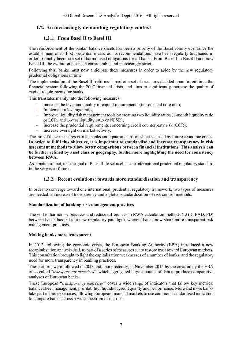
The analysis of historical data of set 1 – 13 top European banks between 2006 and 2011 – demonstrates

that the CoR / NBI ratio has globally increased by an average of 63%, from 6% to 10% while CoR

increased (in value) by an average of 52% on the period (2006-2014).

Furthermore, as illustrated in the figure below, Cost of Risk is very sensitive to stress periods. As a

matter of fact, in 2009, in the wake of the global financial crisis, CoR doubled over the year, while NBI

only dropped by an average of 22.6%.

1 403

383

175 188

1 020

209 13

Net Banking Income Operational charges Cost of Risk Before-Tax Income

15% BTI1% BTI

Net Operating Income

Other income and charges

Gross Operating Income


17

Figure 6 Evolution of the annual mean values of NBI and CoR / NBI between 2006 and

2014 on 13 European banks (set 1)

Source: GRA

What is at stake for EU banks in the context of a growing proportion of CoR to NBI?

For a given European bank, following the 2006-2014 period

– The Net Income might drop, causing an eroded profitability over the years, especially if the NBI

is steady over the years (e.g. above graph on period 2012-2014);

– Profitability (NBI) could be more dependent on Risk Management policy, since correlation

between NBI and RWA will strengthen;

– Profitability will probably be more stress-sensitive due to the growing part of CoR in NBI cost

items.

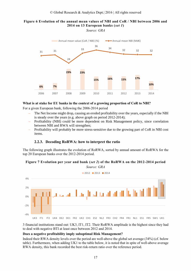
2.2.3. Decoding RoRWA: how to interpret the ratio

The following graph illustrates the evolution of RoRWA, sorted by annual amount of RoRWA for the

top 20 European banks over the 2012-2014 period.

Figure 7 Evolution per year and bank (set 2) of the RoRWA on the 2012-2014 period

Source: GRA

3 financial institutions stand out: UK3, IT1, IT2. Their RoRWA amplitude is the highest since they had

to deal with negative BTI at least once between 2012 and 2014.

Does a negative profitability imply suboptimal Risk Management?

Indeed their RWA density levels over the period are well-above the global set average (34%) (cf. below

table). Furthermore, when adding UK1 to the table below, it is noted that in spite of well-above average

RWA density, this bank recorded the best risk-return ratio over the reference period.

6% 7%

23% 23%

15% 16% 15% 17%

10%

31 31

24

3336

3432 32 32

0

5

10

15

20

25

30

35

40

0%

5%

10%

15%

20%

25%

30%

35%

40%

45%

50%

2006 2007 2008 2009 2010 2011 2012 2013 2014

Annual mean value (CoR / NBI) (%) Annual mean NBI (Md€)

-4%

-2%

0%

2%

4%

UK3 IT1 IT2 UK4 DE2 DE1 FR2 UK2 CH1 ES2 NL2 FR3 CH2 FR4 FR1 NL1 ES1 FR5 SW1 UK1

2012 2013 2014


18

Table 5 Average RWA indicators, compared over the 2012-2014 period for 4 EU banks

Source: GRA

Why are the banks’ average RoRWA so different at comparable RWA density levels?

First of all, the analysis of these 4 banks RWA density and RoRWA challenges some common beliefs

about how banks deal with risk-return trade-offs. As demonstrated in the stress tests analysis (cf. 2.1),

it may not be the amount (quantity) of risks a bank is setting in its balance sheet but the type and solidity

of portfolios (quality) that matters.

This is consistent with UK3 indicators: this financial institution was the least risk-efficient in spite of an

average RWA density compared to the global sample over the period; meaning some institutions with

higher average RWA density performed better on the same time slot.

To take the analysis one step further, the following analyses will focus on a Risk Management indicator

revealing the quality of the risked assets held by the bank – the Cost of Risk over PNB. On the one hand

CoR is a qualitative ratio of risk held by financial institutions; on the other hand the share of CoR in a

bank’s NBI (stable over the period) provides a relevant indicator of banking revenues erosion.

One must nevertheless note that the variations of the CoR / NBI ratio are driven by CoR evolutions over

the period (cf. table below).

Table 6 Variation averages of NBI and CoR compared over 2012-2014 for 4 EU banks

Source: GRA

Figure 8 Annual evolution of the CoR / NBI ratio per EU bank over 2012-2014

Source: GRA

CoR / NBI analysis for the global sample and over the 2012-2014 period provides some key learnings,

especially on the set of 4 banks identified above – UK1, UK3, IT1, IT2.

For a comparable level of RWA density,

– Banks, RoRWA of which is negative (UK3, IT1, IT2), combine above-average RWA density

with large CoR to NBI contribution (higher than 30%), therefore greatly exceeding the period

average (16%).

Banks Mean (RWA d) Mean (RoRWA)

UK3 35% -0,96%

IT1 48% -0,83%

IT2 47% 0,12%

UK1 43% 3,05%

Banks Mean Var(NBI) Mean Var(CoR)

UK3 7,47% -128,17%

IT1 -6,65% -54,62%

IT2 -6,28% -4,58%

UK1 -1,54% -49,51%

0,00%

5,00%

10,00%

15,00%

20,00%

25,00%

30,00%

35,00%

40,00%

45,00%

CH1 CH2 DE1 SW1 UK1 UK4 FR5 FR4 FR1 FR2 NL1 UK2 FR3 DE2 NL2 ES1 ES2 UK3 IT2 IT1

2012 2013 2014


19

– By contrast, UK1, for which the RoRWA was the best between 2012 and 2014, recorded the

least volatile and important amount of CoR / NBI over the period compared to the 3 other banks.

This suggests that for a comparable level of RWA density, Non-Performing Loans (NPL) are actually

eroding banking profitability. Suboptimal lending policies could be a hypothesis for higher volatility in

CoR evolution for a given bank.

What are the key takeaways of RoRWA analysis?

First of all, RWA density is not enough to draw fair conclusions regarding the stability or solvency of a

given bank.

As a matter of fact, for comparable RWA density levels, analyses of other indicators are more relevant

– for example stability of the Cost of Risk and evolution of the share of CoR in NBI. It could be

interesting to fine-tune this risk-return analysis with clusters defined per RWA density range, type of

banking activity, home country etc.

RoRWA analysis highlighted the following key learnings:

(1) On the one hand, maintaining an average level of RWA density, ranging from 30% to 40%, does

not imply a bank will be able to be risk-efficient and create value.

(2) On the other hand, a bank with an above-average RWA density can be profitable if they master

the volatility tied to their cost of risk.

(3) As suggested in 2.1, RWA density analysis does not reveal the qualitative evolution of a bank’s

assets; yet this might erode banking profitability, given the significant part of CoR in the

calculation of the financial results of a bank.

(4) At last, cost of risk is a key indicator, since it represents a growing part of the NBI’s cost items,

particularly sensitive under stress situation.


20

3. A theoretical approach of RWA density compared to internal and

external indicators

Compared with other indicators, RWA density can reveal information previously unseen through stand-

alone analysis. The objective of this section is to highlight existing correlations between RWA density

and other risk management and solvency ratios. This will further help to conclude about the importance

and relevance of the ratio.

Do these indicators provide the same explanatory power? Are they correlated or complementary?

Finally, what are the key understandings and advantages to be drawn from RWA density?

Comparative analyses of RWA density against internal and external

indicators

In the following paragraph, two different key Risk Management measures will be compared to RWA

density for a given sample of financial institutions:

– The first indicator is credit ratings (external indicator), reflecting the credit worthiness of an

investment, representing therefore in the eyes of the investors a good proxy of a bank’s financial

soundness;

– The second indicator is the Cost of Risk / Total Assets ratio (internal indicator) that is the

expected cost of risks for a bank regarding its investments and internal data.

3.1.1. RWA density and credit ratings

The following study uses the data of the banks described in 2.2.1 between 2012 and 2014. Banks are

clustered by ratings (S&P ratings). For each rating, the average RWA density, the minimum and the

maximum are calculated and presented in below Figure 9. This helps to identify the degree of correlation

between RWA density and credit rating per grade.

Figure 9 Distribution of RWA density by external rating between 2012 and 2014

Source: GRA

The above figure highlights the correlation between RWA density and credit rating, yet the link is not

obvious for each rating. Nevertheless, the average RWA density of banks for which the ratings are

ranging from AA- to A- does not exceed 40%; on the contrary the average RWA density of banks for

which ratings are inferior to BBB+ is well-above 40%.

30%32%

28%

32%

51%49% 48%

25%

16%19%

24%

46%44% 43%

33%

46%

37%39%

56% 56%53%

AA- A+ A A- BBB+ BBB BBB-


21

RWA density can thus provide information about the credit worthiness of banks – at least to some extent.

As an example, analysis of average RWAd in this sample clearly provides a vector of differentiation

between Upper medium grade and Lower medium grade institutions.

This is enhanced by measuring the Cramer’s V. The results are presented below in the contingency table

resulting from the sample.

Table 7 Contingency table between credit grade and RWA density over 2012 to 2014

Source: GRA

The degree of association between average RWAd clusters ( 40%; > 40%) and credit ratings is

estimated to 90.2% (Cramer’s V).

This reveals a strong connection between credit ratings – an external indicator – and RWA density

– an internal indicator. Thus it is interesting to verify if those observations are applicable when RWA

density is compared to an internal indicator.

3.1.2. RWA density and cost of risk

Cost of Risk represents the provisions held by a bank to cover payment risks, that is, credit losses and

defaulted amounts. This is calculated as the difference between the total adjustments on impaired assets

included in the income statement and the overall outstanding loans to customers.

As a matter of fact this is an internal and direct assessment of a bank’s own risks. CoR fluctuations are

particularly sensitive to the quality of credit granting processes (internal factor) or to the economic

environment (external factor).

The objective of this paragraph is to compare Cost of Risk and RWA density in order to estimate the

ability of RWAd to assess internal risks for a given bank. For the sake of consistency, RWA density will

be compared to cost of risk over total assets. The results are presented below in Figure 10.

Here, only 19 banks are represented in the correlation study in 2014. 2012 and 2013 analysis concerned

the full sample (20 banks).

Figure 10 Correlations between RWA density and Cost of risk / TA per year

Source: GRA

RWA density <= 40% RWA density > 40%

AA- 5 0

A+ 7 3

A 25 0

A- 8 0

BBB+ 0 3

BBB 0 6

BBB- 0 3

Upper

medium

grade

Lower

medium

grade

y = 25,792x + 0,2263R² = 0,7752

0%

10%

20%

30%

40%

50%

60%

0,0% 0,2% 0,4% 0,6% 0,8% 1,0% 1,2% 1,4%

RW

A d

Cost of Risk / TA

RWAd vs Cost of Risk / TA - 2012

y = 18,185x + 0,2653R² = 0,6617

0%

10%

20%

30%

40%

50%

60%

0,0% 0,5% 1,0% 1,5% 2,0%

RW

A d

Cost of Risk / TA


y = 27,007x + 0,2738R² = 0,5441

0%

10%

20%

30%

40%

50%

60%

0,0% 0,2% 0,4% 0,6% 0,8% 1,0%

RW

A d

Cost of Risk / TA



22

The above figure shows RWA density is highly correlated to the CoR / TA ratio for each year over the

period, correlation coefficients exceeding 74%. As a consequence there is a strong link between those

ratios. This is consistent with the definition of RWAd as an internal risk measurement tool. This is

especially logical since the numerator (RWA) is generally calculated using internal risks parameters

(PD/LGD/CCF).

However the correlation degree is decreasing over the period. This suggests that new indicators are taken

into account in the CoR computation, yet not integrated to the RWA density.

RWA density or Solvency Ratio, who to trust?

Banks have the obligation to be permanently solvent. Hence, the use of regulatory solvency ratios was

made compulsory.

A solvency ratio measures the soundness of a bank’s balance sheet, and above all its capacity to meet

its commitments at any given time.

When comparing banks, which indicator is the most relevant and accurate: RWA density or solvency

ratio?

Figure 11 Comparative evolution of Solvency ratio and RWA density per bank in 2013

Source: Annuals reports

The above figure compares the evolution of RWA density and Solvency ratio for each bank of the sample

in 2013.

Firstly, the ratios’ ranking are not consistent with each other. Indeed, the results are sorted in ascending

order according to RWA densities, yet the lowest solvency ratios are not systematically associated to

the highest RWA densities.

Secondly, solvency ratios are generally less volatile than RWA densities. As a matter of fact solvency

ratios range between 11.7% and 20.8%, that is a range of 9.1% and a standard deviation of 2.8% whereas

RWA densities range between 18.6% and 55.6%, that is a range of 36.9% and standard deviation of

9.8%.

Thirdly, RWA density appears to be a better indicator to quantify and classify banks according to their

risks. Furthermore – contrary to the solvency ratio – it highlights banks in financial turmoil.

RWA density variations provide a better distinction of the banks in the sample; therefore it is a

better indicator of systemic risk compared to the solvency ratio and is closer to reality.

Finally the comparative study of those ratios reached different conclusions:

– On the one hand, the advantage of RWAd over the Solvency ratio lies in its ability to provide a

global assessment of risk exposures.

– On the other hand, the solvency ratio is above all a key indicator of financial soundness,

providing little information about risk management.

Conclusions need to be enhanced with the contribution of RWA density to provide a better

understanding of regulatory requirements and risks evolutions. As a matter of fact, the major advantage

19%

12%15%

16%20%

16%

21% 20% 21%

16% 14% 13% 13%

19%17% 18%

15% 14% 15%13%

19%

23%26% 26% 27% 28%

31% 31% 31% 32% 33% 33% 35% 35%38%

41%44%

50%53%

56%

DE1 CH1 FR3 NL1 UK2 FR2 UK4 NL2 CH2 FR5 FR4 SW1 FR1 DE2 UK3 UK1 IT2 IT1 ES1 ES2

Solvency Ratio RWA d


23

of RWA density is to provide fair grounds for comparison, and they amplify variations compared to the

mere analysis of RWA, which particularly illustrates the risk management policies of banks.

RWA density – conclusions

RWA density is inherently complex. As a consequence, when used as a comparative tool, the ratio can

possibly provide for inconsistent results. Yet beyond these limitations, this ratio turns out to be an

acceptable risk indicator, particularly when it is combined with other key risk management ratios.

In an effort to enhance relevance and efficiency of comparative analyses, the criteria of segmentation

should be as wide as possible: type of activity, RWA approach (standard or internal/IRB), geographical

area etc.

The Basel Committee is currently trying to standardise RWA calculation practices so as to avoid

discrepancies between financial institutions, due to divergent risk assessment and / or risk control

practices. This observation is supported by below Figure 12, showing the volatile distribution of RWA

density across the sample in 2013. Even though the banks’ dispersion is partially caused by segmentation

criteria, mentioned earlier, a remaining part can be attributed to each bank’s risk management policy.

Figure 12 RWA density volatility compared to a 30% fixed value (Year 2013 )

Source: GRA

A general move towards harmonised RWA practices across financial institutions would make RWA

density more relevant since it would be less prone to the interpretation of banks. As a consequence,

RWA density variations would be exclusively dependent on the type of assets held by banks, that is to

say the true nature of their risk exposure.

Unlike the solvency ratio, constantly scrutinised by investors - much to the dismay of banks that struggle

to improve it - the RWA density emerges as an indicator both sensitive to the economic context and

capable of highlighting the risk exposure of a bank towards its investments.

-11,4%-7,4%

-4,5% -3,9% -3,0%-2,0%

1,2% 1,3% 1,4% 1,9% 2,9% 3,2% 4,6% 4,7%7,5%

10,9%14,1%

20,1%22,5%

25,6%

DE1 CH1 FR3 NL1 UK2 FR2 UK4 NL2 CH2 FR5 FR4 SW1 FR1 DE2 UK3 UK1 IT2 IT1 ES1 ES2


24

4. RWA densities in practice: distribution and key learnings

After having covered the theoretical aspect of the ratio as well as its relevance when combined with

other key indicators, the aim of this section is to analyse its performance and worth for the top-20 bank

sample.

Methodology and bias

In the interests of comparability and consistency, the data perimeter will be limited to European financial

institutions so as to grant uniform prudential and accounting standards in the sample.

Limits and prerequisites will be presented as a preamble to the following practical study. The analysis

then begins with the aggregated distribution of RWA density for EU banks per year and interval over

the 2012-2014 period. This initial analysis will highlight general movements and possible clustering

within the sample.

Then, an in-depth study will adjust the initial key learnings, splitting the sample into groups and

subgroups reflecting similar behaviours over the period.

Finally, the behavioural analysis of the variations and evolutions of the RWA density will emphasise

the influence of dependency factors over the fluctuations of a given bank considering its business model,

type of activity, home country etc.

Preamble

It is important to properly detail the prerequisites to the study in order to seize the fundamental strengths

and weaknesses of the ratio before drilling down into detailed analyses.

Furthermore the major benefit of the study of RWA density lies in its granularity. The ratio is therefore

adapted to a macro analysis of consolidated total RWA per bank as well as a sharper analysis focusing

on the type of RWA, counterparties, exposures, geographic area etc. This granularity illustrates risk

diversification strategies for a given financial institution and provides a better understanding of the

variations of its total RWA over time.

4.2.1. RWA for credit risk, key driver of the variations of total RWA

This aim of this paragraph is to observe the sensitivity of total RWA variations towards their

composition.

The following part will focus on the first level of decomposition presented in 1.1 that is RWA for credit,

market and operational risks.

The average composition of total RWA is presented below per year over the period.

In Figure 13 below, the total amount of RWA equals 97% every year since RWAOther are not taken into

account here nor in the following study. The share of RWAOther varied from 1% to 3% between 2012

and 2013 and remained stable at 3% from 2013.

Figure 13 Average allocation of RWA per type and per year

Source: GRA

80%

12%

7%

78%

13%

6%

78%

12%

7%

RWA credit -%RWA tot

RWA operational- % total

RWA market -%RWA tot







2012 2013 2014


25

Figure 14 Average RWA density per year

Source: GRA

Firstly, Figure 14 (above) shows that allocations of RWA did not change over the period, suggesting

these proportions would remain stable over time, unless drastic changes deeply impacted the foundations

of financial institutions or the economic environment.

Secondly, RWA for credit risk seem to predominate the overall amount of total RWA. Indeed its average

proportion is close to 80% over the period, indicating its variations will strongly affect the RWA density.

This suggestion is confirmed in Figure 15 (below).

Figure 15 Annual evolutions of RWA components per bank over the period

Source: GRA

As stated earlier, RWA for market risk remain stable between 2012 and 2014 for every bank of the

sample, regardless of their type of activity or geographical area. This, combined to the low share of

RWAmarket to the total amount of RWA, adds weight to the statement that RWA for market risk

do not drive inter- and intra-banks variations of RWA.

Lastly, the majority of the least retail-oriented banks (for which the contribution of retail to NBI < 40%)

has the lowest RWA densities due to their limited exposures to credit risks, which are not compensated

elsewhere by other higher risk exposures.

As a matter of fact, RWA for credit risk dominate and drive the variations of total RWA for any

bank, regardless of its type of activity. Nonetheless, while RWAmarket are smaller in volume, their

variations relative to RWAd are not to be underestimated, as shown in Figure 16.

26,8%

3,8%

2,1%

27,2%

4,1%

2,1%

27,4%

4,1%

2,2%

RWA credit density RWA operationnaldensity

RWA marketdensity


RWA marketdensity


RWA marketdensity

2012 2013 2014

0%

5%

10%

15%

20%

25%

30%

35%

40%

45%

50%

2012

2013

2014

2012

2013

2014

2012

2013

2014

2012

2013

2014

2012

2013

2014

2012

2013

2014

2012

2013

2014

2012

2013

2014

2012

2013

2014

2012

2013

2014

2012

2013

2014

2012

2013

2014

2012

2013

2014

2012

2013

2014

2012

2013

2014

2012

2013

2014

2012

2013

2014

2012

2013

2014

2012

2013

2014

2012

2013

2014

DE2 FR1 FR3 IT1 NL2 SW1 UK1 UK4 CH1 CH2 DE1 FR2 UK2 UK3 ES1 ES2 FR4 FR5 IT2 NL1

2) Retail 40%-60% of NBI 1) Retail <40% of NBI 3) Retail > 60% of NBI

RWA density - credit RWA density - market RWA density - Operational


26

Figure 16 Average y-o-y changes of RWA density between 2012 and 2014

Source: GRA

4.2.2. Limits in the comparative study of RWA density

Prior to the comparative study of RWA in the sample, it is crucial to consider the following points:

– « Grey areas » can limit the comparison;

– Dependency factors may impact variations and therefore skew comparative analyses, such as

comparisons between two banks with different home countries that have different accounting

standards and economic contexts.

« Grey areas »

In this article, a “grey area” represent components of the ratio, the impact of which is non-existent or

questionable. As a consequence it appears as a limitation of the ratio.

The questionable structure of the ratio: non-aligned numerator and denominator

The first noticeable “grey area” involves the denominator of the ratio. As described in 1.2.3, the

denominator only seizes on-balance-sheet assets.

Yet capital requirements related to RWA for credit risk are impacted by off-balance-sheet exposures

therefore not covered in the denominator.

Adjusting the ratio could be a rectification as suggested in a recent article (Bruno, Nocera and Resti,

2014). The adjusted ratio is the so-called RWAEAD, defined for a given year y as follows:

𝑅𝑊𝐴𝐸𝐴𝐷 (𝑦) = 𝑅𝑊𝐴𝑐𝑟𝑒𝑑𝑖𝑡(𝑦)

𝐸𝐴𝐷𝑐𝑟𝑒𝑑𝑖𝑡(𝑦)

This adjusted indicator divide risks (in the numerator) by its corresponding exposure (in the

denominator) with no grey areas.

RWAEAD strategically focuses on both credit risks and exposures, representing almost 80% of total

RWA in the Euro-zone and therefore driving the variations of consolidated RWA.

The components of the ratio

As a synthetic indicator, RWA density cannot possibly encompass every strategic dimension of a

financial institution. Instead it aims at highlighting the ability of a bank to manage its balance-sheet

(Balance-Sheet Management) against the corresponding share of risk-weighted assets (Risk

Management).

However, RWA density does not take into account liquidity or profitability components, two strategic

dimensions particularly relevant for financial institutions in the current context.

3%

1%

9%

6%

9%

-2%2012-2013 2013-2014

RWA(Credit) density RWA(Market) density RWA(Operational) density


27

Dependency factors

Following a historical study3 of 50 European banks between 2008 and 2012, the dependency factors

mentioned below are proved to show the highest correlation with RWA density over the reference

period.

Dependency factors are mentioned below in a synthetic and non-exhaustive way.

Internal dependency factors depending on

– the business model, defined as the size of the bank balance sheet, the asset mix or the asset

management strategy (e.g. deleveraging);

– the type of activity, share of revenues of retail activities to the total NBI or domestic market

dependence;

– RWA calculation methodologies, standard or IRB approaches.

Externals or idiosyncratic factors, such as

– prudential factors impacting the accounting valuation of the on- and off-balance-sheet

(denominator) or the calculation of RWA (numerator).

– contextual or macro-economic factors, as economic turmoil (identified through the analysis

of the GNP variations y-o-y) or national crisis impacting banking activities (e.g. sovereign debt

crisis affecting Spanish and Italian banks).

3 Bruno, Nocera, Resti (2014) The credibility of European banks’ risk-weighted capital: structural differences or

national segmentations, European Banking Authority


28

Key learnings – Analysis of the distribution of historical RWA density

This part focuses on the description of the distribution of the top 20 European banks over the 2012 –

2014 period, and then highlights a first differentiation factor between banks: their type of activity.

4.3.1. Preliminary analysis: distribution of the sample over the 2012-2014 period

A first group clusters around the [25%-30%]

interval. A secondary group (5 banks) spreads

between 40% and 60%.

The range4 of the sample is 39% with an average

RWA density of 32.7%.

2013 distribution

The tendency is bull compared to 2012.

There is a migration of the banks to a higher interval

[30-35%].

The range drops to 37% and the average RWA

density increases to 34.5%.

2014 distribution

The bull tendency softens. Banks migrate from the

extremes to an average interval [25%-35%].

The range is reduced to 35%. The average RWA

density increases to 35%.

2012 – 2014 cumulated distribution

RWA densities grew by an average 10.10% 5

between 2012 and 2014.

Year 2013 has been the largest contributor to this

increase, contrary to year 2014 which shows a

deceleration on a global scale (2.95%). The average

RWA density of the 20 banks in the sample is 34%.

The above figure shows the aggregated distribution over the 3-year period is close to the one from 2014.

After a general decrease of RWA density from 2008 to 2012 (Bruno, Nocera, Resti, 2014), there is a

reversal of the trend from 2012 to 2013, slowing down in 2014.

During the analysis, these evolutions will be questioned:

– What are the main contributors to this trend (numerator, denominator)?

– What does it imply for the banks’ strategies?

– Are these evolutions suffered or embraced by banks?

This article questions the capacity of RWA to detect, amplify or even anticipate the results of banking

risk policies, since the ratio reflects extreme behaviours. For example the fat tail effect of the distribution

4 Differences between extrema (maximum – minimum) of the sample

5 This stands for the average of the variations calculated as such: for each banks the variations of the RWA density is calculated

on the 2012-2014 period as a percentage of the RWA density (2012). Then the average variation (2012-2014) is calculated.

1

4

6

3

1

2

1

2

0%-20% 20%-25% 25%-30% 30%-35% 35%-40% 40%-45% 45%-50% 50%-60%

RWA density - distribution - 2012

1 1

4

8

12

0

3

0%-20% 20%-25% 25%-30% 30%-35% 35%-40% 40%-45% 45%-50% 50%-60%


0

2

5

6

2 2 2

1

0%-20% 20%-25% 25%-30% 30%-35% 35%-40% 40%-45% 45%-50% 50%-60%


2

7

1517

46

3

6

0%-20% 20%-25% 25%-30% 30%-35% 35%-40% 40%-45% 45%-50% 50%-60%

RWA density - distribution - Total

Figure 17 Annual aggregated

distribution of RWA densities

2012 distribution


29

of RWA density over the 2012-2014 period, which concentrates an average 10% of the sample in the

extreme [50%-60%] interval.

This strengthens the assessment made in 2.1: RWA density is a precious stress-testing tool since it is

highly stress-sensitive.

4.3.2. Key learnings: distribution of the average RWA density per type of activity

As suggested in the analysis of the annual distribution, the sample is split into two sets of banks:

– Banks where the average RWA density over the period is higher than 40% from 2012 to 2014

with a global bullish trend.

– Banks where the average RWA density over the period is lower than 40% with a trend stable to

bearish.

Indeed between 2012 and 2014 banks, both sets of banks remained in their respective intervals (> 40%;

40%).

Figure 18 Average RWA density (2012-2014) per interval (> 40%; 40%)

Source: GRA

The figure above illustrates the distribution of the two sets and compares their respective average RWA

density between 2012 and 2014.

Banks where the annual RWA density is lower than 40% between 2012 and 2014 (15 banks)

– The average RWA density of these banks over the period is 29%.

– The range is 23%, suggesting the dispersion of the sample, which is possibly explained by the

diversity of banks (e.g. home countries) and the size of this set.

Banks where the annual RWA density is higher than 40% between 2012 and 2014 (5 banks)

– The average RWA density of these banks over the period is 48%.

– The range is 15%.

It is worth mentioning that Italian and Spanish banks are over-represented in this subgroup, confirming

the influence of the type of activity – one of the dependency factors mentioned above. This confirms

that some banks are especially impacted by the context of their home country, especially if these banks

are focused on local activities and/or are retail-oriented, as is the case here.

At this point, the analysis of the RWA density highlights and distinguishes both internal and external

factors causing variations of risks.

(1) Variation of the RWA density clearly and sharply illustrates the effect of the risk on the banks

where systemic risk prevails over idiosyncratic risk. These financial institutions are less

sensitive towards internal risk management / control actions – e.g. in Italy and in Spain – due to

their strong dependence on the economic conditions of a country or geographical area. The

actions to be taken to curb risks are necessarily more intense.

(2) The converse is also true. Banks where idiosyncratic risk prevails on systemic risk have a

stronger sensitivity to internal risk management actions due to their lesser reliance on the

economic climate.

0%

20%

40%

60%

DE1 CH1 FR3 NL1 FR2 CH2 SW1 NL2 UK2 FR5 FR1 UK4 FR4 DE2 UK3 UK1 ES1 IT2 IT1 ES2

RWA density <= 40% RWA density > 40%

29%

48%


30

Distribution of the sample from various perspectives

This part will refine the above analyses by taking into account the « type of activity » for banks. As

mentioned in 4.2.2, « business model » and « type of activity » are important drivers of the RWA density

distribution: the more retail-oriented a bank, the higher its RWA density (above 40%). The converse is

true.

The following analysis relies on these statements to describe the evolutions of RWA density of financial

institutions depending on their type of activity. The type of activity will be defined in the following

paragraphs as the proportion of the revenue of the retail activity to the total NBI.

4.4.1. Distribution of the sample per type of activity

The type of activity is defined for each bank by considering the contribution of their retail activity to

their annual NBI. It is worth mentioning that none of them have changed from one category to another

over the period.

The 3 categories are the following:

– 1) Contribution of retail activity < 40 % of NBI (6 banks)

– 2) Contribution of retail activity between 40 % and 60% of NBI (8 banks)

– 3) Contribution of retail activity > 60 % of NBI (6 banks)

Comparing annual average RWA densities per group and year over the period confirms business model

(type of activity) is a differentiating factor in the analysis of RWA density.

Figure 19 Average RWA density per type of activity and per year

Source: GRA

The above figure demonstrates the following facts: the more retail-oriented the bank, the higher its RWA

density and the lesser its volatility. Indeed, RWA densities almost stagnated on average for category 3

(+1% between 2012 and 2014) whereas the average trends were bullish for banks of category 2 (+2.2%)

and category 1 (+4.6%).

By contrast, the least retail-oriented banks – that is banks from category 1) where retail activity

represents less than 40% of the annual NBI – recorded the lowest average annual RWA density over the

period. The average RWA density of the category over the 3-year period is 27%.

24,9%

33,3%

39,9%

27,5%

35,2%40,5%

29,5%

35,5%40,9%

1) Retail < 40% of NBI 2) Retail 40%-60% du PNB 3) Retail > 60% du PNB

2012 2013 2014

average : 27%average : 35%

average : 40%


31

Table 8 Comparison of the standard deviation per type of activity and per year

Source: GRA

However the above table illustrates the great heterogeneity within category 3 compared to the other

categories – that is banks where the retail contribution to the NBI is the greatest.

A further analysis of the banks composing category 3 shows that the range of the average RWA densities

over the 2012-2014 period is 32% (the minimum is 24%; the maximum is 56%), confirming the above

suggestion.

This is a counter-intuitive result in direct correlation with the business model of banks. Indeed, as

mentioned earlier: the greater the contribution of the retail activities to the NBI, the higher the RWA

density. As a matter of fact those banks are more diversified, therefore they are expected to hold less

risks. Though the least retail-oriented banks show the lowest RWA densities.

An explanation could be a poor assessment of their concentration risk. Basel formulas are indeed defined

for diversified portfolios. As a matter of fact, if concentration risk is not taken into account, RWA are

under-estimated. This may help to explain the large year-on-year variations observed previously.

4.4.2. Distribution of RWA density average per group and subgroup

The previous analysis (cf. 4.4.1) relied on RWA density average, aggregated per year and per type of

activity. To further this analysis, the below figure describes the composition of each category (type of

activity).

Figure 20 Average RWA Densities (2012 – 2014) per bank and type of activity

Source: GRA

High degree of heterogeneity among banks of the 3rd category

This confirms the initial findings, expressed in 4.4.1, regarding the heterogeneity of banks of category

3, the most retail-oriented banks.

This also suggests that a complementary perspective of analysis could help to provide more

homogeneous categories (cf. last paragraph).

# banks 2012 2013 2014

1) Retail < 40% of NBI 6 6% 7% 7%

2) Retail 40%-60% of NBI 8 8% 7% 8%

3) Retail > 60% of NBI 6 13% 12% 10%

global sample (set 2) 20 11% 10% 9%

0%

20%

40%

60%

DE1 CH1 FR2 CH2 UK2 UK3 FR3 SW1 NL2 FR1 UK4 DE2 UK1 IT1 NL1 FR5 FR4 ES1 IT2 ES2

1) Retail < 40% of NBI 2) Retail 40%-60% of NBI 3) Retail > 60% of NBI

27%

35%40 %

Average RWA density > 40%Average RWA density < 40%


32

“Home country” dependency factor: illustration with Italian and Spanish banks

Italian (IT2 and IT1), Spanish (ES1 and ES2) and British (UK1, UK2 and UK3) banks hold

systematically the highest RWA densities in their respective category.

This highlights a dependency factor mentioned in 4.2.2 that is the sensitivity of a financial institution to

the macro-economic environment of its home country, especially when its activities are mainly local

and retail-oriented, such as IT1, IT2, ES1 and ES2.

These banks are even more affected by the economic growth of their home country as any shock or

economic recession would impact their RWA density.

This is the case for European banks, especially in Spain and Italy where the average variation of the

GNP between 2012 and 2014 is negative (respectively -0.51% and -0.46%). Furthermore the sovereign

debt crisis had a massive impact in those countries.

However, these arguments do not apply to British banks, where extreme results and variations over the

period seem close to those of Spanish and Italian banks. Indeed, the annual average y-o-y variation of

GNP between 2012 and 2014 is among the best of the European Union.

Segmentation of the existing groups into homogeneous subgroups

As suggested above, the distribution of average RWA density per bank and type of activity clearly and

distinctly distinguishes banks where average RWAd are superior to 40%, regardless of their type of

activity.

Only banks where retail activity contributed to more than 60% of the NBI (category 3) present RWAd

higher than 40%.

Therefore, crossing « type of activity » and « RWA density range (> 40% or ≤ 40%) » makes it possible

to create 2 groups (according to RWA density range) respectively split into 3 and 2 subgroups (according

to the type of activity). These groups are presented in the table below.

In the following paragraphs, groups and subgroups identified in the table below will be named as such

in the interests of clarity and coherence.

Table 9 Sample segmentation: list of groups and subgroups

Source: GRA analysis

RWA density range (> 40%; ≤ 40%) splits the sample into two distinct, though heterogeneous groups.

Type of activity refines the group segmentation and splits each group into subgroups. It is consistent

with the previous findings demonstrating that the business model (or type of activity, expressed as the

contribution of retail activity to the NBI) is a major dependency factor and is a key driver of RWA

density trends.

# banks

groupe 1 RWA density 40% 15

subgroup A 1) Retail <40% of NBI 6

subgroup B 2) Retail 40%-60% of NBI 6

subgroup C 3) Retail > 60% of NBI 3

groupe 2 RWA density > 40% 5

subgroup D 2) Retail 40%-60% of NBI 2

subgroup E 3) Retail > 60% of NBI 3

20global sample (set 2)


33

4.4.3. One step further: what is the contribution of the subgroup analysis?

The following part studies key variation figures by group (type of activity) and subgroup (RWA density

intervals).

Table 10 Key figures by subgroup

Source: GRA

It is worth noting that the RWA density range should be larger in the largest subgroups. However

subgroup E – including only 3 banks – shows a range of 13% over the period, which suggests a more

heterogeneous subgroup than expected.

A global bull trend

The detailed subgroup analysis confirms the bull tendency observed in 4.3.1 on the global sample

distribution between 2012 and 2014. However this is not true for every subgroup, such as subgroup E,

where RWA density has dropped by an average of 6% between 2012 and 2014.

The analysis of Figure 21 below shows that two banks especially from subgroup E had their RWA

density fall by more than 10% between 2012 and 2014.

2014, the standard for RWA density repartition and average over the reference period

The analysis of RWA density per group and subgroup confirms the statement made following 4.3.1: the

distribution and trends observed in 2014 are representative of those observed between 2012 and 2014.

In the case of subgroups A and E, the 2012-2014 average is the farthest away from the 2014 average

whole respectively showing the largest range in the sample. This implicates that the corresponding banks

display more volatile RWA density over the period.

This will be addressed in the following paragraph.

# banks Average

(2012-2014)

Average

(2014)

Range Average var.

(2012-2014)

group 1 RWA density 40% 15 29% 31% 23% 14%

subgroup A 1) Retail <40% of NBI 6 27% 30% 23% 21%

subgroup B 2) Retail 40%-60% of NBI 6 31% 32% 14% 7%

subgroup C 3) Retail > 60% of NBI 3 30% 31% 9% 12%

group 2 RWA density > 40% 5 48% 47% 15% 0%

subgroup D 2) Retail 40%-60% of NBI 2 46% 47% 9% 8%

subgroup E 3) Retail > 60% of NBI 3 50% 47% 13% -6%

20 34% 35% 39% 10%global sample (set 2)


34

Behavioural analysis of the sample

4.5.1. Methodology and definitions

RWA density variations – observed and analysed below – will confirm or challenge results and

suggestions provided in the foregoing paragraphs.

The figure below contextualises the range and movements of every bank in the sample between 2012

and 2014 each respectively compared to its subgroup average and to the global sample average over the

period. In figure 21, banks are split into groups and subgroups:

– Banks with irrational behaviour over the period are framed in red;

– Banks with rational behaviour are presented with no frame.

A rational behaviour is described for a bank as a homogeneous evolution of its RWA density over the

period compared to its group and / or subgroup. Here are some examples of rational behaviours for a

given bank b: RWA density variations clustering around or towards its group or subgroup average.

An irrational behaviour is described for a bank as a heterogeneous variation (no correlation) or

opposite fluctuation (negative correlations) compared to its group and / or subgroup. Here are some

examples of irrational behaviours for a given bank b’: range well above the period average, variations

towards the extrema of the sample, variations negatively correlated to the average of its group /

subgroup.

Figure 21 Banks’ behaviour per group and subgroup

Source: GRA

Rational behaviours identified on the global sample over the period

The above figure shows two types of rational behaviour among the banks of the sample across the period:

(1) Banks where the RWA density varied towards the average of their respective subgroup

There is a clear effort of those banks to bring their RWA density closer to the average of their subgroup.

This applies in particular to banks belonging to subgroups B, C and D (excepting DE2), where the

distribution per subgroup in 2014 is globally clustered around their respective average.

However, it is noticeable that the range of this type of banks varies widely depending on the financial

institution and may reach up to 10% in some cases.

(2) Banks where the RWA density fluctuated towards the average of the global sample

This is illustrated by banks belonging to subgroup A (such as CH1, UK3 and UK2) and subgroup E (IT2

and ES1). These banks also display the largest range over the period proving, in some cases, strong

efforts to reduce (e.g. IT2 and ES2) or align their RWA density (e.g. UK2 and CH2) on the average of

the global sample.

15%

20%

25%

30%

35%

40%

45%

50%

55%

60%

CH1 DE1 FR2 CH2 UK3 UK2 FR3 FR1 UK4 NL2 SW1 DE2 NL1 FR4 FR5 UK1 IT1 IT2 ES1 ES2

subgroup A subgroup B subgroup C subgroup D subgroup E

RWAd (2014)

range (max - min)

sub-group average (2012-2014) global average (2012-2014)

Irrational behavior


35

Irrational behaviour identified on the global sample over the period

This applies to CH1 and ES2, where the RWA densities respectively correspond to the global sample

minimum and maximum in 2014.

Variations of the RWA densities of these banks over the period are considered irrational for two major

reasons:

– Considering the extreme positioning of these banks within the global sample in 2012, their

variation opposite to the trends of their subgroup – though moderate – resulted in a greater

disparity between them and the rest of the sample.

– In addition, these fluctuations contributed to widen the gap with their respective subgroup

peers.

These irrational behaviours may be rationalised or at least contextualised by a further analysis, taking

into account internal indicators (others key indicators, balance sheet and income statements analysis) as

well as external indicators (regarding the economic situation, the regulatory context).

4.5.2. What are the lessons from the behavioural analysis?

Although this analysis apparently gives elements to rationalise the variations of RWA densities of banks

over the 2012-2014 period, two banks in particular show behaviours deemed “irrational” since they

cannot be explained with the available information presented in this article.

Therefore, as subtle and useful as it is, the RWA density cannot explain everything; though it provides

a first level of analysis, to be further completed with other chosen indicators.


36

Trends between the RWA density, total assets and cost of risk

Following the analysis of the trends and evolutions of RWA densities between 2012 and 2014, this

paragraph will compare these against total assets and Cost of Risk evolutions.

The figure below shows the respective evolutions of total assets per type of activity and per bank.

Figure 22 Compared evolutions of total assets

Source: GRA

Considering banks for which the activity is the least retail-oriented (category 1), total assets witnessed

a downward trend. This may be attributed to a diversification of the bank’s activities focusing on retail

or to a balance-sheet reduction aiming at deleveraging, that is, getting rid of risky assets.

Considering banks where the activity is moderately to largely retail-oriented (categories 2 and 3), total

assets are generally either stagnating or slightly increasing. This suggests those financial institutions are

willing to diversify their activities.

The figure below refines the analysis by combining for each bank the evolution of RWA density with

the evolution of total assets per year, so as to identify year-on-year strategies.

Figure 23 Comparative analysis of the variations of RWA densities (in %) and total

assets (in Billion €) per type of activity, per bank and per year

Source: GRA

0

500

1 000

1 500

2 000

2 500

UK1 FR1 DE1 FR2 UK2 UK3 FR3 ES1 FR4 NL1 UK4 CH2 CH1 IT1 NL2 FR5 SW1 ES2 IT2 DE2

Evolution of total assets (Bn €) per bank and year between 2012 and 2014

2012 2013 2014

1 568

1 156898

1 3381 087

865

1 3701 168

911

1) Retail <40% du PNB 2) Retail 40%-60% du PNB 3) Retail > 60% du PNB

Average assets per year and type of activity

2012 2013 2014

-

500

1 000

1 500

2 000

2 500

0%

10%

20%

30%

40%

50%

60%

2012 2013 2014 2012 2013 2014 2012 2013 2014 2012 2013 2014 2012 2013 2014 2012 2013 2014

NL1 FR5 FR4 ES1 IT2 ES2

3) Retail > 60% du PNB

-

500

1 000

1 500

2 000

2 500

0%

10%

20%

30%

40%

50%

60%

2012 2013 2014 2012 2013 2014 2012 2013 2014 2012 2013 2014 2012 2013 2014 2012 2013 2014

DE1 CH1 FR2 CH2 UK2 UK3

1) Retail <40% of NBI

-

500

1 000

1 500

2 000

2 500

0%

10%

20%

30%

40%

50%

60%

2012 2013 2014 2012 2013 2014 2012 2013 2014 2012 2013 2014 2012 2013 2014 2012 2013 2014 2012 2013 2014 2012 2013 2014

FR3 SW1 NL2 FR1 UK4 DE2 UK1 IT1

2) Retail 40%-60% of NBI1) Retail < 40% du NBI 2) Retail 40% - 60% du NBI

3) Retail > 60% du NBI

RWA density 2012

RWA density 2013

RWA density 2014

Total Assets (Billion €)


37

RWA densities variations are following an upward trend between 2012 and 2014. Yet it does not reflect

the balance sheet management strategy of financial institutions. Generally speaking, when a bank is

reducing the overall volume of its investments, it is likely that it will first get rid of its riskier assets. As

a consequence, the RWA density should drop or stagnate.

On the contrary, when total assets increase while RWA density declines or remains stable, then the bank

adopts an investment strategy aiming at risks reduction.

The figure above shows irrational variations, which suggests that these increasing levels of RWA density

could be attributed to:

– methodological changes in the internal calculation methods;

– tightening regulatory requirements;

– a suboptimal credit policy where a bank would grant a credit to a client considered as risk-free

whereas it is risk-generating according to internal models.

These findings are consistent with the evolution of Cost of Risks over the period (cf. Figure 24 below),

following a bullish trend, yet in contradiction with the bearish RWA trend between 2013 and 2014.

Figure 24 Evolution of the average Cost of Risk (in M€) per type of activity

Source: GRA

What may be understood from the graph above is that, over the last few years, the increase in RWA is

not solely a consequence of the larger amount of risks taken on by banks, but is actually mostly caused

by the regulatory transition from Basel II to Basel III.

-2 856

-4 366

-5 120

-3 282

-4 317

-5 112

-1 977

-2 428

-4 517

1) Retail <40% of NBI 2) Retail 40%-60% of NBI 3) Retail > 60% of NBI

31/12/2012 31/12/2013 31/12/2014


38

Conclusion

As a conclusion, financial institutions have often put RWA density in the background. The composition

of the numerator, the calculation methods of which vary from bank to bank, could explain this mistrust.

Nonetheless, once its limits and constraints have been understood, it is possible to use this indicator with

ease, and its conclusions greatly increase in relevance. This ratio makes it possible to identify early on

– detection principle – European banks where the activity is more adversely affected by the

macroeconomic environment and / or by their investment strategies. Furthermore, RWA density proves

to be complementary to the solvency ratio, the combined analysis of which can reflect the banks’ Risk

Management philosophy – transparency principle.

Moreover, in a regulatory context aiming at harmonizing risk management practices, RWA density will

probably become increasingly popular since its major known weaknesses would be addressed (sharp

reduction in its sensitivity towards other internal risk parameters). In addition and from an internal point

of view, the sensitivity of the ratio makes it more responsive towards economic downturn scenarios –

anticipation principle. As a matter of fact, it could be used as a stress-testing tool.

Finally, now that the relevance of RWA density has been demonstrated, it could be strengthened if used

with other indicators: liquidity, profitability, solvency or risk management – complementarity principle

– so as to precisely interpret the strategies of financial institutions and provide fair grounds for

comparison from the investors’ point of view – comparability principle.


39

Table des illustrations

Figures

Figure 1 RWA description – from a consolidated and detailed perspective ........................................... 6

Figure 2 Distribution of RW and RWA densities – Bank I ................................................................... 11

Figure 3 Distribution of RW and RWA densities – Bank II ................................................................. 12

Figure 4 Compared distribution of stressed RWA densities by banks .................................................. 14

Figure 5 Evolution of the cumulated cost items of the NBI among the 20 banks (set 2) of the sample

on the 2012-2014 period ........................................................................................................................ 16

Figure 6 Evolution of the annual mean values of NBI and CoR / NBI between 2006 and 2014 on 13

European banks (set 1) .......................................................................................................................... 17

Figure 7 Evolution per year and bank (set 2) of the RoRWA on the 2012-2014 period ....................... 17

Figure 8 Annual evolution of the CoR / NBI ratio per EU bank over 2012-2014 ................................ 18

Figure 9 Distribution of RWA density by external rating between 2012 and 2014 .............................. 20

Figure 10 Correlations between RWA density and Cost of risk / TA per year ..................................... 21

Figure 11 Comparative evolution of Solvency ratio and RWA density per bank in 2013 .................... 22

Figure 12 RWA density volatility compared to a 30% fixed value (Year 2013) .................................. 23

Figure 13 Average allocation of RWA per type and per year ............................................................... 24

Figure 14 Average RWA density per year ............................................................................................ 25

Figure 15 Annual evolutions of RWA components per bank over the period ...................................... 25

Figure 16 Average y-o-y changes of RWA density between 2012 and 2014 ....................................... 26

Figure 17 Annual aggregated distribution of RWA densities ............................................................... 28

Figure 18 Average RWA density (2012-2014) per interval (> 40%; 40%) ....................................... 29

Figure 19 Average RWA density per type of activity and per year ...................................................... 30

Figure 20 Average RWA Densities (2012 – 2014) per bank and type of activity ................................. 31

Figure 21 Banks’ behaviour per group and subgroup ........................................................................... 34

Figure 22 Compared evolutions of total assets ...................................................................................... 36

Figure 23 Comparative analysis of the variations of RWA densities (in %) and total assets (in Billion

€) per type of activity, per bank and per year ........................................................................................ 36

Figure 24 Evolution of the average Cost of Risk (in M€) per type of activity ...................................... 37

Tables

Table 1 Portfolio composition of the bank I .......................................................................................... 10

Table 2 Portfolio composition of the bank II ........................................................................................ 11

Table 3 RWA densities for each scenario ............................................................................................. 13

Table 4 Statistics of stressed RWA densities by bank........................................................................... 14

Table 5 Average RWA indicators, compared over the 2012-2014 period for 4 EU banks ................... 18

Table 6 Variation averages of NBI and CoR compared over 2012-2014 for 4 EU banks .................... 18

Table 7 Contingency table between credit grade and RWA density over 2012 to 2014 ....................... 21

Table 8 Comparison of the standard deviation per type of activity and per year .................................. 31

Table 9 Sample segmentation: list of groups and subgroups ................................................................ 32

Table 10 Key figures by subgroup ........................................................................................................ 33


40

Bibliography

Le Leslé, Avramova (2012), Why do RWA differ across countries and what can be done about it ?, IMF

Working Paper

Bruno, Nocera, Resti (2014), The credibility of European banks’ risk-weighted capital: structural

differences or national segmentations, European Banking Authority

Arroyo, Colomer, Garcia-Baena, Gonzalez-Mosquera, Comparing Risk-Weighted Assets: the

importance of supervisory validation process, Banco di Espana

Cannata, Casellina, Guidi (2012), Inside the labyrinth of Basel risk-weighted assets: how not to get lost,

Banca d’Italia

Regulatory Consistent Assessment Programme (RCAP) (2013), Analysis of risk-weighted assets for

credit risk in the banking book, Basel Committee on Banking Supervision

Regulatory Consistent Assessment Programme (RCAP) (2013), Analysis of risk-weighted assets for

market risk, Basel Committee on Banking Supervision

Sinn, D’Acunto, Oldrini (2013), European Banking: Striking the right balance between risk and return,

Bain & Company

Nadal, Serrano (2012), The new importance of Risk-Weighted Assets across Europe, Accenture

Rwa density what lies behind this underrated financial ratio

Economy & Finance

Transcript of Rwa density what lies behind this underrated financial ratio